| Issue |
A&A
Volume 685, May 2024
|
|
|---|---|---|
| Article Number | A94 | |
| Number of page(s) | 30 | |
| Section | Extragalactic astronomy | |
| DOI | https://doi.org/10.1051/0004-6361/202347433 | |
| Published online | 08 May 2024 | |
The second data release from the European Pulsar Timing Array
IV. Implications for massive black holes, dark matter, and the early Universe⋆
1
Institute of Astrophysics, FORTH, N. Plastira 100, 70013 Heraklion, Greece
2
Max-Planck-Institut für Radioastronomie, Auf dem Hügel 69, 53121 Bonn, Germany
3
Department of Physics, Indian Institute of Technology Roorkee, Roorkee 247667, India
4
Department of Electrical Engineering, IIT Hyderabad, Kandi, Telangana 502284, India
5
Cosmology, Universe and Relativity at Louvain (CURL), Institute of Mathematics and Physics, University of Louvain, 2 Chemin du Cyclotron, 1348 Louvain-la-Neuve, Belgium
6
Université Paris Cité, CNRS, Astroparticule et Cosmologie, 75013 Paris, France
7
The Institute of Mathematical Sciences, C. I. T. Campus, Taramani, Chennai 600113, India
8
Homi Bhabha National Institute, Training School Complex, Anushakti Nagar, Mumbai 400094, India
9
Fakultät für Physik, Universität Bielefeld, Postfach 100131, 33501 Bielefeld, Germany
10
Scuola Internazionale Superiore di Studi Avanzati, Via Bonomea 265, 34136 Trieste, Italy and INFN Sezione di Trieste
11
ASTRON, Netherlands Institute for Radio Astronomy, Oude Hoogeveensedijk 4, 7991 PD Dwingeloo, The Netherlands
12
Department of Physical Sciences, Indian Institute of Science Education and Research, Mohali, Punjab 140306, India
13
Laboratoire de Physique et Chimie de l’Environnement et de l’Espace, Université d’Orléans/CNRS, 45071 Orléans Cedex 02, France
14
Observatoire Radioastronomique de Nançay, Observatoire de Paris, Université PSL, Université d’Orléans, CNRS, 18330 Nançay, France
15
Dipartimento di Fisica “G. Occhialini”, Università degli Studi di Milano-Bicocca, Piazza della Scienza 3, 20126 Milano, Italy
16
INFN, Sezione di Milano-Bicocca, Piazza della Scienza 3, 20126 Milano, Italy
17
INAF – Osservatorio Astronomico di Brera, via Brera 20, 20121 Milano, Italy
18
Institute for Gravitational Wave Astronomy and School of Physics and Astronomy, University of Birmingham, Edgbaston, Birmingham B15 2TT, UK
19
INAF – Osservatorio Astronomico di Cagliari, via della Scienza 5, 09047 Selargius, (CA), Italy
20
Hellenic Open University, School of Science and Technology, 26335 Patras, Greece
21
Université de Genève, Département de Physique Théorique and Centre for Astroparticle Physics, 24 quai Ernest-Ansermet, 1211 Genève 4, Switzerland
22
CERN, Theoretical Physics Department, 1 Esplanade des Particules, 1211 Genéve 23, Switzerland
23
Kavli Institute for Astronomy and Astrophysics, Peking University, Beijing 100871, PR China
24
Department of Astronomy and Astrophysics, Tata Institute of Fundamental Research, Homi Bhabha Road, Navy Nagar, Colaba, Mumbai 400005, India
25
Department of Physics, IIT Hyderabad, Kandi, Telangana 502284, India
26
Department of Physics and Astrophysics, University of Delhi, Delhi 110007, India
27
Department of Earth and Space Sciences, Indian Institute of Space Science and Technology, Valiamala, Thiruvananthapuram, Kerala 695547, India
28
School of Mathematics and Physics, Faculty of Engineering and Physical Science, University of Surrey, Guildford GU2 7XH, UK
29
School of Physics, Faculty of Science, University of East Anglia, Norwich NR4 7TJ, UK
30
Sternberg Astronomical Institute, Moscow State University, Universitetsky pr., 13, Moscow 119234, Russia
31
Max Planck Institute for Gravitational Physics (Albert Einstein Institute), Am Muühlenberg 1, 14476 Potsdam, Germany
32
Gran Sasso Science Institute (GSSI), 67100 L’Aquila, Italy
33
INFN, Laboratori Nazionali del Gran Sasso, 67100 Assergi, Italy
34
National Centre for Radio Astrophysics, Pune University Campus, Pune 411007, India
35
Kumamoto University, Graduate School of Science and Technology, Kumamoto 860-8555, Japan
36
Università di Cagliari, Dipartimento di Fisica, S.P. Monserrato-Sestu Km 0,700, 09042 Monserrato, (CA), Italy
37
Department of Astrophysics/IMAPP, Radboud University Nijmegen, PO Box 9010, 6500 GL Nijmegen, The Netherlands
38
Department of Physical Sciences,Indian Institute of Science Education and Research Kolkata, Mohanpur 741246, India
39
Center of Excellence in Space Sciences India, Indian Institute of Science Education and Research Kolkata, Kolkata 741246, India
40
School of Physics, Trinity College Dublin, College Green, Dublin 2 D02 PN40, Ireland
41
Jodrell Bank Centre for Astrophysics, Department of Physics and Astronomy, University of Manchester, Manchester M13 9PL, UK
42
Department of Physics, St. Xavier’s College (Autonomous), Mumbai 400001, India
43
National Astronomical Observatories, Chinese Academy of Sciences, Beijing 100101, PR China
44
E.A. Milne Centre for Astrophysics, University of Hull, Cottingham Road, Kingston-upon-Hull HU6 7RX, UK
45
Centre of Excellence for Data Science, Artificial Intelligence and Modelling (DAIM), University of Hull, Cottingham Road, Kingston-upon-Hull HU6 7RX, UK
46
Laboratory of Astrophysics, École Polytechnique Fédérale de Lausanne, 1015 Lausanne, Switzerland
47
Department of Physics, BITS Pilani Hyderabad Campus, Hyderabad, 500078 Telangana, India
48
Joint Astronomy Programme, Indian Institute of Science, Bengaluru, Karnataka 560012, India
49
Arecibo Observatory, HC3 Box 53995, Arecibo, PR 00612, USA
50
IRFU, CEA, Université Paris-Saclay, 91191 Gif-sur-Yvette, France
51
Raman Research Institute India, Bengaluru, Karnataka 560080, India
52
Institut für Physik und Astronomie, Universität Potsdam, Haus 28, Karl-Liebknecht-Str. 24/25, 14476 Potsdam, Germany
53
Kazan Federal University, 18 Kremlyovskaya, 420008 Kazan, Russia
54
Department of Physics, IISER Bhopal, Bhopal Bypass Road, Bhauri, Bhopal, 462066 Madhya Pradesh, India
55
Ollscoil na Gaillimhe – University of Galway, University Road, Galway H91 TK33, Ireland
56
Center for Gravitation, Cosmology, and Astrophysics, University of Wisconsin-Milwaukee, Milwaukee, WI 53211, USA
57
Division of Natural Science, Faculty of Advanced Science and Technology, Kumamoto University, 2-39-1 Kurokami, Kumamoto 860-8555, Japan
58
International Research Organization for Advanced Science and Technology, Kumamoto University, 2-39-1 Kurokami, Kumamoto 860-8555, Japan
59
Laboratoire Univers et Théories LUTh, Observatoire de Paris, Université PSL, CNRS, Université de Paris, 92190 Meudon, France
60
Max Planck Institute for Gravitational Physics (Albert Einstein Institute), Leibniz Universität Hannover, Callinstrasse 38, 30167 Hannover, Germany
61
Florida Space Institute, University of Central Florida, 12354 Research Parkway, Partnership 1 Building, Suite 214, Orlando, 32826-0650 FL, USA
62
Ruhr University Bochum, Faculty of Physics and Astronomy, Astronomical Institute (AIRUB), 44780 Bochum, Germany
63
Advanced Institute of Natural Sciences, Beijing Normal University, Zhuhai 519087, PR China
64
Department of Astronomy, School of Physics, Peking University, Beijing 100871, PR China
Received:
11
July
2023
Accepted:
20
November
2023
The European Pulsar Timing Array (EPTA) and Indian Pulsar Timing Array (InPTA) collaborations have measured a low-frequency common signal in the combination of their second and first data releases, respectively, with the correlation properties of a gravitational wave background (GWB). Such a signal may have its origin in a number of physical processes including a cosmic population of inspiralling supermassive black hole binaries (SMBHBs); inflation, phase transitions, cosmic strings, and tensor mode generation by the non-linear evolution of scalar perturbations in the early Universe; and oscillations of the Galactic potential in the presence of ultra-light dark matter (ULDM). At the current stage of emerging evidence, it is impossible to discriminate among the different origins. Therefore, for this paper, we consider each process separately, and investigated the implications of the signal under the hypothesis that it is generated by that specific process. We find that the signal is consistent with a cosmic population of inspiralling SMBHBs, and its relatively high amplitude can be used to place constraints on binary merger timescales and the SMBH-host galaxy scaling relations. If this origin is confirmed, this would be the first direct evidence that SMBHBs merge in nature, adding an important observational piece to the puzzle of structure formation and galaxy evolution. As for early Universe processes, the measurement would place tight constraints on the cosmic string tension and on the level of turbulence developed by first-order phase transitions. Other processes would require non-standard scenarios, such as a blue-tilted inflationary spectrum or an excess in the primordial spectrum of scalar perturbations at large wavenumbers. Finally, a ULDM origin of the detected signal is disfavoured, which leads to direct constraints on the abundance of ULDM in our Galaxy.
Key words: black hole physics / gravitation / gravitational waves / methods: data analysis / pulsars: general / dark matter / early Universe
The EPTA+InPTA DR2 data used to perform the analysis presented in this paper can be found at: https://zenodo.org/record/8091568 https://zenodo.org/record/8091568; https://gitlab.in2p3.fr/epta/epta-dr2
© The Authors 2024
 Open Access article, published by EDP Sciences, under the terms of the Creative Commons Attribution License (https://creativecommons.org/licenses/by/4.0), which permits unrestricted use, distribution, and reproduction in any medium, provided the original work is properly cited.
This article is published in open access under the Subscribe to Open model. Subscribe to A&A to support open access publication.
1. Introduction
The recent observation of a common signal with excess power in the nanohertz frequency ranges (i.e. a common red signal, as defined in Arzoumanian et al. 2020; Goncharov et al. 2021; Chen et al. 2021) in pulsar timing array (PTA) datasets, with emerging evidence for quadrupolar correlations1 opens a new era in the exploration of the Universe. This important milestone has been achieved thanks to the efforts of the European Pulsar Timing Array (EPTA, Desvignes et al. 2016), the Indian PTA (InPTA, Joshi et al. 2022), the North American Nanohertz Observatory for Gravitational Waves (NANOGrav, McLaughlin 2013), the Parkes PTA (PPTA, Manchester et al. 2013), and the Chinese PTA (CPTA, Lee 2016). Although the significance of the signal does not yet reach the 5σ mark, which is generally accepted as the ‘golden rule’ for a firm detection claim, the evidence reported by the different collaborations ranges between 2σ and 4σ (EPTA Collaboration & InPTA Collaboration 2023b; Agazie 2023; Reardon et al. 2023; Xu et al. 2023), strongly suggesting a genuine gravitational wave (GW) origin. Awaiting decisive confirmation within the International PTA (IPTA, Verbiest et al. 2016; Perera et al. 2019) framework, with the additional contribution of the MeerKAT PTA (Miles et al. 2023), we are hearing, for the first time, the faint murmur of the GW Universe at frequencies of 1-to-30 nano-Hz, which is ten orders of magnitude lower than the frequencies currently probed by ground-based interferometers (Abbott et al. 2016). This opens a completely new window onto the Universe, allowing us to look at different phenomena, probe new astrophysical and cosmological sources, and, potentially, new physics as well.
By monitoring an array of millisecond pulsars (MSPs) for decades with a weekly cadence, PTAs are sensitive to GWs in the 10−9–10−7 Hz range (Foster & Backer 1990). At those frequencies, the most anticipated signal to be detected is a stochastic GW background (GWB) produced by the incoherent superposition of waves emitted by adiabatically inspiralling supermassive black hole binaries (SMBHBs, Rajagopal & Romani 1995; Jaffe & Backer 2003). The signal manifests as a stochastic Gaussian process characterised by a power-law Fourier spectrum of delays-advances to pulse arrival times, with characteristic inter-pulsar correlations of general relativity identified by Hellings & Downs (1983). The statistical properties of the signal are expected to significantly deviate from the typical isotropy, Gaussianity and perhaps even stationarity that is typical of many stochastic signals from the early Universe (e.g. Sesana et al. 2008; Ravi et al. 2012). In fact, due the shape of the SMBHB mass function and their redshift distribution, the overall signal is often dominated by a few sources, and particularly massive, nearby SMBHBs might result in loud enough signals to be individually resolved as continuous GWs (CGWs, Sesana et al. 2009; Babak & Sesana 2012; Kelley et al. 2018) emerging from the GWB. The exact amplitude and spectral shape of the spectrum are intimately related to the cosmological galaxy merger rate and to the dynamical properties of the emitting binaries forming in the aftermath of the merger process (Enoki & Nagashima 2007; Kocsis & Sesana 2011; Sesana 2013a,b; Ravi et al. 2014). Therefore, the demonstration of an SMBHB origin of the signal observed by PTAs provides invaluable insights into the formation, evolution, and dynamics of these objects. Moreover, it brings decisive evidence that SMBHBs merge in nature, thus overcoming the ‘final parsec problem’ (Milosavljević & Merritt 2003), which is still an open question in our understanding of galaxy and structure formation.
Beyond SMBHBs, a number of processes (potentially) occurring in the early Universe can also produce a stochastic GWB at nanohertz frequencies. Tensor modes can be produced as early as during the first tiny fraction of a second after the Big Bang through quantum fluctuations of the gravitational field stretched by the accelerated expansion of inflation (Grishchuk 1975; Rubakov et al. 1982; Starobinskii 1985; Fabbri & Pollock 1983; Abbott & Wise 1984). In the literature, these GWs are referred to as ‘primordial’. In this case, the shape of the power spectrum is defined by the specific model of inflation. Classical tensor mode production invoking the presence of a source term in the GW equation of motion can also take place in the early Universe. There are a plethora of physical processes that can lead to such a source term, and trigger the production of GWs. Topological defects, for example decaying cosmic string loops (Vilenkin & Shellard 2000; Damour & Vilenkin 2001, 2005; Jones et al. 2003; Dvali & Vilenkin 2004), particle production during inflation (Sorbo 2011a; Barnaby et al. 2012; Cook & Sorbo 2013a; Anber & Sorbo 2012), (magneto-)hydrodynamic turbulence ((M)HD, Kamionkowski et al. 1994; Kosowsky et al. 2002; Dolgov et al. 2002; Caprini & Durrer 2006; Gogoberidze et al. 2007; Caprini et al. 2009), the collision of bubble walls during a first-order primordial phase transition (Kosowsky et al. 1992; Kosowsky & Turner 1993; Caprini et al. 2008; Huber & Konstandin 2008; Jinno & Takimoto 2017; Cutting et al. 2018), sound waves in the aftermath of a first-order phase transition (Hindmarsh et al. 2014, 2015, 2017), as well as scalar perturbations at second order in cosmological perturbation theory (Baumann et al. 2007; Ananda et al. 2007), are among the most commonly considered scenarios. GWs decouple from the rest of the matter and radiation immediately after their generation at essentially any temperature in the Universe, so that in the case of clear observational evidence for these types of signals, we can infer nearly unaltered information on the physical processes occurring during or just after the birth of the Universe (Caprini & Figueroa 2018).
Contrary to the incoherent superposition of GWs from SMBHBs, the stochastic GWB from sources in the early Universe is usually assumed to be statistically homogeneous and isotropic, unpolarised, and Gaussian (Allen 1996; Maggiore 2000; Caprini & Figueroa 2018). Statistical homogeneity and isotropy are inherited from the same property of the FLRW Universe. The absence of polarisation holds provided no macroscopic source of parity violation is present in the Universe. Gaussianity follows by the central limit theorem in most cases of GWBs generated by processes operating independently in many uncorrelated, sub-horizon regions. This also applies to the irreducible GWB generated during inflation in the simplest scenarios, when the tensor metric perturbation can be quantised as a free field, and hence with Gaussian probability distribution for the amplitude. There are, however, notable exceptions, among which for example rare GWB bursts from cosmic strings cusps and kinks (Damour & Vilenkin 2000, 2001), or the GWB from particle production during inflation (Cook & Sorbo 2013b; Sorbo 2011b; Anber & Sorbo 2012). Therefore, although statistical properties might be useful for discriminating between SMBHBs and several processes in the early Universe, a full assessment of the nature of the GW signal will not be trivial.
Spatially correlated delays of the time of arrivals (TOAs) in an array of MSPs are not a unique imprint of GWs. For example, it is well known (e.g. Tiburzi et al. 2016) that such delays can emerge due to the imperfect fitting of the solar system ephemerides (dipolar correlated noise), or due to a miscalibration of the time standard to which the measured TOAs are referred (monopolar correlated noise). Furthermore, individual Fourier harmonics of a common signal in PTA data may include contributions from the oscillations of the gravitational potential associated with the presence of ultralight dark matter (ULDM, Smarra et al. 2023)2, also known as fuzzy dark matter (FDM), in the Galactic halo (Khmelnitsky & Rubakov 2014). The existence of ultralight scalars, generally motivated by string-theoretical frameworks (Green et al. 1988; Svrcek & Witten 2006; Arvanitaki et al. 2010), is also particularly appealing from the astrophysical and cosmological point of view. In fact, several potential issues in the small-scale structure of the Universe, such as the cusp vs core (Flores & Primack 1994; Moore 1994; Karukes et al. 2015) or the missing satellite (Klypin et al. 1999; Moore et al. 1999) problems, could be disposed of or, at least, mitigated assuming that dark matter is made of ultralight particles. As predicated by Khmelnitsky & Rubakov (2014), the presence of ULDM induces harmonic delays in the arrival times, with a frequency proportional to the ultralight boson mass.
In this paper, we provide a broad overview of the implications of the signal observed in the second data release of the EPTA+InPTA (EPTA Collaboration 2023) for the different physical processes mentioned above. More in-depth analysis of several of these scenarios will be the subject of separate future publications. Unless otherwise stated, we consider each process separately, and we discuss the implications of the detected signal under the hypothesis that it is generated by that specific process. We do not attempt any Bayesian model selection on the signal origin, although a general framework for that is being developed (Moore & Vecchio 2021). The main reason for this choice is that, at this stage of data taking and analysis, the information carried by the signal is not particularly constraining; the evidence of the measurement is still at ≈3σ, and the amplitude and spectral shape of the signal are not very well measured. With these premises, the result of any model selection is bound to be severely influenced by the priors employed for each of the models under examination. This exercise becomes more meaningful as data get more informative, which we strive to achieve with the analysis of the third release of the combined IPTA data, which is now being assembled.
The paper is organised as follows. In Sect. 2, we describe the signal observed by EPTA+InPTA and its main features, including its free spectrum and best-fit parameters. We then proceed with detailing the main implications of the detected signals under the assumption that it is generated by a cosmic population of SMBHBs (Sect. 3) or by a number of processes occurring in the early Universe (Sect. 4). In Sect. 5, we investigate the compatibility of the observed signal with a DM origin and place constraints on ULDM candidates. Finally, in Sect. 6, we summarise our main results and discuss future prospects.
2. The observed signal in the EPTA DR2 dataset
Our investigation is based on the results reported in EPTA Collaboration & InPTA Collaboration (2023b, hereinafter Paper III), which analyses the data of 25 MSPs collected by the EPTA using five of the largest radio telescopes in Europe: the Lovell telescope at the Jodrell Bank Observatory, the Nançay decimetric radio telescope, the Westerbork synthesis radio telescope, the Effelsberg 100 m radio telescope, and the Sardinia radio telescope. The dataset also includes the Large European Array for Pulsars (LEAP) data, in which individual telescope observations are coherently phased to form an equivalent dish with a diameter of up to 194 m (Bassa et al. 2016). These data are complemented by low-frequency observations of a subset of 10 MSPs performed by the InPTA using the upgraded Giant Metrewave Radio Telescope (uGMRT) and covering about 3.5 years.
The data of each individual pulsar are combined as described in EPTA Collaboration (2023) and the noise properties of each pulsar are then extracted according to the optimised custom noise models presented in cite.wm2 (2023a). The final result is a dataset of unprecedented sensitivity spanning up to 24.7 years. Four versions of the dataset were analyzed:
-
DR2full. 24.7 years of data taken by the EPTA;
-
DR2new. 10.3 years of data collected by the EPTA using new-generation wide-band backends;
-
DR2full+. The same as DR2full, but with the addition of InPTA data;
-
DR2new+. The same as DR2new, but with the addition of InPTA data.
The analysis presented in this paper refers to the DR2new dataset only. We do not consider DR2full and DR2full+ because evidence of quadrupolar correlation (usually referred to as HD correlation, from Hellings & Downs 1983) of the common process is weaker in those datasets, potentially due to the lower quality of early data that were collected with narrowband backends (see discussion in Paper III). On the other hand, although the analysis of DR2new+ produced results in broad agreement with DR2new, that dataset was assembled relatively recently and has not been analysed as thoroughly. For example, the binned free-spectra that we will use in some of the following analyses have only been produced after this work was completed.
Before proceeding with the description of the signal detected in DR2new, here we summarise some notations used in PTA analysis for the benefit of the reader. The perturbation affecting the TOAs, whether produced by GWs or DM, is described in terms of its dimensionless strain h. A broad-band stochastic perturbation is defined by its characteristic dimensionless strain hc(f), often modelled as a power law
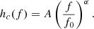
For example, a population of GW-driven circular SMBHBs produces a spectrum with α = −2/3 and amplitude A ≈ 10−15, assuming f0 = 1yr−1. hc(f) is connected to the differential energy content of the signal per logarithmic frequency through the equation:
where H0 is today’s Hubble expansion parameter. We note that hc(f) and Ω(f) provide equivalent parametrizations of the spectrum. The former is more popular in the astrophysics domain, whereas the latter is the preferred choice for early Universe and cosmology.
Given hc(f), the one-sided power spectral density induced by the GW signal in the timing residuals is given by (Lentati et al. 2015):
where γ = 3 − 2α. PTAs search for HD correlated time delays with such a power spectrum in the data, and measure the parameters A and γ. For an observation timespan T, measurements are discretised in frequency bins Δfi = fi + 1 − fi, where fi = i/T. It is then customary to convert S(f) in RMS residual induced in the TOAs in each frequency bin:
The main properties of the GWB signal observed in DR2new and examined in this paper are shown in Fig. 1. The length of the dataset is T = 10.3 years, and excess common correlated power is detected in several frequency bins up to ≈30 nHz (Fig. 1 left panel). Conversely, some bins are unconstrained, which results in a relatively loose determination of the spectral properties of the observed signal. In the literature, hc and S in Eqs. (1) and (3) are usually anchored to the pivotal frequency f0 = 1 yr−1. The data are, however, most informative at the lowest frequencies, while the common power at 1 yr−1 is essentially unconstrained. This naturally leads to a strong degeneracy of the A − γ 2D posterior, as shown for example in Fig. 1 of Paper III. Therefore, unless otherwise stated, we change the reference frequency to f0 = 10 yr−1, where the data are actually constraining, which results in a weaker dependence of A upon γ, as shown in the right panel of Fig. 1.
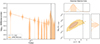 |
Fig. 1. Properties of the common correlated signal detected in DR2new. Left panel: free spectrum of the RMS induced by the excess correlated signal in each frequency resolution bin (with width defined by the inverse of the data span, Δf = T−1). The straight line is the best power-law fit to the data. Right panel: joint posterior distribution in the A − γ plane. Note that we normalise A to a pivotal frequency f0 = 10 yr−1. |
In the following three sections, we discuss three possible contributions to the signal, probing completely different epochs and scales of our Universe, and the implications for the associated physical processes. Namely, the cosmic population of SMBHBs (at redshifts z ≲ 1), the early Universe (z > 1000), and DM (within our Galaxy).
3. Implications I: supermassive black hole binaries
A cosmic population of SMBHBs is the primary astrophysical candidate to produce a signal in the nanohertz band detectable by PTAs. If we define d5N/(dzdm1dqdedtr) as the cosmic merger rate of SMBHBs as a function of redshift, primary black hole mass, mass ratio, and eccentricity, the general form of the generated GWB as a function of observed frequency f can be written as (Sesana 2013a)
![$$ \begin{aligned}&h_c^2(f) = \int _0^{\infty }\mathrm{d}z \int _0^{\infty }\mathrm{d}m_1\int _0^{1}\mathrm{d}q \frac{\mathrm{d}^5N}{\mathrm{d}z\mathrm{d}m_1\mathrm{d}q\mathrm{d}e\mathrm{d}t_r}\frac{\mathrm{d}t_r}{\mathrm{d}\mathrm{ln}f_{\mathrm{K},r}}\nonumber \\&\qquad \quad \times h^2(f_{\mathrm{K},r})\sum _{n=1}^{\infty }\frac{g[n,e(f_{\mathrm{K},r})]}{(n/2)^2}\bigg |_{f_{K,r}=f(1+z)/n}. \end{aligned} $$](/articles/aa/full_html/2024/05/aa47433-23/aa47433-23-eq5.gif)
Here, dtr/dlnfK, r is the time spent by the shrinking binary within a given logarithmic orbital frequency bin, which converts the merger rate into the distribution of rest-frame orbital frequencies of the emitting population. This quantity depends on the physical processes driving the evolution of the SMBHBs including, besides GW emission, interaction with the stellar and gaseous environment surrounding them. As such, it is generally a function of the binary parameters m1, q, e, and extra parameters describing the environment, such as the stellar density in the nucleus of the galaxy host (for more details, see Sesana 2013a). The second line of Eq. (5) is the strain amplitude produced by each individual eccentric SMBHB binary, cast as the sum of harmonics fulfilling the condition fK, r = f(1 + z)/n. In that expression, h(fK, r) is the strain of the equivalent circular binary emitted at twice the orbital frequency of the system, as given in Eqs. (4)–(7) of Rosado et al. (2015), and g(n, e) is a combination of Bessel functions (see, e.g. Bonetti & Sesana 2020, for details). For a distribution of circular, GW-driven binaries, the only relevant mass parameter is the chirp mass ℳ = (m1m2)3/5(m1 + m2)1/5, and Eq. (5) takes the familiar form (Sesana et al. 2008)
This can be recast in terms of the comoving number density of merging binaries d2n/(dzdℳ) (Phinney 2001)

which highlights that, in this case, the expected spectrum follows a power law hc ∝ f−2/3, and the only free parameter is its overall amplitude. The latter is set by the function d2n/(dzdℳ), which contains all the astrophysical knowledge of the cosmic population of merging SMBHBs, and is determined by the cosmological hierarchical assembly of galaxies and their central SMBHs. Conversely, in the most general case described by Eq. (5) there is also information in the spectral shape of the signal, since coupling with the environment as well as eccentricity affect the function dtr/dlnfK, r, suppressing signal at the lowest frequencies. Moreover, eccentricity distributes the GW power at several higher harmonics of the orbital frequency, slightly modifying the power-law behaviour at high frequencies. In general, the GWB cannot be cast in term of a simple analytical form, although a broken power-law is a sufficient approximation for most situations (see, e.g. Ravi et al. 2014; Sesana 2015; Kelley et al. 2017; Chen et al. 2017b).
The literature investigating the GWB produced by a population of SMBHBs is vast, dating back to the mid-nineties and early 2000s (Rajagopal & Romani 1995; Jaffe & Backer 2003; Wyithe & Loeb 2003; Sesana et al. 2004), and predictions have been made by employing different models and techniques. Models can be broadly classified into two categories: self-consistent theoretical models for SMBH evolution within their galaxies (Sesana et al. 2008, 2009; Ravi et al. 2012; Kulier et al. 2015; Kelley et al. 2017; Bonetti et al. 2018; Siwek et al. 2020; Izquierdo-Villalba et al. 2022), and empirical models based on observed properties of galaxy pairs coupled to SMBH-host galaxy relations (Sesana 2013b; Rosado et al. 2015; Ravi et al. 2015; Simon 2023), or on the evolution of the SMBH mass function inferred from observations (McWilliams et al. 2014). Note that we group both semianalytic models (SAMs) and large cosmological simulations in the first class. The main difference between these two classes is that self-consistent models are constructed to reproduce a large array of observations related to galaxies and the SMBH they host, such as the redshift-dependent galaxy mass function, quasar luminosity function, and so on. Conversely, empirical models are, by construction, consistent with the observations upon which they are based, but are usually not tested against independent constraints. As a consequence, they can generally produce a wider distribution of GWB amplitudes, but consistency with other observations is not necessarily guaranteed.
In this section, we investigate the implications of the signal observed in the DR2new dataset for representative models of the two classes. In Sect. 3.1, we perform a semi-quantitative comparison between the measured signal and predictions of an extended version of the Rosado et al. (2015) models (hereinafter RSG15) including binary eccentricity and environmental coupling. In Sect. 3.2, we exploit the framework developed in Middleton et al. (2016), Chen et al. (2017a, 2019) to draw inference on SMBHB astrophysics from the data, either by assuming astrophysical priors from independent observations, or by using a completely generic model for the SMBHB mass function with minimal assumptions. In Sect. 3.3, we demonstrate how the measured signal can inform galaxy and SMBH formation models by examining its constraining power on two state-of-the-art SAMs, namely L-galaxies (Henriques et al. 2015) and the model developed by Barausse and collaborators (Barausse 2012; Bonetti et al. 2018; Barausse et al. 2020). We discuss caveats and future directions of improvement in Sect. 3.4.
3.1. Qualitative analysis of empirical SMBHB population models
To carry out a semi-quantitative comparison between observations and empirical models, we use an extended set of SMBHB populations based on the work of Sesana (2013b; S13 hereinafter) and RSG15.
3.1.1. Description of the models
As described in S13, the models are constructed around the number density of merging SMBHs per unit primary mass, mass ratio, and redshift, d3n/(dm1dqdz) obtained by combining different observations of the galaxy mass function and pair fraction, estimated galaxy pair merger timescales, SMBH-host galaxy relations, and prescription for SMBH accretion during mergers (see Sect. 2 of S13 for full details). Given the large uncertainties in all of the ingredients, the models predict a broad distribution of expected GW amplitudes, as shown in Fig. 2.
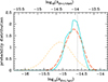 |
Fig. 2. GWB amplitude distributions predicted by the RSG15 models. The thin-dashed yellow line is for the full set of models in RSG15, whereas the thick-dashed orange line is for the subset considered here. The solid blue line is the distribution predicted by the 108 down-selected sample used in the analysis. The vertical line marks the median value of A at f0 = 1 yr−1 reported in Paper III when fixing γ = 13/3 in the search. Note that the lower x-axis scale is for A at f0 = 1 yr−1, whereas the upper x-axis is for A at f0 = 10 yr−1 (the normalization used in this paper). Since α = −2/3 for circular GW-driven binaries, there is a shift of 0.666 dex between the two. |
Guided by the relatively large amplitude of the detected signal and by theoretical and observational advancements in the last decade, we select a sub-sample of those models, as we now justify. First, hydrodynamical simulations of merging galaxies at different scales as well as deep X-ray observations of merging galaxies support accretion activation onto the individual SMBHs prior to merger (e.g. Capelo et al. 2017; Koss et al. 2018). Moreover, hydrodynamical simulations of sub-pc scale binaries, have found most of the accretion to occur on the secondary (i.e. less massive) SMBH (Farris et al. 2014). We therefore restrict the analysis to models where SMBHs accrete prior to the merger, either with an equal Eddington ratio or with preferential accretion onto the secondary3. Second, observations of overmassive black holes in the centre of large ellipticals (McConnell et al. 2011) has led to an upward revision of the SMBH-galaxy relations. Contrary to S13 and RSG15, here we consider only those revised realations, namely the ones reported by Kormendy & Ho (2013), McConnell & Ma (2013), Graham & Scott (2013). Finally, given the large number of models, to save computing power, we perform an ad hoc down-selection of 108 models that preserves the overall distribution of the expected GWB amplitudes, as shown in Fig. 2.
As opposed to RSG15, we go beyond the circular-GW driven binary approximation and consider the self-consistent evolution of SMBHBs within their stellar environment4. This is done by employing the hardening models of Sesana (2010) that self-consistently evolve the SMBHB semimajor axis and eccentricity under the combined effect of stellar hardening and GW emission, once a given initial eccentricity e0 at binary formation is given. Those evolutionary tracks allow us to evaluate the term dt/dlnfK, r in Eq. (5), and thus to reconstruct from the density distribution of merging binaries, d3n/(dm1dqdz), the numerical distribution of systems emitting at any time in the whole sky as a function of mass, mass ratio, redshift, orbital frequency and eccentricity, d5N/(dm1dqdzdfde). For each model, we consider 10 values of e0 = 0, 0.1, ..., 0.9 and three different normalizations of the stellar density profile, described as ρ = C × ρ0(r/r0)−1.5, with C = 0.1, 1, 10 (details in Sesana 2010).
In total, we explore 108 × 10 × 3 = 3240 models, spanning different eccentricities and densities of the stellar environment. For each model, we draw 100 Monte Carlo samplings of the distribution of the emitting binaries, we discretise the frequency domain in bins of Δf = 10.3 yr−1, and add the signals of binaries falling in the same bin in quadrature. This leads to the binned characteristic strain spectrum hc(f) that we then convert in S(f) and RMS residuals using Eqs. (3) and (4). The full procedure is described in Amaro-Seoane et al. (2010), Bonetti & Sesana (2020). In this way, we generate a grand total of 324k Monte Carlo realizations of the predicted GW spectrum in the PTA band.
3.1.2. Comparison with the observed signal
The binned spectrum shown in Fig. 3 contrasts expectations from the 324k models (green) to the measured correlated signal in DR2new (orange). The two sets of violin plots are in good agreement in the few lowest frequency bins, where measurements are the most constraining. Note that the model prediction distributions are highly non-Gaussian and asymmetric, with long tails extending upwards. This is due to the fact that sparse very massive/nearby binaries can sometimes produce exceptionally loud signals, as illustrated by the 100 individual GWBs overplotted to the violins. In fact, this might explain the extra power measured in the 4th and, most strikingly, in the 9th lowest bins compared to the bulk of the model predictions. We caution that the 9th bin is close to the 1 yr−1 mark, where PTAs are blind due to fitting for the Earth orbital motion, and leakage from imperfect fitting might affect that measurement. In any case, if this extra power is indeed due to GWs, it can be easily accommodated by theoretical models, as demonstrated by the realization highlighted by the tick grey line.
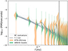 |
Fig. 3. Free spectrum violin plot comparing measured (orange) and expected (green) signals. Overlaid to the violins are the 100 Monte Carlo realizations of one specific model; among those, the thick one represents an example of a SMBHB signal consistent with the excess power measured in the data at all frequencies. |
Our Monte Carlo approach to generate the SMBHB population and its associated GW signal also allows us to investigate the occurrence of CGWs in the data, for which evidence in DR2new is found to be inconclusive (EPTA Collaboration & InPTA Collaboration 2023c). Since the search performed in that paper was limited to circular binaries, we only carry out this analysis for the 32.4k models with e0 = 05. A full assessment of the detectability of CGWs requires the evaluation of the detection probability of each individual binary for a given false alarm rate, as detailed in RSG15. For the sake of simplicity, and given the qualitative nature of this analysis, we just compute the signal-to-noise ratio (S/N) of each individual binary according to Eq. (46) of RSG15 (thus also restricting to the Earth term only). When computing the S/N of a source, we model each pulsar noise by using the maximum likelihood values of the single pulsar noise analysis presented in EPTA Collaboration & InPTA Collaboration (2023a), and add the GWB produced by all of the other binaries to the noise spectral density. We arbitrarily set the detectability threshold at S/N = 3 in the following.
Results are shown in Fig. 4, which compares the power distribution of resolvable CGWs to the binned spectra of the overall predicted GW signal and of the DR2new measurements. In line with RSG15, the probability of detecting a CGW is maximum at the lowest frequency, rapidly decaying to less than 0.01 past the 6th bin. Although this seems to suggests that the feature observed at the 9th frequency bin is unlikely to be due to a CGW, it should be noticed that we considered here a threshold of S/N = 3. The overall GW signal in our data has a total S/N ≈ 3.5 − 4 (EPTA Collaboration & InPTA Collaboration 2023b), mostly accumulated at the lowest frequency bins. It might still be the case that the feature at the 9th bin is due to an unresolved CGW with S/N < 3, which would be a more common occurrence in the data. Note that the average S/N of CGWs slightly increases at higher frequencies, which is primarily due to the frequency dependence of the CGW characteristic strain, hc ∝ f7/6. If pi is the probability of having a CGW of S/N > 3 in the ith bin, we can compute the probability of detecting at least one CGW with S/N > 3 in DR2new according to these models as p = 1 − ∏(1 − pi), which gives p = 0.49. It is therefore quite possible that the observed signal is dominated by few bright sources, which might be resolvable in the future with more sensitive datasets. Thus far, searches for CGWs on the current dataset yielded inconclusive evidence (EPTA Collaboration & InPTA Collaboration 2023c). This probability is obviously S/N threshold dependent. For example, by increasing this threshold to S/N > 5, we get p = 0.13. This is comparable to the 6% chance found by Bécsy et al. (2022). and the slightly larger probability in our models is likely due to the louder overall amplitudes of the signals considered here. We stress, however, that these findings apply to models where binaries remain essentially circular. The number of resolvable CGWs, tends, in fact, to slightly decrease when the eccentricity increases (Truant et al. in prep.).
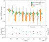 |
Fig. 4. Expected properties of CGWs as a function of frequency. Top panel: free spectrum violin plot comparing the measured signal (orange) to the power distribution of CGWs (green). Empty violins show the full GWB produced by the models for comparison. Bottom panel: the probability of detecting a CGW with S/N > 3 as a function of frequency (green circles, left y-axis scale). The average S/N of CGWs is also shown as red crosses (right y-axis scale). |
Finally, we once again propose the comparison first shown by Middleton et al. (2021), who contrasted the measured 2D A − γ posterior to model expectations. For the latter, we just fit the 9 lowest frequency bins of the GWB spectrum of each Monte Carlo realization of the Universe with a straight line in the logA − logf plane. As described in Sect. 2, we normalise the measurement to f0 = 10 yr−1, where our data are informative, which alleviates the A − γ degeneracy in the posterior. Results are shown in Fig. 5. Although the measured spectrum tends to be shallower than the theoretical one (see also Sect. 3.4), the contours overlap at 2σ and the marginalised amplitudes are broadly consistent.
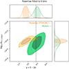 |
Fig. 5. A − γ distribution of the measured signal (orange) compared to model predictions (green). 1σ and 2σ contours are displayed. Shown are also the marginalised A (left) and γ (right) distributions, with their 1σ credible intervals highlighted as shaded areas. |
3.2. Inference on the SMBHB population.
After checking the general compatibility of the observed signal with expectations from empirical SMBHB population models, we take a more quantitative approach and exploit Bayesian inference to constrain the properties of SMBHBs from the data. We repeat the analysis carried out by Middleton et al. (2021) on the common signal detected in the NANOGrav 12.5 year dataset (Arzoumanian et al. 2020), exploiting the framework laid out in Middleton et al. (2016), Chen et al. (2017a, 2019). The SMBHB population of a given model M is described by a set of parameters {θ}, we then use Bayesian inference to find the posterior distribution p(θ|d, M) for the parameters θ of model M given the observation data d:
Here, p(θ|M) is the prior distribution on the model parameters, p(d|θ, M) is the likelihood of model M with parameters θ of producing the data, and p(d|M) is the evidence. For each set of θ, the likelihood is computed by comparing the signal amplitude produced by M at frequencies fi = i/(10.3yr),i = 1, ..., 9, to the posterior distribution of the correlated signal measured in DR2new at the same frequencies. We treat each bin as independent, therefore the likelihood takes the form
where p(A, fi) is the probability density of the amplitude A of the correlated signal measured in the ith bin, and it is evaluated at the value AM predicted by the model. We estimate the likelihood in each bin using a KDE estimate of the DR2new posteriors, similar to the method used in Moore & Vecchio (2021).
Note that the models we use are deterministic in the sense that they have a 1:1 correspondence between θ and the predicted hc(f). In reality, given θ, the ensemble of SMBHBs generating the signal is statistically drawn from the deterministic distribution function, which results in a significant scatter of hc(f), as demonstrated by the individual spectra shown in Fig. 3. We caution that this variance is not captured by these models, and its inclusion in the Bayesian inference pipeline is the subject of ongoing work.
As in Middleton et al. (2021), we use two models to describe the SMBHB population, which are described in turn below.
3.2.1. Agnostic SMBHB population model
The agnostic model, developed in Middleton et al. (2016), makes minimal assumptions about the underlying population of SMBHBs. Binaries are assumed to be circular, GW-driven and the characteristic strain is computed according to Eq. (7) where the source distribution is described by a Schechter function (Schechter 1976) in z and ℳ,
![$$ \begin{aligned} \frac{\mathrm{d}^{2}n}{\mathrm{d}z\mathrm{d}\log _{10}{\mathcal{M} }} = {\dot{n}}_{\rm 0}\left[\left(\frac{{\mathcal{M} }}{10^7{{M}_{\odot }}}\right)^{-\alpha _{{\mathcal{M} }}} e^{-{\mathcal{M} }/{\mathcal{M} }_{\star }}\right] \left[ \left( 1+z \right)^{\beta _{\rm z}} e^{-z/z_{\rm 0}}\right] \frac{\mathrm{d}t_{\rm R}}{\mathrm{d}z}\,, \end{aligned} $$](/articles/aa/full_html/2024/05/aa47433-23/aa47433-23-eq10.gif)
where tR is the time in the source frame and we assume cosmological parameters from Planck18 (Planck Collaboration VI 2020). The five model parameters are θ = {ṅ0,αℳ,ℳ⋆,βz,z0}, where ṅ0 is the merger rate per unit rest-frame time, co-moving volume, and logarithmic ℳ interval, and the parameter pairs {αM, ℳ⋆} and {βz, z0} control the shape of the ℳ and z distributions, respectively. The integration limits in ℳ and z are 106 ≤ ℳ/M⊙ ≤ 1011 and 0 ≤ z ≤ 5, respectively. The prior ranges of the five model parameters are identical to those used in Middleton et al. (2021).
3.2.2. Astrophysically-informed SMBHB population model
The astrophysically-informed model was developed in Chen et al. (2019). This model captures the interaction between the SMBHBs and their environment and allows for eccentric orbits, both of which lead to a characteristic amplitude that does not follow a simple single power law, as in Eq. (5). The model has 18 parameters, 16 of which describe astrophysical observables linking the number of SMBHB mergers to the number of galaxy mergers. The galaxy stellar mass function is modelled as a redshift-dependent Schechter function defined by five parameters: {Φ0, ΦI, M0, α0, αI}. Both the galaxy pair fraction and merger timescales have power law dependencies on the primary galaxy stellar mass M, mass ratio q and redshift function (1 + z) and each of them is defined by a set of four parameters: {f0, αf, βf, γf} for the pair fraction, and {τ0, ατ, βτ, γτ} for the merger timescale:
Galaxy pairs are then populated with SMBHs of mass m following a standard black hole to stellar bulge mass relation of the form
where 𝒩{x,y} is a log normal distribution with mean value x and standard deviation y, which adds three further parameters, {M*, α*, ϵ}, to the model. The final two parameters describe the eccentricity at SMBHB pairing {e0} and the density of the stellar environment {ζ0}. For the 18 parameters listed above, in the analysis presented here, we use the extended prior intervals listed in Table I of Chen et al. (2019).
3.2.3. Results of the inference
The main results of the inference are shown in Figs. 6–8. Figure 6 shows the marginalised posterior distribution for the normalization of the merger rate density ṅ0 from the agnostic model compared to an equivalent parameter derived from the astrophysically-informed model. The constraint on the amplitude of the signal imposes an informative constraint on the normalization of the SMBHB merger density. Using nine frequency bins, the median and central 90% credible regions for log10ṅ0/[Mpc3 Gyr] are  and
and  for the agnostic and astrophysically-informed models, respectively. The measurement essentially constrains the amplitude of the signal, which imposes an informative constraint on ṅ0. The astrophysically-informed model clearly shows that the signal favours an ṅ0 at the upper edge of the astrophysical prior. All other parameters of the agnostic model are unconstrained and the posterior is very similar to the prior (see Appendix A for full posterior distributions for both models).
 |
Fig. 6. Marginalised posterior distributions for ṅ0 using two SMBHB population models. The orange and green open histograms show marginalised posteriors for the agnostic and astrophysically-informed models, respectively. The filled-green histogram shows the prior for the astrophysically-informed model (the prior for the agnostic model is uniform in the range [ − 20, 3]). The vertical dotted lines show the 5th and 95th percentiles of the posteriors. |
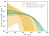 |
Fig. 7. Posterior distribution of the chirp mass function of merging SMBHBs for both the agnostic (orange) and astrophysically informed (green) models. For both models, shaded areas are the central 50% and 90% credible regions and the dashed lines show the medias. The black-dotted lines show the central 99% region for the astrophysical prior. |
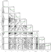 |
Fig. 8. Posterior distribution of selected parameters for the astrophysically-informed model using nine frequency bins of the free spectrum for the inference. Parameters are described in Sect. 3.2.2. |
Figure 7 displays the posterior on the SMBHB chirp mass function for the two models integrated over the redshift range 0 < z < 1.5. Although the agnostic model results in a loosely constrained mass function, the measured PTA signal alone places interesting lower limits on the SMBHB binary merger rate in the Universe. For example, we can say at 95% confidence that for each comoving Gpc3, there have been at least 104 SMBHB mergers with ℳ ≈ 107 M⊙ since cosmic noon. When astrophysical priors weights in, the mass function of merging SMBHBs is well constrained by the PTA signal and, as expected from Fig. 6, it lies in the upper range of the astrophysically informed prior. Within this model, the DR2new measured signal implies there have been about 106 SMBHB mergers for each comoving Gpc3, with ℳ ≈ 109 M⊙ since z = 1.5. This points towards a very active merger history of massive galaxies and a very efficient dynamical evolution of the SMBHBs forming in the merger process.
For the astrophysically informed model, DR2new also provides interesting information on several model parameters. This is because the astrophysical prior considerably narrows down the range of signal amplitudes allowed by the model, and the measured signal pushes towards the upper bound of this range. This results in informative constraints on several key parameters, related in particular to the SMBHB merger timescale and the SMBH-bulge mass relation. As shown in Fig. 8, the SMBH merger timescale τ0 following galaxy pairing must be shorter than ≈1 Gyr (90% confidence), with the data mildly favouring shorter merger times for massive galaxies at low redshifts (i.e. ατ, βτ < 0). Moreover, the data favour a high normalization of the SMBH-bulge mass relation 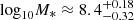 , compared to a much wider prior range extending all the way down to log10M* = 7.8. This is in line with the qualitative analysis of Sect. 3.1, which showed that the signal is consistent with recent, upward-revised, SMBH-galaxy relations. There is also a slight preference for a high normalization of the pair fraction f0 with a positive z dependence, βf > 1. Despite the low γ value favoured by the data, indicative of a flatter spectrum compared to the canonical value predicted by circular GW-driven binaries, SMBHB dynamics is largely unconstrained, perhaps with a marginal preference for eccentric binaries evolving in dense environments (e0 and ζ0 posteriors slightly rising towards the right bound of the prior).
Altogether, these results point towards efficient orbital decay of SMBHBs in the aftermath of galaxy mergers, providing direct evidence that the ‘final parsec problem’ is solved in nature and that compact sub-parsec SMBHBs must be common in the centre of massive galaxies.
3.3. Implications for SAMs
We now explore the implication of this signal for the joint modelling of the galaxy and SMBH formation and evolution by taking a close look at two state-of-the-art SAMs: the model constructed by Barausse and collaborators (Barausse 2012; Sesana et al. 2014; Antonini et al. 2015; Klein et al. 2016; Bonetti et al. 2018; Barausse et al. 2020) and L-Galaxies (Henriques et al. 2015; Izquierdo-Villalba et al. 2022). In this preliminary study, we do not model the dynamical evolution of the binaries and we assume them to be circular and GW driven, thus resulting in a characteristic strain spectrum with α = −2/3.
3.3.1. SAMs and SMBHB delays
In Fig. 9, we show this comparison for the model of Barausse (2012) in its original version (B12) and its subsequent evolutions, which were used to produce the results of Klein et al. (2016, K+16), Bonetti et al. (2018, B+18) and Barausse et al. (2020, B+20). Besides the specific SAM implementation and (astro)physics, these models mainly differ for the physical prescriptions describing the delays between galaxy and MBH mergers, with (i) models “LS-nod (B12)”, “HS-nod (B12)”, “Q3-nod (K+16)”, “LS-nod-noSN (B+20)”, “HS-nod-noSN (B+20)” and “HS-nod-SN-high-accr (B+20)” assuming no such delays (except for the delays between the mergers of the halos and those of the corresponding baryonic components)6; (ii) models “popIII-d (K+16)”, “Q3-d (K+16)”, “LS-d (B+18)”, “HS-d (B+18)” additionally introducing the effect of stellar hardening, triple MBH interactions and gas-driven migration; and (iii) models “LS-noSN-d (B+20)”, “LS-SN-d (B+20)”, “HS-noSN-d (B+20)” and “HS-SN-d (B+20)” accounting for even longer delays (including large contributions from SMBHB separations of hundreds of pc). Note that the labels “SN” (and “noSN”) refer respectively to a putative effect of SN feedback on black hole accretion (and the absence thereof), while “LS”/“popIII” and “HS”/“Q3” denote respectively light and heavy high-redshift seeds for the black hole population.
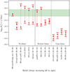 |
Fig. 9. Predictions for the GWB characteristic strain amplitude at f = 1/10 yr from a range of SAMs published in the literature, assuming quasicircular orbits and no environmental interactions (i.e. γ = 13/3), but different physical prescriptions for the delays (increasing from left to right) between galaxy mergers and black hole mergers. The “no delays”, “medium delays” and “long delays” models correspond respectively to the classes of models (i), (ii) and (iii) defined in the text. The ranges account for the finite resolution of the models. The shaded area is the DR2new 95% confidence bound. More details about the models are provided in the text. |
The predictions are computed by summing the gravitational energy spectra of all the SMBHBs in each model’s theoretical population, assuming quasi-circular orbits. As a result, the spectrum has a slope of γ = 13/3 and has no cosmic variance (i.e. we do not account at this stage for the scatter from one realization of the SMBHB population to another). The range shown for each model represents the uncertainty due to the correction for the finite resolution of the SAM’s merger tree. In more detail, the lower end of the range represents a model’s prediction at the finite resolution, while the upper end is the extrapolation – performed as described in Fig. 4 of Klein et al. (2016) – to infinite resolution. The lower arrow (pointing up) should therefore be interpreted as a lower limit, while the upper arrow (pointing down) should be understood as an upper bound (due to the uncertainty of the extrapolation procedure). The extrapolation has not been performed for the model HS-nod-SN-high-accr (B+20), for which we report only the (more robust) prediction at finite resolution. The latter already agrees with the measured amplitude, as a result of a higher accretion rate (by a factor ∼4) for SMBHs.
For two of the models in better qualitative agreement with the data (i.e. “HS-nod-SN-high-accr (B+20)” and “HS-nod-noSN (B+20)”), we compare the predicted signal with the measured DR2new free spectrum in Fig. 10. Unlike in the case of Fig. 9, these predictions were obtained for multiple specific realizations of the SMBHB population, following Sesana et al. (2008) 7. The probability distribution function plotted in each bin represents the scatter of these multiple realizations, and should therefore be interpreted as a “cosmic variance”. Similarly, in Fig. 11 we show the theoretical forecasts for A(f = 1/10 yr) from a subset of the models presented above (namely those in qualitative agreement with the data in Fig. 9). These forecasts are obtained by fitting the model predictions (from multiple realizations of the SMBHB population) in the first 9 frequency bins with a power law with γ = 13/3. The error bars represent the 95% confidence regions (accounting for the scatter due to cosmic variance), while the shaded area indicates the 95% confidence region of the posterior for A(f = 1/10 yr) (assuming again γ = 13/3).
 |
Fig. 10. Binned spectrum of the predicted GWB amplitude for models “HS-nod-SN-high-accr (B+20)” and “HS-nod-noSN (B+20)”. The distribution of the predictions represents the scatter among different realizations of the SMBHB population (“cosmic variance”). Also shown are power-law fits to the predictions. |
 |
Fig. 11. Predictions for A(f = 1/10 yr) in various SAMs, obtained by fitting the spectrum in the first 9 frequency bins with γ = 13/3 for multiple realizations of the SMBHB population. The error bars represent the 95% confidence interval for the predictions, and account for the scatter due to cosmic variance. For each model (except for the boosted accretion model HS-nod-SN-high-accr (B+20)), the higher prediction is the extrapolation to infinite SAM resolution, while the lower one is the finite-resolution prediction. The shaded area is the 95% confidence interval for the measurement of A(f = 1/10 yr), fixing γ = 13/3. For HS-nod-SN-high-accr (B+20) we only show the result uncorrected for resolution. |
Overall, this qualitative comparison, while somewhat dependent on the details of the SAM implementation, suggests that (i) large delays arising from the dynamics of black hole pairs at large ∼100 pc separations are disfavoured, (ii) SMBHB mergers proceed efficiently after their host galaxies have coalesced. Moreover, these results seem to suggest that (iii) accretion onto SMBHs proceeds efficiently, possibly resulting in a larger local SMBH mass function at high masses.
3.3.2. L-Galaxies
Next, we explore the implications that the EPTA results have for L-Galaxies (Henriques et al. 2015; Izquierdo-Villalba et al. 2022), a sophisticated SAM constructed on the dark matter merger trees extracted from the Millennium simulation suite (Springel et al. 2005; Boylan-Kolchin et al. 2009). On top of the galaxy physics, L-Galaxies features a comprehensive modelling for the assembly of SMBHs, including gas accretion triggered by galactic mergers and disc instabilities and dynamical evolution of SMBHBs within the galaxy merger process. The latter accounts for dynamical friction (DF), stellar and gas hardening and, eventually, GW emission. All of these processes are governed by a set of parameters that are tuned to reproduce a vast array of observations including, among others, the galaxy mass function and morphological distribution, the quasar luminosity function and the SMBH-host galaxy relations.
Izquierdo-Villalba et al. (2022) found that the standard L-Galaxies tuning results in a GWB with log10A = −14.9 at f0 = 1 yr−1, lower than that measured in DR2new. Here we perform a systematic investigation of how the stochastic GWB at nanohertz frequencies depends upon the parameters governing the physics of SMBHs and SMBHBs in the SAM. To this aim, we run L-Galaxies in the following configurations:
-
std: standard configuration (Izquierdo-Villalba et al. 2022);
-
t_DF_x0.1: SMBH dynamical friction (DF) time reduced by a factor of ten;
-
NO_GAS_HARD: only stellar hardening;
-
growthDF_x10: accretion boosted by ten in the DF phase;
-
boostBH1: gas accretion doubled after galaxy mergers and disc instabilities;
-
boostBH2 gas accretion doubled after galaxy mergers and tripled after disc instabilities;
-
boostBH1_growthDF_x10: adding accretion boost in the DF phase to model boostBH1;
-
boostBH2_growthDF_x10: adding accretion boost in the DF phase to model boostBH2.
Results are shown in Fig. 12. Changes to the dynamics of SMBHs appear to have a minor effect on the amplitude of the GWB. While shortening the DF time (t_DF_x0.1) allows more SMBHBs to merge within the Hubble time, the most massive ones, which are responsible for the bulk of the GW signal, already have short DF timescales, and the overall GW signal is only mildly increased. Turning off gas hardening results in longer-lived SMBHBs that tend to merge at lower redshifts, resulting in louder GW signals. The effect is, however, negligible. Conversely, the tuning of gas accretion can significantly change the masses of the SMBHBs, resulting in a larger impact on the GWB. Model growthDF_x10 leaves the general population of SMBHs untouched, only boosting the growth of those in the dynamical friction phase. This alone increases the level of the GWB by a factor ≈1.5 compared to model std. Finally, the models boostBH1 and boostBH2 increase the gas accretion onto the whole population of SMBHs, making the GWB a factor of 2.5 louder with respect to the baseline model. Boosting accretion onto the whole population and in the hardening phase further amplifies the expected GWB, reaching the upper bound of the measured value (models boostBH1_growthDF_x10 and boostBH2_growthDF_x10 in the figure). Although these models can accommodate the GWB signal measured in PTAs, the boosted accretion and subsequently larger SMBH masses can make it harder to reproduce the observed SMBH mass and quasar luminosity functions (Izquierdo-Villalba et al. 2022). Additionally, more work is required to find a model that can reproduce all observational constraints in the light of the PTA GW signal (Izquierdo-Villalba et al. 2024).
 |
Fig. 12. Predictions for the GWB characteristic strain amplitude at f = 10/yr−1 from a range of L-Galaxies semi-analytical model versions, assuming that hc(f) ∝ f−2/3. The error bars are computed taking into account the cosmic variance. To this end, we divided the Millennium box into 125 sub-boxes and we compute the GWB in each one. The standard deviation provided by the 125 GWBs corresponds to the extension of our error bars. |
3.4. Further considerations on the measured spectrum: eccentricity and statistical biases.
The analyses presented so far give strong indications that the signal is compatible with a cosmic population of SMBHBs swiftly coalescing in the aftermath of galaxy mergers. The relatively flat slope of the measured spectrum might be indicative of strong environmental coupling and high eccentricities, although inference from the data is inconclusive in this respect (see Fig. 8).
The eccentricity of SMBHBs is of particular relevance as it might carry important information on the dynamical processes driving binary evolution at sub-pc scales (see e.g. Roedig & Sesana 2012). While gas-driven dynamics is expected to saturate the binary eccentricity at a value e ≈ 0.4 − 0.6 (Roedig et al. 2011; D’Orazio & Duffell 2021), stellar hardening is known to statistically increase eccentricity without any saturation point (Quinlan 1996), potentially leading to extremely eccentric systems (Sesana 2010). A large binary eccentricity has two important implications for the interpretation of the current data: it flattens the low-frequency spectrum and it speeds up the SMBHB merger process, as inferred by the small τ0 derived in Sect. 3.2.
Low-redshift massive galaxies are generally gas-poor, and stellar-driven hardening represents the main mechanism driving the evolution of the binaries comprising the bulk of the PTA GW signal. Modelling the whole dynamical evolution, from the first galaxy encounter to black hole pairing and final coalescence, is theoretically and numerically challenging and has been the subject of many studies (e.g. Preto et al. 2011; Khan et al. 2012, 2016; Nasim et al. 2021; Gualandris et al. 2022). In particular, the binary eccentricity is very sensitive to the initial orbits of the merging galaxies (Gualandris et al. 2022). In ongoing work (Fastidio et al. in prep), we are connecting the sub-pc dynamics of SMBHBs to the large-scale parameters of the galactic encounters extracted from the IllustrisTNG100 simulation (Pillepich et al. 2018). Preliminary results show that mergers of massive galaxies occur preferentially on nearly radial orbits, potentially resulting in highly eccentric binaries. Figure 13 shows the orbital parameters of a SMBHB formed in a high-accuracy N-body simulation of a representative galactic merger with properties taken from a merger tree in IllustrisTNG100. Merger trees are selected to represent likely PTA sources at low redshifts. The galactic merger is followed from early times through the inspiral, pairing and hardening of the SMBHs via a hybrid numerical scheme able to model the evolution self-consistently from kpc to mpc scales (Dehnen 2014). Despite the intrinsic stochasticity of the processes driving binary formation and hardening (Nasim et al. 2020), binaries tend to form with a large eccentricity, which then further grows due to encounters with background stars, as also found by scattering experiments (Sesana 2010). Although more work is needed to determine the distribution of expected binary eccentricities and current EPTA data are not yet strongly informative, this pilot study shows the potential of using these measurements in the near future to constrain the physics of galaxy and SMBH mergers.
 |
Fig. 13. Orbital parameters (distance between the SMBHs, semi-major axis and eccentricity) of a SMBHB formed in a representative N-body simulation of a galactic merger with parameters drawn from progenitors of likely PTA sources in the IllustrisTNG100-1 cosmological simulation. Mergers are selected from the merger trees of the 100 most massive galaxies at z = 0, based on galaxy mass ratio (major mergers with mass ratio 1 : 4 or higher) and redshift (z ≤ 2). The dashed lines indicate the critical separation af and the corresponding eccentricity ef at the time in the evolution marking approximately the end of the SMBH inspiral due to DF and the beginning of the hardening phase. Dots represent a and e computed from the apoastron-periastron separation of the two SMBHs before pairing in a bound binary. |
When drawing conclusions on the physical properties of the sources of the GW signal, it is useful to bear in mind not only that the constraints on the spectrum are relatively loose (see Fig. 1), but also that the measured parameters can be subject to statistical and systematic biases. To address this, we have conducted an extensive campaign of simulations by injecting and recovering different types of signals in synthetic PTAs mimicking the properties of the EPTA DR2new dataset (Valtolina et al. 2024). We generated individual noises for 25 pulsars using the maximum likelihood values of the measured white noise and drew the red noise and dispersion measure parameters from the posterior distribution of the customised noise models (cite.wm2). We simulated TOAs from multi-frequency observations and added a GWB spectrum from an astrophysical population of circular SMBHBs producing a nominal GWB with 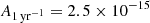 , consistent with the DR2new measurement at γ = 13/3. We performed 100 experiments by changing the specific noise realization and the sampling of the injected SMBHB population. The analysis was carried using the ENTERPRISE software package (Ellis et al. 2020).
Two illustrative examples of injection-recovery mismatch are shown in Fig. 14. The top panel shows one of the GWB recoveries. Although the injection did not present particular features (e.g. loud CGWs), for this specific noise realization, the recovered signal has a shallow slope with a median value of γ = 3.10. Similar cases have been observed when injecting a pure γ = 13/3 power law with the createGWB function of libstempo (Vallisneri 2020). This shows that even with an ideal setup when simultaneously fitting multiple parameters (102 in this case) in a complex problem, the stochastic properties of the noise can easily bias the recovered signal, especially if the S/N is low (S/N ≈ 3.5 for DR2new). Multiple injections with the realistic GWB model and createGWB show systematic biases of recovery of the realistic GWB signal, when modelled with an ideal power law. This is explored in detail in a follow-up work. In the bottom panel of Fig. 14, we show how the presence of some extra high-frequency noise unaccounted for in the MSP noise model can also influence the recovery of the parameters. The setup is the same as in the left panel, but we simulate high-frequency noise mismatch by setting different values of EFAC = 0.8, 1, 1.2 in the recovery. Although the posterior of the signal amplitude is hardly affected, γ can shift significantly depending on whether the high-frequency noise is slightly over- or under-estimated. While these are only two examples, they highlight the complexity of PTA measurements and invite us to be cautious when drawing conclusions that might strongly be influenced by potential biases in the recovered signal.
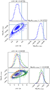 |
Fig. 14. Posterior distributions of the recovered GWB from injections on synthetic data mimicking DR2new. Top panel: statistical offset in an ideal dataset. The square marks the injected value and the blue contours are 1σ and 2σ of the recovered posterior. Bottom panel: effect of high-frequency noise mismodeling on the recovery. The orange, blue and green contours are respectively obtained when EFAC = 0.8, 1, 1.2 are used for the recovery (injected EFAC = 1). |
4. Implications II: physics of the early Universe
Although a GWB generated by an ensemble of the putative SMBHBs is the most plausible source of the observed common-red noise process in pulsar data, more exotic explanations are possible, such as signals originated in the early Universe. The various possible types of cosmological backgrounds of GWs associated with early Universe physics are reviewed in Caprini & Figueroa (2018) and are found to be stochastic. Similarly to the traditional case invoking SMBHBs, the angular spatial correlation for those scenarios follows the HD curve. However, the spectral shapes of the predicted GW spectra are generally different, which can help to disentangle between different types of backgrounds. In this work, we focus on four possible scenarios:
-
An inflationary GWB from the amplification of quantum fluctuations of the gravitational field,
-
A GWB from a network of cosmic string loops,
-
A GWB from vortical (M)HD turbulence at the QCD energy scale,
-
A scalar-induced GWB arising from inflationary scalar perturbations at the 2nd order in perturbation theory.
Given the low significance of the detected signal and the limited number of probed frequency bins due to the short timespan of the data, one cannot currently perform a reliable model selection. Therefore, throughout the section, we consider these scenarios separately and assume that each of them can fully explain the detected signal independently. Analysis invoking more complex models with simultaneous fits for multiple scenarios as well as opportunities to disentangle between those (e.g. Goncharov et al. 2022; Kaiser et al. 2022) will be considered in a number of future works.
4.1. Implications on a stochastic background of primordial (inflationary) gravitational waves
Here we address the GWB possibly generated during inflation (Grishchuk 1975; Rubakov et al. 1982; Starobinskii 1985; Fabbri & Pollock 1983; Abbott & Wise 1984). In the standard inflationary scenario, tensor quantum vacuum fluctuations of the metric are amplified by the accelerated expansion, leading to a GWB as they subsequently re-enter the horizon during the radiation (or matter) era. The cosmic microwave background (CMB) and Big Bang Nucleosynthesis (BBN) provide precise measurements of the radiation energy density, from which one can derive weak upper bounds on the amplitude of such a GWB (see e.g. Caprini & Figueroa 2018, and references therein). Furthermore, tensor metric perturbations lead to CMB temperature anisotropies and polarisation at large angular scales (Sachs & Wolfe 1967; Starobinskii 1985; Kosowsky 1996; Allen & Koranda 1994). Since the anisotropies and polarisation detected so far are due to scalar perturbations, it is possible to constrain the energy density of a GW background by placing an upper limit on the tensor-to-scalar ratio r at CMB scales: recent upper bounds are given e.g. in Tristram et al. (2022), Galloni et al. (2023). Another parameter to consider is the tensor spectral index nT of the tensor perturbations. In the context of slow-roll single-field inflation, these two parameters are linked via the consistency relation r = −8nT. By fixing the consistency relation, Tristram et al. (2022) finds r < 0.032 at 95% CL, while by relaxing it, Planck Collaboration X (2020) finds r < 0.076 and −0.55 < nT < 2.54 at 95% CL.
Within the slow-roll consistency relation, the GWB spectral slope is therefore slightly red-tilted, causing this signal to be out of reach of most current and planned GW detectors such as PTAs, LISA, aLIGO, aVirgo or the Einstein Telescope. On the other hand, it is fair to consider that the spectral slope could vary over the large frequency span ranging from CMB scales to those probed by GW detectors (Lasky et al. 2016). Inflationary scenarios breaking the consistency relation at small scales might therefore produce a detectable GWB, if they lead to a blue-tilted spectrum. In this case, PTAs, LISA and ground-based devices can place upper limits on nT (see e.g. Abbott et al. 2017). It is interesting to investigate which kinds of processes could give rise to a blue-tilted GW background while still obeying CMB constraints at large scales. One possibility is the presence, after inflation, of a stiff component in the Universe, with an equation of state w > 1/3 (Boyle & Buonanno 2008; Giovannini 1998; Boyle & Steinhardt 2008). The enhancement of the tensor spectra can also be produced during inflation thanks to processes such as, for example, (i) particle production during inflation (see e.g. Sorbo 2011a; Barnaby et al. 2012; Cook & Sorbo 2013a; Anber & Sorbo 2012; Bartolo et al. 2016) (ii) enhancement of tensor perturbations for example by spectator fields, or space-dependent inflation (see e.g. Bartolo et al. 2007; Biagetti et al. 2013, 2015; Fujita et al. 2015) (iii) modified gravity theories such as f(R) or Horndeski gravity (Horndeski 1974; Sotiriou & Faraoni 2010) and iv) enhanced scalar perturbations at small scales and/or primordial black holes, which are treated in Sect. 4.4.
4.1.1. Analysis
Similarly to what was done in Lasky et al. (2016), we constrain the key parameters defining the GWB, r and nT, while being agnostic on the underlying process generating the blue-tilted spectrum. If we assume that the common quadrupolar red noise signal present in EPTA data is of inflationary origin, these two parameters can be estimated using the DR2new dataset. Note that the spectral index nT is expected to vary with the frequency scale considered (see e.g. Giarè & Melchiorri 2021; Giarè et al. 2023; Auclair & Ringeval 2022). However, for simplicity, here we consider a constant nT all the way from CMB scales to those corresponding to the (narrow) EPTA frequency band. It is then possible to approximate the fractional characteristic GW energy density using (Lasky et al. 2016; Caprini & Figueroa 2018)
![$$ \begin{aligned}&{\Omega _{\rm GW} (f)=\frac{3}{128}\Omega _{\rm rad}\,r\,\mathcal{P} ^*_{\mathcal{R} }\left( \frac{f}{f_*} \right)^{n_T} \left[\frac{1}{2} \left( \frac{f_{\rm eq}}{f} \right)^{2}+\frac{16}{9}\right]}&\nonumber \\&\quad \,\, \qquad \approx 1.5 \times 10^{-16} \left( \frac{r}{0.032} \right) \left( \frac{f}{f_*} \right)^{n_T}, \end{aligned} $$](/articles/aa/full_html/2024/05/aa47433-23/aa47433-23-eq18.gif)
where the second line is valid in the PTA frequency band, and has been obtained by setting h2Ωrad = 2.47 × 10⁻⁵ with h = 0.67, the amplitude of the scalar spectrum  , and f* ≈ 7.7 × 10⁻¹⁷ Hz related to the CMB pivot scale k* = 0.05/Mpc (Planck Collaboration XVI 2014). feq denotes the frequency entering the horizon at matter-radiation equality.
We then use the nine lowest frequency posteriors of the RMS free spectrum shown in Fig. 1 (see Moore & Vecchio 2021; Lamb et al. 2023; Leclere et al. 2023, for details on the method) to fit the inflationary spectrum of Eq. (14) and obtain posteriors on log10r and nT. Results are reported in Fig. 15. Note that, since γ = 5 − nT, the correlation between the amplitude and spectral index of the signal is compatible with Fig. 5. The 90% credible (symmetric) intervals are  and
and 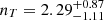 . The obtained value of nT corresponds to a PSD spectral index of γ ≃ 2.7, as in Fig. 1. The excessively small value of r is a consequence of the simplistic parameterisation of Eq. (14), which assumes a constant nT at all scales. The fractional energy density spectrum obtained from the maximum a posteriori parameter values is plotted in Fig. 16.
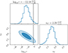 |
Fig. 15. 2D posteriors of the tensor-to-scalar ratio (in log10) and the fractional energy density spectral index nT in the PTA frequency range. The 68% and 95% credible regions are displayed. The black dashed line represents the tensor-to-scalar ratio upper bound found in Tristram et al. (2022) assuming single-field slow-roll inflation. |
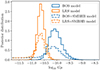 |
Fig. 16. SGWB spectra (in terms of log10h2Ωgw) for four different early Universe SGWB models considered in this paper. BOS/LRS correspond to a cosmic string background with Nc = 2 and Nk = 0 (Γ = 57), and log10Gμ = −10.1/−10.6. The GWB from turbulence is plotted in solid line for λ*ℋ* = 1, Ω* = 0.3, and T* = 140 MeV. The inflationary spectra is shown for log10r = −13.1 and nT = 2.4 (maximum a posteriori value). Power spectrum of the 2nd-order GWB from the scalar curvature perturbations described by the powerlaw model with |

We have so far considered a primordial background to be the only source of GWs in our data. We now recall that the most plausible and loud source of a GW background at these frequencies remains that of a SMBHB background. It is therefore likely that any signature for a cosmological background needs to be considered in parallel with a SMBHB background, or in this case more accurately termed ‘foreground’. Kaiser et al. (2022) have explored the likelihood of detecting a cosmological background in the presence of a SMBHB foreground using simulations, and found that the shallower the slope of the cosmological background (for example γ = 4 as opposed to γ = 5), the harder it is to detect (and the longer it takes, possibly more than 20 years). According to these simulations, this does not bode well for an even shallower slope, similar to the one detected in DR2new with a possible γ < 3.
Here we explore a superposition of these two backgrounds in the DR2new dataset. Considering a two-component GWB for the common red noise model, we place constraints on log10r for given values of nT spanning the range [ − 1, 3]. In this case, our null hypothesis is a GWB from a population of GW-driven circular SMBHBs parameterised only by the PSD amplitude log10A of Eq. (3) (we fix γ = 13/3). We run several analyses with a fixed nT for the inflationary background, sampling over (log10r, log10A). For each of the nT values, we obtain a distribution for log10r and take the 95% quantile as an upper bound. As found in Lasky et al. (2016), nT and the log10r upper bounds are related with good precision by a linear relation:
Our analysis gives a = −0.16 and b = 0.70, which is comparable to the forecast values given in Lasky et al. (2016) (note that they normalise r to 0.11).
4.1.2. Discussion
From the analysis of the DR2new dataset above, we have obtained credible intervals for the tensor-to-scalar ratio r and the spectral index nT. This was performed assuming that reheating is instantaneous, and that inflation is followed directly by the radiation-dominated era, for which the equation of state parameter of the Universe is w = 1/3. Under this assumption, one finds that the best-fit value for the tensor spectral index is nT = 5 − γ ≃ 2.3, which is directly linked to the best-fit PSD spectral index γ ≃ 2.7. This high value of nT is not consistent with slow roll inflation. However, if inflation is followed by a stage in which w ≠ 1/3, the relation between the PSD spectral index γ and the primordial tensor spectral index nT changes to (Arzoumanian et al. 2016; Caprini & Figueroa 2018)
again with γ ≃ 2.7. If a stiff fluid component (w > 1/3) were to dominate the Universe for a finite amount of time after inflation, the last term in Eq. (16) would be bounded between 0 and −2. Hence, nT ≳ 0.3, meaning that even allowing for the presence of a stiff component after inflation, it does not seem possible to explain the common red noise in the context of slow roll inflation (nT ≃ 0) for the best fit value γ ≃ 2.7. However, by broadening the range of possible values to γ ≥ 3, nT ≃ 0 does become compatible with the common red noise.
4.2. Implications on a background of cosmic strings
Cosmic strings are line-like topological defects that may form after a symmetry-breaking phase transition in the early Universe (Kibble 1976; Hindmarsh & Kibble 1995); they are generic predictions of most Grand Unification Theories scenarios (Jeannerot et al. 2003). These 1D objects are characterised by the string tension Gμ (or equivalently their energy per unit length) which is related to the energy scale of the phase transition.
Overall, cosmic strings combine relativistic velocities and large energy densities, making them natural sources of GWs. These GWs may take the form of bursts from cusps, kinks and kink-kink collisions on the loops (Damour & Vilenkin 2001), and have been searched for in the LIGO/Virgo/KAGRA (LVK) detectors (Abbott et al. 2018, 2021). Cusps are points on the string which, in the Nambu-Goto approximation, propagate at the speed of light, and the string doubles back on itself. On the other hand, kinks are discontinuities in the tangent vector of a string and are formed at each intercommutation of strings. The future space-based detector LISA will be sensitive to cosmic string bursts for tensions as low as Gμ ∼ 10−11 (Auclair et al. 2023a). Most notably, in the event that LISA detects GW bursts from cosmic strings, they will likely repeat multiple times a year due to the periodic nature of the cosmic string loops (Auclair et al. 2023b).
The incoherent sum of these GW bursts also produces a stochastic GWB (SGWB), which has been looked for by LVK (Abbott et al. 2018, 2021). LISA is expected to be able to detect a SGWB from cosmic strings with tensions as low as Gμ ∼ 10−17 (Auclair et al. 2020). The strings background has already been looked for in EPTA (Sanidas et al. 2012; Leclere et al. 2023), in NANOGrav (Blasi et al. 2021; Ellis & Lewicki 2021) and PPTA (Bian et al. 2022; Chen et al. 2022). These earlier analyses consistently found a good agreement between the common uncorrelated red signal (CURN) present in the data and a SGWB from cosmic strings with tensions Gμ ∼ 10−10 − 10−11.
4.2.1. Description of the models
Since the SGWB is sourced by sub-horizon cosmic string loops, the central quantity in our analysis is the loop density distribution, n(ℓ, t), where ℓ is the invariant length of the loop (defined by its total energy divided by μ) and t is cosmic time. We focus on the most up-to-date loop distributions, calibrated on large scales with Nambu-Goto simulations (Lorenz et al. 2010; Blanco-Pillado et al. 2014). Loops are formed from the intercommutation of super-Horizon infinite strings, with a maximal size ℓ ≈ 0.1t at time t. (Note that the simulations assume an intercommutation probability of 1, as is the case for field theory strings.) The two models – which we refer to as BOS (Blanco-Pillado et al. 2015) and LRS (Lorenz et al. 2010), after the names of their authors – differ in their treatment of small loops, particularly on scales at which gravitational radiation (not included in numerical simulations) can have important effects. Indeed, compared to the BOS model, the LRS model has an additional population of small loops, which leaves an imprint in the SGWB spectrum (Auclair 2020). The explicit expressions for the two loop distributions are given in Abbott et al. (2018), and both have been considered by the LVK (Abbott et al. 2021) and LISA (Auclair et al. 2020) collaborations. The third observing run of LVK placed constraints on Gμ, based on the non-detection of a SGWB. These are Gμ ≲ 10−8 for BOS and Gμ ≲ 10−15 for LRS. At the frequency of ground-based detectors, the SGWB signal is produced by loops formed during the radiation era. At low PTA frequencies, the SGWB signal is dominated by larger loops, namely those formed at recent times, in transition from the radiation to matter era and also in the matter era (Ringeval & Suyama 2017; Auclair 2020; Leclere et al. 2023).
Other than Gμ, a further parameter appears in n(ℓ, t), namely Γ, which describes the rate at which loops lose energy through gravitational radiation:  . If Γ is large, fewer loops are present in the distribution since loops decay more rapidly. On the other hand, GWs are emitted more intensively: the final effect is a combination of these two, which impacts the SGWB of the BOS and LRS models in subtly different ways (Auclair 2020). The value of Γ depends on the properties of loops, and in particular on how many cusps, kinks, and kink-kink they contain as (Damour & Vilenkin 2001; Siemens et al. 2007; Ringeval & Suyama 2017)
where Nc, k is the number of cusps/kink events per oscillation period of the loop,  the number of kink-kink collisions, and
where  .
.
In this paper, we consider 2 cases. For the first model (i) Nc = 2 and Nk = 0, for which Γ = 57 (Leclere et al. 2023), a value close to that observed in numerical simulations of individual loops (Vachaspati & Vilenkin 1985; Blanco-Pillado & Olum 2017). Therefore, the only free parameter for this model is Gμ. As for the second model (ii), we fix Nc = 1 and allow Nk to vary between 1 and 200 (with a uniform prior) so as to account for theoretical uncertainties on the initial number of kinks at loop creation, and on the efficiency of the gravitational backreaction that should smooth out the loops (see the LVK analysis, Abbott et al. 2021, for a similar approach). Therefore, this is a two-parameter model (Gμ, Nk).
The fractional energy density of the SGWB per logarithmic interval of frequency is given by
![$$ \begin{aligned}&\Omega _{\rm {GW}}(t_0, f) = \frac{16 \pi (G\mu )^2}{3H_0^2} \sum _b \frac{N_b \Gamma ^{(b)}}{\zeta (q_b)}\nonumber \\&\qquad \qquad \times \sum _{n=1}^{+\infty } \int \frac{n^{1-q_b} \mathrm{d} \,{z}}{(1+z)^5 H(z)} \mathbf n \left[\frac{2n}{(1+z)f}, t(z)\right], \end{aligned} $$](/articles/aa/full_html/2024/05/aa47433-23/aa47433-23-eq30.gif)
where H0 is the Hubble constant, H(z) is the Hubble parameter for which we assume standard ΛCDM cosmology with the Planck-2018 fiducial parameters (Planck Collaboration VI 2020), and t0 is the cosmic time today. The sum is over the cusp, kink and kink-kink contributions (labelled with the index b) for which qb = 4/3, 5/3 and 2 respectively.
4.2.2. Analysis results
Our analysis follows the one presented in Leclere et al. (2023), which was based on six pulsars with the best timing precision from the EPTA early Data Release 2 (Chen et al. 2021). We now analyse the DR2new dataset with 25 pulsars, using the (computationally heavy) hierarchical likelihood data analysis method described in Paper III. We sample the SGWB parameters (Gμ) or (Gμ, Nk) as well as the individual pulsar noise parameters.
Solid lines in Fig. 17 show the posterior distribution on log10(Gμ) in case (i), for which Nk = 0 and Γ = 57. The string tension 90% credible (symmetric) interval is  (resp.
  ) for the BOS (resp. LRS) model. The corresponding SGWB spectra are shown in Fig. 16 where, for each model, we set Gμ to their median values. We also consider the two-component SGWB model made of the sum of a background from cosmic strings and one from a population of GW-driven circular SMBHBs characterised by the PSD of Eq. (3). The posteriors of the two background parameters (log10A, log10Gμ) are highly correlated, since both provide a possible explanation for the detected signal. As a result, the posterior on log10Gμ no longer has compact support, but a tail to lower values (see the dashed lines in Fig. 16). We therefore extract the 95-quantile of the string tension posterior to obtain an upper bound of log10Gμ < −9.77 (resp. −10.44) for the BOS (resp. LRS) models.
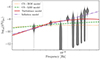 |
Fig. 17. Comparison of the string tension posteriors for the two string models (BOS and LRS) in case (i), Nc = 2 and Nk = 0 (Γ = 57). Solid lines assume only a cosmic string background, dashed lines assume both a population of GW-driven circular SMBHBs and cosmic strings. |
The DR2new dataset exhibits a shallower slope for the PSD of the common red signal than DR2full. While cosmic strings were a good fit to the common red signal of 6 pulsars of DR2full (Leclere et al. 2023), this is no longer true for DR2new. This is because the predicted SGWB PSD is generally steeper than the measured correlated red signal in the data, as can be seen in Fig. 16.
For case (ii), we obtain very similar results to those discussed in Leclere et al. (2023). Namely, we obtain quasi non-informative posteriors for Nk, showing that the data can be equally explained by a population of kinky loops with Nk ≳ 120. In other words, we cannot extract any upper bound on the number of kinks, since this quantity is degenerate with Gμ.
4.3. Implications on background from turbulence around the QCD energy scale
Turbulence can arise in the early Universe in the aftermath of a first-order phase transition (Witten 1984; Kamionkowski et al. 1994), or can be driven by pre-existing primordial magnetic fields (Quashnock et al. 1989; Brandenburg et al. 1996). If the (magneto-)hydrodynamic turbulence were present around the QCD epoch, when the Universe had a temperature of T* ∼ 100 MeV, it would generate a GWB in the PTA band. The characteristic scale of the turbulence, determining the characteristic GW frequency, is in fact related to the (comoving) Hubble radius at that epoch  , where
and g* denotes the number of relativistic degrees of freedom. If a large lepton asymmetry and/or primordial magnetic fields were present in the early Universe, the QCD phase transition might have been of first order (Schwarz & Stuke 2009; Wygas et al. 2018; Middeldorf-Wygas et al. 2022; Vovchenko et al. 2021; Cao 2023). In this case, one would expect additional sources of GWs, from the collision of broken phase bubbles and the subsequent development of sound waves in the primordial fluid (Kosowsky et al. 1992; Kosowsky & Turner 1993; Caprini et al. 2008; Huber & Konstandin 2008; Jinno & Takimoto 2017; Cutting et al. 2018; Hindmarsh et al. 2014, 2015, 2017). This was analysed for PTAs, e.g. in Moore & Vecchio (2021), Arzoumanian et al. (2021), Xue (2021). In what follows, we focus on the GWB generated by decaying (M)HD turbulence.
4.3.1. Description of the model
The presence of bulk velocity and magnetic fields produce anisotropic stresses, which in turn act as a source of GWs (Kamionkowski et al. 1994; Kosowsky et al. 2002; Dolgov et al. 2002; Caprini & Durrer 2006; Gogoberidze et al. 2007; Caprini et al. 2009). This has been recently studied via numerical simulations in Roper Pol et al. (2020a,b, 2022a), Brandenburg et al. (2021). In particular, Roper Pol et al. (2022a) show that the envelope of the GWB produced by decaying MHD turbulence can be estimated analytically, assuming that the anisotropic stresses from the velocity and magnetic fields vary more slowly than the dynamical production of GWs. This was also validated by numerical simulations of purely kinetic turbulence in Auclair et al. (2022). This assumption leads to the following GWB signal:

where Ω* is the ratio of the (M)HD turbulent energy density to the radiation one, and λ∗ℋ∗ is the ratio of the characteristic length scale of the turbulence, λ*, to the comoving Hubble horizon  at the QCD epoch. The parameter 𝒜 ≃ 1.75 × 10⁻³ is the efficiency of GW production8, estimated in Roper Pol et al. (2022a). The function FGW, 0 is the fractional radiation energy density at the epoch of GW generation to its value at the present time. It depends on the temperature scale T* via the number of degrees of freedom g*,
The spectral shape of the GWB signal, Sturb(f), is
![$$ \begin{aligned}&S_{\rm turb} (\lambda _* f) = \, \mathcal{B} \, \bigl (\lambda _* f\bigr )^3 \, p_\Pi (\lambda _* f) \, \nonumber \\&\qquad \qquad \times \left\{ \begin{array}{ll} \ln ^2 \bigl [1 + \mathcal{H}_* \, \delta t_{\rm fin}/(2 \pi ) \bigr ],&\mathrm{\ if \ } f < 1/\delta t_{\rm fin}, \\ \ln ^2 \bigl [1 + \lambda _* \mathcal{H}_*/(2 \pi \lambda _* f) \bigr ],&\mathrm{\ if \ } f \ge 1/\delta t_{\rm fin}, \end{array}\right. \end{aligned} $$](/articles/aa/full_html/2024/05/aa47433-23/aa47433-23-eq38.gif)
where  is a normalising factor, and δtfin denotes the effective duration of the turbulence. The latter can be estimated, from the numerical simulations performed in Roper Pol et al. (2022a), to be
  . The function pΠ(λ*f) in Eq. (23) denotes the spectrum of the anisotropic stresses. For solenoidal fields (e.g. a primordial magnetic field or vortical bulk fluid motion) characterised by a typical correlation scale of the order of the turbulence scale λ*, it is constant for f < 1/λ*. Furthermore, it decays as f−11/3 for f ≳ 1/λ*, if the turbulence is of the Kolmogorov type, as we assume here. Hence, the resulting spectral shape of the GWB in Eq. (21) presents three power laws: f3 at frequencies below the inverse effective duration of the turbulence f < 1/δtfin, f at intermediate frequencies 1/δtfin < f < 1/λ*, and f−8/3 at large frequencies f > 1/λ*.
The GWB produced from vortical (M)HD turbulence is therefore determined by three parameters: the temperature scale T*, the turbulence strength Ω*, and the turbulence characteristic length scale λ∗ℋ∗. By causality, λ∗ℋ∗ is bound to be smaller than one. In general, also Ω* ≲ 1, otherwise turbulence would change the dynamics of the Universe. However, note that the template described above has been validated in principle only for non-relativistic plasma motions, for which Ω∗ ≲ 𝒪(0.1).
4.3.2. Analysis results
As in Sect. 4.1, here we use the fast free spectrum analysis method on DR2new data to constrain the model, considering the nine first Fourier bins of the RMS spectrum of Fig. 1. We use log10-uniform priors for the model parameters, choosing log10(λ*ℋ*)∈[−3, 0], log10Ω* ∈ [ − 2, 0], and log10(T∗/1MeV) ∈ [1,3]. The 2D posteriors obtained are shown in Fig. 18.
 |
Fig. 18. 2D posteriors for the parameters of the background from turbulence around the QCD energy scale obtained using a free spectrum fit on DR2new data. The 68% and 95% credible regions are displayed. |
For values of Ω* below 0.1, the model can only explain the level of correlated noise at the lowest frequency bin if the amplitude of the spectrum is sufficiently high. This can be achieved only if λ*ℋ* is close to 1 and the peak frequency lies within the PTA frequency range, implying T* ∼ 60 MeV. However, at frequencies around the peak, the signal corresponds to a power spectral density for the residuals steeper than γ ∼ 4, which cannot fit the data well. For this reason, values of Ω* ≲ 0.1 are disfavoured.
For larger values of Ω*, the f3 part of the spectrum at frequencies below  can enter the PTA band with a sufficiently high amplitude. Furthermore, the distance between the break at
  and the spectral peak at 1/λ* becomes minimal in the limit Ω* ∼ 1. Both of these characteristics lead to a better fit to the data. This is recovered in the posteriors of Fig. 18, together with the degeneracy between λ*ℋ* and Ω* from the signal amplitude (see Eq. (21)), and the degeneracy between λ*ℋ* and T* from the break at 1/δtfin (note that the dependence of the latter on
  is subdominant).
The model therefore provides a good fit to the data in the limit of large Ω*, close to the upper bound of the prior. The extension of the dataset to longer observation time will be crucial for further constraining this model at low frequencies.
4.4. Implications on the 2nd-order GWB produced by primordial curvature perturbations
It is well-known that scalar, vector and tensor modes of the perturbed metric do not mix at linear order of the Einstein equations (Lifshitz 1946; Baumann 2022). However, scalar curvature perturbations will source propagating tensorial modes (GWs) at the 2nd order in perturbation theory (Tomita 1967; Matarrese et al. 1993, 1998; Noh & Hwang 2004; Carbone & Matarrese 2005; Ananda et al. 2007; Baumann et al. 2007). Such scalar curvature perturbations and associated primordial density fluctuations inevitably exist in the Universe and can be directly constrained by observations of the CMB. The latest Planck data (Planck Collaboration X 2020) suggests that the power spectrum of the curvature perturbations is nearly scale-invariant with the amplitude Aζ ∼ 2 × 10⁻⁹, which implies a marginal energy-density of the generated GWB. Specifically, when projected to the PTA sensitivity band, the fractional contribution of the energy density in the associated GWs becomes Ωgw ∼ 10−24, which is practically non-detectable by current experiments. On the other hand, some models of inflation (see, for example, Di & Gong 2018; Byrnes et al. 2019; Braglia et al. 2020; Yi & Fei 2023) make it possible to produce a sharp increase in the power spectrum of primordial curvature perturbations over many orders of magnitude at small scales.
While the CMB is only capable of directly sampling large cosmological scales with k ∼ 10−3 − 10−1 Mpc−1, small scales stay largely uncovered. PTAs provide a unique opportunity to complement the CMB measurements by indirectly probing the scalar curvature perturbations in a scale range k ∼ 106 − 108 Mpc−1 through the second-order generated GWB, and to place bounds on the steepest possible growth of the power spectrum as well as corresponding models of inflation (Saito & Yokoyama 2009; Bugaev & Klimai 2011; Chen et al. 2020; Dandoy et al. 2023; Zhao & Wang 2023).
In this work, we consider two models of the primordial curvature power spectrum: i) monochromatic and ii) powerlaw. For the former, the primordial spectrum is modelled as:
where Aζ is a dimensionless amplitude and k* is a wavenumber at which the monochromatic power spectrum has a Dirac-delta peak. For the second case:
where ns characterises the slope and k10 yr is a normalizing scale k10 yr = 2π/(10 yr × c), so that  corresponds to dimensionless amplitude at ten years.
In the first scenario, a semi-analytical solution for the induced spectrum of GWB exists and is given by (Kohri & Terada 2018; Espinosa et al. 2018):
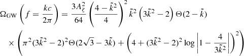
where  and Θ is the Heaviside theta function. In spite of being nonphysical, the δ-function peak approximately describes the maximum of the produced GWB in the inflationary model with the steepest possible k4 growth of a spectral peak in the single-field inflation at small scales (see Fig. 7 in Byrnes et al. 2019).
In the second case of a more general (and more realistic) power-law spectrum, the result can only be obtained numerically (Kohri & Terada 2018):
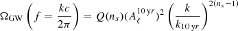
where Q(ns) is the scaling factor which can be evaluated in a range of ns using interpolation points from Table 1 of Kohri & Terada (2018).
After its production, the GWB is damped due to quantum interactions with the particles of the primordial plasma at the radiation-dominated epoch, and redshifted inversely proportionally to the scale factor (as it also occurs to radiation) starting from the epoch of matter-radiation equality (Saikawa & Shirai 2018). The present value of the fractional energy density is then:
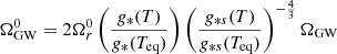
where T is the temperature of the Universe at the moment when structures of a typical size 1/k re-enter the horizon9, Teq is the temperature of the Universe at the epoch of matter-radiation equality, g* and g*s are relativistic degrees of freedom and degrees of freedom in entropy, respectively. The final expression for the auto-power spectral density of the timing residuals is:
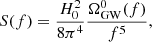
where H0 is the Hubble constant at the present epoch.
The outlined formalism was applied to the DR2new version of the latest EPTA dataset. The number of frequency components which was used for the Fourier representation of the signal was fixed to 9. We have chosen broad uninformative priors for the parameters: uniform in [ − 6, 3] for log10Aζ and  , uniform in [4, 12] for log10(k*/Mpc−1), and uniform in [0.4, 2.6] for ns. Boundaries for the latter are constrained by the limitations of the numerical approximation of the power law model. For this analysis, we assumed that the common red noise process detected in the latest EPTA dataset can be fully explained by the 2nd-order scalar-induced GWs.
Results for monochromatic and power law models are shown in Figs. 19 and 20, respectively. The 2D posterior distribution of the model parameters of the monochromatic model is depicted with orange contours on the right panel of Fig. 19. One may notice that the regions of the highest probability are strongly elongated due to a strong positive correlation between Aζ and k*; these parameters are essentially degenerate. Therefore, DR2new can only provide lower limits on the characteristic scale and amplitude of the monochromatic model: log10(k*, 0.05/Mpc−1) = 7.6 and 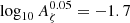 meaning that a whole range of models predicting Dirac-delta power spectrum can equally good describe the signal of DR2new. This behaviour is explained in the left panel of Fig. 19, for which we have simulated GWB signal generated by the monochromatic primordial scalar perturbations, Eq. (26), and attempted to recover a more general power law model of the form S(f)∼f−γ used in Paper III to model an arbitrary common red noise process. After a rapid decrease, the recovered slope stabilises at γ ∼ 3.5 in the limit of large k*, and becomes consistent with both values obtained with DR2new and the theoretically predicted 13/3 for the background from circular, GW-driven SMBHBs. This degeneracy can raise important issues when one tries to disentangle one signal from another. For the power-law case, the 2D posteriors are shown in the left panel of Fig. 20 with the following means and 1-σ uncertainties:
 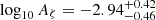 and
and 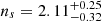 .
.
 |
Fig. 19. Results for the monochromatic curvature perturbations described by Eq. (24). Left panel: recovered slopes γ of a simple power-law model as a function of characteristic scale k* of the injected GWB generated by the monochromatic curvature perturbations. The horizontal lines show the theoretical value of γ from a population of circular, GW-driven SMBHBs (grey) and the one obtained in Paper III (orange). Right panel: 1σ and 2σ contours of the posterior distributions on the amplitude Aζ and characteristic scale of fluctuations k* for DR2new (orange colour). The posterior distribution is overlaid with the current constraints on the primordial power spectrum using Planck data (CMB). The grey colour depicts the 2-σ-confidence intervals. The purple shaded area represents the bounds from spectral distortions (Chluba et al. 2012). For comparison in green we place the prediction of the primordial spectrum of scalar perturbations in the two-field model of inflation described in Braglia et al. (2020) for a range of the model parameters. All three models result in PBH mass functions peaked at ∼35 M⊙ with the brightest line corresponding to the dark matter fraction of PBHs of ∼0.01. |
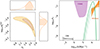 |
Fig. 20. Results for the power-law model of the curvature perturbations described by Eq. (25). Left panel: 1σ and 2σ contours of the posterior distributions on the amplitude Aζ and the slope of the power spectrum ns obtained by the analysis of DR2New. Right panel: 1σ and 2σ contours of the power spectra inferred from the DR2New analysis by picking 1000 random samples from the posteriors overlaid with the current constraints on the primordial power spectrum using the latest Planck data. The grey colour depicts the 2σ-confidence intervals. The green lines and purple shaded areas are the same as in Fig. 19. |
On the right panels of Figs. 19 and 20, we also overplot the inferred primordial power spectrum with the one obtained from the Planck data. The orange areas on the right panel of Fig. 20 are 1σ and 2σ contours of the power-law model described by Eq. (25) reconstructed using 1000 random draws from the posteriors. To explain the observed signatures of the DR2new in terms of the second-order GWB from the primordial scalar perturbations, an excess in the primordial spectrum at low scales should be invoked without violating the CMB inflationary parameters. Such excess has been proposed in many papers, e.g. in the aforementioned works by Ivanov et al. (1994), Germani & Prokopec (2017), Di & Gong (2018), Cai et al. (2018), Biagetti et al. (2018), Byrnes et al. (2019), Motohashi et al. (2020), Braglia et al. (2020), Yi & Fei (2023). Notably, this power excess would lead to a copious production of primordial black holes (PBHs) at the radiation-dominated stage, which is sometimes taken by the authors as the motivation to introduce them as cold dark matter candidates (Carr et al. 2016, and reference therein). The PBH formation from cosmological perturbations has been extensively explored Sasaki et al. (2018). On the radiation-dominated stage, the PBH mass is related to the mass inside the horizon at the time of the perturbation entering,  , where mPl is the Planckian mass, T is the temperature. In terms of the mode comoving wavenumber at the moment of the horizon crossing, k = aH, the part of the horizon mass collapsing into a PBH reads
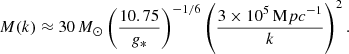
For example, in the two-field inflationary model by Braglia et al. (2020), a peak around k ∼ 2 × 10⁶ Mpc−1 could explain the power Aζ ∼ 10−2 and simultaneously lead to the production of PBHs with masses peaked at ∼35 M⊙ (see also the analysis of the NANOGrav results in Vaskonen & Veermäe 2021). Interestingly, such a peak seems to be observed in the chirp mass distribution of LVK merging binary black holes (Abbott et al. 2023). A more general list of primordial power spectra, as well as a careful retranslation of them to the PBH abundance and their mass function, will be considered in a follow-up paper (Porayko et al., in prep.).
5. Implications III: dark matter
Unlike spatially and temporally-correlated stochastic processes discussed in Sects. 3 and 4, in this section, we explore a possible deterministic contribution to the EPTA signal from ultralight scalar-field dark matter (ULDM). For comparison, the morphology of a putative ULDM signal, predicted by Khmelnitsky & Rubakov (2014), is similar to a CGW from a SMBHB, that is, it is prominent only in one frequency bin. Given that the signal observed with DR2new is mostly apparent in the first two fundamental T−1 frequency bins, it is of interest to consider possible contributions from physical processes with narrowband spectra. Therefore, the analysis presented here complements the CGW interpretation of the signal by EPTA Collaboration & InPTA Collaboration (2023c). Additionally, the ULDM search with DR2full is performed in Smarra et al. (2023).
Dark matter currently constitutes approximately 26% of the energy density of the Universe, as confirmed by, e.g., galactic rotation curves (Rubin et al. 1970, 1980; de Salas et al. 2019), baryonic acoustic oscillations and cosmic microwave background measurements (Bennett et al. 2013; Planck Collaboration VI 2020) as well as galaxy surveys (Escudero et al. 2015). The standard cold dark matter (CDM) picture, whose leading candidates are the weakly interacting massive particles (WIMPs; Arcadi et al. 2018) and the QCD axion (Luzio et al. 2020), successfully grasps the large-scale structure of the Universe. However, it presents some well-known issues, when it comes to explaining observations at scales smaller than 𝒪(kpc). Among these, the cusp-core problem (Flores & Primack 1994; Moore 1994; Karukes et al. 2015) concerns the inconsistency between the observation of a flat density profile in the centre of galaxies and the power-law-like behavior predicated by CDM, while the mismatch between the simulated and observed number of dwarf galaxies in the proximity of our Milky Way is often referred to as the missing satellite problem (Klypin et al. 1999; Moore 1994).
While a thorough understanding of baryonic physics feedback mechanisms (Navarro et al. 1996; Governato et al. 2012; Brooks et al. 2013; Chan et al. 2015; Oñorbe et al. 2015; Read et al. 2016; Morganti 2017) might help to alleviate some of these issues, they can be more easily disposed of assuming that DM is an ultralight (mϕ ∼ 10−22 eV) scalar/pseudoscalar or axion-like field, whose astrophysically large (𝒪(kpc)) de Broglie wavelength suppresses power on small scales. Moreover, ultralight scalars are also generally present in string theory compactifications (Green et al. 1988; Svrcek & Witten 2006; Arvanitaki et al. 2010), which makes them interesting candidates for new physics as well. CMB-based arguments are used to constrain mϕ ≳ 10−24 eV (Hlozek et al. 2015), while Lyman-α bounds push the limit up to mϕ ≳ 10−21 eV, provided that the ultralight particles account for more than 30% of the full dark matter budget (Iršič et al. 2017; Armengaud et al. 2017; Kobayashi et al. 2017; Nori et al. 2018; Rogers & Peiris 2021). A lower limit of mϕ ∼ 10−19 eV is claimed by studies of ultra-faint dwarf (UFD) galaxies (Hayashi et al. 2021; Dalal & Kravtsov 2022), but a wide consensus is yet to be reached. In a seminal work, Khmelnitsky & Rubakov (2014) showed that the travel time of pulsar radio beams is affected by the gravitational potential induced by ULDM particles, making thus PTAs excellent facilities to investigate the existence of ULDM particles. Moreover, they represent complementary probes which do not suffer from the small-scale structure modelling uncertainties that affect non-CMB bounds (Schive et al. 2014; Zhang et al. 2019), as the aforementioned Lyman-α or UFD limits. In the following, we robustly assume that ULDM interacts only gravitationally, therefore giving rise to periodic oscillations in the TOAs of radio pulses as described in Khmelnitsky & Rubakov (2014).
Being non-relativistic and with a very large characteristic occupation number, the ULDM scalar field can be described as a classical wave whose oscillation frequency is twice its mass mϕ (Khmelnitsky & Rubakov 2014). The periodic displacement that ULDM induces on the TOAs of signal from a pulsar P can be written as follows (Porayko et al. 2018):
![$$ \begin{aligned} \delta t(t) = \frac{\Psi _c(\boldsymbol{x})}{2m_\phi } [\hat{\phi }^2_{\rm E}\sin {(2m_\phi + \gamma _{\rm E} )} - \hat{\phi }^2_{\rm P}\sin {(2m_\phi + \gamma _{\rm P} )} ], \end{aligned} $$](/articles/aa/full_html/2024/05/aa47433-23/aa47433-23-eq58.gif)
where
where γP (γE) is a pulsar (Earth) dependent phase and  (
( ) takes into account the stochastic nature of the axion-like field near the pulsar (Earth). The parameters and their priors are summarised in Table 1. Considering a typical value of vϕ ∼ 10−3 for the ULDM velocity, the region in which the scalar field oscillates coherently, i.e. with the same value of
  , is spanned by the coherence length:
Parameters used for the search and their respective priors.
In particular, notice that  and
and  should be taken as:
-
different parameters when the average pulsar-Earth and pulsar-pulsar distance is larger than the coherence length;
-
the same parameter when the average pulsar-Earth and pulsar-pulsar distance is smaller than the coherence length.
Following the procedure in Smarra et al. (2023), we analyze three separate cases, which we refer to as the uncorrelated, the pulsar correlated and the correlated limit. As the average inter-pulsar and Earth-pulsar separation is ∼kpc, the correlated and uncorrelated scenarios stand out as exact limits at the low mass and high mass end of the PTAs band, respectively. Instead, the pulsar correlated limit holds when the coherence length of ULDM is smaller than the Galacto-centric radius probed by rotation curves (inner ∼20 kpc), but larger than the average inter-pulsar and pulsar-Earth distance. More specifically, the correlated regime holds for masses lower than mϕ ∼ 2 × 10⁻²⁴ eV; the pulsar correlated regime for 2 × 10⁻²⁴ eV ≲ mϕ ≲ 5 × 10⁻²³ eV and the uncorrelated limit for mϕ ≳ 5 × 10⁻²³ eV. We defer a more detailed study to future analysis.
Based on the above, we fit the model from Eq. () to the DR2new as in Smarra et al. (2023). As an example, marginalised posterior distributions for Ψc and mϕ are plotted in Fig. 21. All the three limits peak at a ULDM mass mϕ ∼ 10−23 eV with amplitude Ψc ∼ 10−15, which translates into a density ρϕ ≃ 0.6 GeV/cm3 of the scalar field. While this value is higher than the fiducial local DM density ρDM ≈ 0.4 GeV/cm3, it is well within the measurement uncertainties (Bovy & Tremaine 2012; Read 2014; Sivertsson et al. 2018; de Salas 2020).
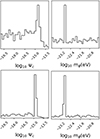 |
Fig. 21. Posterior probabilities for the ULDM amplitude Ψc and mass mϕ, from the correlated (top row) and uncorrelated (bottom row) analysis of the DR2new dataset. The pulsar correlated analysis is not shown, but displays the same features. |
Additionally, we search for a potential ULDM signature alongside the SMBHB gravitational-wave background. Thus, we introduce a new model that contains ULDM contributions alongside a common red signal to account for gravitational wave contributions. We find no ULDM signal under this hypothesis, in agreement with the fact that the data support HD correlation, which naturally favours GWs over ULDM in a joint search. Thus we put 95% upper limit on the amplitude Ψc and the density ρϕ of the scalar field.
Figures 22 and 23 show that the EPTA at current sensitivity is able to constrain the presence of ULDM at the level of the expected DM abundance in the mass range mϕ ∼ [10−24 eV, 10−23.2 eV]. The DR2Full analysis performed in Smarra et al. (2023) pushes these limits down, thus implying that such ULDM candidates cannot constitute the entire DM. We highlight that our bounds extend below the DR2new sampling frequency f = 1/T ≈ 3 × 10⁻⁹ Hz, with T ≈ 10 yr. In fact, while it might naively be thought that the ULDM field needs to complete an oscillation in the timescale τPTA of the PTA experiment to produce a detectable effect, we point out that an ULDM wave with frequency mϕ < 1/τPTA can still be approximated by an expansion in powers of mϕt (Kaplan et al. 2022), though the sensitivity of PTAs will be reduced due to degeneracies with the timing model (Ramani et al. 2020). Relying on the robust CMB bounds mentioned before, we fix the lower end of our search at mϕ = 10−24 eV. Importantly, we remove the  parameter from the search in the correlated limit, as it is fully degenerate with Ψc. In other words, building upon the observation that our Galaxy rotation curve measurements are performed within an ULDM coherence length in the correlated limit, we redefine a new variable,
  , which represents the instance of DM in the Milky Way. Finally, as shown by Fig. 22, we report a bump in upper limits at mϕ ∼ 10−23 eV, which is at around the maximum-a-posteriori boson mass in Fig. 21. This mass further corresponds to the frequency of the CGW analyzed in EPTA Collaboration & InPTA Collaboration (2023c). Looking at the posteriors in this mass range, we also find an additional contribution, on top of the CURN process. A similar bump in upper limits is also present in the DR2Full dataset, as discussed in Smarra et al. (2023). However, the Bayes factor of lnℬ ∼ 0.3 we find in favour of the presence of ULDM signal is still inconclusive. We recommend following up on this bump in future work.
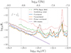 |
Fig. 22. Constraints on Ψc as a function of mϕ using the EPTA DR2new dataset from Paper III. Previous analyses are shown for comparison, cf. Porayko & Postnov (2014), Porayko et al. (2018) for further details. The blue, orange and brown lines represent the 95% Bayesian upper limit on Ψc obtained from the EPTA DR2new dataset with the correlated, uncorrelated and pulsar correlated analysis, respectively. The purple line shows the expected ULDM abundance computed from Eq. (32). |
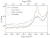 |
Fig. 23. Constraints on the ULDM density ρϕ normalised to the DM background value ρDM = 0.4 GeV/cm3. The blue, orange and brown lines represent the 95% Bayesian upper limit on ρϕ, obtained from the EPTA DR2new dataset with the correlated, uncorrelated and pulsar correlated analysis, respectively. The purple dotted line shows the fiducial local DM density value. |
6. Discussion and outlook
In this paper, we have explored the implications of the common, correlated low-frequency signal observed in the latest data release of the EPTA+InPTA collaboration. Four different datasets were assembled, and the signal was more significant in those including only broadband, high-quality data taken with telescope backends of the new generation. Therefore, we took, as benchmark for our analysis, the signal measured in the DR2new dataset, for which the HD correlation is detected at high significance with a Bayes factor of ≈60 or, equivalently, at a p-value of ≈0.001, indicative of a ≳3σ confidence. The signal can be modelled by a single power law spectrum Sh(f) as in Eq. (3), with best-fit parameters 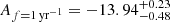 and
and  (Paper III).
We considered several physical processes separately, investigating the implications of the detected signal under the hypothesis that it is generated by that specific process. Our main findings can be summarised as follows.
SMBHBs. The signal is consistent with a cosmic population of merging SMBHBs. Phenomenological models based on galaxy pairs observations can account for the power spectral distribution of the correlated signal. Those models can also be used to predict the chance to detect CGWs in the current data, for which the search has given inconclusive results so far (EPTA Collaboration & InPTA Collaboration 2023c). According to those models, there is roughly a 50% chance to detect a CGW in DR2new at S/N > 3. The relatively high amplitude of the signal can be used to place constraints on key properties of the cosmic SMBHB population. By exploiting the inference framework developed in Middleton et al. (2016), Chen et al. (2019), we can infer that SMBHBs merge in less than 1Gyr following galaxy mergers, and that the SMBH-stellar bulge relation has a normalization log10(M*/M⊙)≈8.4 at a reference stellar mass bulge of 1011 M⊙, in line with recent compiled results (e.g. Kormendy & Ho 2013). Finally, we investigated how the detected signal compares with predictions from state-of-the-art galaxy formation SAMs (Barausse 2012; Izquierdo-Villalba et al. 2022). We found that the high amplitude of the signal imposes non-trivial constraints on galaxy and SMBH evolution models. In particular, boosted SMBH accretion and short SMBHB evolution timescales are needed to match the observed signal, which might lead to difficulties when trying to reproduce independent observables such as the quasar luminosity function. If the SMBHB origin of the observed signal is confirmed, it would be a major breakthrough for observational astrophysics and for our understanding of galaxy formation. This would be the first direct evidence that SMBHBs merge in nature, adding an important observational piece to the puzzle of structure formation and galaxy evolution.
Early Universe. The measured signal would have different implications for each of the physical processes considered in this study. An inflationary origin requires non-standard inflationary scenarios breaking the slow-roll consistency relation, leading to a blue-tilted spectrum. In particular, the measured γ ≈ 2.7 implies nT ≈ 2.3 for a radiation-dominated universe with w = 1/3. A cosmic string origin would allow narrowing down the string tension to values of −11 ≲ log10Gμ ≲ −9.5, depending on the specific distribution of loops in the string network. Conversely, the number of kinks cannot be constrained. A GWB induced by (M)HD turbulence at the QCD energy scale can also potentially explain the common red noise, but requires either high turbulent energy densities, of the same order of the radiation energy density, or a characteristic turbulent scale close to the horizon at the QCD epoch. Finally, the measured signal can be produced by the evolution of scalar perturbations at second order only if an excess of their primordial spectrum is present at large wavenumbers, compared to the level derived from CMB observations at small wave numbers. Notably, such an excess would lead to the production of PBHs which can non-negligibly contribute to the CDM density.
ULDM. Finally, we searched for ULDM signatures in DR2new. The search returned a prominent peak in the posterior distribution of the ULDM particle mass around log10(mϕ/eV)≈ − 23. This corresponds to a field oscillation frequency of log10(f/Hz)≈ − 8.3, which is consistent with the CGW candidate examined in EPTA Collaboration & InPTA Collaboration (2023c). When a joint ULDM+GWB search is performed, however, the peak in the ULDM mass posterior distribution vanishes, as the data strongly prefer the presence of an HD correlation in the common power. We therefore conclude that an ULDM origin of the detected signal is disfavoured, placing a direct constraint on the abundance of ULDM in our Galaxy. The non-detection in DR2new implies that only about 80% of the DM density in the solar neighbourhood can be attributed to ULDM with −24 < log10(mϕ/eV) < − 23.7. More stringent constraints are obtained from DR2full and are presented in a separate paper (Smarra et al. 2023).
It is interesting to remark that the best fit to the measured power-law slope is γ = 2.71, well below the predicted γ = 13/3 expected from a cosmic population of SMBHBs, often indicated as the primary candidate for generating nanohertz GWs. Before leaving the floor to speculations, we caution that this ‘inconsistency’ might have multiple roots, as mentioned in Sect. 3.4. First, γ = 13/3 assumes a population of circular GW-driven binaries. Eccentricity and environmental coupling can easily flatten the low-frequency spectrum. Even for circular binaries, a simple power-law of γ = 13/3 is an ideal limit; small number statistics due to the sparseness of massive, nearby systems results in noisy spectra with a large variance, which can produce different spectral indices when fitted by a power-law. Second, the measured value can be subject to statistical and systematic biases. We have in fact shown that even when a power law with γ = 13/3 is injected into the data, the measured values can be biased due to the statistical realization of the noise. Moreover, the mis-modeling of high-frequency noise can systematically bias the recovered γ, leading to flatter spectra if unaccounted high-frequency noise is present in the data. Therefore, caution should be taken when drawing conclusions from this measurement.
Conversely, a shallow spectral slope might indicate that the GW signal has a different origin, perhaps from some key physical process occurring in the early Universe, as investigated in Sect. 4. Another possibility, proposed by Lieu et al. (2022) is that GWs can lose energy while propagating through the intergalactic medium via the acceleration of charged particles. Owing to the much higher thermal velocity of electrons over protons and the presence of an intergalactic medium magnetic field, a significant fraction of the GWs can be converted to EM radiation. The ensuing electromagnetic intensity is inversely proportional to frequency. Partial GW loss via this mechanism could explain a flatter-than-expected GWB spectrum. The efficiency of such a mechanism depends on the strength of the intergalactic medium magnetic field.
It is also possible that the observed signal is coming from multiple overlapping GWBs. In our analyses, we have assumed a single origin for all the observed signal power in the EPTA+InPTA data, however, an overlap of GWBs of different origins can cause the spectral shape of the recovered signal to deviate from the expected value of any single GWB. Searching, disentangling and identifying the underlying physical processes will be part of the spectral characterisation moving forward (Moore & Vecchio 2021; Kaiser et al. 2022).
As time goes by and the PTA experiment improves, the low-frequency GWB will leave an increasingly distinctive signature in the data. Interpreting all of the details of this signature will be necessary to understand the nature of the signal and exploit the full potential of this new window into the Universe. As mentioned in the introduction, a population of SMBHBs is expected to generate a highly non-Gaussian, partially anisotropic and perhaps non-stationary signal. As we increase the timespan of our data, improve our instrumentation and combine more pulsars, the detailed properties of the signal will eventually reveal themselves in the data (e.g. Cornish & Sesana 2013; Taylor & Gair 2013; Taylor et al. 2020; Pol et al. 2022). While many early Universe signals are expected to be isotropic and Gaussian, noticeable exceptions exist, such as GWBs from bursts of cosmic strings. Cross-correlating the power distribution of the nanohertz GW sky to the distribution of massive galaxies and large-scale structures in the low-z universe can eventually provide the key to determining the true nature – astrophysical vs. early Universe – of this signal (Rosado & Sesana 2014; Mingarelli et al. 2017). In this respect, combining all of the available high-quality datasets within the IPTA framework is the next step towards the fulfilment of the promises of nanohertz GW science.
Readers can refer to EPTA Collaboration & InPTA Collaboration (2023b) for more details on inter-pulsar correlations.
Most of the signal comes from SMBHBs hosted in massive, low-redshift galaxies (but see Simon 2023), which are relatively gas-poor.
Models “LS-nod-noSN (B+20)”, “HS-nod-noSN (B+20)” and “HS-nod-SN-high-accr (B+20)” were not presented in B+20, but are produced using the model of that paper, setting to zero the delays between galaxy and MBH mergers (except for the dynamical friction timescale – including tidal effects – between dark matter halos).
Note however that following Sesana et al. (2008), and different from RSG15, we average over sky position and binary inclination.
This estimate is conservative since it only considers the decaying stage of turbulence. Numerical simulations find larger values when including a stage of turbulence production (Roper Pol et al. 2020b, 2022b; Kahniashvili et al. 2021).
Acknowledgments
The European Pulsar Timing Array (EPTA) is a collaboration between European and partner institutes, namely ASTRON (NL), INAF/Osservatorio di Cagliari (IT), Max-Planck-Institut für Radioastronomie (GER), Nançay/Paris Observatory (FRA), the University of Manchester (UK), the University of Birmingham (UK), the University of East Anglia (UK), the University of Bielefeld (GER), the University of Paris (FRA), the University of Milan-Bicocca (IT), the Foundation for Research and Technology, Hellas (GR), and Peking University (CHN), with the aim to provide high-precision pulsar timing to work towards the direct detection of low-frequency gravitational waves. An Advanced Grant of the European Research Council allowed to implement the Large European Array for Pulsars (LEAP) under Grant Agreement Number 227947 (PI M. Kramer). The EPTA is part of the International Pulsar Timing Array (IPTA); we thank our IPTA colleagues for their support and help with this paper and the external Detection Committee members for their work on the Detection Checklist. Part of this work is based on observations with the 100-m telescope of the Max-Planck-Institut für Radioastronomie (MPIfR) at Effelsberg in Germany. Pulsar research at the Jodrell Bank Centre for Astrophysics and the observations using the Lovell Telescope are supported by a Consolidated Grant (ST/T000414/1) from the UK’s Science and Technology Facilities Council (STFC). ICN is also supported by the STFC doctoral training grant ST/T506291/1. The Nançay radio Observatory is operated by the Paris Observatory, associated with the French Centre National de la Recherche Scientifique (CNRS), and partially supported by the Région Centre-Val de Loire in France. We acknowledge financial support from “Programme National de Cosmologie et Galaxies” (PNCG), and “Programme National Hautes Énergies” (PNHE) funded by CNRS/INSU-IN2P3-INP, CEA and CNES, France. We acknowledge financial support from Agence Nationale de la Recherche (ANR-18-CE31-0015), France. The Westerbork Synthesis Radio Telescope is operated by the Netherlands Institute for Radio Astronomy (ASTRON) with support from the Netherlands Foundation for Scientific Research (NWO). The Sardinia Radio Telescope (SRT) is funded by the Department of University and Research (MIUR), the Italian Space Agency (ASI), and the Autonomous Region of Sardinia (RAS) and is operated as a National Facility by the National Institute for Astrophysics (INAF). The work is supported by the National SKA programme of China (2020SKA0120100), Max-Planck Partner Group, NSFC 11690024, CAS Cultivation Project for FAST Scientific. This work is also supported as part of the “LEGACY” MPG-CAS collaboration on low-frequency gravitational wave astronomy. JA acknowledges support from the European Commission (Grant Agreement number: 101094354). JA and SCha were partially supported by the Stavros Niarchos Foundation (SNF) and the Hellenic Foundation for Research and Innovation (H.F.R.I.) under the 2nd Call of the “Science and Society – Action Always strive for excellence – Theodoros Papazoglou” (Project Number: 01431). AC acknowledges support from the Paris Île-de-France Region. AC, AF, ASe, ASa, EB, DI, GMS, MBo acknowledge financial support provided under the European Union’s H2020 ERC Consolidator Grant “Binary Massive Black Hole Astrophysics” (B Massive, Grant Agreement: 818691). GD, KLi, RK and MK acknowledge support from European Research Council (ERC) Synergy Grant “BlackHoleCam”, Grant Agreement Number 610058. This work is supported by the ERC Advanced Grant “LEAP”, Grant Agreement Number 227947 (PI M. Kramer). AV and PRB are supported by the UK’s Science and Technology Facilities Council (STFC; grant ST/W000946/1). AV also acknowledges the support of the Royal Society and Wolfson Foundation. JPWV acknowledges support by the Deutsche Forschungsgemeinschaft (DFG) through thew Heisenberg programme (Project No. 433075039) and by the NSF through AccelNet award #2114721. NKP is funded by the Deutsche Forschungsgemeinschaft (DFG, German Research Foundation) – Projektnummer PO 2758/1–1, through the Walter–Benjamin programme. ASa thanks the Alexander von Humboldt foundation in Germany for a Humboldt fellowship for postdoctoral researchers. APo, DP and MBu acknowledge support from the research grant “iPeska” (P.I. Andrea Possenti) funded under the INAF national call Prin-SKA/CTA approved with the Presidential Decree 70/2016 (Italy). RNC acknowledges financial support from the Special Account for Research Funds of the Hellenic Open University (ELKE-HOU) under the research programme “GRAVPUL” (grant agreement 319/10-10-2022). EvdW, CGB and GHJ acknowledge support from the Dutch National Science Agenda, NWA Startimpuls – 400.17.608. BG is supported by the Italian Ministry of Education, University and Research within the PRIN 2017 Research Program Framework, n. 2017SYRTCN. LS acknowledges the use of the HPC system Cobra at the Max Planck Computing and Data Facility. The Indian Pulsar Timing Array (InPTA) is an Indo-Japanese collaboration that routinely employs TIFR’s upgraded Giant Metrewave Radio Telescope for monitoring a set of IPTA pulsars. BCJ, YG, YM, SD, AG and PR acknowledge the support of the Department of Atomic Energy, Government of India, under Project Identification # RTI 4002. BCJ, YG and YM acknowledge support of the Department of Atomic Energy, Government of India, under project No. 12-R&D-TFR-5.02-0700 while SD, AG and PR acknowledge support of the Department of Atomic Energy, Government of India, under project no. 12-R&D-TFR-5.02-0200. KT is partially supported by JSPS KAKENHI Grant Numbers 20H00180, 21H01130, and 21H04467, Bilateral Joint Research Projects of JSPS, and the ISM Cooperative Research Program (2021-ISMCRP-2017). AS is supported by the NANOGrav NSF Physics Frontiers Center (awards #1430284 and 2020265). AKP is supported by CSIR fellowship Grant number 09/0079(15784)/2022-EMR-I. SH is supported by JSPS KAKENHI Grant Number 20J20509. KN is supported by the Birla Institute of Technology & Science Institute fellowship. AmS is supported by CSIR fellowship Grant number 09/1001(12656)/2021-EMR-I and T-641 (DST-ICPS). TK is partially supported by the JSPS Overseas Challenge Program for Young Researchers. We acknowledge the National Supercomputing Mission (NSM) for providing computing resources of ‘PARAM Ganga’ at the Indian Institute of Technology Roorkee as well as ‘PARAM Seva’ at IIT Hyderabad, which is implemented by C-DAC and supported by the Ministry of Electronics and Information Technology (MeitY) and Department of Science and Technology (DST), Government of India. DD acknowledges the support from the Department of Atomic Energy, Government of India through Apex Project - Advance Research and Education in Mathematical Sciences at IMSc. The work presented here is a culmination of many years of data analysis as well as software and instrument development. In particular, we thank Drs. N. D’Amico, P. C. C. Freire, R. van Haasteren, C. Jordan, K. Lazaridis, P. Lazarus, L. Lentati, O. Löhmer and R. Smits for their past contributions. We also thank Dr. N. Wex for supporting the calculations of the galactic acceleration as well as the related discussions. We would like to thank Prof. Drs. Alexey Starobinskiy, Sergei Blinnikov and Alexander Dolgov for discussions on the early Universe physics. HM acknowledges the support of the UK Space Agency, Grant No. ST/V002813/1 and ST/X002071/1. Some of the computations described in this paper were performed using the University of Birmingham’s BlueBEAR HPC service, which provides a High Performance Computing service to the University’s research community. See http://www.birmingham.ac.uk/bear for more details. The EPTA is also grateful to staff at its observatories and telescopes who have made the continued observations possible. Author contributions: The EPTA is a multi-decade effort and all authors have contributed through conceptualisation, funding acquisition, data-curation, methodology, software and hardware developments as well as (aspects of) the continued running of the observational campaigns, which includes writing and proofreading observing proposals, evaluating observations and observing systems, mentoring students, developing science cases. All authors also helped in (aspects of) verification of the data, analysis and results as well as in finalising the paper draft. Specific contributions from individual EPTA members are listed in the CRediT (https://credit.niso.org/) format below. InPTA members contributed in uGMRT observations and data reduction to create the InPTA data set which is employed while assembling the DR2full+ and DR2new+ data sets.
References
- Abbott, L. F., & Wise, M. B. 1984, Nucl. Phys. B, 244, 541 [Google Scholar]
- Abbott, B. P., Abbott, R., Abbott, T. D., et al. 2016, Phys. Rev. Lett., 116, 061102 [Google Scholar]
- Abbott, B. P., Abbott, R., Abbott, T. D., et al. 2017, Phys. Rev. Lett., 118, 121101 [NASA ADS] [CrossRef] [Google Scholar]
- Abbott, B. P., Abbott, R., Abbott, T. D., et al. 2018, Phys. Rev. D, 97, 102002 [CrossRef] [Google Scholar]
- Abbott, R., Abbott, T. D., Abraham, S., et al. 2021, Phys. Rev. Lett., 126, 241102 [NASA ADS] [CrossRef] [Google Scholar]
- Abbott, R., Abbott, T. D., Acernese, F., et al. 2023, Phys. Rev. X, 13, 011048 [NASA ADS] [Google Scholar]
- Allen, B. 1996, in Les Houches School of Physics: Astrophysical Sources of Gravitational Radiation, 373 [Google Scholar]
- Allen, B., & Koranda, S. 1994, Phys. Rev. D, 50, 3713 [NASA ADS] [CrossRef] [Google Scholar]
- Amaro-Seoane, P., Sesana, A., Hoffman, L., et al. 2010, MNRAS, 402, 2308 [NASA ADS] [CrossRef] [Google Scholar]
- Ananda, K. N., Clarkson, C., & Wands, D. 2007, Phys. Rev. D, 75, 123518 [CrossRef] [Google Scholar]
- Anber, M. M., & Sorbo, L. 2012, Phys. Rev. D, 85, 123537 [NASA ADS] [CrossRef] [Google Scholar]
- Antonini, F., Barausse, E., & Silk, J. 2015, ApJ, 806, L8 [CrossRef] [Google Scholar]
- Arcadi, G., Dutra, M., Ghosh, P., et al. 2018, Eur. Phys. J. C, 78, 203 [NASA ADS] [CrossRef] [Google Scholar]
- Armengaud, E., Palanque-Delabrouille, N., Yèche, C., Marsh, D. J. E., & Baur, J. 2017, MNRAS, 471, 4606 [NASA ADS] [CrossRef] [Google Scholar]
- Arvanitaki, A., Dimopoulos, S., Dubovsky, S., Kaloper, N., & March-Russell, J. 2010, Phys. Rev. D, 81, 123530 [NASA ADS] [CrossRef] [Google Scholar]
- Arzoumanian, Z., Brazier, A., Burke-Spolaor, S., et al. 2016, ApJ, 821, 13 [NASA ADS] [CrossRef] [Google Scholar]
- Arzoumanian, Z., Baker, P. T., Blumer, H., et al. 2020, ApJ, 905, L34 [NASA ADS] [CrossRef] [Google Scholar]
- Arzoumanian, Z., Baker, P. T., Blumer, H., et al. 2021, Phys. Rev. Lett., 127, 251302 [NASA ADS] [CrossRef] [Google Scholar]
- Auclair, P. G. 2020, JCAP, 11, 050 [CrossRef] [Google Scholar]
- Auclair, P., & Ringeval, C. 2022, Phys. Rev. D, 106, 063512 [NASA ADS] [CrossRef] [Google Scholar]
- Auclair, P., Blanco-Pillado, J. J., Figueroa, D. G., et al. 2020, JCAP, 04, 034 [NASA ADS] [CrossRef] [Google Scholar]
- Auclair, P., Caprini, C., Cutting, D., et al. 2022, JCAP, 09, 029 [CrossRef] [Google Scholar]
- Auclair, P., Babak, S., Quelquejay Leclere, H., & Steer, D. A. 2023a, Phys. Rev. D, 108, 043519 [NASA ADS] [CrossRef] [Google Scholar]
- Auclair, P., Steer, D. A., & Vachaspati, T. 2023b, Phys. Rev. D, 108, 123540 [NASA ADS] [CrossRef] [Google Scholar]
- Babak, S., & Sesana, A. 2012, Phys. Rev. D, 85, 044034 [NASA ADS] [CrossRef] [Google Scholar]
- Barausse, E. 2012, MNRAS, 423, 2533 [NASA ADS] [CrossRef] [Google Scholar]
- Barausse, E., Dvorkin, I., Tremmel, M., Volonteri, M., & Bonetti, M. 2020, ApJ, 904, 16 [NASA ADS] [CrossRef] [Google Scholar]
- Barnaby, N., Moxon, J., Namba, R., et al. 2012, Phys. Rev. D, 86, 103508 [NASA ADS] [CrossRef] [Google Scholar]
- Bartolo, N., Matarrese, S., Riotto, A., & Väihkönen, A. 2007, Phys. Rev. D, 76, 061302 [NASA ADS] [CrossRef] [Google Scholar]
- Bartolo, N., Caprini, C., Domcke, V., et al. 2016, JCAP, 2016, 026 [CrossRef] [Google Scholar]
- Bassa, C. G., Janssen, G. H., Karuppusamy, R., et al. 2016, MNRAS, 456, 2196 [NASA ADS] [CrossRef] [Google Scholar]
- Baumann, D. 2022, Cosmology (Cambridge University Press) [CrossRef] [Google Scholar]
- Baumann, D., Steinhardt, P., Takahashi, K., & Ichiki, K. 2007, Phys. Rev. D, 76, 084019 [NASA ADS] [CrossRef] [Google Scholar]
- Bécsy, B., Cornish, N. J., & Kelley, L. Z. 2022, ApJ, 941, 119 [CrossRef] [Google Scholar]
- Bennett, C. L., Larson, D., Weiland, J. L., et al. 2013, ApJS, 208, 20 [Google Scholar]
- Biagetti, M., Fasiello, M., & Riotto, A. 2013, Phys. Rev. D, 88, 103518 [NASA ADS] [CrossRef] [Google Scholar]
- Biagetti, M., Dimastrogiovanni, E., Fasiello, M., & Peloso, M. 2015, JCAP, 2015, 011 [CrossRef] [Google Scholar]
- Biagetti, M., Franciolini, G., Kehagias, A., & Riotto, A. 2018, JCAP, 2018, 032 [CrossRef] [Google Scholar]
- Bian, L., Shu, J., Wang, B., Yuan, Q., & Zong, J. 2022, Phys. Rev. D, 106, L101301 [NASA ADS] [CrossRef] [Google Scholar]
- Blanco-Pillado, J. J., & Olum, K. D. 2017, Phys. Rev. D, 96, 104046 [CrossRef] [Google Scholar]
- Blanco-Pillado, J. J., Olum, K. D., & Shlaer, B. 2014, Phys. Rev. D, 89, 023512 [NASA ADS] [CrossRef] [Google Scholar]
- Blanco-Pillado, J. J., Olum, K. D., & Shlaer, B. 2015, Phys. Rev. D, 92, 063528 [NASA ADS] [CrossRef] [Google Scholar]
- Blasi, S., Brdar, V., & Schmitz, K. 2021, Phys. Rev. Lett., 126, 041305 [NASA ADS] [CrossRef] [Google Scholar]
- Bonetti, M., & Sesana, A. 2020, Phys. Rev. D, 102, 103023 [NASA ADS] [CrossRef] [Google Scholar]
- Bonetti, M., Sesana, A., Barausse, E., & Haardt, F. 2018, MNRAS, 477, 2599 [NASA ADS] [CrossRef] [Google Scholar]
- Bovy, J., & Tremaine, S. 2012, ApJ, 756, 89 [Google Scholar]
- Boylan-Kolchin, M., Springel, V., White, S. D. M., Jenkins, A., & Lemson, G. 2009, MNRAS, 398, 1150 [Google Scholar]
- Boyle, L. A., & Buonanno, A. 2008, Phys. Rev. D, 78, 043531 [NASA ADS] [CrossRef] [Google Scholar]
- Boyle, L. A., & Steinhardt, P. J. 2008, Phys. Rev. D, 77, 063504 [NASA ADS] [CrossRef] [Google Scholar]
- Braglia, M., Hazra, D. K., Finelli, F., et al. 2020, JCAP, 2020, 001 [CrossRef] [Google Scholar]
- Brandenburg, A., Enqvist, K., & Olesen, P. 1996, Phys. Rev. D, 54, 1291 [NASA ADS] [CrossRef] [Google Scholar]
- Brandenburg, A., Clarke, E., He, Y., & Kahniashvili, T. 2021, Phys. Rev. D, 104, 043513 [NASA ADS] [CrossRef] [Google Scholar]
- Brooks, A. M., Kuhlen, M., Zolotov, A., & Hooper, D. 2013, ApJ, 765, 22 [NASA ADS] [CrossRef] [Google Scholar]
- Bugaev, E., & Klimai, P. 2011, Phys. Rev. D, 83, 083521 [NASA ADS] [CrossRef] [Google Scholar]
- Byrnes, C. T., Cole, P. S., & Patil, S. P. 2019, JCAP, 2019, 028 [CrossRef] [Google Scholar]
- Cai, Y.-F., Tong, X., Wang, D.-G., & Yan, S.-F. 2018, Phys. Rev. Lett., 121, 081306 [NASA ADS] [CrossRef] [Google Scholar]
- Cao, G. 2023, Phys. Rev. D, 107, 014021 [NASA ADS] [CrossRef] [Google Scholar]
- Capelo, P. R., Dotti, M., Volonteri, M., et al. 2017, MNRAS, 469, 4437 [Google Scholar]
- Caprini, C., & Durrer, R. 2006, Phys. Rev. D, 74, 063521 [CrossRef] [Google Scholar]
- Caprini, C., & Figueroa, D. G. 2018, CQG, 35, 163001 [NASA ADS] [CrossRef] [Google Scholar]
- Caprini, C., Durrer, R., & Servant, G. 2008, Phys. Rev. D, 77, 124015 [CrossRef] [Google Scholar]
- Caprini, C., Durrer, R., & Servant, G. 2009, JCAP, 2009, 024 [CrossRef] [Google Scholar]
- Carbone, C., & Matarrese, S. 2005, Phys. Rev. D, 71, 043508 [NASA ADS] [CrossRef] [Google Scholar]
- Carr, B., Kühnel, F., & Sandstad, M. 2016, Phys. Rev. D, 94, 083504 [CrossRef] [Google Scholar]
- Chan, T. K., Kereš, D., Oñorbe, J., et al. 2015, MNRAS, 454, 2981 [NASA ADS] [CrossRef] [Google Scholar]
- Chen, S., Middleton, H., Sesana, A., Del Pozzo, W., & Vecchio, A. 2017a, MNRAS, 468, 404 [NASA ADS] [CrossRef] [Google Scholar]
- Chen, S., Sesana, A., & Del Pozzo, W. 2017b, MNRAS, 470, 1738 [CrossRef] [Google Scholar]
- Chen, S., Sesana, A., & Conselice, C. J. 2019, MNRAS, 488, 401 [NASA ADS] [CrossRef] [Google Scholar]
- Chen, Z.-C., Yuan, C., & Huang, Q.-G. 2020, Phys. Rev. Lett., 124, 251101 [NASA ADS] [CrossRef] [Google Scholar]
- Chen, S., Caballero, R. N., Guo, Y. J., et al. 2021, MNRAS, 508, 4970 [NASA ADS] [CrossRef] [Google Scholar]
- Chen, Z.-C., Wu, Y.-M., & Huang, Q.-G. 2022, ApJ, 936, 20 [NASA ADS] [CrossRef] [Google Scholar]
- Chluba, J., Erickcek, A. L., & Ben-Dayan, I. 2012, ApJ, 758, 76 [Google Scholar]
- Cook, J. L., & Sorbo, L. 2013a, JCAP, 2013, 047 [Google Scholar]
- Cook, J. L., & Sorbo, L. 2013b, JCAP, 11, 047 [CrossRef] [Google Scholar]
- Cornish, N. J., & Sesana, A. 2013, CQG, 30, 224005 [NASA ADS] [CrossRef] [Google Scholar]
- Cutting, D., Hindmarsh, M., & Weir, D. J. 2018, Phys. Rev. D, 97, 123513 [CrossRef] [Google Scholar]
- Dalal, N., & Kravtsov, A. 2022, arXiv e-prints [arXiv:2203.05750] [Google Scholar]
- Damour, T., & Vilenkin, A. 2000, Phys. Rev. Lett., 85, 3761 [NASA ADS] [CrossRef] [Google Scholar]
- Damour, T., & Vilenkin, A. 2001, Phys. Rev. D, 64, 064008 [NASA ADS] [CrossRef] [Google Scholar]
- Damour, T., & Vilenkin, A. 2005, Phys. Rev. D, 71, 063510 [NASA ADS] [CrossRef] [Google Scholar]
- Dandoy, V., Domcke, V., & Rompineve, F. 2023, SciPost Phys. Core, 6, 060 [NASA ADS] [CrossRef] [Google Scholar]
- de Salas, P. F. 2020, J. Phys. Conf. Ser., 1468, 012020 [NASA ADS] [CrossRef] [Google Scholar]
- de Salas, P., Malhan, K., Freese, K., Hattori, K., & Valluri, M. 2019, JCAP, 2019, 037 [Google Scholar]
- Dehnen, W. 2014, Comput. Astrophys. Cosmol., 1, 1 [NASA ADS] [CrossRef] [Google Scholar]
- Desvignes, G., Caballero, R. N., Lentati, L., et al. 2016, MNRAS, 458, 3341 [Google Scholar]
- Di, H., & Gong, Y. 2018, JCAP, 2018, 007 [CrossRef] [Google Scholar]
- Dolgov, A. D., Grasso, D., & Nicolis, A. 2002, Phys. Rev. D, 66, 103505 [NASA ADS] [CrossRef] [Google Scholar]
- D’Orazio, D. J., & Duffell, P. C. 2021, ApJ, 914, L21 [CrossRef] [Google Scholar]
- Dvali, G., & Vilenkin, A. 2004, JCAP, 2004, 010 [CrossRef] [Google Scholar]
- Ellis, J., & Lewicki, M. 2021, Phys. Rev. Lett., 126, 041304 [NASA ADS] [CrossRef] [Google Scholar]
- Ellis, J. A., Vallisneri, M., Taylor, S. R., & Baker, P. T. 2020, https://doi.org/10.5281/zenodo.4059815 [Google Scholar]
- Enoki, M., & Nagashima, M. 2007, Prog. Theor. Phys., 117, 241 [CrossRef] [Google Scholar]
- EPTA Collaboration (Antoniadis, J., et al.) 2023, A&A, 678, A48 (Paper I) [Google Scholar]
- EPTA Collaboration & InPTA Collaboration (Antoniadis, J., et al.) 2023a, A&A, 678, A49 (Paper II) [Google Scholar]
- EPTA Collaboration & InPTA Collaboration (Antoniadis, J., et al.) 2023b, A&A, 678, A50 (Paper III) [CrossRef] [EDP Sciences] [Google Scholar]
- EPTA Collaboration & InPTA Collaboration (Antoniadis, J., et al.) 2023c, A&A, submitted (Paper V) [Google Scholar]
- Escudero, M., Mena, O., Vincent, A. C., Wilkinson, R. J., & Bœhm, C. 2015, JCAP, 2015, 034 [CrossRef] [Google Scholar]
- Espinosa, J. R., Racco, D., & Riotto, A. 2018, JCAP, 2018, 012 [NASA ADS] [CrossRef] [Google Scholar]
- Fabbri, R., & Pollock, M. D. 1983, Phys. Lett. B, 125, 445 [NASA ADS] [CrossRef] [Google Scholar]
- Farris, B. D., Duffell, P., MacFadyen, A. I., & Haiman, Z. 2014, ApJ, 783, 134 [NASA ADS] [CrossRef] [Google Scholar]
- Flores, R. A., & Primack, J. R. 1994, ApJ, 427, L1 [NASA ADS] [CrossRef] [Google Scholar]
- Foster, R. S., & Backer, D. C. 1990, ApJ, 361, 300 [NASA ADS] [CrossRef] [Google Scholar]
- Fujita, T., Yokoyama, J., & Yokoyama, S. 2015, Prog. Theor. Exp. Phys., 2015, 043E01 [CrossRef] [Google Scholar]
- Galloni, G., Bartolo, N., Matarrese, S., et al. 2023, JCAP, 2023, 062 [CrossRef] [Google Scholar]
- Germani, C., & Prokopec, T. 2017, Phys. Dark Universe, 18, 6 [NASA ADS] [CrossRef] [Google Scholar]
- Giarè, W., & Melchiorri, A. 2021, Phys. Lett. B, 815, 136137 [CrossRef] [Google Scholar]
- Giarè, W., Forconi, M., Di Valentino, E., & Melchiorri, A. 2023, MNRAS, 520, 1757 [CrossRef] [Google Scholar]
- Giovannini, M. 1998, Phys. Rev. D, 58, 083504 [NASA ADS] [CrossRef] [Google Scholar]
- Gogoberidze, G., Kahniashvili, T., & Kosowsky, A. 2007, Phys. Rev. D, 76, 083002 [NASA ADS] [CrossRef] [Google Scholar]
- Goncharov, B., Shannon, R. M., Reardon, D. J., et al. 2021, ApJS, 917, 8 [NASA ADS] [Google Scholar]
- Goncharov, B., Thrane, E., Shannon, R. M., et al. 2022, ApJ, 932, L22 [NASA ADS] [CrossRef] [Google Scholar]
- Governato, F., Zolotov, A., Pontzen, A., et al. 2012, MNRAS, 422, 1231 [Google Scholar]
- Graham, A. W., & Scott, N. 2013, ApJ, 764, 151 [Google Scholar]
- Green, M. B., Schwarz, J. H., & Witten, E. 1988, Superstring Theory. Vol. 1: Introduction, (Cambridge University Press) [Google Scholar]
- Grishchuk, L. P. 1975, Sov. J. Exp. Theor. Phys., 40, 409 [NASA ADS] [Google Scholar]
- Gualandris, A., Khan, F. M., Bortolas, E., et al. 2022, MNRAS, 511, 4753 [NASA ADS] [CrossRef] [Google Scholar]
- Hayashi, K., Ferreira, E. G. M., & Chan, H. Y. J. 2021, ApJS, 912, L3 [Google Scholar]
- Hellings, R. W., & Downs, G. S. 1983, ApJ, 265, L39 [NASA ADS] [CrossRef] [Google Scholar]
- Henriques, B. M. B., White, S. D. M., Thomas, P. A., et al. 2015, MNRAS, 451, 2663 [Google Scholar]
- Hindmarsh, M. B., & Kibble, T. W. B. 1995, Rept. Prog. Phys., 58, 477 [NASA ADS] [CrossRef] [Google Scholar]
- Hindmarsh, M., Huber, S. J., Rummukainen, K., & Weir, D. J. 2014, Phys. Rev. Lett., 112, 041301 [NASA ADS] [CrossRef] [Google Scholar]
- Hindmarsh, M., Huber, S. J., Rummukainen, K., & Weir, D. J. 2015, Phys. Rev. D, 92, 123009 [NASA ADS] [CrossRef] [Google Scholar]
- Hindmarsh, M., Huber, S. J., Rummukainen, K., & Weir, D. J. 2017, Phys. Rev. D, 96, 103520 [CrossRef] [Google Scholar]
- Hlozek, R., Grin, D., Marsh, D. J. E., & Ferreira, P. G. 2015, Phys. Rev. D, 91, 103512 [NASA ADS] [CrossRef] [Google Scholar]
- Horndeski, G. W. 1974, Int. J. Theor. Phys., 10, 363 [NASA ADS] [CrossRef] [Google Scholar]
- Huber, S. J., & Konstandin, T. 2008, JCAP, 2008, 022 [CrossRef] [Google Scholar]
- Iršič, V., Viel, M., Haehnelt, M. G., Bolton, J. S., & Becker, G. D. 2017, Phys. Rev. Lett., 119, 031302 [CrossRef] [Google Scholar]
- Ivanov, P., Naselsky, P., & Novikov, I. 1994, Phys. Rev. D, 50, 7173 [CrossRef] [Google Scholar]
- Izquierdo-Villalba, D., Sesana, A., Bonoli, S., & Colpi, M. 2022, MNRAS, 509, 3488 [Google Scholar]
- Izquierdo-Villalba, D., Sesana, A., Colpi, M., et al. 2024, A&A, in press https://doi.org/10.1051/0004-6361/202449293 [Google Scholar]
- Jaffe, A. H., & Backer, D. C. 2003, ApJ, 583, 616 [NASA ADS] [CrossRef] [Google Scholar]
- Jeannerot, R., Rocher, J., & Sakellariadou, M. 2003, Phys. Rev. D, 68, 103514 [NASA ADS] [CrossRef] [Google Scholar]
- Jinno, R., & Takimoto, M. 2017, Phys. Rev. D, 95, 024009 [NASA ADS] [CrossRef] [Google Scholar]
- Jones, N. T., Stoica, H., & Tye, S. H. H. 2003, Phys. Lett. B, 563, 6 [NASA ADS] [CrossRef] [Google Scholar]
- Joshi, B. C., Gopakumar, A., Pandian, A., et al. 2022, J. Astrophys. Astron., 43, 98 [NASA ADS] [CrossRef] [Google Scholar]
- Kahniashvili, T., Brandenburg, A., Gogoberidze, G., Mandal, S., & Roper Pol, A. 2021, Phys. Rev. Res., 3, 013193 [NASA ADS] [CrossRef] [Google Scholar]
- Kaiser, A. R., Pol, N. S., McLaughlin, M. A., et al. 2022, ApJ, 938, 115 [NASA ADS] [CrossRef] [Google Scholar]
- Kamionkowski, M., Kosowsky, A., & Turner, M. S. 1994, Phys. Rev. D, 49, 2837 [NASA ADS] [CrossRef] [Google Scholar]
- Kaplan, D. E., Mitridate, A., & Trickle, T. 2022, Phys. Rev. D, 106, 035032 [NASA ADS] [CrossRef] [Google Scholar]
- Karukes, E. V., Salucci, P., & Gentile, G. 2015, A&A, 578, A13 [NASA ADS] [CrossRef] [EDP Sciences] [Google Scholar]
- Kelley, L. Z., Blecha, L., Hernquist, L., Sesana, A., & Taylor, S. R. 2017, MNRAS, 471, 4508 [NASA ADS] [CrossRef] [Google Scholar]
- Kelley, L. Z., Blecha, L., Hernquist, L., Sesana, A., & Taylor, S. R. 2018, MNRAS, 477, 964 [Google Scholar]
- Khan, F. M., Preto, M., Berczik, P., et al. 2012, ApJ, 749, 147 [Google Scholar]
- Khan, F. M., Fiacconi, D., Mayer, L., Berczik, P., & Just, A. 2016, ApJ, 828, 73 [Google Scholar]
- Khmelnitsky, A., & Rubakov, V. 2014, JCAP, 2014, 019 [Google Scholar]
- Kibble, T. 1976, J. Phys. A, 9, 1387 [NASA ADS] [CrossRef] [Google Scholar]
- Klein, A., Barausse, E., Sesana, A., et al. 2016, Phys. Rev. D, 93, 024003 [NASA ADS] [CrossRef] [Google Scholar]
- Klypin, A., Kravtsov, A. V., Valenzuela, O., & Prada, F. 1999, ApJ, 522, 82 [Google Scholar]
- Kobayashi, T., Murgia, R., Simone, A. D., Iršič, V., & Viel, M. 2017. Phys. Rev. D, 96, 123514 [NASA ADS] [CrossRef] [Google Scholar]
- Kocsis, B., & Sesana, A. 2011, MNRAS, 411, 1467 [NASA ADS] [CrossRef] [Google Scholar]
- Kohri, K., & Terada, T. 2018, Phys. Rev. D, 97, 123532 [CrossRef] [Google Scholar]
- Kormendy, J., & Ho, L. C. 2013, ARA&A, 51, 511 [Google Scholar]
- Kosowsky, A. 1996, Ann. Phys., 246, 49 [NASA ADS] [CrossRef] [Google Scholar]
- Kosowsky, A., & Turner, M. S. 1993, Phys. Rev. D, 47, 4372 [NASA ADS] [CrossRef] [Google Scholar]
- Kosowsky, A., Turner, M. S., & Watkins, R. 1992, Phys. Rev. D, 45, 4514 [NASA ADS] [CrossRef] [Google Scholar]
- Kosowsky, A., Mack, A., & Kahniashvili, T. 2002, Phys. Rev. D, 66, 024030 [NASA ADS] [CrossRef] [Google Scholar]
- Koss, M. J., Blecha, L., Bernhard, P., et al. 2018, Nature, 563, 214 [Google Scholar]
- Kulier, A., Ostriker, J. P., Natarajan, P., Lackner, C. N., & Cen, R. 2015, ApJ, 799, 178 [NASA ADS] [CrossRef] [Google Scholar]
- Lamb, W. G., Taylor, S. R., & van Haasteren, R. 2023, Phys. Rev. D, 108, 103019 [NASA ADS] [CrossRef] [Google Scholar]
- Lasky, P. D., Mingarelli, C. M. F., Smith, T. L., et al. 2016, Phys. Rev. X, 6, 011035 [NASA ADS] [Google Scholar]
- Leclere, H. Q., Auclair, P., Babak, S., et al. 2023, Phys. Rev. D, 108, 123527 [NASA ADS] [CrossRef] [Google Scholar]
- Lee, K. J. 2016, ASP Conf. Ser., 502, 19 [NASA ADS] [Google Scholar]
- Lentati, L., Taylor, S. R., Mingarelli, C. M. F., et al. 2015, MNRAS, 453, 2576 [Google Scholar]
- Lieu, R., Lackeos, K., & Zhang, B. 2022, CQG, 39, 075014 [NASA ADS] [CrossRef] [Google Scholar]
- Lifshitz, E. M. 1946, Zhurnal Eksperimentalnoi i Teoreticheskoi Fiziki, 16, 587 [NASA ADS] [Google Scholar]
- Lorenz, L., Ringeval, C., & Sakellariadou, M. 2010, JCAP, 10, 003 [CrossRef] [Google Scholar]
- Luzio, L. D., Giannotti, M., Nardi, E., & Visinelli, L. 2020, Phys. Rep., 870, 1 [NASA ADS] [Google Scholar]
- Maggiore, M. 2000, Phys. Rept., 331, 283 [CrossRef] [Google Scholar]
- Manchester, R. N., Hobbs, G., Bailes, M., et al. 2013, PASA, 30, e017 [NASA ADS] [CrossRef] [Google Scholar]
- Matarrese, S., Pantano, O., & Saez, D. 1993, Phys. Rev. D, 47, 1311 [NASA ADS] [CrossRef] [Google Scholar]
- Matarrese, S., Mollerach, S., & Bruni, M. 1998, Phys. Rev. D, 58, 043504 [NASA ADS] [CrossRef] [Google Scholar]
- McConnell, N. J., & Ma, C.-P. 2013, ApJ, 764, 184 [Google Scholar]
- McConnell, N. J., Ma, C.-P., Gebhardt, K., et al. 2011, Nature, 480, 215 [NASA ADS] [CrossRef] [Google Scholar]
- McLaughlin, M. A. 2013, CQG, 30, 224008 [NASA ADS] [CrossRef] [Google Scholar]
- McWilliams, S. T., Ostriker, J. P., & Pretorius, F. 2014, ApJ, 789, 156 [NASA ADS] [CrossRef] [Google Scholar]
- Middeldorf-Wygas, M. M., Oldengott, I. M., Bödeker, D., & Schwarz, D. J. 2022, Phys. Rev. D, 105, 123533 [CrossRef] [Google Scholar]
- Middleton, H., Del Pozzo, W., Farr, W. M., Sesana, A., & Vecchio, A. 2016, MNRAS, 455, L72 [Google Scholar]
- Middleton, H., Sesana, A., Chen, S., et al. 2021, MNRAS, 502, L99 [NASA ADS] [CrossRef] [Google Scholar]
- Miles, M. T., Shannon, R. M., Bailes, M., et al. 2023, MNRAS, 519, 3976 [NASA ADS] [CrossRef] [Google Scholar]
- Milosavljević, M., & Merritt, D. 2003, ApJ, 596, 860 [Google Scholar]
- Mingarelli, C. M. F., Lazio, T. J. W., Sesana, A., et al. 2017, Nat. Astron., 1, 886 [Google Scholar]
- Moore, B. 1994, Nature, 370, 629 [NASA ADS] [CrossRef] [Google Scholar]
- Moore, C. J., & Vecchio, A. 2021, Nat. Astron., 5, 1268 [Google Scholar]
- Moore, B., Ghigna, S., Governato, F., et al. 1999, ApJ, 524, L19 [Google Scholar]
- Morganti, R. 2017, Front. Astron. Space Sci., 4 [Google Scholar]
- Motohashi, H., Mukohyama, S., & Oliosi, M. 2020, JCAP, 2020, 002 [CrossRef] [Google Scholar]
- Nasim, I., Gualandris, A., Read, J., et al. 2020, MNRAS, 497, 739 [Google Scholar]
- Nasim, I. T., Gualandris, A., Read, J. I., et al. 2021, MNRAS, 502, 4794 [NASA ADS] [CrossRef] [Google Scholar]
- Navarro, J. F., Eke, V. R., & Frenk, C. S. 1996, MNRAS, 283, L72 [NASA ADS] [Google Scholar]
- Noh, H., & Hwang, J.-C. 2004, Phys. Rev. D, 69, 104011 [NASA ADS] [CrossRef] [Google Scholar]
- Nori, M., Murgia, R., Iršič, V., Baldi, M., & Viel, M. 2018, MNRAS, 482, 3227 [Google Scholar]
- Oñorbe, J., Boylan-Kolchin, M., Bullock, J. S., et al. 2015, MNRAS, 454, 2092 [CrossRef] [Google Scholar]
- Perera, B. B. P., DeCesar, M. E., Demorest, P. B., et al. 2019, MNRAS, 490, 4666 [Google Scholar]
- Phinney, E. S. 2001, arXiv e-prints [arXiv:astro-ph/0108028] [Google Scholar]
- Pillepich, A., Springel, V., Nelson, D., et al. 2018, MNRAS, 473, 4077 [Google Scholar]
- Planck Collaboration XVI. 2014, A&A, 571, A16 [NASA ADS] [CrossRef] [EDP Sciences] [Google Scholar]
- Planck Collaboration VI. 2020, A&A, 641, A6 [NASA ADS] [CrossRef] [EDP Sciences] [Google Scholar]
- Planck Collaboration X. 2020, A&A, 641, A10 [NASA ADS] [CrossRef] [EDP Sciences] [Google Scholar]
- Pol, N., Taylor, S. R., & Romano, J. D. 2022, ApJ, 940, 173 [NASA ADS] [CrossRef] [Google Scholar]
- Porayko, N. K., & Postnov, K. A. 2014, Phys. Rev. D, 90, 062008 [NASA ADS] [CrossRef] [Google Scholar]
- Porayko, N. K., Zhu, X., Levin, Y., et al. 2018, Phys. Rev. D, 98, 102002 [NASA ADS] [CrossRef] [Google Scholar]
- Preto, M., Berentzen, I., Berczik, P., & Spurzem, R. 2011, ApJ, 732, L26 [Google Scholar]
- Quashnock, J. M., Loeb, A., & Spergel, D. N. 1989, ApJ, 344, L49 [NASA ADS] [CrossRef] [Google Scholar]
- Quinlan, G. D. 1996, New A, 1, 35 [NASA ADS] [CrossRef] [Google Scholar]
- Rajagopal, M., & Romani, R. W. 1995, ApJ, 446, 543 [NASA ADS] [CrossRef] [Google Scholar]
- Ramani, H., Trickle, T., & Zurek, K. M. 2020, JCAP, 2020, 033 [Google Scholar]
- Ravi, V., Wyithe, J. S. B., Hobbs, G., et al. 2012, ApJ, 761, 84 [NASA ADS] [CrossRef] [Google Scholar]
- Ravi, V., Wyithe, J. S. B., Shannon, R. M., Hobbs, G., & Manchester, R. N. 2014, MNRAS, 442, 56 [NASA ADS] [CrossRef] [Google Scholar]
- Ravi, V., Wyithe, J. S. B., Shannon, R. M., & Hobbs, G. 2015, MNRAS, 447, 2772 [NASA ADS] [CrossRef] [Google Scholar]
- Read, J. I. 2014, J. Phys. G: Nucl. Part. Phys., 41, 063101 [NASA ADS] [CrossRef] [Google Scholar]
- Read, J. I., Agertz, O., & Collins, M. L. M. 2016, MNRAS, 459, 2573 [NASA ADS] [CrossRef] [Google Scholar]
- Reardon, D. J., Zic, A., Shannon, R. M., et al. 2023, ApJ, 951, L6 [NASA ADS] [CrossRef] [Google Scholar]
- Ringeval, C., & Suyama, T. 2017, JCAP, 12, 027 [CrossRef] [Google Scholar]
- Roedig, C., & Sesana, A. 2012, J. Phys. Conf. Ser., 363, 012035 [NASA ADS] [CrossRef] [Google Scholar]
- Roedig, C., Dotti, M., Sesana, A., Cuadra, J., & Colpi, M. 2011, MNRAS, 415, 3033 [NASA ADS] [CrossRef] [Google Scholar]
- Rogers, K. K., & Peiris, H. V. 2021, Phys. Rev. Lett., 126, 071302 [NASA ADS] [CrossRef] [Google Scholar]
- Roper Pol, A., Brandenburg, A., Kahniashvili, T., Kosowsky, A., & Mandal, S. 2020a, Geophys. Astrophys. Fluid Dyn., 114, 130 [NASA ADS] [CrossRef] [Google Scholar]
- Roper Pol, A., Mandal, S., Brandenburg, A., Kahniashvili, T., & Kosowsky, A. 2020b, Phys. Rev. D, 102, 083512 [NASA ADS] [CrossRef] [Google Scholar]
- Roper Pol, A., Caprini, C., Neronov, A., & Semikoz, D. 2022a, Phys. Rev. D, 105, 123502 [CrossRef] [Google Scholar]
- Roper Pol, A., Mandal, S., Brandenburg, A., & Kahniashvili, T. 2022b, JCAP, 04, 019 [CrossRef] [Google Scholar]
- Rosado, P. A., & Sesana, A. 2014, MNRAS, 439, 3986 [NASA ADS] [CrossRef] [Google Scholar]
- Rosado, P. A., Sesana, A., & Gair, J. 2015, MNRAS, 451, 2417 [NASA ADS] [CrossRef] [Google Scholar]
- Rubakov, V. A., Sazhin, M. V., & Veryaskin, A. V. 1982, Phys. Lett. B, 115, 189 [NASA ADS] [CrossRef] [Google Scholar]
- Rubin, V. C., Ford, W., & Kent, J. 1970, ApJ, 159, 379 [NASA ADS] [CrossRef] [Google Scholar]
- Rubin, V. C., Ford, W. K. Jr., & Thonnard, N. 1980, ApJ, 238, 471 [NASA ADS] [CrossRef] [Google Scholar]
- Sachs, R. K., & Wolfe, A. M. 1967, ApJ, 147, 73 [NASA ADS] [CrossRef] [Google Scholar]
- Saikawa, K., & Shirai, S. 2018, JCAP, 2018, 035 [CrossRef] [Google Scholar]
- Saito, R., & Yokoyama, J. 2009, Phys. Rev. Lett., 102, 161101 [NASA ADS] [CrossRef] [Google Scholar]
- Sanidas, S. A., Battye, R. A., & Stappers, B. W. 2012, Phys. Rev. D, 85, 122003 [NASA ADS] [CrossRef] [Google Scholar]
- Sasaki, M., Suyama, T., Tanaka, T., & Yokoyama, S. 2018, CQG, 35, 063001 [NASA ADS] [CrossRef] [Google Scholar]
- Schechter, P. 1976, ApJ, 203, 297 [Google Scholar]
- Schive, H.-Y., Liao, M.-H., Woo, T.-P., et al. 2014, Phys. Rev. Lett., 113, 261302 [NASA ADS] [CrossRef] [Google Scholar]
- Schwarz, D. J., & Stuke, M. 2009, JCAP, 2009, 025 [CrossRef] [Google Scholar]
- Sesana, A. 2010, ApJ, 719, 851 [Google Scholar]
- Sesana, A. 2013a, CQG, 30, 224014 [NASA ADS] [CrossRef] [Google Scholar]
- Sesana, A. 2013b, MNRAS, 433, L1 [NASA ADS] [CrossRef] [Google Scholar]
- Sesana, A. 2015, Astrophys. Space Sci. Proc., 40, 147 [NASA ADS] [CrossRef] [Google Scholar]
- Sesana, A., Haardt, F., Madau, P., & Volonteri, M. 2004, ApJ, 611, 623 [NASA ADS] [CrossRef] [Google Scholar]
- Sesana, A., Vecchio, A., & Colacino, C. N. 2008, MNRAS, 390, 192 [NASA ADS] [CrossRef] [Google Scholar]
- Sesana, A., Vecchio, A., & Volonteri, M. 2009, MNRAS, 394, 2255 [NASA ADS] [CrossRef] [Google Scholar]
- Sesana, A., Barausse, E., Dotti, M., & Rossi, E. M. 2014, ApJ, 794, 104 [NASA ADS] [CrossRef] [Google Scholar]
- Siemens, X., Mandic, V., & Creighton, J. 2007, Phys. Rev. Lett., 98, 111101 [NASA ADS] [CrossRef] [Google Scholar]
- Simon, J. 2023, ApJ, 949, L24 [NASA ADS] [CrossRef] [Google Scholar]
- Sivertsson, S., Silverwood, H., Read, J. I., Bertone, G., & Steger, P. 2018, MNRAS, 478, 1677 [Google Scholar]
- Siwek, M. S., Kelley, L. Z., & Hernquist, L. 2020, MNRAS, 498, 537 [NASA ADS] [CrossRef] [Google Scholar]
- Smarra, C., Goncharov, B., Barausse, E., & EPTA and InPTA 2023, Phys. Rev. Lett., 131, 171001 [NASA ADS] [CrossRef] [Google Scholar]
- Sorbo, L. 2011a, JCAP, 2011, 003 [NASA ADS] [CrossRef] [Google Scholar]
- Sorbo, L. 2011b, JCAP, 06, 003 [NASA ADS] [CrossRef] [Google Scholar]
- Sotiriou, T. P., & Faraoni, V. 2010, Rev. Mod. Phys., 82, 451 [NASA ADS] [CrossRef] [Google Scholar]
- Springel, V., White, S. D. M., Jenkins, A., et al. 2005, Nature, 435, 629 [Google Scholar]
- Starobinskii, A. A. 1985, Soviet. Astron. Lett., 11, 133 [NASA ADS] [Google Scholar]
- Svrcek, P., & Witten, E. 2006, J. High Energy Phys., 2006, 051 [CrossRef] [Google Scholar]
- Taylor, S. R., & Gair, J. R. 2013, Phys. Rev. D, 88, 084001 [NASA ADS] [CrossRef] [Google Scholar]
- Taylor, S. R., van Haasteren, R., & Sesana, A. 2020, Phys. Rev. D, 102, 084039 [NASA ADS] [CrossRef] [Google Scholar]
- The Nanograv Collaboration (Agazie, G., et al.) 2023, ApJ, 951, L8 [NASA ADS] [CrossRef] [Google Scholar]
- Tiburzi, C., Hobbs, G., Kerr, M., et al. 2016, MNRAS, 455, 4339 [Google Scholar]
- Tomita, K. 1967, Prog. Theor. Phys., 37, 831 [CrossRef] [Google Scholar]
- Tristram, M., Banday, A. J., Górski, K. M., et al. 2022, Phys. Rev. D, 105, 083524 [Google Scholar]
- Vachaspati, T., & Vilenkin, A. 1985, Phys. Rev. D, 31, 3052 [NASA ADS] [CrossRef] [Google Scholar]
- Vallisneri, M. 2020, Astrophysics Source Code Library [record ascl:2002.017] [Google Scholar]
- Valtolina, S., Shaifullah, G., Samajdar, A., et al. 2024, A&A, 683, A201 [NASA ADS] [CrossRef] [EDP Sciences] [Google Scholar]
- Vaskonen, V., & Veermäe, H. 2021, Phys. Rev. Lett., 126, 051303 [NASA ADS] [CrossRef] [Google Scholar]
- Verbiest, J. P. W., Lentati, L., Hobbs, G., et al. 2016, MNRAS, 458, 1267 [Google Scholar]
- Vilenkin, A., & Shellard, E. P. S. 2000, Cosmic Strings and Other Topological Defects (Cambridge, UK: Cambridge University Press) [Google Scholar]
- Vovchenko, V., Brandt, B. B., Cuteri, F., et al. 2021, Phys. Rev. Lett., 126, 012701 [NASA ADS] [CrossRef] [Google Scholar]
- Witten, E. 1984, Phys. Rev. D, 30, 272 [CrossRef] [Google Scholar]
- Wygas, M. M., Oldengott, I. M., Bödeker, D., & Schwarz, D. J. 2018, Phys. Rev. Lett., 121, 201302 [NASA ADS] [CrossRef] [Google Scholar]
- Wyithe, J. S. B., & Loeb, A. 2003, ApJ, 590, 691 [NASA ADS] [CrossRef] [Google Scholar]
- Xu, H., Chen, S., Guo, Y., et al. 2023, Res. Astron. Astrophys., 23, 075024 [CrossRef] [Google Scholar]
- Xue, X., Bian, L., Shu, J., et al. 2021, Phys. Rev. Lett., 127, 251303 [NASA ADS] [CrossRef] [Google Scholar]
- Yi, Z., & Fei, Q. 2023, Eur. Phys. J. C, 83, 82 [NASA ADS] [CrossRef] [Google Scholar]
- Zhang, J., Liu, H., & Chu, M.-C. 2019, Front. Astron. Space Sci., 5 [Google Scholar]
- Zhao, Z.-C., & Wang, S. 2023, Universe, 9, 157 [NASA ADS] [CrossRef] [Google Scholar]
Appendix A: Supermassive black hole binaries - full corner plots
Figs. A.1 and A.2 show the full posterior results for the astrophysically-informed and agnostic mode, respectively. Individual parameters are listed in the main text.
 |
Fig. A.1. Marginalised posterior distributions for all 18 parameters of the astrophysically-informed model. The posterior and prior are shown in grey and green, respectively. |
 |
Fig. A.2. Marginalised posteriors for all five parameters of the agnostic SMBHB model. |
All Tables
All Figures
|
Fig. 1. Properties of the common correlated signal detected in DR2new. Left panel: free spectrum of the RMS induced by the excess correlated signal in each frequency resolution bin (with width defined by the inverse of the data span, Δf = T−1). The straight line is the best power-law fit to the data. Right panel: joint posterior distribution in the A − γ plane. Note that we normalise A to a pivotal frequency f0 = 10 yr−1. |
| In the text | |
|
Fig. 2. GWB amplitude distributions predicted by the RSG15 models. The thin-dashed yellow line is for the full set of models in RSG15, whereas the thick-dashed orange line is for the subset considered here. The solid blue line is the distribution predicted by the 108 down-selected sample used in the analysis. The vertical line marks the median value of A at f0 = 1 yr−1 reported in Paper III when fixing γ = 13/3 in the search. Note that the lower x-axis scale is for A at f0 = 1 yr−1, whereas the upper x-axis is for A at f0 = 10 yr−1 (the normalization used in this paper). Since α = −2/3 for circular GW-driven binaries, there is a shift of 0.666 dex between the two. |
| In the text | |
|
Fig. 3. Free spectrum violin plot comparing measured (orange) and expected (green) signals. Overlaid to the violins are the 100 Monte Carlo realizations of one specific model; among those, the thick one represents an example of a SMBHB signal consistent with the excess power measured in the data at all frequencies. |
| In the text | |
|
Fig. 4. Expected properties of CGWs as a function of frequency. Top panel: free spectrum violin plot comparing the measured signal (orange) to the power distribution of CGWs (green). Empty violins show the full GWB produced by the models for comparison. Bottom panel: the probability of detecting a CGW with S/N > 3 as a function of frequency (green circles, left y-axis scale). The average S/N of CGWs is also shown as red crosses (right y-axis scale). |
| In the text | |
|
Fig. 5. A − γ distribution of the measured signal (orange) compared to model predictions (green). 1σ and 2σ contours are displayed. Shown are also the marginalised A (left) and γ (right) distributions, with their 1σ credible intervals highlighted as shaded areas. |
| In the text | |
|
Fig. 6. Marginalised posterior distributions for ṅ0 using two SMBHB population models. The orange and green open histograms show marginalised posteriors for the agnostic and astrophysically-informed models, respectively. The filled-green histogram shows the prior for the astrophysically-informed model (the prior for the agnostic model is uniform in the range [ − 20, 3]). The vertical dotted lines show the 5th and 95th percentiles of the posteriors. |
| In the text | |
|
Fig. 7. Posterior distribution of the chirp mass function of merging SMBHBs for both the agnostic (orange) and astrophysically informed (green) models. For both models, shaded areas are the central 50% and 90% credible regions and the dashed lines show the medias. The black-dotted lines show the central 99% region for the astrophysical prior. |
| In the text | |
|
Fig. 8. Posterior distribution of selected parameters for the astrophysically-informed model using nine frequency bins of the free spectrum for the inference. Parameters are described in Sect. 3.2.2. |
| In the text | |
|
Fig. 9. Predictions for the GWB characteristic strain amplitude at f = 1/10 yr from a range of SAMs published in the literature, assuming quasicircular orbits and no environmental interactions (i.e. γ = 13/3), but different physical prescriptions for the delays (increasing from left to right) between galaxy mergers and black hole mergers. The “no delays”, “medium delays” and “long delays” models correspond respectively to the classes of models (i), (ii) and (iii) defined in the text. The ranges account for the finite resolution of the models. The shaded area is the DR2new 95% confidence bound. More details about the models are provided in the text. |
| In the text | |
|
Fig. 10. Binned spectrum of the predicted GWB amplitude for models “HS-nod-SN-high-accr (B+20)” and “HS-nod-noSN (B+20)”. The distribution of the predictions represents the scatter among different realizations of the SMBHB population (“cosmic variance”). Also shown are power-law fits to the predictions. |
| In the text | |
|
Fig. 11. Predictions for A(f = 1/10 yr) in various SAMs, obtained by fitting the spectrum in the first 9 frequency bins with γ = 13/3 for multiple realizations of the SMBHB population. The error bars represent the 95% confidence interval for the predictions, and account for the scatter due to cosmic variance. For each model (except for the boosted accretion model HS-nod-SN-high-accr (B+20)), the higher prediction is the extrapolation to infinite SAM resolution, while the lower one is the finite-resolution prediction. The shaded area is the 95% confidence interval for the measurement of A(f = 1/10 yr), fixing γ = 13/3. For HS-nod-SN-high-accr (B+20) we only show the result uncorrected for resolution. |
| In the text | |
|
Fig. 12. Predictions for the GWB characteristic strain amplitude at f = 10/yr−1 from a range of L-Galaxies semi-analytical model versions, assuming that hc(f) ∝ f−2/3. The error bars are computed taking into account the cosmic variance. To this end, we divided the Millennium box into 125 sub-boxes and we compute the GWB in each one. The standard deviation provided by the 125 GWBs corresponds to the extension of our error bars. |
| In the text | |
|
Fig. 13. Orbital parameters (distance between the SMBHs, semi-major axis and eccentricity) of a SMBHB formed in a representative N-body simulation of a galactic merger with parameters drawn from progenitors of likely PTA sources in the IllustrisTNG100-1 cosmological simulation. Mergers are selected from the merger trees of the 100 most massive galaxies at z = 0, based on galaxy mass ratio (major mergers with mass ratio 1 : 4 or higher) and redshift (z ≤ 2). The dashed lines indicate the critical separation af and the corresponding eccentricity ef at the time in the evolution marking approximately the end of the SMBH inspiral due to DF and the beginning of the hardening phase. Dots represent a and e computed from the apoastron-periastron separation of the two SMBHs before pairing in a bound binary. |
| In the text | |
|
Fig. 14. Posterior distributions of the recovered GWB from injections on synthetic data mimicking DR2new. Top panel: statistical offset in an ideal dataset. The square marks the injected value and the blue contours are 1σ and 2σ of the recovered posterior. Bottom panel: effect of high-frequency noise mismodeling on the recovery. The orange, blue and green contours are respectively obtained when EFAC = 0.8, 1, 1.2 are used for the recovery (injected EFAC = 1). |
| In the text | |
|
Fig. 15. 2D posteriors of the tensor-to-scalar ratio (in log10) and the fractional energy density spectral index nT in the PTA frequency range. The 68% and 95% credible regions are displayed. The black dashed line represents the tensor-to-scalar ratio upper bound found in Tristram et al. (2022) assuming single-field slow-roll inflation. |
| In the text | |
|
Fig. 16. SGWB spectra (in terms of log10h2Ωgw) for four different early Universe SGWB models considered in this paper. BOS/LRS correspond to a cosmic string background with Nc = 2 and Nk = 0 (Γ = 57), and log10Gμ = −10.1/−10.6. The GWB from turbulence is plotted in solid line for λ*ℋ* = 1, Ω* = 0.3, and T* = 140 MeV. The inflationary spectra is shown for log10r = −13.1 and nT = 2.4 (maximum a posteriori value). Power spectrum of the 2nd-order GWB from the scalar curvature perturbations described by the powerlaw model with |
| In the text | |
|
Fig. 17. Comparison of the string tension posteriors for the two string models (BOS and LRS) in case (i), Nc = 2 and Nk = 0 (Γ = 57). Solid lines assume only a cosmic string background, dashed lines assume both a population of GW-driven circular SMBHBs and cosmic strings. |
| In the text | |
|
Fig. 18. 2D posteriors for the parameters of the background from turbulence around the QCD energy scale obtained using a free spectrum fit on DR2new data. The 68% and 95% credible regions are displayed. |
| In the text | |
|
Fig. 19. Results for the monochromatic curvature perturbations described by Eq. (24). Left panel: recovered slopes γ of a simple power-law model as a function of characteristic scale k* of the injected GWB generated by the monochromatic curvature perturbations. The horizontal lines show the theoretical value of γ from a population of circular, GW-driven SMBHBs (grey) and the one obtained in Paper III (orange). Right panel: 1σ and 2σ contours of the posterior distributions on the amplitude Aζ and characteristic scale of fluctuations k* for DR2new (orange colour). The posterior distribution is overlaid with the current constraints on the primordial power spectrum using Planck data (CMB). The grey colour depicts the 2-σ-confidence intervals. The purple shaded area represents the bounds from spectral distortions (Chluba et al. 2012). For comparison in green we place the prediction of the primordial spectrum of scalar perturbations in the two-field model of inflation described in Braglia et al. (2020) for a range of the model parameters. All three models result in PBH mass functions peaked at ∼35 M⊙ with the brightest line corresponding to the dark matter fraction of PBHs of ∼0.01. |
| In the text | |
|
Fig. 20. Results for the power-law model of the curvature perturbations described by Eq. (25). Left panel: 1σ and 2σ contours of the posterior distributions on the amplitude Aζ and the slope of the power spectrum ns obtained by the analysis of DR2New. Right panel: 1σ and 2σ contours of the power spectra inferred from the DR2New analysis by picking 1000 random samples from the posteriors overlaid with the current constraints on the primordial power spectrum using the latest Planck data. The grey colour depicts the 2σ-confidence intervals. The green lines and purple shaded areas are the same as in Fig. 19. |
| In the text | |
|
Fig. 21. Posterior probabilities for the ULDM amplitude Ψc and mass mϕ, from the correlated (top row) and uncorrelated (bottom row) analysis of the DR2new dataset. The pulsar correlated analysis is not shown, but displays the same features. |
| In the text | |
|
Fig. 22. Constraints on Ψc as a function of mϕ using the EPTA DR2new dataset from Paper III. Previous analyses are shown for comparison, cf. Porayko & Postnov (2014), Porayko et al. (2018) for further details. The blue, orange and brown lines represent the 95% Bayesian upper limit on Ψc obtained from the EPTA DR2new dataset with the correlated, uncorrelated and pulsar correlated analysis, respectively. The purple line shows the expected ULDM abundance computed from Eq. (32). |
| In the text | |
|
Fig. 23. Constraints on the ULDM density ρϕ normalised to the DM background value ρDM = 0.4 GeV/cm3. The blue, orange and brown lines represent the 95% Bayesian upper limit on ρϕ, obtained from the EPTA DR2new dataset with the correlated, uncorrelated and pulsar correlated analysis, respectively. The purple dotted line shows the fiducial local DM density value. |
| In the text | |
|
Fig. A.1. Marginalised posterior distributions for all 18 parameters of the astrophysically-informed model. The posterior and prior are shown in grey and green, respectively. |
| In the text | |
|
Fig. A.2. Marginalised posteriors for all five parameters of the agnostic SMBHB model. |
| In the text | |
Current usage metrics show cumulative count of Article Views (full-text article views including HTML views, PDF and ePub downloads, according to the available data) and Abstracts Views on Vision4Press platform.
Data correspond to usage on the plateform after 2015. The current usage metrics is available 48-96 hours after online publication and is updated daily on week days.
Initial download of the metrics may take a while.