| Issue |
A&A
Volume 694, February 2025
|
|
|---|---|---|
| Article Number | A38 | |
| Number of page(s) | 11 | |
| Section | Astrophysical processes | |
| DOI | https://doi.org/10.1051/0004-6361/202452805 | |
| Published online | 30 January 2025 | |
Impact of the observation frequency coverage on the significance of a gravitational wave background detection in pulsar timing array data
1
Dipartimento di Fisica “G. Occhialini”, Università degli Studi di Milano-Bicocca, Piazza della Scienza 3, I-20126 Milano, Italy
2
INFN, Sezione di Milano-Bicocca, Piazza della Scienza 3, I-20126 Milano, Italy
3
INAF – Osservatorio Astronomico di Brera, Via Brera 20, I-20121 Milano, Italy
4
ASTRON, Netherlands Institute for Radio Astronomy, Oude Hoogeveensedijk 4, 7991 PD Dwingeloo, The Netherlands
5
Max-Planck-Institut für Radioastronomie, Auf dem Hügel 69, D-53121 Bonn, Germany
6
LPC2E, OSUC, Univ Orléans, CNRS, CNES, Observatoire de Paris, F-45071 Orléans, France
7
Observatoire Radioastronomique de Nançay, Observatoire de Paris, Université PSL, Université d’Orléans, CNRS, 18330 Nançay, France
8
Shanghai Astronomical Observatory, Chinese Academy of Sciences, 80 Nandan Road, Shanghai 200030, China
9
LUTH, Observatoire de Paris, PSL Research University, CNRS, Université Paris Diderot, Sorbonne Paris Cité, F-92195 Meudon, France
⋆ Corresponding authors; This email address is being protected from spambots. You need JavaScript enabled to view it.
, This email address is being protected from spambots. You need JavaScript enabled to view it.
Received:
29
October
2024
Accepted:
7
December
2024
Abstract
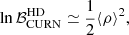
Pulsar timing srray (PTA) collaborations gather high-precision timing measurements of pulsars, with the aim of detecting gravitational wave (GW) signals. A major challenge lies in the identification and characterisation of the different sources of noise that may hamper their sensitivity to GWs. The presence of time-correlated noise that resembles the target signal might give rise to degeneracies that can directly impact the detection statistics. In this work, we focus on the covariance that exists between a ‘chromatic’ dispersion measure (DM) noise and an ‘achromatic’ stochastic gravitational wave background (GWB). The term ‘chromatic’ associated with the DM noise means that its amplitude depends on the frequency of the incoming pulsar photons measured by the radio telescopes. Multi-frequency coverage is then required to accurately characterise its chromatic features and when the coverage of incoming frequency is poor, it becomes impossible to disentangle chromatic and achromatic noise contributions. In this paper, we explore this situation by injecting realistic GWB into 100 realisations of two mock versions of the second data release (DR2) of the European PTA (EPTA), characterised by different types of frequency coverage. The first dataset is a faithful copy of DR2, in which the first half of the data is dominated by only one frequency channel for the observations; the second one is identical, except for a more homogeneous frequency coverage across the full dataset. We show that for 91% of the injections, a better frequency coverage leads to an improved statistical significance (≈1.3 dex higher log Bayes factor on average) of the GWB and a better characterisation of its properties. We propose a metric to quantify the degeneracy between DM and GWB parameters. We show that it is correlated with a loss of significance for the recovered GWB, as well as with an increase in the GWB bias towards a higher and flatter spectral shape. In the second part of the paper, this correlation between the loss of GWB significance, the degeneracy between the DM and GWB parameters, and the frequency coverage is further investigated using an analytical toy model.
Key words: gravitational waves / methods: data analysis / pulsars: general
© The Authors 2025
 Open Access article, published by EDP Sciences, under the terms of the Creative Commons Attribution License (https://creativecommons.org/licenses/by/4.0), which permits unrestricted use, distribution, and reproduction in any medium, provided the original work is properly cited.
This article is published in open access under the Subscribe to Open model. This email address is being protected from spambots. You need JavaScript enabled to view it. to support open access publication.
1. Introduction
Pulsar timing arrays (PTAs; Foster & Backer 1990) exploit the exquisite rotational stability of millisecond pulsars to search for gravitational waves (GWs). Indeed, high precision timing measurements of millisecond pulsars provide us with datasets that are sensitive enough to measure perturbations of the curvature of space-time due to the passage of GWs at nano-hertz (nano0Hz) frequencies. In this band, a stochastic GW background (GWB) is expected to be produced by a population of supermassive black hole binaries (SMBHBs; Rajagopal & Romani 1995; Jaffe & Backer 2003; Wyithe & Loeb 2003; Sesana et al. 2008) or by a number of physical processes occurring in the early Universe, from inflation to phase transitions, from scalar perturbations to domain walls and many more (see Caprini & Figueroa 2018; Afzal et al. 2023; EPTA and InPTA Collaboration 2024, and references therein). Last year, the European PTA (EPTA) collaboration with the Indian PTA (InPTA) collaboration (EPTA and InPTA Collaboration 2023a), North American Nanohertz Observatory for Gravitational Waves collaboration (NANOGrav; Agazie et al. 2023a), Parkes PTA collaboration (PPTA; Reardon et al. 2023), and the Chinese PTA collaboration (CPTA; Xu et al. 2023) reported evidence of the presence of a GWB-like signal in their dataset at a 2-to-4σ significance (depending on the dataset), effectively opening up the nano-Hz GW sky.
Pulsars are monitored in the radio-frequency band where a series of times of arrival (TOAs) of pulses are extracted from the raw data, at given epochs. Overall, PTA datasets are made up of timing residuals δt that are obtained by subtracting a best-fit timing model (TM) to the observed TOAs (e.g. Edwards et al. 2006; EPTA and InPTA Collaboration 2023c). The TM is able to predict the TOAs at the Solar System barycentre (SSB) by taking into account every physical process that occurs between the emission and reception of the pulses that can be deterministically modelled (i.e. pulsar spin-down, Einstein delay, Shapiro delay, ...). The timing residuals are made up of the difference between the observed TOAs and the TM predicted TOAs. Any feature that is not modelled by the TM will still be present in δt. These include stochastic processes that cannot be modelled by deterministic functions and (possibly) a GWB. As a result, data analysis pipelines have been developed to simultaneously fit for putative GW signals and pulsar noises in the data (Agazie et al. 2023b; EPTA and InPTA Collaboration 2023b),
Extracting a GW signal from PTA data and properly assessing its significance is no easy task, as pulsar observations suffer from a myriad of subtle stochastic noise sources (e.g. Cordes 2013; Tiburzi et al. 2016). Since a GWB produces a stochastic time correlated signal (i.e. a stochastic red signal), any noise with the same statistical properties can blend with it, affecting its recovery. The two main components of time-correlated noise are: (i) the red noise (RN): due to stochastic variations of the pulsar spin rate (e.g. Shannon & Cordes 2010) and (ii) the dispersion measure (DM) noise: due to stochastic variations of the electron density in the interstellar medium, interacting with the pulses along the line of sight (e.g. Cordes et al. 2016). Each of these physical phenomena can be recognised in PTA data by its peculiar properties. The GWB is common to all pulsars and achromatic (i.e. it does not depend on the observing radio frequency). It also features a quadrupolar spatial correlation pattern depending on the pulsars’ angular separation (Hellings & Downs 1983). RN is also achromatic, but its spectrum can vary from pulsar to pulsar and no inter-pulsars spatial correlation is expected. In addition, DM noise is expected to be specific to each pulsar with no spatial correlations, but it is chromatic, with an amplitude that is square inversely proportional to the frequency, ν, of the observed photon (e.g. You et al. 2007). Therefore, the three contributions can be in principle easily separated by a PTA with a large number of pulsars with high quality timing data, uniformly distributed in the sky and monitored in a wide radio-frequency band. Unfortunately, none of these conditions is fully met by current PTAs: current GWB evidence is dominated by just a handful of pulsars (see Speri et al. 2023). Furthermore, observing frequency coverage is scant, especially for data collected with legacy pulsar instruments, which are the oldest data.
In particular, DM noise can be problematic since its variation can be orders of magnitude higher than that of the GWB and it typically affects all the pulsars. Failing to model it properly can therefore cause significant leakage into RN and GWB, eventually compromising the GWB recovery. In order to characterise the DM noise, multi-frequency observations are required. This is the main reason why PTAs have been striving to expand the frequency coverage of their receivers and to devise new techniques to produce TOAs from wide band observations (Liu et al. 2014; Pennucci et al. 2014). Since the observations are performed using different radio-frequency channels, the timing residuals can be divided into several observation frequencies. In that sense, a PTA dataset is not only a one-dimensional (1D) data stream but, rather, a two-dimensional (2D) surface of timing residuals on the frequency ν and TOA t plane. However, as mentioned above, this surface is often not uniformly covered, as it was the case for the second EPTA data release (EPTA DR2; EPTA and InPTA Collaboration 2023c), in which the first half of the data is dominated by essentially only one observation frequency. This can introduce degeneracies between different noise components, corrupting the recovery of the GWB. Indeed, this might be one of the reasons why the GWB evidence in EPTA DR2 drops when the first half of the data is also included in the analysis (EPTA and InPTA Collaboration 2023a); this is despite the fact that we expect the GWB evidence to increase with increasing observation time.
It is therefore of primary interest to study the relation between observation frequency coverage, DM mis-modeling and GWB detection and parameter estimation. To this end, in this paper we construct two sets of synthetic PTA datasets mimicking the 24.8 years of observations collected in the EPTA DR2. One set is a faithful copy of DR2, featuring a single frequency channel in the first half of the data; the second one is identical except for the fact that observations are evenly distributed across the different frequency channels. We injected a realistic mock GWB from a cosmic population of SMBHBs (e.g. Rosado et al. 2015) and make use of standard Bayesian analysis techniques to extract the signal from the data. We demonstrate that the absence of adequate frequency coverage is detrimental to GWB recovery and parameter estimation, which has important implications for interpreting the EPTA DR2 results (EPTA and InPTA Collaboration 2023a) for forecasting PTA sensitivities (Rosado et al. 2015; Taylor et al. 2016; Speri et al. 2023) and for planning future PTA observations (e.g. Lee et al. 2012; Lam 2018).
The paper is organised as follows. In Sect. 2 we present the EPTA data (EPTA and InPTA Collaboration 2023b,c), we explain how realistic simulations of it featuring different levels of frequency coverage are generated, and we introduce the models and statistical tools used in the subsequent analysis. In Sect. 3, using these realistic simulations, we show the existence of a significant correlation between the DM-GWB and RN-GWB degeneracy and the GWB evidence and parameter estimation, and we present an analytical toy model that qualitatively explains the observed correlations. Finally, we summarise our main findings and draw our conclusions in Sect. 5.
2. Simulations and analysis tools
We investigate the impact of the observing frequency coverage on the detection significance and parameter estimation of the observed GWB by means of realistic simulations of PTA datasets. The simulations intend to reproduce the real EPTA DR2 dataset by using the same epochs TOAs, observation frequencies, and noise properties as described in EPTA and InPTA Collaboration (2023b,c). We first generate pulsar data with only white noise (WN) and inject stationary RN and DM noise. Then, a realistic GW background is added by injecting a large number (∼120 k) of individual GW sources taken from SMBHB population simulations (Sesana 2013; Rosado et al. 2015).
2.1. Real reference dataset
The dataset we took as a reference is the EPTA DR2full, which consists of 24.8 years of observation (EPTA and InPTA Collaboration 2023c), 25 pulsars, stationary noise, RN, and DM. EPTA data are taken from the major European radio telescopes: Effelsberg 100-m radio telescope (EFF) in Germany, 76-m Lovell Telescope, and Mark II Telescope at Jodrell Bank Observatory (JBO) in the United Kingdom, along with the large radio telescope operated by the Nançay Radio Observatory (NRT) in France, 64-m Sardinia Radio Telescope (SRT) operated by the Italian National Institute for Astrophysics (INAF) through the Astronomical Observatory of Cagliari (OAC), and Westerbork Synthesis Radio Telescope (WSRT) operated by ASTRON, the Netherlands Institute for Radio Astronomy. These telescopes also operate together as the Large European Array for Pulsars (LEAP), which gives an equivalent diameter of up to 194 m (Bassa et al. 2016). Contemporary measure from multiple telescopes allows us to have multi-frequency observations in a large frequency band, covering the range 323 MHz–4857 MHz. However, this large frequency band is mainly present in the second half of the data, while the first 10–15 years of observations are strongly dominated by measurements in only one narrowband, around 1400 MHz. Therefore, the frequency coverage is very inhomogeneous, especially on the pulsars with the longest observation time spans.
2.2. Simulation of a realistic PTA dataset
Here, we give a brief description of how the simulated datasets are produced. We simulated two copies of the EPTA DR2full dataset: the first reproduces the same frequency channel distribution as the real dataset, the second has an even distribution of the radio frequency channels across the entire time span of observation. The simulation pipeline starts by reproducing the main properties of the observation epochs (the observation time, the number of observations and the cadence) of each pulsar. To reproduce the true cadence of the TOAs, we have chosen to divide the data into five equal intervals and then reproduce the average cadence in each interval. This method allows us to reproduce the variability of the cadence over time and the large gaps that are present in the TOAs of some pulsars. We then assigned an observation frequency to each epoch. We generated two different sets of simulations by assigning different observation frequencies:
-
DR2full, where we assign to each simulated epoch the same radio frequency that appears in the real dataset;
-
DR2FC, where we redistribute the observation frequencies at each epoch. The new radio frequencies are uniformly chosen among the actually observed frequencies for that pulsar.
Together with the observation frequency, the corresponding observatory, backend and timing error are also associated to the epoch1, changing the number of the epochs per backends changes the total RMS of the pulsars’ residuals. However, on average, RMS stays within 1.2 times the value of DR2full RMS. Data are then generated using the libstempo package (Vallisneri 2020), assuming the TM in EPTA and InPTA Collaboration (2023c). The same package is used to inject the three components of the noise budget: WN, RN, and DM variations, as we describe next.
2.3. Simulating stationary Gaussian noise
The three noise components used in this paper are WN, RN, and DM noise. They are all stationary Gaussian processes, with the difference that WN is not correlated in time, whereas RN and DM are time-correlated signals. All noise processes n(t) are described in the time domain by their covariance matrix ⟨n(ti)n(tj)⟩. Since WN is uncorrelated in time, its covariance matrix is diagonal, with the elements given by
 (1)
(1)
where σTOA is the errorbar associated with each TOA according to the template fitting errors, EFAC accounts for the TOA measurement errors, and EQUAD accounts for any putative additional source of WN. EFAC, and EQUAD are specific to each observing backend. This model simply means that TOAs affected by the WN process are Gaussian distributed around the value predicted by the TM, where σi is the width of the Gaussian. Time-correlated signals are modelled as a combination of sine and cosine basis terms weighted by normally distributed coefficients (van Haasteren & Vallisneri 2014): for a noise n(t) evaluated at time ti with power spectral density (PSD) S(f) evaluated at frequencies fk, we have
 (2)
(2)
with Xk, Yk ∼ 𝒩(0, 1), Δfk = fk + 1 − fk, νref a reference frequency (here set to 1.4 GHz), νi the observation frequency corresponding to ti and id the chromatic index. To generate one realisation of the noise, n, we randomly drew coefficients Xk, Yk from their associated normal distribution to obtain the Fourier coefficients associated with frequency, fk. The covariance matrix corresponding to this kind of noise process is
 (3)
(3)
where the chromatic index id determines the frequency dependence of the noise. For the achromatic noise, id = 0, whereas for the DM noise, id = 2.
In Fig. 1, a comparison between real and simulated data is shown for pulsar PSR J0751+1807. In Fig. 2, a comparison between the frequency coverage of DR2full and DR2FC is shown for pulsar PSR J0751+1807.
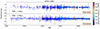 |
Fig. 1. Comparison between real data from EPTA-DR2full (top panel) and simulated data (bottom panel) for pulsar PSR J0751+1807. |
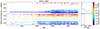 |
Fig. 2. Frequency distribution of the TOAs as a function of the observation epochs. The top panel shows the simulated DR2full-like dataset, the bottom panel shows the DR2FC-like (same epochs as DR2full, but with homogeneous distribution of observation frequencies among epochs) dataset. The histograms on the right show the distribution of the number of observations across frequencies. |
2.4. Simulation of a realistic GWB
To simulate an astrophysical GWB produced by SMBHBs, the injection pipeline starts from a population of circular SMBHBs, computes the variations induced by each binary in each pulsar TOAs and then sums these delays in the time domain. A SMBHB population is characterised by the number of emitting sources per unit redshift, mass, and frequency of d3N/(dzdℳdfr); therefore, a list of binaries can be constructed as a random sample from the numerical distribution d3N/(dzdℳdfr), which is obtained from the observation-based models described in Sesana (2013) and Rosado et al. (2015). With this method, hundreds of thousands of SMBHB populations can be obtained, which are in agreement with current constraints on the galaxy merger rate, the relation between SMBHs and their hosts, the efficiency of SMBH coalescence, and the accretion processes following galaxy mergers. The power spectrum produced by a population of SMBHBs can be computed as (Rosado et al. 2015):
 (4)
(4)
where fi is the central frequency of the bin Δfi, and the sum runs over all the binaries for which the observed frequency fr/(1 + z)∈Δfi, where fr is the GW frequency in the binary rest frame and, therefore, fr/(1 + z) is the observed frequency. Then, hj(fr) is the strain of each GW signal, given by
 (5)
(5)
where ℳ is the binary chirp mass, ı the orbit inclination angle, a(ı) = 1 + cos2ı, b(ı) = − 2cosı, and d(z) is the comoving distance of the source, computed as
 (6)
(6)
where the assumed cosmology is the Λ cold dark matter model and the set of cosmological parameters chosen is (H0,Ωm,ΩΛ) = 70 km s−1 Mpc−1, 0.3,0.7).
Since the binaries considered here are circular, their GW emission is fully described by eight parameters: ℳ, fr, and z are generated according to the observationally based model described above, while the inclination angle, ı, polarisation angle, ψ, initial phase, Φ0, and sky location (θ, ϕ) are randomly generated from uninformative distributions: cosı∈Uniform(−1, 1), ψ ∈ Uniform(0, π), ϕ0 ∈ Uniform(0, 2π), cos θ ∈ Uniform(−1, 1), and ϕ ∈ Uniform(0, 2π).
Once these eight parameters have been generated for each binary in the population, the variations induced in each pulsar are evaluated according to Ellis (2013), taking into account both the Earth and pulsar terms. They are then all summed to give the total delay induced in each pulsar by the GWB.
For the purpose of this paper, only one GWB realisation is used, which corresponds to the spectrum shown in Fig. 3. The GWB realisation is chosen such that the spectrum, if expressed in the power law taking the form
 (7)
(7)
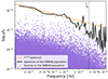 |
Fig. 3. Characteristic strain spectrum of the injected GWB. Purple stars are the contributions to the spectrum of all the SMBHBs in the population. The black solid line is the total power spectrum in each frequency bin, where the frequency bins start at f = 1/Tobs and have width Δf = 1/Tobs with Tobs = 24.8 yr. As reference, the ideal spectrum with slope −2/3 and amplitude at the reference frequency of 1 yr−1AGW = 2.4 × 10⁻¹⁵ is shown by the dashed orange line. |
has a slope α ∼ −2/3 at the lowest frequencies, which is the value expected for an ideal GW-driven population of circular binaries, and a nominal amplitude of ∼2.4 × 10⁻¹⁵, which is consistent with the value inferred from EPTA DR2new (EPTA and InPTA Collaboration 2023a).
2.5. Data analysis
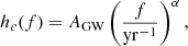
When analysing the data, we assumed Gaussian and stationary noise, and used a Gaussian likelihood. In PTA data analysis, it is customary to marginalise over first order errors of TM parameters (van Haasteren & Vallisneri 2014). The marginalisation is performed analytically and gives a TM marginalised expression of the likelihood of the form
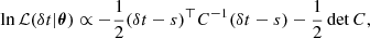 (8)
(8)
where  , and C = Caδab + ChΓab is the covariance matrix. In the latter, Ch characterises the achromatic common RN, spatially correlated between pulsars following the Hellings-Downs correlation pattern (Hellings & Downs 1983)
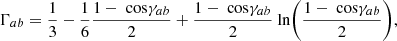 (9)
(9)
with γab as the angular separation between the pulsars in the pair ab. Then, Ca represents the noise present in pulsar a and can be written as
 (10)
(10)
where σi is the level of WN at ti, CRN is the achromatic RN, and CDM the DM noise. Here, CRN and CDM are given by Eq. (3), respectively with id = 0 and id = 2. It is usually assumed that these two noise components have power-law spectra (EPTA and InPTA Collaboration 2023b) with an amplitude and spectral index that have to be characterised for each pulsar. This complicates the task of fitting for a GWB since we also expect the latter to follow a power-law (see Eq. (7)). Thus, the covariance between noise and signal can be significant.
When performing Bayesian analysis, we updated our prior knowledge on parameters by multiplying the likelihood with the prior probability distribution π(θ) for our parameters θ. The resulting probability is the posterior probability p(θ|δt),
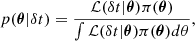 (11)
(11)
expressing the probability of measuring θ given the timing data δt. The normalisation factor, ∫ℒ(δt|θ)π(θ)dθ, is the Bayesian evidence, which is used to perform model comparison: the Bayes factor (ℬ) between two models 1 and 2 is given by the evidence of model 1 divided by the evidence of model 2:
 (12)
(12)
For the purpose of the analysis presented here, model 1 corresponds to an HD-correlated common red noise (which is the signature of a background that is gravitational in origin) and model 2 to a common, but uncorrelated, red noise.
3. Results
In this section, we show the results of the analyses performed on the two realistic datasets described in Sect. 2.2: (i) DR2full, which is a copy of the real EPTA dataset and (ii) DR2FC, which has the same observation epochs as DR2full but with a homogeneous coverage of the observation frequencies across the whole time of observation, Tobs. A comparison between simulated DR2full and DR2FC frequency coverage is shown in Fig. 2 for pulsar J0751+1807. For both cases, we generated 100 datasets, each containing the same GWB signal (whose spectrum is shown in Fig. 3), but featuring 100 different noise realisations.
3.1. Impact of the frequency coverage on the Bayes Factor
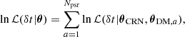
For the two types of datasets, we computed the ℬ that compares a model with a common uncorrelated red noise (CURN) and an HD-correlated common red noise (HD) through the product space method implemented in ENTERPRISE_EXTENSIONS. The  value indicates whether the dataset prefers an HD-correlated signal or a common process with no correlations. Together with the posterior distributions of the common red noise (CRN) parameters (which are the slope γ and the amplitude A of the power spectrum), the parameters of individual pulsars RN and DM noise are sampled. The WN parameters are fixed to the injected values. Therefore, the dimensionality of the posterior distribution is 64, including 62 noise parameters, and 2 GWB signal model parameters.
In the left panel of Fig. 4, the distribution of  obtained from the 100 realisations of noise is shown for DR2full and DR2FC. Let us highlight the fact that the value of
  obtained with the real DR2full is 4 (EPTA and InPTA Collaboration 2023a), which is well within the 68% C.I. of the distribution obtained with the realistic DR2full simulations,
  . This is an indication that the simulations are capturing the main features of the real data.
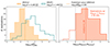 |
Fig. 4. Distributions of the Bayes factor values obtained with the two sets of simulations. Left panel: Distribution of log |


Focusing now on the comparison between the two datasets, we can conclude that the case with the better frequency coverage – DR2FC – gives significantly higher values of  with respect to DR2full datasets. Indeed, in 91% of the cases DR2FC gives better results than DR2full, with the same noise realisation. The average ratio between the DR2FC and DR2full
 is ∼20; thus, the average enhancement of the significance of signal recovery is more than one order of magnitude (see right panel of Fig. 4).
3.2. Correlation between BF and constraints on the noise parameters
In this section, we investigate a possible reason for the increase in the  due to the better frequency coverage. It is expected that a better frequency coverage improves the recovery of the DM parameters and helps to more easily disentangle this process from the achromatic RN. Indeed, the shape of the posterior distributions of the DM parameters (see Fig. 5) confirms this hypothesis: with a poor frequency coverage (DR2full), there is a strong degeneracy between the DM parameters and the CRN parameters, which is shown by the L-shape of the posterior distributions. When the coverage is improved (DR2FC), the long tails of the L-shape distributions disappear and the DM parameters are well constrained. In order to quantify the degeneracy of the CRN posterior distributions and the individual pulsars noise posterior distributions, we chose the following approach:
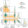 |
Fig. 5. Posterior distributions of pulsar PSR J1024-0719 individual noise and CRN parameters. Distributions obtained with one realisation of the DR2full-like dataset are shown in orange, while distributions obtained with the same realisation of the DR2FC-like dataset are shown in green. Black squares are the injected values. JSD values and Bayes factors for both datasets are reported in the top right (see text for full description). |
-
For each individual noise, we select the 2D distribution of log10ADM/RN and log10ACRN.
-
For each of these 2D posterior distributions, we generate a bivariate Gaussian distribution with same mean and covariance matrix. Then, we generate from that Gaussian distribution a number of samples equal to the 2D posterior distribution of interest.
-
We compare each generated Gaussian distribution with its parent posterior distribution by evaluating the Jensen-Shannon divergence (JSD; Nielsen 2019) between the two samples. The JSD measures the similarity between two distributions. It is symmetrical and bound between 0 and ln(2). If the JSD is high, it means that our 2D distribution is not well approximated by a bivariate Gaussian: this non-similarity is due to significant tails that characterise a degenerate, L-shaped distribution.
The effectiveness of this test depends on the assumption that the posterior distributions are either covariate Gaussians or L-shaped distributions and never have bimodalities or other features that would make them differ from a Gaussian, but without any degeneracy between the parameters. The validity of this assumption is not trivial a priori but, for the cases analysed in this investigation, has been empirically verified by visual inspection of the posterior distributions. An example of the application of this method is shown in Fig. 5. The DR2full degenerate distribution produces a JSD of 0.65 (we recall that the maximum is ∼0.69 = ln(2)), while the non-degenerate posterior distribution obtained with DR2FC gives JSD = 0.19.
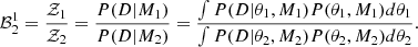
For each dataset realisation, we have 31 individual pulsar noises; therefore, we use this method to compute 31 values of JSD. To extract only one number that is representative of how much degenerate the individual noises are with the CRN, we chose to perform a weighted average of the JSD values. The weights are proportional to the contribution of each pulsar to the total GWB evidence. This contribution is evaluated exploiting the signal-to-noise ratio (S/N) defined in Rosado et al. (2015):
![Mathematical equation: $$ \begin{aligned} \mathrm{S/N}_B^2 = 2\sum _{a=1}^M\sum _{b>a}^M\frac{\Gamma _{ab}^2S^2(f)T_{ab}}{[P_a(f)+S(f)][P_b(f)+S(f)]+\Gamma _{ab}^2S^2(f)}, \end{aligned} $$](/articles/aa/full_html/2025/02/aa52805-24/aa52805-24-eq24.gif) (13)
(13)
where Pa(f) and Pb(f) are the noise spectral densities in the two pulsars a and b, while Γab is the angular correlation expected for a GWB produced by a population of SMBHBs, which is given by the Hellings and Downs curve in Eq. (9). Then, S(f) is the PSD of the GWB signal, evaluated as
 (14)
(14)
with hc2(f) given by Eq. (4). Finally, Tab is the maximum time interval over which observations from pulsar a and pulsar b overlap. This formula evaluates the S/N produced by the entire array of pulsars, thus the contribution of a single pulsar a is estimated as
![Mathematical equation: $$ \begin{aligned} \mathrm{S/N}_{B, a} = \sqrt{\sum _{b\ne a}^M\frac{\Gamma _{ab}^2S^2(f)T_{ab}}{[P_a(f)+S(f)][P_b(f)+S(f)]+\Gamma _{ab}^2S^2(f)}}. \end{aligned} $$](/articles/aa/full_html/2025/02/aa52805-24/aa52805-24-eq26.gif) (15)
(15)
Therefore, the weighted average of the JSD values is obtained as
 (16)
(16)
where the index i spans the individual noise processes and S/Ni is the contribution to the S/N of the pulsar responsible for the noise process.
Figure 6 shows the scatter plot of the weighted averaged JSD versus  for the 100 realisations of the two datasets. The distribution of (
 ) for the two datasets shows that DR2full results in lower values of log
 and higher values of
  with respect to DR2FC. We can therefore conclude that in the majority of the noise realisations the improved frequency coverage does indeed reduce the degeneracy of the noise parameters with the GWB parameters; and that this reduction in degeneracy is accompanied by an increase in the
  , implying that there is a significant correlation between the
  and the degeneracy between the individual pulsar noise and the CRN.
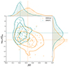 |
Fig. 6. Scatter plot of the weighted average JSD (representing how degenerate the individual noise parameters are with the CRN parameters) versus log |


3.3. Impact of the frequency coverage on the GWB parameter estimation
We then used the same two datasets – DR2full and DR2FC – to investigate the effect of frequency coverage on the recovery of the GWB parameters. The results obtained with the 100 realisations of DR2full (quoting the median and the 68% C.I.) are: log for the amplitude and
 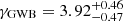 for the slope of the GWB. Therefore, as for the Bayes factor, the amplitude and slope obtained from the real DR2full analysis (log
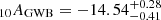 and
and 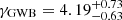 ; EPTA and InPTA Collaboration 2023a) are within the 68% C.I. obtained from our simulated datasets. From Fig. 7, it can be seen that the recovered GWB is on average higher and flatter than the injected background (log10AGWB ∼ −14.66, γGWB ∼ 4.33) and the injected values are not even on the eigen-diagonal of the distribution, but slightly below it; in fact, the injected value is not within the 90% C.I. of the 2D posterior distribution, while the recovered amplitude is (on average) higher than the injected value.
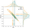 |
Fig. 7. Median of the posterior distributions of log10AGWB and γGWB obtained with the 100 realisations of DR2full (orange) and DR2FC (green). Dashed lines show the median of the 1D distributions, and the black solid line is the injection. Histograms and smoothed distributions on the top and right side of the plot represent the marginalised posterior distributions of the parameter recovery procedures. |
Figure 8 shows the weighted average JSD and the recovery of the GWB parameters for the 100 realisations of DR2full. For both parameters, there is a correlation between the recovered value and the average JSD with a significance greater than 5σ. It is a positive correlation in the case of the GWB amplitude,  , and a negative correlation in the case of the GWB slope,
 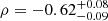 . This means that the more degenerate the individual noise parameters are with the GWB parameters, the flatter and higher is the recovered background with respect to the injection.
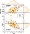 |
Fig. 8. Weighted average JSD versus GWB amplitude (top panel) and the GWB slope (bottom panel) for the 100 simulated DR2full datasets. In each panel, dashed lines correspond to the mean of the distributions, dotted dashed lines are the eigen-diagonals of the distributions, showing a strong correlation between the weighted average JSD and the recovered value of the two GWB parameters. Black solid horizontal lines are the injected values (taking in mind that the signal injected has not a perfect power-law spectrum). The error bars represent the typical size of the 68% C.I. of the posterior distributions. Histograms and smoothed distributions on the top and right side of the plot represent the marginalised posterior distributions of the corresponding quantities. |
We note, however, that even at low values of  , where the L-shape is not significant, the distribution of the recovered parameters is not centred on the injected values. This means that the degeneracy is not the only factor responsible for the bias in the recovery of the GWB parameters. This is consistent with the fact that the bias in the recovery is not solved by the improvement in the frequency coverage: the recovered values obtained with DR2FC, indeed, are also clustered at higher amplitude values and lower slope values with respect to the injection (see Fig. 7). Nevertheless, the bias is slightly reduced in this case, with respect to DR2full. The main difference between the recoveries obtained with the two datasets, which can be seen in Fig. 7, is the width of the distributions: the one obtained with DR2FC is much narrower because the noise is better modelled in this case and, therefore, there is less of a dependence on the particular realisation of noise.
The residual bias can be due to the fact that the frequency coverage of DR2FC is still characterised by a limited bandwidth and does not lead to a zero degeneracy (as can be clearly seen from Sect. 3.2). However, it should also be taken into account the fact that there is a mismatch between the power-law template used in the recovery and the spectrum of the realistic injected population (see Fig. 3); this mismatch can lead to a bias in the GWB parameters recovery, as investigated in Valtolina et al. (2024). Indeed, the minimum of the EPTA DR2 sensitivity corresponds to the first two bins, which are therefore expected to contribute most to the recovery. As can be seen in Fig. 3, even though the whole spectrum is well described by a f−2/3 power-law, the first two bins seem to slightly deviate from this slope, corresponding to a higher and flatter spectrum.
4. Understanding the RN-DM degenerate likelihood: A toy model
To gain a better insight into the results obtained in the previous section, we built a toy model to mathematically describe how the RN-DM degeneracy affects the PTA likelihood function and the recovery of the GWB signal. We started by considering a pulsar with timing residuals, δt, containing only WN, RN, and DM noise. The pulsar was observed for NE epochs with Nν frequency channels per epoch. For simplicity, we treated the RN and DM as single frequency deterministic signal to allow for a straightforward maximum likelihood calculation. We defined the RN basis, F, and the DM basis, FDM, at times, t, and frequencies, ν, as
![Mathematical equation: $$ \begin{aligned} F = [\sin (2\pi f \boldsymbol{t}), \cos (2\pi f \boldsymbol{t})];\,\,\, F_{\rm DM} = \left(\frac{\nu _{\rm ref}}{\boldsymbol{\nu }}\right)^2 F, \end{aligned} $$](/articles/aa/full_html/2025/02/aa52805-24/aa52805-24-eq44.gif) (17)
(17)
so that
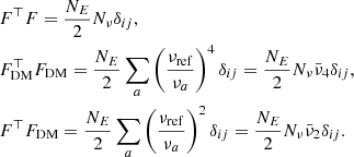 (18)
(18)
For a pulsar with RN, DM, and WN, the timing residuals are
 (19)
(19)
where n ∼ 𝒩(0, σ) is the Gaussian WN, and cRN and cDM are the true values for RN and DM amplitude, respectively. In the following, we consider that we are in the RN dominated regime so we can neglect WN n in the timing residuals. We write the likelihood as:
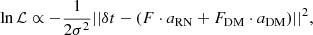 (20)
(20)
where ||y||2 = y⊤y. We can then investigate two separate situations, as detailed below.
4.1. The completely degenerate case
If all ν = νref, we have F = FDM, which yields
 (21)
(21)
In that case, aRN and aDM are completely degenerate parameters of the model since they have the same effect on the likelihood. Consequently, trying to find their maximum likelihood value gives an infinite number of solutions and they cannot be constrained. The maximum likelihood lies around the line where aRN = x(cRN + cDM) and aDM = (1 − x)(cRN + cDM), where x = [0, 1] is a real number. This produces the typical L-shaped distribution that we find in Fig. 9.
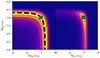 |
Fig. 9. Example of degenerate likelihood. The true value of the parameters is marked with the green cross. Left panel: Completely degenerate case ν = νref, in which RN and DM cannot be distinguished. The dashed line shows the degenerate maximum likelihood behaving as y ∝ 1 − x in log-scale. Right panel: Same likelihood with ν ≠ νref. The degenerate tails are less pronounced and the maximum likelihood lies around the true value of parameters. |
The left tail corresponds to the regime where aRN accounts for all the noise (x ≈ 1), while aDM ≈ 0 and the right tail corresponds to the regime where aDM accounts for all the noise (x ≈ 0), while aRN ≈ 0.
4.2. The non-degenerate case
If ν ≠ νref, we have F ≠ FDM, which yields
 (22)
(22)
Once F and FDM are disentangled, the maximum likelihood values of parameters aRN and aDM represent the true values cRN and cDM. Nevertheless, the tails of the previously introduced L-shape do not disappear. In fact, if the distribution of frequencies νa is very narrow and centred on the reference frequency νref, we are still in the degenerate case. We estimate the significance of each tail by setting aRN = 0 or aDM = 0 and finding the maximum likelihood for the remaining free parameters  . We have
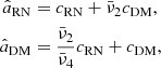 (23)
(23)
and the corresponding maximum likelihoods
![Mathematical equation: $$ \begin{aligned} \begin{aligned} \ln \mathcal{L} (\delta t | \hat{a}_{\rm RN})&\propto -\frac{N_\nu }{2\sigma ^2} \left[ \bar{\nu }_4 - \bar{\nu }^2_2 \right] c_{\rm DM}^2 = -\frac{N_\nu }{2\sigma ^2} \sigma ^2_\nu c_{\rm DM}^2, \\ \ln \mathcal{L} (\delta t | \hat{a}_{\rm DM})&\propto -\frac{N_\nu }{2\sigma ^2} \left[ 1 - \frac{\bar{\nu }_2^2}{\bar{\nu }_4} \right] c_{\rm RN}^2 = -\frac{N_\nu }{2\sigma ^2} \sigma ^2_\nu \frac{c_{\rm RN}^2}{\bar{\nu }_4}. \end{aligned} \end{aligned} $$](/articles/aa/full_html/2025/02/aa52805-24/aa52805-24-eq52.gif) (24)
(24)
The significance of each tail depends on the amplitude of the noise component it is trying to fit and scales as the variance, σν, of the inverse squared frequencies, ν, per epoch. We can isolate from the previous expressions a coefficient that is only a function of the frequency coverage and quantifies the degeneracy between RN and DM,
 (25)
(25)
which is bound between 0 and 1. If ν = νref, d(RN|DM) = 1, if not: 0 < d(RN|DM) < 1.
In Fig. 10, we verify the relationship between the coefficient d(RN|DM) and the JSD metric defined in Sect. 3.2 characterising the degeneracy from the posterior distribution. For decreasing values of d(RN|DM), we have decreasing values of JSD.
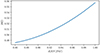 |
Fig. 10. JSD as a function of d(RN|DM) estimated using the toy model. |
4.3. Parameter estimation and S/N
We showed that the degeneracy between RN and DM will bias parameter estimation. In the weak signal regime, the optimal S/N for a GWB with HD correlations is (Vigeland et al. 2018):
![Mathematical equation: $$ \begin{aligned} \rho _{HD} = \frac{\sum _{ab} \delta t_a^\top C_a ^{-1} S_{ab} C_b^{-1} \delta t_b}{\left[ \sum _{ab} \text{ tr} \left( C_a ^{-1} S_{ab} C_b^{-1} S_{ba} \right) \right]^{1/2}}, \end{aligned} $$](/articles/aa/full_html/2025/02/aa52805-24/aa52805-24-eq54.gif) (26)
(26)
where Γab is the Hellings-Downs correlation coefficient between pulsars a and b, Sh is the PSD of the GWB signal and Sa, Sb are the PSD of the noise in pulsars a and b. It is clear that an erroneous estimation of signal and noise parameters will affect the S/N.
To evaluate the influence of frequency coverage on S/N estimation, we compute the likelihood for a toy dataset of 25 pulsars containing WN, DM noise and a GWB in their residuals with 10 years of observation and a 2 weeks cadence. The GWB and DM noise spectra are modelled as a power-law with fixed spectral index γ = 3 and same amplitude. Since the level of noise is identical in each pulsar (ACRN = ADM, a = 10−14 and σ = 10−6s), we assume a factorised likelihood form (Taylor et al. 2022) where we only vary the amplitudes of CRN and DM as:
 (27)
(27)
where θCRN are the CRN parameters and the θDM, a are the DM noise parameters for pulsar a.
In this simplified configuration, we consider each lnℒ(δt|θCRN, θDM, a) to be identical and estimate it once on a 2D grid using the expression given in Eq. (8). Thus, for a given prior π(θ), we can directly produce sets of samples by first drawing θCRN from the 1D marginalised posterior distribution p(θCRN|δt) and independently drawing the θDM, a from the conditional distribution p(θDM, a|δt, θCRN). We can generate many fake PTAs, for which we only vary the frequency coverage, splitting the TOAs into five different frequency channels distributed in the L-band; namely, ν = 1 − 2 GHz. For each simulation, we compute the marginalised OS S/N using Eq. (26) and the degeneracy coefficient d(RN|DM) using Eq. (25).
The recovered S/Ns as a function of d(RN|DM) is shown in Fig. 11. The S/N shows a clear dependence on the frequency coverage. Adding higher frequency channels in our array reduces the amplitude of DM and improves the S/N (since DM varies as ν−2), while adding lower frequency channels gives a better characterisation of the latter because it is more pronounced at low ν. We can see that even for slightly improved coverage, the difference in S/N can be significant. In the weak signal regime, we can link the S/N to the ℬ through the formula (Vallisneri et al. 2023)
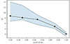 |
Fig. 11. S/N as a function of the degeneracy coefficient from 1000 simulations. The blue region represents the 1σ credible region. |
 (28)
(28)
giving a slight increase in the coverage and, therefore, in the S/N as well, leading to an exponential growth in terms of ℬ (see Fig. 12).
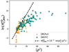 |
Fig. 12. S/N squared and ln(ℬ) for the 100 realisations of DR2full (orange) and DR2FC (green). The dashed line represents the expected relation in the weak signal regime. |
The results from the simple simulations described in this section can be compared with those from the realistic simulations: we can evaluate the HD S/N given by the 100 realisations of the two realistic datasets, DR2full and DR2FC, with the noise marginalised optimal statistic method (Vigeland et al. 2018). We can also evaluate the degeneracy coefficient d(RN|DM), which depends only on the frequency coverage σν, for the two realistic datasets. The values of HD S/N averaged over the noise realisations are ∼2.50 and ∼4.42, respectively; while the values of d(RN|DM) are ∼0.97 and ∼0.95. The average S/N ⟨ρ⟩ shown in Fig. 11 was obtained for an ideal PTA with evenly distributed data, resulting in higher values compared to realistic simulations. Nevertheless, we can compare the relative increase in the average S/N that follows an improvement in the frequency coverage from d(RN|DM) = 0.97 to d(RN|DM) = 0.95 (i.e. from DR2full to DR2FC). The ratio between DR2FC HD S/N and DR2full HD S/N is ∼4.43/2.50 ∼ 1.77 ± 0.91, while the ratio extrapolated from the ⟨ρ⟩ vs d(RN|DM) curve is 6.16/4.80 ∼ 1.29 ± 0.78. Therefore, we see that they are very compatible. Still, this good agreement is accompanied by large errors in the two estimates, due to the dependence on the noise realisation.
Even slight changes in the frequency coverage of a PTA can have a strong impact on the significance of the recovered signal. It is then fundamental to have an accurate characterisation of the DM noise to remove potential degeneracies between DM and RN. The next generation of observatories at very low frequency where the DM noise is high, such as SKA (e.g. Bhat et al. 2018), LOFAR (e.g. Kondratiev et al. 2016), Nenufar (Bondonneau et al. 2021), and Chime (Amiri et al. 2021), will provide good estimates of DM to better distinguish the latter from achromatic noise (Iraci, et al. in prep.).
5. Conclusions
Noise modelling is a cornerstone of a functioning PTA and the importance of customised noise models for each pulsar was highlighted in previous studies (Chalumeau et al. 2021). In this work, we have explored the degeneracies that may occur between the noise models and the GW signal models. In particular, we focused on the DM noise that has a chromatic dependence on the incoming photon’s frequency. The characterisation of the latter requires multi-frequency observation capabilities at the radio telescope, since having a single frequency channel of observation makes it impossible to differentiate between achromatic noise and chromatic noise.
We simulated realistic PTA datasets based on the second data release of the EPTA collaboration. This dataset is dominated by a single frequency of observation in its first half, possibly introducing biases in the estimates of the GWB signal and DM noise. We produced two versions of this dataset: (i) with the real frequency channel distribution and (ii) with a homogeneous frequency channel distribution. For each of the two datasets, we performed 100 simulations with the same realisation of GWB signal, but 100 different realisations of noise. We found that in 91% of the cases, the Bayes factor in favour of a GWB was significantly boosted by the improvement in the frequency coverage, as shown in Fig. 4, with an average value that is 20 times higher compared to the datasets mimicking EPTA DR2. This is because without proper frequency coverage, DM can easily be mis-modelled, leaking into the RN budget. Since DM affects all pulsars and can be orders of magnitude higher than RN, by leaking in the RN budget, it can give rise to a spurious common red signal that can severely interfere with the GWB recovery. The degeneracy that exists between DM and RN parameters can be observed in the 2D posterior probability distributions (see Figs. 5 and 9). We have proposed a metric to measure the amount of degeneracy based on the Jensen-Shannon divergence and show that a reduced level of degeneracy is correlated with an improved significance of the GWB (Fig. 6). Indeed, since parameter estimation is strongly affected by the observation frequency coverage, the S/N and the ℬ in favour of a GWB will deteriorate as the coverage decreases (see Fig. 11). As expected, the recovery of the GWB parameters is also strongly correlated with the degeneracy between the DM and GWB parameters. In particular, a larger degeneracy is associated with a bias of the GWB recovery towards a flatter and higher spectrum.
In conclusion, this work shows that it is not particularly surprising that a dataset with the characteristics of EPTA DR2full does not return a significant detection of a GWB with a nominal amplitude of 2.4 × 10⁻¹⁵ EPTA and InPTA Collaboration (2023a). One of the reasons for this is the highly inhomogeneous frequency coverage. It also shows that care must be taken when forecasting future PTA capabilities or when devising observing strategies to maximise the scientific potential of a PTA. Not properly taking into account the DM-RN degeneracy can lead to overoptimistic results and biased forecasts. Finally, it is of paramount importance to include in the PTA datasets data from the new generations of radio telescopes (LOFAR, Chime, SKA), with an increased frequency band, to help in distinguishing chromatic features from GW signals. Understanding the DM noise and all other chromatic features that are present in pulsar timing data is a fundamental aspect of PTAs and should be one of the priorities for the future.
The same simulation pipeline used in this paper can be exploited to investigate the difference between the results obtained with DR2full and DR2new, which is essential to assess the robustness of EPTA results. Future work will be devoted to this analysis.
Since every backend has its characteristic level of WN.
Acknowledgments
M.F. acknowledges financial support from MUR through the PRIN 2022 project ‘General Relativistic Astrometry and Pulsar Experiment’ (GRAPE, 2022-MYL2X). A.S. acknowledges financial support provided under the European Union’s H2020 ERC Consolidator Grant “Binary Massive Black Hole Astrophysics” (B Massive, Grant Agreement: 818691). The Nançay radio Observatory is operated by the Paris Observatory, associated with the French Centre National de la Recherche Scientifique (CNRS), and partially supported by the Region Centre in France. I.C., L.G. and G.T. acknowledge financial support from “Programme National de Cosmologie and Galaxies” (PNCG), “Programme National Hautes Energies” (PNHE), and “Programme National Gravitation, Références, Astronomie, Métrologie” (PNGRAM) funded by CNRS/INSU-IN2P3-INP, CEA and CNES, France. We acknowledge financial support from Agence Nationale de la Recherche (project “PTA-France”, ANR-18-CE31-0015), France.
References
- Afzal, A., Agazie, G., Anumarlapudi, A., et al. 2023, ApJ, 951, L11 [NASA ADS] [CrossRef] [Google Scholar]
- Agazie, G., Anumarlapudi, A., Archibald, A. M., et al. 2023a, ArXiv e-prints [arXiv:2306.16221] [Google Scholar]
- Agazie, G., Anumarlapudi, A., Archibald, A. M., et al. 2023b, ApJ, 951, L10 [CrossRef] [Google Scholar]
- Amiri, M., Bandura, K. M., Boyle, P. J., et al. 2021, ApJS, 255, 5 [NASA ADS] [CrossRef] [Google Scholar]
- Bassa, C. G., Janssen, G. H., Stappers, B. W., et al. 2016, MNRAS, 460, 2207 [NASA ADS] [CrossRef] [Google Scholar]
- Bhat, N. D. R., Tremblay, S. E., Kirsten, F., et al. 2018, ApJS, 238, 1 [Google Scholar]
- Bondonneau, L., Grießmeier, J.-M., Theureau, G., et al. 2021, A&A, 652, A34 [NASA ADS] [CrossRef] [EDP Sciences] [Google Scholar]
- Caprini, C., & Figueroa, D. G. 2018, Classical Quantum Gravity, 35, 163001 [NASA ADS] [CrossRef] [Google Scholar]
- Chalumeau, A., Babak, S., Petiteau, A., et al. 2021, MNRAS, 509, 5538 [NASA ADS] [CrossRef] [Google Scholar]
- Cordes, J. M. 2013, Classical Quantum Gravity, 30, 224002 [NASA ADS] [CrossRef] [Google Scholar]
- Cordes, J. M., Shannon, R. M., & Stinebring, D. R. 2016, ApJ, 817, 16 [Google Scholar]
- Edwards, R. T., Hobbs, G. B., & Manchester, R. N. 2006, MNRAS, 372, 1549 [Google Scholar]
- Ellis, J. A. 2013, Classical Quantum Gravity, 30, 224004 [NASA ADS] [CrossRef] [Google Scholar]
- EPTA and InPTA Collaboration (Antoniadis, J., et al.) 2023a, A&A, 678, A50 [CrossRef] [EDP Sciences] [Google Scholar]
- EPTA and InPTA Collaboration (Antoniadis, J., et al.) 2023b, A&A, 678, A49 [Google Scholar]
- EPTA and InPTA Collaboration (Antoniadis, J., et al.) 2023c, A&A, 678, A48 [Google Scholar]
- EPTA and InPTA Collaboration (Antoniadis, J., et al.) 2024, A&A, 685, A94 [NASA ADS] [CrossRef] [EDP Sciences] [Google Scholar]
- Foster, R. S., & Backer, D. C. 1990, ApJ, 361, 300 [NASA ADS] [CrossRef] [Google Scholar]
- Hellings, R. W., & Downs, G. S. 1983, ApJ, 265, L39 [NASA ADS] [CrossRef] [Google Scholar]
- Jaffe, A. H., & Backer, D. C. 2003, ApJ, 583, 616 [NASA ADS] [CrossRef] [Google Scholar]
- Kondratiev, V. I., Verbiest, J. P. W., Hessels, J. W. T., et al. 2016, A&A, 585, A128 [NASA ADS] [CrossRef] [EDP Sciences] [Google Scholar]
- Lam, M. T. 2018, ApJ, 868, 33 [NASA ADS] [CrossRef] [Google Scholar]
- Lee, K. J., Bassa, C. G., Janssen, G. H., et al. 2012, MNRAS, 423, 2642 [NASA ADS] [CrossRef] [Google Scholar]
- Liu, K., Desvignes, G., Cognard, I., et al. 2014, MNRAS, 443, 3752 [NASA ADS] [CrossRef] [Google Scholar]
- Nielsen, F. 2019, Entropy, 21, 485 [NASA ADS] [CrossRef] [Google Scholar]
- Pennucci, T. T., Demorest, P. B., & Ransom, S. M. 2014, ApJ, 790, 93 [NASA ADS] [CrossRef] [Google Scholar]
- Rajagopal, M., & Romani, R. W. 1995, ApJ, 446, 543 [NASA ADS] [CrossRef] [Google Scholar]
- Reardon, D. J., Zic, A., Shannon, R. M., et al. 2023, ApJ, 951, L6 [NASA ADS] [CrossRef] [Google Scholar]
- Rosado, P. A., Sesana, A., & Gair, J. 2015, MNRAS, 451, 2417 [NASA ADS] [CrossRef] [Google Scholar]
- Sesana, A. 2013, Classical Quantum Gravity, 30, 244009 [NASA ADS] [CrossRef] [Google Scholar]
- Sesana, A., Vecchio, A., & Colacino, C. N. 2008, MNRAS, 390, 192 [NASA ADS] [CrossRef] [Google Scholar]
- Shannon, R. M., & Cordes, J. M. 2010, ApJ, 725, 1607 [NASA ADS] [CrossRef] [Google Scholar]
- Speri, L., Porayko, N. K., Falxa, M., et al. 2023, MNRAS, 518, 1802 [Google Scholar]
- Taylor, S. R., Vallisneri, M., Ellis, J. A., et al. 2016, ApJ, 819, L6 [NASA ADS] [CrossRef] [Google Scholar]
- Taylor, S. R., Simon, J., Schult, L., Pol, N., & Lamb, W. G. 2022, Phys. Rev. D, 105, 084049 [NASA ADS] [CrossRef] [Google Scholar]
- Tiburzi, C., Hobbs, G., Kerr, M., et al. 2016, MNRAS, 455, 4339 [Google Scholar]
- Vallisneri, M. 2020, Astrophysics Source Code Library [record ascl:2002.017] [Google Scholar]
- Vallisneri, M., Meyers, P. M., Chatziioannou, K., & Chua, A. J. 2023, Phys. Rev. D, 108, 123007 [NASA ADS] [CrossRef] [Google Scholar]
- Valtolina, S., Shaifullah, G., Samajdar, A., & Sesana, A. 2024, A&A, 683, A201 [NASA ADS] [CrossRef] [EDP Sciences] [Google Scholar]
- van Haasteren, R., & Vallisneri, M. 2014, Phys. Rev. D, 90, 104012 [NASA ADS] [CrossRef] [Google Scholar]
- Vigeland, S. J., Islo, K., Taylor, S. R., & Ellis, J. A. 2018, Phys. Rev. D, 98, 044003 [NASA ADS] [CrossRef] [Google Scholar]
- Wyithe, J. S. B., & Loeb, A. 2003, ApJ, 590, 691 [NASA ADS] [CrossRef] [Google Scholar]
- Xu, H., Chen, S., Guo, Y., et al. 2023, Res. Astron. Astrophys., 23, 075024 [CrossRef] [Google Scholar]
- You, X. P., Hobbs, G., Coles, W. A., et al. 2007, MNRAS, 378, 493 [Google Scholar]
All Figures
|
Fig. 1. Comparison between real data from EPTA-DR2full (top panel) and simulated data (bottom panel) for pulsar PSR J0751+1807. |
| In the text | |
|
Fig. 2. Frequency distribution of the TOAs as a function of the observation epochs. The top panel shows the simulated DR2full-like dataset, the bottom panel shows the DR2FC-like (same epochs as DR2full, but with homogeneous distribution of observation frequencies among epochs) dataset. The histograms on the right show the distribution of the number of observations across frequencies. |
| In the text | |
|
Fig. 3. Characteristic strain spectrum of the injected GWB. Purple stars are the contributions to the spectrum of all the SMBHBs in the population. The black solid line is the total power spectrum in each frequency bin, where the frequency bins start at f = 1/Tobs and have width Δf = 1/Tobs with Tobs = 24.8 yr. As reference, the ideal spectrum with slope −2/3 and amplitude at the reference frequency of 1 yr−1AGW = 2.4 × 10⁻¹⁵ is shown by the dashed orange line. |
| In the text | |
|
Fig. 4. Distributions of the Bayes factor values obtained with the two sets of simulations. Left panel: Distribution of log |
| In the text | |
|
Fig. 5. Posterior distributions of pulsar PSR J1024-0719 individual noise and CRN parameters. Distributions obtained with one realisation of the DR2full-like dataset are shown in orange, while distributions obtained with the same realisation of the DR2FC-like dataset are shown in green. Black squares are the injected values. JSD values and Bayes factors for both datasets are reported in the top right (see text for full description). |
| In the text | |
|
Fig. 6. Scatter plot of the weighted average JSD (representing how degenerate the individual noise parameters are with the CRN parameters) versus log |
| In the text | |
|
Fig. 7. Median of the posterior distributions of log10AGWB and γGWB obtained with the 100 realisations of DR2full (orange) and DR2FC (green). Dashed lines show the median of the 1D distributions, and the black solid line is the injection. Histograms and smoothed distributions on the top and right side of the plot represent the marginalised posterior distributions of the parameter recovery procedures. |
| In the text | |
|
Fig. 8. Weighted average JSD versus GWB amplitude (top panel) and the GWB slope (bottom panel) for the 100 simulated DR2full datasets. In each panel, dashed lines correspond to the mean of the distributions, dotted dashed lines are the eigen-diagonals of the distributions, showing a strong correlation between the weighted average JSD and the recovered value of the two GWB parameters. Black solid horizontal lines are the injected values (taking in mind that the signal injected has not a perfect power-law spectrum). The error bars represent the typical size of the 68% C.I. of the posterior distributions. Histograms and smoothed distributions on the top and right side of the plot represent the marginalised posterior distributions of the corresponding quantities. |
| In the text | |
|
Fig. 9. Example of degenerate likelihood. The true value of the parameters is marked with the green cross. Left panel: Completely degenerate case ν = νref, in which RN and DM cannot be distinguished. The dashed line shows the degenerate maximum likelihood behaving as y ∝ 1 − x in log-scale. Right panel: Same likelihood with ν ≠ νref. The degenerate tails are less pronounced and the maximum likelihood lies around the true value of parameters. |
| In the text | |
|
Fig. 10. JSD as a function of d(RN|DM) estimated using the toy model. |
| In the text | |
|
Fig. 11. S/N as a function of the degeneracy coefficient from 1000 simulations. The blue region represents the 1σ credible region. |
| In the text | |
|
Fig. 12. S/N squared and ln(ℬ) for the 100 realisations of DR2full (orange) and DR2FC (green). The dashed line represents the expected relation in the weak signal regime. |
| In the text | |
Current usage metrics show cumulative count of Article Views (full-text article views including HTML views, PDF and ePub downloads, according to the available data) and Abstracts Views on Vision4Press platform.
Data correspond to usage on the plateform after 2015. The current usage metrics is available 48-96 hours after online publication and is updated daily on week days.
Initial download of the metrics may take a while.