| Issue |
A&A
Volume 684, April 2024
|
|
|---|---|---|
| Article Number | A206 | |
| Number of page(s) | 19 | |
| Section | Stellar structure and evolution | |
| DOI | https://doi.org/10.1051/0004-6361/202348957 | |
| Published online | 25 April 2024 | |
The intermediate neutron capture process
V. The i-process in AGB stars with overshoot
Institut d’Astronomie et d’Astrophysique, Université Libre de Bruxelles, CP 226, 1050 Brussels, Belgium
e-mail: This email address is being protected from spambots. You need JavaScript enabled to view it.
Received:
14
December
2023
Accepted:
9
February
2024
Abstract
Context. The intermediate neutron capture process (i-process) can develop during proton ingestion events (PIE), potentially during the early stages of low-mass low-metallicity asymptotic giant branch (AGB) stars.
Aims. We examine the impact of overshoot mixing on the triggering and development of i-process nucleosynthesis in AGB stars of various initial masses and metallicities.
Methods. We computed AGB stellar models, with initial masses of 1, 2, 3, and 4 M⊙ and metallicities in the −2.5 ≤ [Fe/H] ≤ 0 range, using the stellar evolution code STAREVOL with a network of 1160 nuclei coupled to the transport equations. We considered different overshooting profiles below and above the thermal pulses, and below the convective envelope.
Results. The occurrence of PIEs is found to be primarily governed by the amount of overshooting at the top of pulse (ftop) and to increase with rising ftop. For ftop = 0, 0.02, 0.04, and 0.1, we find that 0%, 6%, 24%, and 86% of our 21 AGB models with −2 < [Fe/H] < 0 experience a PIE, respectively. Variations of the overshooting parameters during a PIE leads to a scatter on abundances of 0.5 − 1 dex on elements, with 36 < Z < 56; however, this barely impacts the production of elements with 56 < Z < 80, which therefore appear to be a reliable prediction of our models. Actinides are only produced if the overshooting at the top of pulse is small enough. We also find that PIEs leave a 13C-pocket at the bottom of the pulse that can give rise to an additional radiative s-process nucleosynthesis. In the case of the 2 M⊙ models with [Fe/H] = −1 and −0.5, it produces a noticeable mixed i + s chemical signature at the surface. Finally, the chemical abundance patterns of 22 observed r/s-stars candidates (18 dwarfs or giants and 4 post-AGB) with −2 < [Fe/H] < −1 are found to be in reasonable agreement with our AGB model predictions. The binary status of the dwarfs/giants being unclear, we suggest that these stars have acquired their chemical pattern either from the mass transfer of a now-extinct AGB companion or from an early generation AGB star that polluted the natal cloud.
Conclusions. The occurrence of PIEs and the development of i-process nucleosynthesis in AGB stars remains sensitive to the overshooting parametrization. A high (yet realistic) ftop value triggers PIEs at (almost) all metallicities. The existence of r/s-stars at [Fe/H] ≃ −1 is in favour of an i-process operating in AGB stars up to this metallicity. Stricter constraints from multi-dimensional hydrodynamical models on overshoot coefficients could deliver new insights into the contribution of AGB stars to heavy elements in the Universe.
Key words: nuclear reactions / nucleosynthesis / abundances / stars: AGB and post-AGB
© The Authors 2024
 Open Access article, published by EDP Sciences, under the terms of the Creative Commons Attribution License (https://creativecommons.org/licenses/by/4.0), which permits unrestricted use, distribution, and reproduction in any medium, provided the original work is properly cited.
This article is published in open access under the Subscribe to Open model. This email address is being protected from spambots. You need JavaScript enabled to view it. to support open access publication.
1. Introduction
Understanding the chemical evolution of the Universe requires a thorough comprehension of all nucleosynthetic processes, in particular, the astrophysical sites where they take place and the various physical mechanisms taking place at their origin. The elements heavier than Fe are mostly synthesized by the slow and rapid neutron-capture processes (e.g., Arnould & Goriely 2020, for a review), which are characterized by neutron densities on the order of Nn = 105 − 1010 and Nn > 1024 cm−3, respectively. The main astrophysical sites for the s-process are asymptotic giant branch stars (AGB; e.g., Gallino et al. 1998; Herwig 2005; Cristallo et al. 2009a,b, 2011; Bisterzo et al. 2011; Karakas & Lattanzio 2014; Fishlock et al. 2014; Goriely & Siess 2018) and the helium-burning core of massive stars (e.g., Langer et al. 1989; Prantzos et al. 1990; Pignatari et al. 2008; Frischknecht et al. 2016; Choplin et al. 2018). The r-process requires a more violent environment, which could be the merging of two neutron stars (e.g., Arnould et al. 2007; Goriely et al. 2011a,b; Wanajo et al. 2014; Just et al. 2015), collapsars, or magnetorotational supernovae (Winteler et al. 2012; Nishimura et al. 2015; Siegel et al. 2019).
Other secondary neutron capture processes were identified. One of them is the so-called intermediate neutron-capture process (Cowan & Rose 1977), which is associated with neutron densities of about Nn = 1013 − 1016 cm−3, namely, in between the s- and r-processes. The existence of the i-process is supported by the observation of stars with chemical overabundances that are not compatible with the s- or the r-processes alone. Instead these stars can be explained by considering an intermediate neutron irradiation, as modeled by i-process calculations (r/s-stars, e.g., Mishenina et al. 2015; Roederer et al. 2016; Karinkuzhi et al. 2021, 2023; Mashonkina et al. 2023; Hansen et al. 2023). Some pre-solar grains may also bear the signature of i-process nucleosynthesis (Fujiya et al. 2013; Jadhav et al. 2013; Liu et al. 2014).
The i-process nucleosynthesis can develop if protons are mixed in a convective helium-burning zone (proton ingestion event or PIE). This could take place in different astrophysical sites (see Choplin et al. 2021, for a detailed list), one of which is low-metallicity low-mass AGB stars (e.g., Iwamoto et al. 2004; Cristallo et al. 2009a; Suda & Fujimoto 2010; Choplin et al. 2021, 2022a; Goriely et al. 2021; Gil-Pons et al. 2022). In such stars, the top of the convective thermal pulse encroaches on the tail of the hydrogen-rich zone. Protons are then transported downwards by convection (on a typical timescale of 1 h) and burnt on the way via 12C(p, γ)13N. The 13N isotope decays to 13C in about 10 min. At this point, the 13C(α, n)16O reaction becomes active, mostly at the bottom of the pulse, where the temperature is about 250 MK. The neutron density goes up to Nn ≃ 1015 cm−3, which triggers the i-process, and possibly the synthesis of actinides (Choplin et al. 2022b). The convective thermal pulse splits in two parts after the neutron density peak (cf. Sect. 3.5 in Choplin et al. 2022a, for a discussion about the split) and the upper part eventually merges with the convective envelope. There, the i-process products are diluted into the envelope and then expelled by the stellar winds.
In Choplin et al. (2022a, hereafter Paper III), we have shown that AGB models with Mini ≲ 3.0 and [Fe/H] ≲ −2 that do not include extra mixing (e.g., overshoot) experience PIEs (see Fig. 3 in Paper III for a more detailed view). What remains unknown is how the development of PIEs in AGB stars is affected by extra mixing, particularly overshooting. This is of importance to better assess the contribution of AGB stars to the Galactic enrichment as well as the chemical evolution of the Universe.
Hydrodynamical simulations have shown that convection extends beyond the boundary of the convectively unstable region (e.g., Freytag et al. 1996). This extra mixing can be implemented in 1D stellar evolution codes with a parametrized diffusion coefficient. One possible parametrization is expressed as follows (e.g., Freytag et al. 1996; Herwig et al. 1997):
 (1)
(1)
where z is the distance from the formal convective boundary, Dcb is the diffusion coefficient at the edge of the convective zone (as defined by the Schwarzschild criterion), fover is a free parameter controlling the efficiency of the mixing and that can be different at each convective boundary. Table 1 reports the values of fover adopted at three different convective borders by various studies. We note that Herwig et al. (2007) proposed to approximate the overshoot at the base of the convective pulse by two exponential decays (see also Battino et al. 2016), characterized by fbot, 1 = 0.01 and fbot, 2 = 0.14 (hence, the two values in Table 1). The overshoot parameters are generally calibrated based on observations. For instance, the overshoot parameter below the envelope, fenv, is determine so as to form a 13C-pocket massive enough to account for the level of surface s-process enrichment. The overshoot parameter at the bottom of the pulse, fbot, was shown to scale with the O abundance in the thermal pulse (Herwig 2000). This parameter was thus sometimes calibrated to reproduce the O abundance of observed post-AGB stars (e.g., Herwig et al. 1999; Pignatari et al. 2016; Wagstaff et al. 2020). However, Lattanzio et al. (2017) suggested that the strong buoyancy at the base of the convective pulse would lead to a small if not negligible amount of overshoot at this border, namely, fbot ≃ 0. In the recent work of Karinkuzhi et al. (2023), the observation of two r/s-stars at metallicity [Fe/H] > −1 was reported. Their abundance was suggested to originate from an AGB binary companion at [Fe/H] ≃ −0.5 that experienced a PIE. This result was obtained by considering some overshoot at the top of the convective pulse in the AGB model (ftop = 0.06) to facilitate the ingestion of protons and trigger i-process nucleosynthesis at higher mass and metallicities. The present paper details the extensive study we carried out on the impact of overshoot on the i-process in AGB stars.
Overshoot coefficients used in the literature, at the bottom of the convective envelope (fenv) at the top of the convective pulse (ftop) and at the bottom of the convective pulse (fbot).
After introducing the necessary physics of the models in Sect. 2, we scrutinize the impact of a large set of overshoot parameters during the PIE of a 1 M⊙ AGB model at [Fe/H] = −2.5 (Sect. 3). In Sect. 4, we examine the effect of a more limited set of overshoot parameters (four different ftop values), but in AGB models of various initial masses and metallicities. Section 5 is dedicated to the comparison of our models to the chemical abundances of observed stars. Our conclusions are given in Sect. 6.
2. Physical inputs of the models
The models were computed with the stellar evolution code STAREVOL (Siess et al. 2000; Siess 2006; Goriely & Siess 2018, and references therein). We considered initial masses, at the zero-age main sequence (ZAMS), of Mini = 1, 2, 3, and 4 M⊙ and metallicities in the range of −2.5 ≤ [Fe/H] ≤ 0 with the solar mixture of Asplund et al. (2009). We did not consider α-enhanced mixtures for the sake of homogeneity. Discussions on the impact of an α-enhancement on the PIE can be found in Cristallo et al. (2016) or Choplin et al. (2022a, see their Sect. 4.7 in particular) for instance. The mass loss prescription of Schröder & Cuntz (2007) is used up to the start of the AGB phase and then switched to the one of Vassiliadis & Wood (1993). As in the previous papers of this series, when the star becomes carbon rich, the opacity change due to the formation of molecules is taken into account following Marigo (2002). The mixing length parameter is set to 1.75. A network of 411 nuclei is used up to the occurrence of a PIE. When a PIE was about to start, we switched to an i-process network of 1160 nuclei, which we coupled to the transport equations. We refer to Choplin et al. (2021, 2022a), Goriely et al. (2021) for more details on the input physics. In this work, the models were computed from the ZAMS and for some models (see Table 2) up to the end of AGB phase. Nevertheless, as discussed in Sect. 4, the missing part of the AGB phase of some models is not expected to significantly affect the resulting surface chemical abundances. Convective overshoot is included from the start of the AGB phase. Details on the implementation can be found in the next section.
Properties of the computed models for the various values of ftop.
2.1. Convective overshooting
The modeling of overshooting is performed according to the prescription of Goriely & Siess (2018), where the overshoot diffusion coefficient, Dover, follows the expression
 (2)
(2)
where z* = fover Hp ln(Dcb)/2 is the distance over which mixing occurs, Dmin is the value of the diffusion coefficient at the boundary, z = z*, and p is a free parameter controlling the slope of the exponential decrease of Dover with z (see Fig. 1 of Goriely & Siess 2018, for an illustration of the effect of the parameter, p). Below Dmin, we assume that Dover = 0. The fover parameter corresponds to the radial extent over which the mixing takes place. We note that the original prescription of Herwig et al. (1997) is recovered if Dmin = 1 cm2 s−1, fover = 0.02, and p = 1. We refer to Goriely & Siess (2018, especially Sect. 2) for more details. In the present study, when not mentioned otherwise, we adopt the default values of Dmin = 1 cm2 s−1 and p = 1.
3. Impact of overshoot in a 1 M⊙ [Fe/H] = −2.5 AGB model
In this section, we discuss the impact of overshoot during the PIE of a 1 M⊙, [Fe/H] = −2.5 AGB model. We consider overshooting above (ftop) and below (fbot) the convective pulse, as well as below the convective envelope (fenv). We also look at the impact of the Dmin and p parameters (cf. Eq. (2)). In total, 30 AGB models during a given PIE were computed. These calculations being computationally expensive, we use the same dilution procedure as in Martinet et al. (2024, cf. Sect. 3.1) to determine the surface composition after the PIE, which is briefly recalled below.
3.1. The dilution procedure
In this procedure, models are stopped when the convective pulse splits, that is, just after the neutron density peak. The final surface abundances are predicted by diluting the chemical abundances in the homogenized pulse with those of the envelope. As discussed in Martinet et al. (2024), this method leads to a very accurate estimate of the final surface abundances with the exception of Li, C, and N. In this work, we once again checked the accuracy of this procedure by computing several models up to the merging of the pulse with the envelope. When comparing the final abundances to the ones derived from the dilution procedure, a maximal deviation of about 10% is noted. This procedure is only used in the present Sect. 3 to analyze the impact of the various overshoot parameters.
3.2. The impact of overshooting above the convective thermal pulse
We first included the overshoot at the top of all convective boundaries. Eight values of ftop were considered, from 0 to 0.2, with Dmin = 1 cm2 s−1 and p = 1. Without overshoot or with small values of ftop, protons are not ingested continuously because of the strong chemical discontinuity existing between the convective pulse and the intershell radiative zone. As the top of the convective pulse advances in mass, protons are engulfed but at the start of the PIE they are burnt before reaching the deepest layers. This erosion of the base of the H-burning shell leads to successive minor PIEs, producing the spikes seen in the location of the nuclear energy production by H-burning (green lines in the top panel of Fig. 1) and in the maximal neutron density (Fig. 2). This spiky behavior persists with increasing spatial and temporal resolution. To our understanding, this is an almost unavoidable feature resulting from the discretization of the models and in particular, to the discontinuity at the convective boundary in the absence of extra mixing. Without additional transport processes, the upper boundary of the convective pulse grows discretely and erodes the base of the H-rich shell (and mix protons in the pulse) intermittently. These spikes might nevertheless disappear for very high spatial and temporal resolutions, as the pulse grows more progressively and the erosion becomes more gradual. When the pulse has sufficiently grown, the amount of proton engulfed becomes high enough to trigger the proper PIE with neutron densities of Nn ∼ 1015 cm−3. The pulse then splits and eventually merges with the envelope. As seen in Fig. 1 (top panel), the proper PIE starts around model 90320. Nevertheless, we note that the previous minor ingestions of protons, reaching 1012 cm−3 < Nn < 1014 cm−3 (Fig. 2), already lead to the production of trans-iron elements.
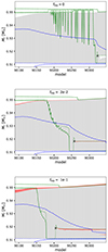 |
Fig. 1. Kippenhahn diagrams showing the PIE in a 1 M⊙, [Fe/H] = −2.5 AGB model for three different values of the overshoot coefficient at the top of the convective pulse (ftop). Convective regions are shaded gray. The dotted green and blue lines trace the mass coordinate where the nuclear energy production by hydrogen and helium burning is maximum, respectively. The dashed green and blue lines delineate the hydrogen and helium-burning zones (where the nuclear energy production by H and He burning exceeds 10 erg g−1 s−1). The red areas show the extent of the overshoot zones. The black crosses indicates where and when the convective pulse splits. |
Increasing ftop reduces the chemical discontinuity between the convective pulse and the intershell radiative zone. As a consequence, the spikes seen in the nuclear energy production (Fig. 1) are removed and the profile of Nn, max (Fig. 2) becomes smoother. The PIE also starts earlier because the growing convective pulse reaches the H-rich layers earlier (this is visible in Fig. 2, where the Nn profiles starts to rise earlier with increasing ftop). In addition, the duration of the PIE1 is shortened with increasing ftop. Indeed, for high ftop values, the PIE starts when the top of the pulse grows fast in mass; in this case, the H-rich layers that will bring the large amount of protons responsible for the pulse to split are quickly reached. In contrast, for lower ftop values, the PIE starts later, when the pulse grows more slowly, so that it takes more time to engulf the critical amount of H needed for the splitting the convective pulse.
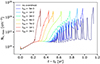 |
Fig. 2. Evolution of maximal neutron density during a PIE. The different lines correspond to different values of the overshoot coefficient at the top of the convective pulse (ftop). The evolution is illustrated between the time t0 at which Nn, max rises above 1010 cm−3 and ends when the convective pulse splits. |
Shorter PIEs translate into smaller neutron exposures2 and a higher production of elements in the Zr region, as illustrated in Fig. 3. With smaller neutron exposures the production of 36 ≤ Z ≤ 56 elements increases to the detriment of elements with Z ≥ 82 and, in particular, of the actinides (Fig. 4a). As discussed in Choplin et al. (2022b), a neutron density of at least ∼1.5 × 1015 cm−3 is required to synthesize actinides. In the 1 M⊙ model, this threshold value is obtained for low ftop ∼ 0.02.
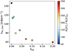 |
Fig. 3. Neutron exposure at the bottom of the convective pulse (where the neutron density, Nn, is maximum) as a function of the ftop parameter. The color indicates the Zr (Z = 40) production factor, namely, its surface abundance normalized to its initial abundance. |
3.3. The impact of overshooting at other convective boundaries
As a next step, we considered overshoot only at the bottom of the convective pulse, varying fbot from 0.02 to 0.1. As seen in Fig. 4b, setting fbot ≠ 0 produces small changes in the surface abundances by at most 0.5 dex. The elemental distribution is almost unaffected by changes in fbot as long as it is non-zero. Finally, we include overshoot only at the bottom of the convective envelope and varied fenv between 0.02 and 0.2. Here, again the impact on the surface abundances is very small (< 0.1 dex, Fig. 4c). In the end, the abundances are mostly sensitive to ftop since this parameter directly controls how protons are engulfed in the convective pulse.
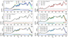 |
Fig. 4. Impact of different overshoot parameters on the surface [X/Fe] ratios after a PIE in a 1 M⊙, [Fe/H] = −2.5 AGB model. Shown are the effect of including overshooting at the top of the convective pulse (panel a), at the bottom of the convective pulse (panel b), at the bottom of the convective envelope (panel c), when varying the parameters p (with ftop = 0.02 and ftop = 0.04, panel d), and Dmin with ftop = 0.02 (panel e), and ftop = 0.04 (panel f). The bottom subplots report the difference between a given model and the first model in the list. |
3.4. The impact of the p and Dmin parameters
Finally, we investigate how the other two free parameters, p and Dmin, which control the profile of the diffusion coefficient (Eq. (2)), impact surface abundances. In a first step, p was set to 0.2, 1 or 5, with ftop = 0.02 or 0.04 and Dmin = 1 (6 models). In a second step, Dmin was varied from 10−2 to 108 cm2 s−1, with ftop = 0.02 or 0.04 and p = 1 (12 models). In both sets of models, the abundance scatter is on the order of 0.5 dex at maximum for elements with 35 < Z < 55 and for Pb and Bi (Fig. 4, panels d, e, and f). Furthermore, Th and U show greater variations and a strong dependence with p (∼1.5 − 2 dex at maximum).
3.5. Summary
Varying the overshoot parameters in our 1 M⊙ [Fe/H] = −2.5 model produces variations in the abundances of 36 < Z < 56 elements of 0.5 − 1 dex. The scatter is 2 − 3 dex for Th and U. The other elements are affected by less than 0.5 dex. Nuclei with 56 < Z < 80 have a higher predictive power because they are weakly affected by the changes in the overshoot parameters (Fig. 4). Although the nucleosynthesis may be affected, variations in the overshoot parameters have a weak impact of the structure of the PIE (provided it is present without overshooting).
4. AGB models at different masses and metallicities with overshoot
We computed models of 1, 2, 3, and 4 M⊙ with metallicities in the range of −2 < [Fe/H] ≤ 0 (Table 3). For each model, we considered four overshoot cases: no overshoot and overshoot above the pulse with ftop = 0.02, ftop = 0.04, and ftop = 0.1. These values scan the range of ftop used thus far in the literature (0.014 < ftop < 0.1, cf. Table 1). We set fenv = 0, fbot = 0, Dmin = 1 cm−3 and p = 1. The models are labeled as MX.XzY.Y_fZZ, where X.X corresponds to the mass in M⊙, Y.Y = −[Fe/H] and ZZ is the value of ftop. For instance, M1.0z2.0_f04 refers to the 1 M⊙ model at [Fe/H] = −2.0 computed with ftop = 0.04. When possible, the models were computed until the end of the TP-AGB phase. Some models were stopped before the end (cf. Table 2 for more details).
Initial mass (Mini), [Fe/H] ratio and metallicity Z of our grid models.
4.1. Evolution and nucleosynthesis of the 1 M⊙ models
Overshoot at the top of the convective pulses facilitates the development of a PIE. The higher ftop, the easier for a PIE to develop. Setting ftop = 0.02 triggers a PIE in the 1 M⊙ [Fe/H] = −2 model only (Table 2). With ftop = 0.04, a PIE develops in the [Fe/H] = −2 and −1.5 models. Finally, ftop = 0.1 gives a PIE in all 1 M⊙ models, except at solar metallicity.
In all the 1 M⊙ model where a PIE develops, a large amount of carbon (and heavy elements) is dredged-up to the surface, considerably increasing the opacity of the envelope. This boosts the mass-loss rate leading to the ejection of the entire envelope before another thermal pulse appears (cf. Sect. 3.1.4 in Choplin et al. 2021, for more details). In all our 1 M⊙ models, the AGB phase quickly ends after a PIE.
Figure 5 shows the final surface mass fractions of the 1 M⊙ models with ftop = 0.1 that experience a PIE. Generally speaking, the lower the metallicity, the heavier the elements synthesized. The main reason is that the abundance of 56Fe which acts as the main seed, increases with metallicity, so that the neutron to seed ratio decreases with increasing metallicity. More 56Fe favors the production of lighter i-process elements to the detriment of the heavier ones. A similar metallicity dependence on the distribution of heavy elements is found for the standard s-process nucleosynthesis (Gallino et al. 1998; Goriely & Mowlavi 2000; Goriely & Siess 2018). More specifically, at a metallicity of [Fe/H] = −0.5 (−1.0), only elements with 26 ≲ Z ≲ 40 (26 ≲ Z ≲ 55) are synthesized (Fig. 5). In contrast, at [Fe/H] = −1.5 (blue pattern, in Fig. 5), nuclei with Z ≳ 55 start to be significantly produced. Going down to [Fe/H] = −2.0 (orange pattern) leads to a large production of heavy elements (especially Pb and Bi) to the detriment of lighter elements. No significant Th and U are synthesized in these models because of the high ftop value (cf. Sect. 3). The final surface [X/Fe] ratios are displayed in the top panel of Fig. 6. The [Fe/H] = −1.5 and −2.0 models show a strong i-process signature with large overproduction factors up to 4 − 5 dex. As discussed previously, increasing the metallicity leads to smaller heavy elements [X/Fe] ratios.
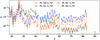 |
Fig. 5. Final surface mass fractions (after decays) for the 1 M⊙ that experiences a PIE. The different colors correspond to the metallicities −0.5 (red), −1 (green), −1.5 (blue) and −2 (orange). Models were computed with ftop = 0.1. |
4.2. Evolution and nucleosynthesis of the 2 M⊙ models
The 2 M⊙ models experiencing a PIE show a more complex evolution and nucleosynthesis than the 1 M⊙ models: after a PIE, the AGB phase resumes with the occurrence of additional thermal pulses because of the more massive envelope (typically four to five times that of the 1 M⊙ models). Also, the metals synthesized during the PIE are more diluted in the more massive envelope. As a consequence, the opacity does not rise as much as it does in the 1 M⊙ models and the mass loss is weaker, thus allowing for a “normal” thermally pulsing AGB phase.
4.2.1. A mix of s- and i-processes at [Fe/H] = −1.0
Our discussion focuses on the evolution of the 2 M⊙ model at [Fe/H] = −1.0 with ftop = 0.1, which experiences a series of more or less intense PIEs during the first six pulses and a mix of i- and s-processes. The other 2 M⊙ models with ftop = 0, 0.02 or 0.04 do not experience any PIE. Figure 7 shows the internal structure of this model during the first and second pulses. A PIE starts at model ∼25 600, associated with a maximal neutron density of Nn, max = 1.1 × 1014 cm−3 at model ∼26 000 (Fig. 7, lower panel). Shortly after the neutron peak, the pulse splits, which ends the i-process enrichment of the upper part of the pulse (cf. Sect. 3.5 in Paper III). At this point, both parts of the pulse are enriched in i-process products, especially in the first peak elements such as Sr, as can be seen by comparing panels a and b of Fig. 8. Heavier elements such as Ba and Pb are not significantly produced because of the high metallicity ([Fe/H] = −1, cf. discussion in Sect. 4.1). At model ∼26 400, the pulse merges with the convective envelope (Fig. 7) producing the elemental distribution shown in the red pattern of Fig. 9. It is important to note that after the merging, hydrogen is dredged down to Mr ∼ 0.53 M⊙, producing a significant reduction of the He core mass. As a consequence, the second pulse develops at almost the same mass coordinate as the first one (around ∼0.5321 M⊙).
After the split, a radiative zone extending between Mr ∼ 0.5312 M⊙ and 0.5323 M⊙ (Fig. 7) with a 13C/14N > 1 (Fig. 8c) forms. This “13C-pocket” (e.g., Iben & Renzini 1982) emerges naturally after the PIE in our models. As explored in various works (e.g., Straniero et al. 1995; Goriely & Mowlavi 2000; Busso et al. 2001; Bisterzo et al. 2010), it leads to a radiative s-process nucleosynthesis during the interpulse period, which lasts ∼5 × 10⁵ yr in our model. The temperature of the 13C-pocket reaches 100 MK and the neutron density goes up to 2.3 × 106 cm−3. At the end of this interpulse phase, the abundances of 138Ba and 208Pb have increased by 3 − 4 dex (Fig. 8d). These products are then engulfed in the second thermal pulse (Fig. 8e) which experiences a weaker PIE (Fig. 7). The neutron density at the bottom of the pulse goes up to 4.5 × 1012 cm−3 (it stays above 1012 cm−3 for ∼0.5 yr) and barely affects the distribution of heavy elements in the pulse, as can be seen by comparing panels e and f of Fig. 8. This second thermal pulse is followed by a third dredge up (Fig. 7) that enriches the surface in s-process products. The net result is an increase of the elements with 55 < Z < 83 by typically ∼1 dex (Fig. 9, blue pattern). The surface chemical composition is not significantly affected by the subsequent evolution. Seven more TPs develop, followed in four cases by very shallow DUPs. In the absence of overshooting below the envelope, there is no more radiative s-process episode. Weak PIEs with maximal neutron densities of 2 − 5 × 1011 cm−3 develop during the following pulses but they do not impact the surface abundances. The final surface [X/Fe] ratios are shown in the middle panel of Fig. 6 (green distribution).
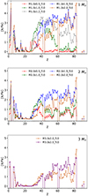 |
Fig. 6. Final surface [X/Fe] ratios for the models that experience a PIE. The different panels correspond to different initial stellar masses. The various colors correspond to different metallicities [Fe/H] −0.5 (red), −1 (green), −1.2 (grey), −1.5 (blue), −2 (dark orange), and −2.5 (purple). All these models were computed with ftop = 0.1 A few models are not shown for clarity. |
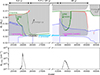 |
Fig. 7. Kippenhahn diagram showing the early AGB phase (first and second thermal pulses) of a 2 M⊙, [Fe/H] = −1.0 star (M2.0z1.0_f10 model). Convective regions are shaded gray. The dashed green and blue lines delineate the hydrogen and helium-burning zones, respectively (where the nuclear energy production by H and He burning exceeds 10 erg g−1 s−1). The red area shows the extent of overshooting. The magenta (cyan) line indicates the region zones where the i-process (s-process) nucleosynthesis occurs. The bottom panel shows the maximal neutron density as a function of the model number, or equivalently time as indicated in the upper x-axis. |
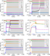 |
Fig. 8. Abundance profiles of the M2.0z1.0_f10 model before the PIE (model 25344, panel a); right after the PIE (model 26044, panel b); just after the merging between the pulse and envelope (model 26544, panel c); at the end of the interpulse (model 42644, panel d); at the very start of the second thermal pulse (model 43586, panel e); and after the second weak PIE (model 44597, panel f). |
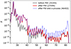 |
Fig. 9. Elemental mass fractions at the surface of the M2.0z1.0_f10 model at three different times. The numbers in parenthesis correspond to the model number of Fig. 7. |
4.2.2. Case of a 2 M⊙ model at [Fe/H] = −1.5
The evolution of the 2 M⊙ model at [Fe/H] = −1.5 with ftop = 0.1 resembles that of the 2 M⊙ model at [Fe/H] = −1.0. A PIE develops during the first pulse, followed by a radiative s-process episode (with neutron densities of 5 × 106 cm−3 at maximum). The s-process products are engulfed in the second pulse, in which a weak PIE takes place. The second pulse is then followed by a third dredge up. After that, this model experiences five more pulses with weak PIEs (and three DUPs) before it has completely lost its envelope.
The resulting nucleosynthesis is however very different compared to the [Fe/H] = −1.0 model (green and blue patterns in Fig. 6, middle panel). As explained in Sect. 4.1, the reduced iron content in the [Fe/H] = −1.5 model allows for a stronger i-process and favors the synthesis of heavier elements. The neutron density peak is higher in the [Fe/H] = −1.5 model (4.7 × 1014 cm−3) compared to the [Fe/H] = −1.0 model (1.1 × 1014 cm−3) resulting in a stronger heavy nuclei production which masks the s-process contribution in the region of 55 < Z < 83 (cf. the red and green patterns in Fig. 10). Ultimately, the chemical yields of this model are mostly determined by the first PIE. Only elements with 30 ≲ Z ≲ 40 are altered (typically 1 dex) by the nucleosynthesis (radiative s-process and weak PIEs) following the first PIE (Fig. 10).
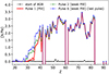 |
Fig. 10. Surface [X/Fe] ratios in the M2.0z1.5_f10 model at four different times. Abundances are shown after the dredge up following the indicated pulse number (except for the black pattern that corresponds to the start of the AGB phase). |
4.2.3. Other 2 M⊙ models
The M2.0z0.5_f10 model follows a very similar evolution as the M2.0z1.0_f10 model (cf. Sect. 4.2.1), namely: a weak PIE followed by a radiative s-process which is mixed in the following pulse and eventually dredged up to the surface. In Karinkuzhi et al. (2023), a 2 M⊙ model at [Fe/H] = −0.5, with ftop = 0.06, fenv = 0.06, Dmin = 107 cm−3 and p = 0.5 was computed to explain the two newly observed r/s-stars at [Fe/H] = −0.5. This model experienced a PIE during the third thermal pulse, resulting in a rather strong i-process signature. The 2 M⊙, [Fe/H] = −0.5 model with ftop = 0.1 computed in this work also experiences a PIE but during the second pulse instead (Table 2) and shows a mixed i + s signature (red pattern in middle panel of Fig. 6). The differences in the mixing parameters are likely at the origin of the different chemical patterns. As a matter of fact, the i-process (and potentially s-process) yields remains very sensitive to the overshoot parameters.
A PIE develops in the M2.0z2.0_f04 and M2.0z2.0_f10 models during the second and first pulse respectively. The final surface abundances in these two models differ by ∼0.5 − 1 dex but follows the same trend. In particular, heavy elements such as Pb and Bi are heavily produced (Fig. 6). In the M2.0z2.0_f10 model, after the first PIE, the elements with 30 ≲ Z ≲ 50 are slightly enhanced because of the additional weak PIEs and third dredge ups (cf. Sect. 4.2.2).
The yields of 1 and 2 M⊙ models have the same metallicity dependence with a smaller production of heavier elements with increasing metal content. However, because of its larger mass, the enrichment of PIE products in the 2 M⊙ models is lower. Also, the s-process signature present in the M2.0z1.0 and M2.0z0.5 models and characterized by the production of elements between Z ∼ 55 and Z = 83 is absent in the lower mass models because of their truncated evolution.
4.3. Evolution and nucleosynthesis of the 3 and 4 M⊙ models
The 3 M⊙ model at [Fe/H] = −2 experiences a PIE during the second pulse for ftop = 0.1 followed by five pulses during which weak PIEs develop (like in Fig. 7) with Nn, max = 2.7 × 1012 cm−3 at maximum. These weak PIEs are sometimes followed by a third dredge up but this barely changes the surface abundances, which are largely determined by the first strong PIE. A radiative s-process develops after the PIE of this model but is too weak to significantly alter the i-process signature.
A PIE also develops in the 3 M⊙ model at [Fe/H] = −2.5, both with ftop = 0.04 and 0.10. The PIE develops during the third (second) pulse for ftop = 0.04 (0.10). The pulse conditions are different between the second and third pulses. In particular, the maximal temperatures at the bottom of the pulse reach 281 and 266 MK for the ftop = 0.04 and 0.10 cases, respectively. Also, the energy released during these two events are different, which imply different amount of ingested proton. This impacts the i-process nucleosynthesis and surface abundances (Fig. 11). Like the 3 M⊙ model at [Fe/H] = −2, weak PIEs develop during the next pulses, altering the surface [X/Fe] ratios of elements with 31 < Z < 41 by about 0.3 dex at maximum. Here again, the radiative s-process is too weak to significantly alter the i-process signature.
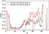 |
Fig. 11. Final elemental [X/Fe] ratios at the surface of the M3.0z2.5_f04 and M3.0z2.5_f10 models. |
The global level of enrichment for the 3 M⊙ is smaller than for the 1 and 2 M⊙ models since the PIE products are diluted in a larger envelope: at [Fe/H] = −2, the 1, 2 and 3 M⊙ models have convective envelopes of 0.24, 1.18, and 1.83 M⊙, respectively, at the time of the PIE. Also, the pulse mass decreases with increasing mass (0.049, 0.027, and 0.009 M⊙ for the 1, 2 and 3 M⊙ models, respectively). To summarize: with increasing stellar masses, the i-process material is diluted in more massive envelopes, resulting in lower level of enrichment but the chemical patterns remain similar (Fig. 6).
The 4 M⊙ model at [Fe/H] = −2 does not experience any PIE during the 28 thermal pulses computed, even when adopting ftop = 0.1 (Table 2). At this stage, only ∼0.3 M⊙ of envelope is left. We also confirmed that for high enough ftop values (typically 0.2), a PIE develops during the early AGB phase of this model.
4.4. Mass and metallicity range of PIEs
We previously showed that without overshoot, PIEs develop in AGB models having an initial mass below about 2.5 M⊙ and a metallicity, Z, below about 10−4 in mass fraction (Paper III). This defines a minimal PIE region (or i-process zone), which is represented by the shaded grey area in Fig. 12. The thick black boundary in Fig. 12 is obtained by a classifier using a Gaussian radial basis function kernel and trained on both the models from this work and from literature to separate models undergoing PIEs to other models.
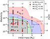 |
Fig. 12. Mass-metallicity diagram showing the occurrence of PIEs during the early AGB phase. The corresponding [Fe/H] ratios are indicated on the right axis assuming solar-scaled mixtures. Red filled circles show AGB models experiencing a PIE when ftop = 0. Empty black circles are for models that do not experience a PIE when ftop = 0. Thick black circles denotes models computed in this work and in Paper III. The small red circles and red dots highlight our models that experience a PIE when ftop = 0.04 and 0.10, respectively. The other models are from Iwamoto et al. (2004), Campbell & Lattanzio (2008), Cristallo et al. (2009a, 2016), Lau et al. (2009), Suda & Fujimoto (2010). The four colored zones show the approximate PIE zone when ftop = 0, 0.02, 0.04 and 0.10. |
The models computed in this work with different overshoot strengths at the top of the convective pulse (ftop) provide a first estimate of the extent of the PIE zone as a function of ftop (Fig. 12). As expected, the higher ftop, the more extended this zone. For high enough ftop, PIEs can develop close to solar-metallicity. However, it seems that PIE could hardly take place in AGB stars with initial masses higher than 4 M⊙ (unless the metallicity is very low or ftop very high).
Knowing the location of this PIE boundary is important to assess the contribution of AGB stars to the i-process nucleosynthesis. This boundary remains extremely sensitive to the modeling of overshooting and, in particular, to the adopted value of the ftop parameter. Hydrodynamical simulations have shown that convection extends beyond the boundary of the convectively unstable region but presently, to our knowledge, there is no clear constraint on the ftop value. In particular, we cannot rule out high ftop values of ftop = 0.1, for instance. The ftop values used so far in the literature range between 0.014 and 0.1 (Table 1). For fenv, values higher than 0.1 were sometimes used to obtain a massive enough 13C-pocket to account for the surface s-process enrichment in AGB stars (e.g., Pignatari et al. 2016; Ritter et al. 2018).
5. Comparison with observations
In Choplin et al. (2021, 2022c), we have shown that the i-process nucleosynthesis in a 1 M⊙ AGB model at [Fe/H] = −2.5 was compatible with 14 observed r/s-stars with −2.70 < [Fe/H] < −2.26. Here, we examine whether such a comparison remains true when considering higher metallicity stars. We first searched for some r/s-stars candidates with −2 < [Fe/H] < −1 and investigated whether our AGB models with overshoot can account for their chemical abundance patterns.
5.1. r/s-stars sample
To search for r/s-stars candidates, we used the dRMS proxy introduced in Karinkuzhi et al. (2021) to classify s-, r-, and r/s-stars. It is defined as
 (3)
(3)
with N as the number of considered heavy elements and Ai, ⋆ = log10(ni, ⋆/nH, ⋆)+12, where ni, ⋆ is the number density of element i in the sample star. The quantity Ai, r corresponds to the solar r-process abundance of element i scaled to the Eu abundance of the sample star. It is computed as
 (4)
(4)
where Ai, r, ⊙ is the solar r-process abundance of element i from Arnould et al. (2007). The s-, r-, and r/s-stars have been shown to be rather well identified when using this criterion (Fig. 10 of Karinkuzhi et al. 2021). The r/s-stars are characterized by intermediate dRMS values, typically between 0.5 and 1. For our study, we selected potential i-process stars candidates from the SAGA database (Suda et al. 2008, 2017). We complemented these data with a few recent observations (see Table 4 for more details) using the following filters: (1) a metallicity in the range −2 < [Fe/H] < −1, (2) an enrichment in barium relative to iron [Ba/Fe] > 0.5, (3) at least five measured abundances between Ga (Z = 31) and Pb (Z = 82), and (4) a heavy-element pattern characterized by 0.4 < dRMS < 1. This gives us a sample of 22 stars: 8 dwarfs or Main Sequence (MS), 10 red giants (RG), and 4 post-AGB stars, as summarized in Table 4.
Characteristics of the 22 selected stars.
5.2. Different scenarios for MS and RG stars and post-AGB stars
For MS and RG stars, the enrichment in trans-iron elements could come from a now-extinct AGB companion that polluted the secondary through winds (e.g., Abate et al. 2013). This scenario predicts that r/s-stars ought to reside in binary systems. This was indeed shown in most cases (e.g., 9 out of 11 r/s-stars in Karinkuzhi et al. 2021, are confirmed binaries). In our sample however, only 6 MS/RG stars out of 18 were clearly identified as binaries (Table 4), while the 9 other stars are either single, long-period binary systems or binary systems with a high orbital axis inclination, which hinders the detection of radial velocity variations. The binarity of the remaining three RG stars was not investigated, to our knowledge. Radial velocity monitoring over long periods of time is desired to unveil the binary status of these stars. An alternative scenario that does not require binarity is to rely on an early generation of AGB stars that polluted with i-process material the natal cloud of these stars.
The four post-AGB stars in our sample may be intrinsically enriched, having synthesized heavy element in their interior. In this case, there is no need to account for an AGB companion as it would be for MS and RG stars. The surface composition can be directly compared to our AGB model predictions. To do so, we assumed that the final surface abundances of our AGB models are not further affected by the late AGB and post-AGB evolution and, therefore, they do reflect the post-AGB abundances. Although most of our models have reached the end of the AGB phase (Table 2), they may still experience a late pulse, possibly altering their final surface abundances (Herwig et al. 2011; De Smedt et al. 2012). Computing the post-AGB phase of these models is beyond the scope of this work, but this would be required to strengthen our comparisons with observations.
5.3. Fitting procedure
We followed the same procedure as in Sect. 6.2 of Choplin et al. (2021) to find the lowest χ2 among our AGB models. In particular, we used  , which represents the χ2 normalized by the number of data points (i.e., by the number of derived elemental abundances). When the AGB material is diluted in the unpolluted envelope of the MS or RG companion (Xini), the resulting mass fraction of an isotope i is given by:
 (5)
(5)
where 0 ≤ fdil < 1 is the dilution factor, while Xs and Xini are the surface and initial mass fractions of isotope i, respectively. For post-AGB stars, we have fdil = 0.
To compute the  value, we consider the abundance of elements heavier than Zn (Z = 30). Nuclei from Na (Z = 11) to Zn (Z = 30) are scarcely impacted by low-mass AGB nucleosynthesis and their presence in the stellar envelope may originate from previous sources that polluted the proto-stellar gas (e.g., winds and/or core-collapse supernovae of massive stars). The C, N, and O abundances are more difficult to interpret as these elements are impacted by the AGB donor nucleosynthesis, could be present in non-solar proportions in the proto-stellar cloud or be altered by internal mixing processes in the observed star when it evolved, for example, into a giant. These elements are discussed in the next sections, but they are not considered in the determination of the minimal
  .
.
For each of the 22 observed stars, we selected the three best AGB models for which the metallicity is within 0.5 dex of the observed value (e.g., only our models with [Fe/H] = −1.5 and −2.0 are considered to describe the abundances of BS 16080−175, which has a metallicity of [Fe/H] = −1.86).
5.4. Heavy elements
5.4.1. MS and RG stars
A reasonable agreement between models and observations was found for the 18 MS and RG stars (Figs. 13, 14, and A.1), with residuals less than ±0.5 dex (Fig. 13) in most cases. This is reasonable in view of the various uncertainties associated with observations (typically 0.2 − 0.5 dex), numerics (±0.3 dex on the abundances Choplin et al. 2021), nuclear physics (e.g., Goriely et al. 2021; Martinet et al. 2024; Choplin et al. 2022a), and mixing processes, such as the overshoot description discussed in Sect. 3.
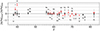 |
Fig. 13. Residual of the best fits for the 16 i-process stars candidates of Table 4. Black points correspond to MS and RG stars, while red points are for post-AGB stars. The crosses represent the average values of the residuals. The individual fits are shown in Figs. 14 and A.1. |
As shown in Fig. 15, the different abundance ratios can be reasonably well accounted for by our models. Two stars (HD 209621 and HE 1120−2122) have [La/Eu] ≃ 0 and [La/Y] ≃ 1, which is ≃0.5 dex away from the closest model track. These stars have a particularly low [Y/Fe] (about 0.5, Fig. A.1) but high abundances of Sr and Zr which are nearby elements. This scatter cannot be reproduced by our models, which predict minimal  values of 4.32 and 2.19 (Table 4, these values drop to 2.46 and 1.25 when excluding Sr, Y and Zr from the adjustment). One RG star (T6953-00510-1) has [La/Eu] = 0.93, which is at the limit of our model predictions (∼0.8) and exhibits a value of a dRMS = 0.97 (Table 4), which may point towards an s-process (rather than i-process) as its origin. Although the negative [Ba/La] ratio of several stars is not compatible with our model predictions (Fig. 15, bottom panel), Martinet et al. (2024) showed, based on a 1 M⊙ AGB model with [Fe/H] = −2.5, that nuclear uncertainties introduce a spread in the [Ba/La] ratio of −0.75 < [Ba/La] < 0.63 (their Sect. 3.3.1). As a test, we re-computed the PIE in the M2.0z2.0_f10 model using a different set of (n, γ) rates and found that a final surface [Ba/La] ratio lower by about 0.4 dex, giving a dilution curve relatively consistent with observations with [Ba/La] < 0. It remains to be checked if the observational scatter in Fig. 15 can be covered when this alternative set of nuclear rates is adopted for all our stellar models. This task goes beyond the scope of the present paper but would be required to draw solid conclusions.
5.4.2. Post-AGB stars
For post-AGB stars, there is no adjusting dilution factor and good-quality fits are more difficult to obtain. Nevertheless, the post-AGB star J004441 can be well explained by our M1.8z1.5_f10 AGB model (Fig. 14, bottom panel). This agreement is also acceptable for the three other post-AGB stars except for Y and Zr, which are overestimated in our calculations (Figs. 13 and A.1). For these objects,  ∼ 5 − 6 but if we exclude Y and Zr from the fit, it drops to 0.5 − 1.7 (Table 4). As for the RG star T6953-00510-1, the [La/Eu] ratio of post-AGB stars is hard to reconcile with our predictions. The post-AGB J051848 has the highest value of [La/Eu] = 1.16 which is ∼0.4 dex above our model values (Fig. 15), but compatible with nuclear uncertainties. The rather high [La/Eu] ratios together with the dRMS of 0.8 − 1 (Table 4) indicate that these objects have an unclear chemical signature between the s- and the i-process.
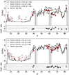 |
Fig. 14. Best description of the RG star HE 2144−1832 (top panel) and post-AGB star J004441 (bottom panel) using the AGB models computed in this work (Table 2). The three best models are shown in black (lowest |


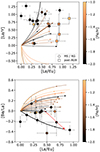 |
Fig. 15. [La/Y] and [Ba/La] abundance ratios as a function of [La/Eu]. Circles correspond to MS and RG stars while squares are for post-AGB stars. Lines represent the dilution curves of the AGB material, which ultimately produce a material of solar composition (i.e., ratios equal to zero). Lines and symbols are color-coded according to the metallicity [Fe/H]. The small squares on the lines indicates where fdil = 0.9. The thick black line (bottom panel) shows a 2 M⊙, [Fe/H] = −2 model computed with a different set of neutron capture rates (see text for more details) and the red arrow shows the resulting abundance displacement. |
5.5. The C, N, O elements
The [C/Fe] ratios can be relatively well accounted for (Figs. 14 and A.1), even if they were not included in the  fitting procedure. The exception is CS 22880−074 with [C/Fe] = 1.42 while our best models predict [C/Fe] ≤ 0.5. Three other stars (BS 160080−175, BS 17436−058 and HD 5223) have a [C/Fe] ratio ≃0.5 dex above our model predictions. The agreement for [N/Fe] is acceptable for several stars. However, for five stars – BS 17436−058, HD 206983, HD 209621, HE 1120−2122, and T6953-00510-1 – [N/Fe] is ∼1 dex above our model predictions (∼2 dex for T6953-00510-1). Finally, the high [O/Fe] of ≃1 of several MS and RG stars – HD 126681, HD 166161, HD 166913, HD 209621, HE 1120−2122 and T6953-00510-1 – cannot be accounted for by our models. The four post-AGB stars have also [O/Fe] ≃ 1, but our models predict [O/Fe] ≃ 0.5 at maximum.
In summary, for the stars mentioned above, C, N, and O are always underproduced by our models, which may suggest an early CNO enrichment by external sources such as massive stars. Some of the discrepancies for [C/Fe] and [O/Fe] can be attributed to the fact that we did not consider α-enrichment in our initial composition. In particular, with [O/Fe] ratios increased by 0.4−0.7 dex for metallicities below [Fe/H] < −1 (Bensby et al. 2014), the agreement would be significantly improved. Nevertheless, using a different initial mixture may potentially impact the PIEs because the metallicity (Z) is affected, thereby preventing us from drawing firm conclusions without computing additional models. The high N abundances might originate from previous rotating massive stars that are known to overproduce N, especially at low metallicities (e.g., Meynet et al. 2006).
5.6. Accretion and dilution for MS and RG stars
Although the binary status is not confirmed for a significant fraction of the sample stars (Sect. 5.2 and Table 4), we can still estimate how much mass the r/s-stars should have accreted from their AGB companion, if they were all indeed binary. As developed in Choplin et al. (2021, 2022c), in the binary mass transfer scenario, the dilution factor fdil (Eq. (5)) can be linked to the envelope mass of the r/s-star before the accretion episode (Menv) and the mass accreted by the r/s-star (Macc) as:
 (6)
(6)
For a low-metallicity 1 M⊙ star, the envelope mass on the main sequence is on the order of Menv = 5 × 10⁻⁴ M⊙ and around Menv = 0.4 M⊙ on the giant branch. Using these values, we find (Table 4) 2.0 × 10⁻⁶ < Macc/M⊙ < 0.16, with 11 out of 18 stars having Macc < 10−2 M⊙ and 9 out of 18 star with Macc < 10−3 M⊙. The star with the highest Macc of 0.16 M⊙ is J130200.0−084328. Its best fit is obtained by our 3 M⊙ AGB model at [Fe/H] = −2.0 (Fig. A.1). Considering that more than 2 M⊙ will be lost by the AGB phase of this model, it does not seem unrealistic to assume that the secondary could accrete 0.16 M⊙ (i.e., ∼8%) of that wind material. Although simple, this estimate confirms that the accretion scenario for these r/s-stars is not unrealistic. However, as discussed in Sect. 5.3, the binary status of our sample stars remains unclear and will need to be elucidated.
5.7. Comparison with previous studies: r + s scenario
Eight of our sample stars, BS 16080−175, BS 17436−058, CS 22880−074, CS 22887−048, CS 29513−032, HD 206983, HD 209621, and HD 5223, were analyzed by Bisterzo et al. (2012). They used AGB models computed by Bisterzo et al. (2010), which experience an s-process nucleosynthesis through the artificial introduction of a 13C-pocket with varying efficiencies. In seven out of these eight stars, they considered an r + s scenario: they mixed a variable fraction of solar r-process material to the s-process material of their AGB models to fit the observed abundances. The abundances of these stars are reasonably well reproduced in the framework of the r + s scenario, except for Y and W in HD 209621 (overproduced and underproduced by 1 − 1.5 dex in the model) and Y in HD 5223 (overproduced by 0.5 − 1 dex). We faced rather similar issues for these stars, although the agreement with W in HD 209621 is relatively better (underproduced in our models by 0.7 dex, Fig. A.1). These authors did not consider an r-process contribution for the eighth star (CS 22880−074), but its abundances are reasonably well reproduced by an s-process operating in the 1.3 M⊙ AGB model (except for Er which is underestimated by 0.5 dex). The observed abundances of the post-AGB star J004441 were also shown to be well reproduced in the framework of the r + s scenario (Cui et al. 2014). At this stage, there is no clear preference between the i and r + s scenario for these stars. A dedicated study would be required to determine whether certain key observations (especially elemental or isotopic ratios) could help in distinguishing between the i- versus the r + s scenarios.
6. Summary and conclusions
In this work, we studied the i-process developing during a PIE in AGB stellar models of various initial masses and metallicities, including the possibility to have overshoot mixing at convective boundaries. The models were computed with the code STAREVOL in which a network of 1160 nuclei is used and coupled to the transport equations.
A detailed study of the impact of all overshoot parameters was first carried out during the PIE of a 1 M⊙, [Fe/H] = −2.5 model. In particular, we considered different overshoot coefficients above and below the thermal pulse, as well as below the convective envelope. While a PIE always develops in this model star regardless of the overshoot assumptions, the final surface abundances of 36 < Z < 56 elements show an overall scatter of 0.5 − 1 dex, which goes up to 2 − 3 dex for Th and U. Because the abundances of 56 < Z < 80 elements are impacted by less than 0.5 dex by the different overshoot assumptions (at least in the considered AGB model), the predictive power of our i-process models is higher for these nuclei. Actinides are only significantly produced if the overshoot at the top of the convective pulse is low enough (ftop ≲ 0.04).
We then investigated AGB models with 1 ≤ Mini/M⊙ ≤ 4 and metallicities −2 ≤ [Fe/H] ≤ 0. In these cases, the overshoot mixing at the top of the convective thermal pulse is found to play a key role in favoring the development of a PIE. While for ftop = 0, no PIE develops, for low (0.02), medium (0.04), and high (0.10) ftop values, we found that 6%, 24%, and 86% of our AGB models, respectively, experience a PIE (Table 2). In the mass-metallicity diagram, the PIE region is extended with increasing ftop, almost reaching solar metallicity for high ftop values (Fig. 12) In the framework of our calculations, the chemical imprint of the i-process is increased with decreasing metallicity, and mainly affects heavy elements with Z > 30. We also found that PIEs leave a 13C-pocket at the bottom of the pulse that can give rise to an additional radiative s-process nucleosynthesis. The s-process products either stay locked deep into the star or are dredged-up to the surface but, in this case, remain generally overwhelmed by the higher i-process enrichment. In our 2 M⊙ models at [Fe/H] = −1.0 and −0.5, this 13C-pocket leads to a noticeable mixed signature of i + s elements at the AGB surface. After the first main PIE, our models with Mini > 1 M⊙ experience weak PIEs that further impact the surface abundances of 31 < Z < 41 elements.
Finally, based on the classification scheme of r/s-stars introduced by Karinkuzhi et al. (2021), a sample of 22 observed main sequence, giant, and post-AGB stars with −2 < [Fe/H] < −1 was selected and compared to our models. The [X/Fe] ratios of nuclei with Z > 30 can be reasonably well reproduced by our models, with residuals generally restricted to the range of ±0.5 dex, with a clear exception for Y and Zr in three post-AGB stars. The overall good agreement found between r/s-stars candidates and our AGB models at −2 < [Fe/H] < −1 is in favour of an i-process operating in AGB stars up to [Fe/H] ≃ −1 at least. Radial velocity monitoring over long periods of time is desired to unveil the binary status of these r/s-stars. If these stars are in binary systems, our simple estimate for the mass that should be accreted from the AGB companion to explain the level of i-process enrichment leads to realistic values. If these stars are single, an alternative scenario needs to be considered, for instance, by assuming they formed from an i-process enriched material left by an early generation of AGB stars. At this stage, the r + s scenario (in which two distincts sources have produced a mixed r/s abundance pattern) cannot be excluded.
The occurrence of PIEs (hence the i-process) in AGB stars remains very sensitive to the adopted overshoot parametrization, especially with respect to the ftop parameter, as shown in this work. A strong overshoot favors the occurrence of PIEs, even in solar-metallicity AGB stars. Constraints on the overshoot parameters (e.g., from multi-dimensional hydrodynamical models) could deliver new insights into the contribution of AGB stars to the heavy element nucleosynthesis, thus offering a step forward in understanding the chemical evolution of the Universe.
The duration of the PIE is arbitrarily defined from the time the maximal neutron density first rises above 1010 cm−3 until the convective pulse splits.
The neutron exposure τ is computed as τ = ∫Nn vT dt where Nn is the neutron density and  the neutron thermal velocity with kB the Boltzmann constant, T the temperature fixed to 250 MK, and mn the neutron mass.
Acknowledgments
This work was supported by the Fonds de la Recherche Scientifique-FNRS under Grant No. IISN 4.4502.19. L.S. and S.G. are senior F.R.S.-FNRS research associates. A.C. is post-doctorate F.R.S.-FNRS fellow.
References
- Abate, C., Pols, O. R., Izzard, R. G., Mohamed, S. S., & de Mink, S. E. 2013, A&A, 552, A26 [NASA ADS] [CrossRef] [EDP Sciences] [Google Scholar]
- Allen, D. M., Ryan, S. G., Rossi, S., Beers, T. C., & Tsangarides, S. A. 2012, A&A, 548, A34 [NASA ADS] [CrossRef] [EDP Sciences] [Google Scholar]
- Aoki, W., Ryan, S. G., Norris, J. E., et al. 2002a, ApJ, 580, 1149 [Google Scholar]
- Aoki, W., Norris, J. E., Ryan, S. G., Beers, T. C., & Ando, H. 2002b, PASJ, 54, 933 [NASA ADS] [CrossRef] [Google Scholar]
- Aoki, W., Beers, T. C., Christlieb, N., et al. 2007, ApJ, 655, 492 [NASA ADS] [CrossRef] [Google Scholar]
- Arnould, M., & Goriely, S. 2020, Progr. Part. Nucl. Phys., 112, 103766 [NASA ADS] [CrossRef] [Google Scholar]
- Arnould, M., Goriely, S., & Takahashi, K. 2007, Phys. Rep., 450, 97 [Google Scholar]
- Asplund, M., Grevesse, N., Sauval, A. J., & Scott, P. 2009, ARA&A, 47, 481 [NASA ADS] [CrossRef] [Google Scholar]
- Battino, U., Pignatari, M., Ritter, C., et al. 2016, ApJ, 827, 30 [NASA ADS] [CrossRef] [Google Scholar]
- Bensby, T., Feltzing, S., & Oey, M. S. 2014, A&A, 562, A71 [NASA ADS] [CrossRef] [EDP Sciences] [Google Scholar]
- Bihain, G., Israelian, G., Rebolo, R., Bonifacio, P., & Molaro, P. 2004, A&A, 423, 777 [NASA ADS] [CrossRef] [EDP Sciences] [Google Scholar]
- Bisterzo, S., Gallino, R., Straniero, O., Cristallo, S., & Käppeler, F. 2010, MNRAS, 404, 1529 [NASA ADS] [Google Scholar]
- Bisterzo, S., Gallino, R., Straniero, O., Cristallo, S., & Käppeler, F. 2011, MNRAS, 418, 284 [Google Scholar]
- Bisterzo, S., Gallino, R., Straniero, O., Cristallo, S., & Käppeler, F. 2012, MNRAS, 422, 849 [Google Scholar]
- Boesgaard, A. M., Rich, J. A., Levesque, E. M., & Bowler, B. P. 2011, ApJ, 743, 140 [Google Scholar]
- Burris, D. L., Pilachowski, C. A., Armandroff, T. E., et al. 2000, ApJ, 544, 302 [Google Scholar]
- Busso, M., Gallino, R., Lambert, D. L., Travaglio, C., & Smith, V. V. 2001, ApJ, 557, 802 [CrossRef] [Google Scholar]
- Caffau, E., Bonifacio, P., Faraggiana, R., et al. 2005, A&A, 441, 533 [NASA ADS] [CrossRef] [EDP Sciences] [Google Scholar]
- Campbell, S. W., & Lattanzio, J. C. 2008, A&A, 490, 769 [NASA ADS] [CrossRef] [EDP Sciences] [Google Scholar]
- Choplin, A., Hirschi, R., Meynet, G., et al. 2018, A&A, 618, A133 [NASA ADS] [CrossRef] [EDP Sciences] [Google Scholar]
- Choplin, A., Siess, L., & Goriely, S. 2021, A&A, 648, A119 [NASA ADS] [CrossRef] [EDP Sciences] [Google Scholar]
- Choplin, A., Siess, L., & Goriely, S. 2022a, A&A, 667, A155 [NASA ADS] [CrossRef] [EDP Sciences] [Google Scholar]
- Choplin, A., Goriely, S., & Siess, L. 2022b, A&A, 667, L13 [NASA ADS] [CrossRef] [EDP Sciences] [Google Scholar]
- Choplin, A., Siess, L., & Goriely, S. 2022c, A&A, 662, C3 [NASA ADS] [CrossRef] [EDP Sciences] [Google Scholar]
- Cowan, J. J., & Rose, W. K. 1977, ApJ, 212, 149 [Google Scholar]
- Cristallo, S., Piersanti, L., Straniero, O., et al. 2009a, PASA, 26, 139 [Google Scholar]
- Cristallo, S., Straniero, O., Gallino, R., et al. 2009b, ApJ, 696, 797 [NASA ADS] [CrossRef] [Google Scholar]
- Cristallo, S., Piersanti, L., Straniero, O., et al. 2011, ApJS, 197, 17 [NASA ADS] [CrossRef] [Google Scholar]
- Cristallo, S., Karinkuzhi, D., Goswami, A., Piersanti, L., & Gobrecht, D. 2016, ApJ, 833, 181 [Google Scholar]
- Cui, W., Zhang, B., & Zhao, G. 2014, Sci. China Phys. Mech. Astron., 57, 1201 [NASA ADS] [CrossRef] [Google Scholar]
- De Smedt, K., Van Winckel, H., Karakas, A. I., et al. 2012, A&A, 541, A67 [NASA ADS] [CrossRef] [EDP Sciences] [Google Scholar]
- De Smedt, K., Van Winckel, H., Kamath, D., et al. 2014, A&A, 563, L5 [NASA ADS] [CrossRef] [EDP Sciences] [Google Scholar]
- De Smedt, K., Van Winckel, H., Kamath, D., & Wood, P. R. 2015, A&A, 583, A56 [NASA ADS] [CrossRef] [EDP Sciences] [Google Scholar]
- Fabbian, D., Nissen, P. E., Asplund, M., Pettini, M., & Akerman, C. 2009, A&A, 500, 1143 [NASA ADS] [CrossRef] [EDP Sciences] [Google Scholar]
- Fishlock, C. K., Karakas, A. I., Lugaro, M., & Yong, D. 2014, ApJ, 797, 44 [Google Scholar]
- Freytag, B., Ludwig, H. G., & Steffen, M. 1996, A&A, 313, 497 [NASA ADS] [Google Scholar]
- Frischknecht, U., Hirschi, R., Pignatari, M., et al. 2016, MNRAS, 456, 1803 [Google Scholar]
- Fujiya, W., Hoppe, P., Zinner, E., Pignatari, M., & Herwig, F. 2013, ApJ, 776, L29 [Google Scholar]
- Fulbright, J. P., & Johnson, J. A. 2003, ApJ, 595, 1154 [NASA ADS] [CrossRef] [Google Scholar]
- Gallino, R., Arlandini, C., Busso, M., et al. 1998, ApJ, 497, 388 [Google Scholar]
- Gil-Pons, P., Doherty, C. L., Campbell, S. W., & Gutiérrez, J. 2022, A&A, 668, A100 [NASA ADS] [CrossRef] [EDP Sciences] [Google Scholar]
- Goriely, S., & Mowlavi, N. 2000, A&A, 362, 599 [NASA ADS] [Google Scholar]
- Goriely, S., & Siess, L. 2018, A&A, 609, A29 [NASA ADS] [CrossRef] [EDP Sciences] [Google Scholar]
- Goriely, S., Chamel, N., Janka, H. T., & Pearson, J. M. 2011a, A&A, 531, A78 [NASA ADS] [CrossRef] [EDP Sciences] [Google Scholar]
- Goriely, S., Bauswein, A., & Janka, H.-T. 2011b, ApJ, 738, L32 [Google Scholar]
- Goriely, S., Siess, L., & Choplin, A. 2021, A&A, 654, A129 [NASA ADS] [CrossRef] [EDP Sciences] [Google Scholar]
- Goswami, A., Aoki, W., Beers, T. C., et al. 2006, MNRAS, 372, 343 [Google Scholar]
- Gratton, R. G., Sneden, C., Carretta, E., & Bragaglia, A. 2000, A&A, 354, 169 [NASA ADS] [Google Scholar]
- Gratton, R. G., Carretta, E., Claudi, R., Lucatello, S., & Barbieri, M. 2003, A&A, 404, 187 [NASA ADS] [CrossRef] [EDP Sciences] [Google Scholar]
- Hansen, C. J., Primas, F., Hartman, H., et al. 2012, A&A, 545, A31 [NASA ADS] [CrossRef] [EDP Sciences] [Google Scholar]
- Hansen, T. T., Andersen, J., Nordström, B., et al. 2016, A&A, 588, A3 [NASA ADS] [CrossRef] [EDP Sciences] [Google Scholar]
- Hansen, T. T., Simon, J. D., Li, T. S., et al. 2023, A&A, 674, A180 [NASA ADS] [CrossRef] [EDP Sciences] [Google Scholar]
- Herwig, F. 2000, A&A, 360, 952 [NASA ADS] [Google Scholar]
- Herwig, F. 2005, ARA&A, 43, 435 [NASA ADS] [CrossRef] [Google Scholar]
- Herwig, F., Bloecker, T., Schoenberner, D., & El Eid, M. 1997, A&A, 324, L81 [NASA ADS] [Google Scholar]
- Herwig, F., Blöcker, T., Langer, N., & Driebe, T. 1999, A&A, 349, L5 [NASA ADS] [Google Scholar]
- Herwig, F., Freytag, B., Fuchs, T., et al. 2007, in Why Galaxies Care About AGB Stars: Their Importance as Actors and Probes, eds. F. Kerschbaum, C. Charbonnel, & R. F. Wing, ASP Conf. Ser., 378, 43 [NASA ADS] [Google Scholar]
- Herwig, F., Pignatari, M., Woodward, P. R., et al. 2011, ApJ, 727, 89 [Google Scholar]
- Iben, I., Jr., & Renzini, A. 1982, ApJ, 263, L23 [NASA ADS] [CrossRef] [Google Scholar]
- Iwamoto, N., Kajino, T., Mathews, G. J., Fujimoto, M. Y., & Aoki, W. 2004, ApJ, 602, 377 [Google Scholar]
- Jadhav, M., Pignatari, M., Herwig, F., et al. 2013, ApJ, 777, L27 [NASA ADS] [CrossRef] [Google Scholar]
- Jonsell, K., Edvardsson, B., Gustafsson, B., et al. 2005, A&A, 440, 321 [NASA ADS] [CrossRef] [EDP Sciences] [Google Scholar]
- Jorissen, A., Van Eck, S., Van Winckel, H., et al. 2016, A&A, 586, A158 [NASA ADS] [CrossRef] [EDP Sciences] [Google Scholar]
- Just, O., Bauswein, A., Ardevol Pulpillo, R., Goriely, S., & Janka, H.-T. 2015, MNRAS, 448, 541 [Google Scholar]
- Karakas, A. I., & Lattanzio, J. C. 2014, PASA, 31, e030 [NASA ADS] [CrossRef] [Google Scholar]
- Karinkuzhi, D., Van Eck, S., Goriely, S., et al. 2021, A&A, 645, A61 [EDP Sciences] [Google Scholar]
- Karinkuzhi, D., Van Eck, S., Goriely, S., et al. 2023, A&A, 677, A47 [NASA ADS] [CrossRef] [EDP Sciences] [Google Scholar]
- Langer, N., Arcoragi, J.-P., & Arnould, M. 1989, A&A, 210, 187 [Google Scholar]
- Lattanzio, J. C., Tout, C. A., Neumerzhitckii, E. V., Karakas, A. I., & Lesaffre, P. 2017, Mem. Soc. Astron. It., 88, 248 [NASA ADS] [Google Scholar]
- Lau, H. H. B., Stancliffe, R. J., & Tout, C. A. 2009, MNRAS, 396, 1046 [CrossRef] [Google Scholar]
- Liu, N., Savina, M. R., Davis, A. M., et al. 2014, ApJ, 786, 66 [NASA ADS] [CrossRef] [Google Scholar]
- Lugaro, M., Herwig, F., Lattanzio, J. C., Gallino, R., & Straniero, O. 2003, ApJ, 586, 1305 [NASA ADS] [CrossRef] [Google Scholar]
- Marigo, P. 2002, A&A, 387, 507 [NASA ADS] [CrossRef] [EDP Sciences] [Google Scholar]
- Martinet, S., Choplin, A., Goriely, S., & Siess, L. 2024, A&A, 684, A8 [NASA ADS] [CrossRef] [EDP Sciences] [Google Scholar]
- Mashonkina, L., Arentsen, A., Aguado, D. S., et al. 2023, MNRAS, 523, 2111 [NASA ADS] [CrossRef] [Google Scholar]
- Masseron, T., Johnson, J. A., Plez, B., et al. 2010, A&A, 509, A93 [NASA ADS] [CrossRef] [EDP Sciences] [Google Scholar]
- Masseron, T., Johnson, J. A., Lucatello, S., et al. 2012, ApJ, 751, 14 [NASA ADS] [CrossRef] [Google Scholar]
- McClure, R. D., & Woodsworth, A. W. 1990, ApJ, 352, 709 [Google Scholar]
- Meléndez, J., Casagrande, L., Ramírez, I., Asplund, M., & Schuster, W. J. 2010, A&A, 515, L3 [NASA ADS] [CrossRef] [EDP Sciences] [Google Scholar]
- Meynet, G., Ekström, S., & Maeder, A. 2006, A&A, 447, 623 [NASA ADS] [CrossRef] [EDP Sciences] [Google Scholar]
- Mishenina, T. V., & Kovtyukh, V. V. 2001, A&A, 370, 951 [NASA ADS] [CrossRef] [EDP Sciences] [Google Scholar]
- Mishenina, T. V., Kovtyukh, V. V., Soubiran, C., Travaglio, C., & Busso, M. 2002, A&A, 396, 189 [NASA ADS] [CrossRef] [EDP Sciences] [Google Scholar]
- Mishenina, T., Pignatari, M., Carraro, G., et al. 2015, MNRAS, 446, 3651 [Google Scholar]
- Nishimura, N., Takiwaki, T., & Thielemann, F.-K. 2015, ApJ, 810, 109 [Google Scholar]
- Nissen, P. E., & Schuster, W. J. 2011, A&A, 530, A15 [NASA ADS] [CrossRef] [EDP Sciences] [Google Scholar]
- Nissen, P. E., Akerman, C., Asplund, M., et al. 2007, A&A, 469, 319 [NASA ADS] [CrossRef] [EDP Sciences] [Google Scholar]
- Pignatari, M., Gallino, R., Meynet, G., et al. 2008, ApJ, 687, L95 [Google Scholar]
- Pignatari, M., Herwig, F., Hirschi, R., et al. 2016, ApJS, 225, 24 [NASA ADS] [CrossRef] [Google Scholar]
- Prantzos, N., Hashimoto, M., & Nomoto, K. 1990, A&A, 234, 211 [NASA ADS] [Google Scholar]
- Preston, G. W., & Sneden, C. 2001, AJ, 122, 1545 [Google Scholar]
- Reddy, B. E., Lambert, D. L., & Allende Prieto, C. 2006, MNRAS, 367, 1329 [Google Scholar]
- Ritter, C., Herwig, F., Jones, S., et al. 2018, MNRAS, 480, 538 [NASA ADS] [CrossRef] [Google Scholar]
- Roederer, I. U., Cowan, J. J., Karakas, A. I., et al. 2010, ApJ, 724, 975 [NASA ADS] [CrossRef] [Google Scholar]
- Roederer, I. U., Preston, G. W., Thompson, I. B., et al. 2014, AJ, 147, 136 [Google Scholar]
- Roederer, I. U., Karakas, A. I., Pignatari, M., & Herwig, F. 2016, ApJ, 821, 37 [Google Scholar]
- Ruchti, G. R., Fulbright, J. P., Wyse, R. F. G., et al. 2011, ApJ, 743, 107 [Google Scholar]
- Sakari, C. M., Placco, V. M., Farrell, E. M., et al. 2018, ApJ, 868, 110 [Google Scholar]
- Schröder, K. P., & Cuntz, M. 2007, A&A, 465, 593 [NASA ADS] [CrossRef] [EDP Sciences] [Google Scholar]
- Siegel, D. M., Barnes, J., & Metzger, B. D. 2019, Nature, 569, 241 [Google Scholar]
- Siess, L. 2006, A&A, 448, 717 [NASA ADS] [CrossRef] [EDP Sciences] [Google Scholar]
- Siess, L., Dufour, E., & Forestini, M. 2000, A&A, 358, 593 [Google Scholar]
- Simmerer, J., Sneden, C., Cowan, J. J., et al. 2004, ApJ, 617, 1091 [Google Scholar]
- Straniero, O., Gallino, R., Busso, M., et al. 1995, ApJ, 440, L85 [NASA ADS] [CrossRef] [Google Scholar]
- Straniero, O., Gallino, R., & Cristallo, S. 2006, Nucl. Phys. A, 777, 311 [NASA ADS] [CrossRef] [Google Scholar]
- Suda, T., & Fujimoto, M. Y. 2010, MNRAS, 405, 177 [NASA ADS] [Google Scholar]
- Suda, T., Katsuta, Y., Yamada, S., et al. 2008, PASJ, 60, 1159 [NASA ADS] [Google Scholar]
- Suda, T., Hidaka, J., Aoki, W., et al. 2017, PASJ, 69, 76 [Google Scholar]
- Takeda, Y., Tajitsu, A., Honda, S., et al. 2011, PASJ, 63, 697 [NASA ADS] [Google Scholar]
- Tan, K. F., Shi, J. R., & Zhao, G. 2009, MNRAS, 392, 205 [Google Scholar]
- Tsangarides, S. A. 2005, PhD Thesis, Open University Milton Keynes, UK [Google Scholar]
- van Aarle, E., Van Winckel, H., De Smedt, K., Kamath, D., & Wood, P. R. 2013, A&A, 554, A106 [NASA ADS] [CrossRef] [EDP Sciences] [Google Scholar]
- Vassiliadis, E., & Wood, P. R. 1993, ApJ, 413, 641 [Google Scholar]
- Wagstaff, G., Miller Bertolami, M. M., & Weiss, A. 2020, MNRAS, 493, 4748 [Google Scholar]
- Wanajo, S., Sekiguchi, Y., Nishimura, N., et al. 2014, ApJ, 789, L39 [Google Scholar]
- Weiss, A., & Ferguson, J. W. 2009, A&A, 508, 1343 [NASA ADS] [CrossRef] [EDP Sciences] [Google Scholar]
- Winteler, C., Käppeli, R., Perego, A., et al. 2012, ApJ, 750, L22 [Google Scholar]
- Yan, H. L., Shi, J. R., Nissen, P. E., & Zhao, G. 2016, A&A, 585, A102 [NASA ADS] [CrossRef] [EDP Sciences] [Google Scholar]
Appendix A: Comparison with observations in r/s stars
Figure A.1 shows the individual best fits to the possible i-process stars reported in Table 4.
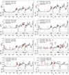 |
Fig. A.1. Best fits to the sample stars of Table 4 using the AGB models computed in this work (Table 2). The upper panels compare the [X/Fe] ratios as a function of the charge number Z, while the lower panels gives the deviations between the model and observation. The three best models are shown in black (lowest |


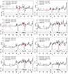 |
Fig. A.1. continued. |
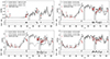 |
Fig. A.1. continued. |
All Tables
Overshoot coefficients used in the literature, at the bottom of the convective envelope (fenv) at the top of the convective pulse (ftop) and at the bottom of the convective pulse (fbot).
All Figures
|
Fig. 1. Kippenhahn diagrams showing the PIE in a 1 M⊙, [Fe/H] = −2.5 AGB model for three different values of the overshoot coefficient at the top of the convective pulse (ftop). Convective regions are shaded gray. The dotted green and blue lines trace the mass coordinate where the nuclear energy production by hydrogen and helium burning is maximum, respectively. The dashed green and blue lines delineate the hydrogen and helium-burning zones (where the nuclear energy production by H and He burning exceeds 10 erg g−1 s−1). The red areas show the extent of the overshoot zones. The black crosses indicates where and when the convective pulse splits. |
| In the text | |
|
Fig. 2. Evolution of maximal neutron density during a PIE. The different lines correspond to different values of the overshoot coefficient at the top of the convective pulse (ftop). The evolution is illustrated between the time t0 at which Nn, max rises above 1010 cm−3 and ends when the convective pulse splits. |
| In the text | |
|
Fig. 3. Neutron exposure at the bottom of the convective pulse (where the neutron density, Nn, is maximum) as a function of the ftop parameter. The color indicates the Zr (Z = 40) production factor, namely, its surface abundance normalized to its initial abundance. |
| In the text | |
|
Fig. 4. Impact of different overshoot parameters on the surface [X/Fe] ratios after a PIE in a 1 M⊙, [Fe/H] = −2.5 AGB model. Shown are the effect of including overshooting at the top of the convective pulse (panel a), at the bottom of the convective pulse (panel b), at the bottom of the convective envelope (panel c), when varying the parameters p (with ftop = 0.02 and ftop = 0.04, panel d), and Dmin with ftop = 0.02 (panel e), and ftop = 0.04 (panel f). The bottom subplots report the difference between a given model and the first model in the list. |
| In the text | |
|
Fig. 5. Final surface mass fractions (after decays) for the 1 M⊙ that experiences a PIE. The different colors correspond to the metallicities −0.5 (red), −1 (green), −1.5 (blue) and −2 (orange). Models were computed with ftop = 0.1. |
| In the text | |
|
Fig. 6. Final surface [X/Fe] ratios for the models that experience a PIE. The different panels correspond to different initial stellar masses. The various colors correspond to different metallicities [Fe/H] −0.5 (red), −1 (green), −1.2 (grey), −1.5 (blue), −2 (dark orange), and −2.5 (purple). All these models were computed with ftop = 0.1 A few models are not shown for clarity. |
| In the text | |
|
Fig. 7. Kippenhahn diagram showing the early AGB phase (first and second thermal pulses) of a 2 M⊙, [Fe/H] = −1.0 star (M2.0z1.0_f10 model). Convective regions are shaded gray. The dashed green and blue lines delineate the hydrogen and helium-burning zones, respectively (where the nuclear energy production by H and He burning exceeds 10 erg g−1 s−1). The red area shows the extent of overshooting. The magenta (cyan) line indicates the region zones where the i-process (s-process) nucleosynthesis occurs. The bottom panel shows the maximal neutron density as a function of the model number, or equivalently time as indicated in the upper x-axis. |
| In the text | |
|
Fig. 8. Abundance profiles of the M2.0z1.0_f10 model before the PIE (model 25344, panel a); right after the PIE (model 26044, panel b); just after the merging between the pulse and envelope (model 26544, panel c); at the end of the interpulse (model 42644, panel d); at the very start of the second thermal pulse (model 43586, panel e); and after the second weak PIE (model 44597, panel f). |
| In the text | |
|
Fig. 9. Elemental mass fractions at the surface of the M2.0z1.0_f10 model at three different times. The numbers in parenthesis correspond to the model number of Fig. 7. |
| In the text | |
|
Fig. 10. Surface [X/Fe] ratios in the M2.0z1.5_f10 model at four different times. Abundances are shown after the dredge up following the indicated pulse number (except for the black pattern that corresponds to the start of the AGB phase). |
| In the text | |
|
Fig. 11. Final elemental [X/Fe] ratios at the surface of the M3.0z2.5_f04 and M3.0z2.5_f10 models. |
| In the text | |
|
Fig. 12. Mass-metallicity diagram showing the occurrence of PIEs during the early AGB phase. The corresponding [Fe/H] ratios are indicated on the right axis assuming solar-scaled mixtures. Red filled circles show AGB models experiencing a PIE when ftop = 0. Empty black circles are for models that do not experience a PIE when ftop = 0. Thick black circles denotes models computed in this work and in Paper III. The small red circles and red dots highlight our models that experience a PIE when ftop = 0.04 and 0.10, respectively. The other models are from Iwamoto et al. (2004), Campbell & Lattanzio (2008), Cristallo et al. (2009a, 2016), Lau et al. (2009), Suda & Fujimoto (2010). The four colored zones show the approximate PIE zone when ftop = 0, 0.02, 0.04 and 0.10. |
| In the text | |
|
Fig. 13. Residual of the best fits for the 16 i-process stars candidates of Table 4. Black points correspond to MS and RG stars, while red points are for post-AGB stars. The crosses represent the average values of the residuals. The individual fits are shown in Figs. 14 and A.1. |
| In the text | |
|
Fig. 14. Best description of the RG star HE 2144−1832 (top panel) and post-AGB star J004441 (bottom panel) using the AGB models computed in this work (Table 2). The three best models are shown in black (lowest |
| In the text | |
|
Fig. 15. [La/Y] and [Ba/La] abundance ratios as a function of [La/Eu]. Circles correspond to MS and RG stars while squares are for post-AGB stars. Lines represent the dilution curves of the AGB material, which ultimately produce a material of solar composition (i.e., ratios equal to zero). Lines and symbols are color-coded according to the metallicity [Fe/H]. The small squares on the lines indicates where fdil = 0.9. The thick black line (bottom panel) shows a 2 M⊙, [Fe/H] = −2 model computed with a different set of neutron capture rates (see text for more details) and the red arrow shows the resulting abundance displacement. |
| In the text | |
|
Fig. A.1. Best fits to the sample stars of Table 4 using the AGB models computed in this work (Table 2). The upper panels compare the [X/Fe] ratios as a function of the charge number Z, while the lower panels gives the deviations between the model and observation. The three best models are shown in black (lowest |
| In the text | |
|
Fig. A.1. continued. |
| In the text | |
|
Fig. A.1. continued. |
| In the text | |
Current usage metrics show cumulative count of Article Views (full-text article views including HTML views, PDF and ePub downloads, according to the available data) and Abstracts Views on Vision4Press platform.
Data correspond to usage on the plateform after 2015. The current usage metrics is available 48-96 hours after online publication and is updated daily on week days.
Initial download of the metrics may take a while.