| Issue |
A&A
Volume 687, July 2024
|
|
|---|---|---|
| Article Number | A260 | |
| Number of page(s) | 17 | |
| Section | Stellar structure and evolution | |
| DOI | https://doi.org/10.1051/0004-6361/202449821 | |
| Published online | 18 July 2024 | |
The impact of overshoot on the i-process in AGB stars
1
Max-Planck Institut für Astrophysik, Karl-Schwarzschild-Str. 1, 85741 Garching, Germany
e-mail: This email address is being protected from spambots. You need JavaScript enabled to view it.
2
Ludwig-Maximillians-Universität München, Geschwister-Scholl-Platz 1, 80539 Munich, Germany
3
Excellence Cluster ORIGINS, Boltzmannstrasse 2, 85748 Garching, Germany
Received:
29
February
2024
Accepted:
12
April
2024
Abstract
Context. The production of neutron-rich elements at neutron densities intermediate to those of the s- and r-processes, the so-called i-process, has been identified as possibly being responsible for the observed abundance pattern found in certain carbon-enhanced metal-poor (CEMP) stars. The production site may be low-metallicity stars on the asymptotic giant branch (AGB) where the physical processes during the thermal pulses are not well known.
Aims. We investigate the impact of overshoot from various convective boundaries during the AGB phase on proton ingestion events (PIEs) and the neutron densities as a necessary precondition for the i-process as well as on the structure and continued evolution of the models.
Methods. We therefore analyzed models of a 1.2 M⊙, Z = 5 × 10⁻⁵ star. A fiducial model without overshoot on the AGB (overshoot was applied during the pre-AGB evolution) serves as a reference. The same model was then run with various overshoot values and the resulting models were compared to one another. Light element nucleosynthesis is also discussed. Additionally, we introduce a new timescale argument to predict PIE occurrence to discriminate between a physical and a numerical reason for a nonoccurrence. A comparison to observations as well as previous studies was conducted before finally presenting the most promising choice of overshoot parameters for the occurrence of the i-process in low-mass, low-metallicity models.
Results. The fiducial model reveals high neutron densities and a persistent split of the pulse-driven convection zone (PDCZ). Overshoot from the PDCZ results in either temporary or permanent remerging of the split PDCZ, influencing the star’s structure and evolution. While both overshoot and non-overshoot models exhibit PIEs generating neutron densities suitable for the i-process, they lead to varied C/O and N/O ratios and notable Li enhancements. Comparison with previous studies and observations of CEMP-r/s stars suggests that while surface enhancements in our models may be exaggerated, abundance ratios align well. Though, for high values of overshoot from the PDCZ the agreement becomes worse.
Key words: nuclear reactions / nucleosynthesis / abundances / stars: abundances / stars: AGB and post-AGB
© The Authors 2024
 Open Access article, published by EDP Sciences, under the terms of the Creative Commons Attribution License (https://creativecommons.org/licenses/by/4.0), which permits unrestricted use, distribution, and reproduction in any medium, provided the original work is properly cited.
This article is published in open access under the Subscribe to Open model.
Open access funding provided by Max Planck Society.
1. Introduction
The abundance of the elements in the Universe is the result of a rich number of nuclear processes occurring in a wide array of astrophysical sites. The elements heavier than iron are mainly produced by neutron captures. Two processes in particular are known to create roughly half of the trans-iron elements: the slow neutron-capture process (s-process) and the rapid neutron-capture process (r-process).
The r-process is characterized by a high neutron density, Nn > 1020 cm−1, occurring over a timescale of just seconds. The astrophysical site of the r-process is as of yet uncertain (Thielemann et al. 2011). In contrast, the s-process is identified with much lower neutron densities (Nn ≈ 106 − 1010 cm−3) and longer timescales. The s-process occurs in two different astrophysical sites. The so-called weak component of the s-process occurs in the core of massive stars during central helium burning as well as the carbon-burning shell in later nuclear burning phases. This component mainly produces elements with an atomic number A ≲ 90 and is powered by the 22Ne(α, n)25Mg neutron-source reaction (Karakas & Lattanzio 2014). The main component of the s-process, responsible for the creation of elements with an atomic number A ≳ 90, occurs in low- and intermediate-mass asymptotic giant branch (AGB) stars driven by the 13C(α, n)16O neutron-source reaction (Straniero et al. 1995; Gallino et al. 1998; Lugaro et al. 2003). In higher mass AGB stars it is possible that the 22Ne(α, n)25Mg reaction is activated as well (Iben 1975, 1982).
In addition to these two processes, Cowan & Rose (1977) proposed the idea of an intermediate neutron capture process, or i-process, which they claimed could occur in AGB stars during the thermal pulse. The i-process, as the name suggests, is defined by having neutron exposures intermediate to those of the s-process and r-process, Nn ≈ 1012 − 1016 cm−3. This idea has gained traction in the last two decades as observations have shown that there are many more extremely metal-poor (EMP) stars with strong carbon enhancement than predicted (Tomkin et al. 1989; Rossi et al. 1999; Aoki et al. 2007; Suda et al. 2011). These so-called carbon-enhanced metal-poor (CEMP) stars are further sub-categorized based on whether the surface abundances show no signs of enhanced neutron-capture-element abundances (CEMP-no), signs of s-process enhancement (CEMP-s), signs of r-process enhancement (CEMP-r), or signs of both r- and s-process enhancement (CEMP-r/s; Beers & Christlieb 2005). The i-process has been invoked to explain the abundance signatures of the CEMP-r/s stars as multiple studies have determined that these star’s abundances cannot be explained by a combination of r- and s-process yields (Jonsell et al. 2006; Lugaro et al. 2012; Dardelet et al. 2014; Hampel et al. 2016). Specifically, the Ba and Eu abundances of CEMP-r/s are difficult to explain using any combination of r- and/or s-process. The anomalous Ba enrichment in some open clusters has also been considered observational evidence of the i-process (Mishenina et al. 2015). In all cases the abundance of neutron-capture elements is assumed to be inherited from a previous generation of stars or a companion star. In the case of CEMP stars these elements would have come from a companion star that is now a white dwarf.
Though the astrophysical site at which the i-process occurs remains uncertain, the common thread among all of the hypotheses is the need for protons to be mixed to regions with He-burning temperatures and a sufficient abundance of 12C. This is in contrast to the s-process where protons need only be mixed into otherwise H-poor regions that have previously experienced He burning. The mixing of protons into a He-burning zone is generally referred to as a proton-ingestion event (PIE), but other names such as a H-ingestion event (HIE), He-flash driven deep mixing (He-FDDM), and dual flashes among others can be found in the literature1. The protons, having been mixed into a He-burning region, are captured by the abundant 12C to form 13C. The neutrons for the i-process are then released via the 13C neutron-source reaction which is very active at typical He-burning temperatures of 200 − 300 MK (Ciani et al. 2021). This results in neutron densities much higher than those of the s-process where the same reaction is occurring but at typical temperatures around 90 MK. A number of candidate astrophysical sites for the i-process have been put forth by various authors. The idea proposed in Denissenkov et al. (2017, 2019) is that the i-process occurs in rapidly accreting white dwarf stars. In this scenario the white dwarf is accreting proton-rich material from its binary companion. This proton-rich material is burned and forms He. Once enough He is formed, an unstable He-burning shell is created driving a convective zone that results in protons being mixed into the He-burning regions leading to i-process levels of neutron densities. Another possible site is the core helium flash of low-mass EMP stars when the flash-driven convection zone penetrates the H-rich region of the star (Fujimoto et al. 2000; Campbell et al. 2010; Cruz et al. 2013). Very late thermal pulses in AGB stars have been proposed, in particular in connection to Sakurai’s object (V4334 Sgr; Herwig et al. 2011). Super-AGB stars (AGB stars with initial masses between 7 M⊙ and 10 M⊙) have also been suggested (Jones et al. 2016).
In this work we focus on the final potential site, the thermally pulsing AGB (TP-AGB) phase of low-mass, metal-poor stars (Fujimoto et al. 2000; Iwamoto 2009; Cristallo et al. 2009; Suda & Fujimoto 2010; Choplin et al. 2021, 2022; Goriely et al. 2021). These stars are characterized by recurrent thermal pulses due to the thermonuclear runaway caused by the thin, unstable He shell. These periods of intense nuclear burning drive a convective zone between the He and H shells. At low metallicity this pulse-driven convection zone (PDCZ) can overcome the relatively small entropy barrier of the H shell and thereby mix protons to the base of the PDCZ to be burned. The penetration of the PDCZ into the H shell is possible at low metallicity as the dearth of metals, especially C, N, and O, leads to a reduced H-burning rate and thus reduces the entropy of the shell (Fujimoto et al. 1990). After the pulse has died down, the H shell, which acts as a barrier for the convective envelope (CE) just as it does for the PDCZ, is extinguished and the CE can then penetrate further into the star. In doing so the products of the nuclear burning, both standard He burning as well as neutron captures, if any, can be brought to the surface. This is known as the third dredge up (TDU) which is a common phenomena in many, if not all, TP-AGB stars.
There have been a number of studies of this i-process scenario. In Fujimoto et al. (2000) evolutionary models spanning a mass range of 0.8 − 5.0 M⊙ and a metallicity of [Fe/H] = −2 to 0 are computed. The models are split into 5 classes based on their behavior. In Case II′ which corresponds to [Fe/H] ≲ −2.0 and 1 M⊙ ≲ M ≲ 3 M⊙ their models exhibit a PIE. These stars are seen to evolve into more N-rich carbon stars with the additional enhancement of s-process elements. This work was later improved and extended in Suda & Fujimoto (2010) with a grid of models spanning masses of 0.9 − 9 M⊙ and [Fe/H] of −5 to −2 as well as 0. The region of the parameter space for case II′ is updated to be bounded by [Fe/H] ≲ −3 and 1.2 M⊙ ≲ M ≲ 3, M⊙. Detailed nucleosynthesis of the heavy elements is again not conducted, but they do state that the case II′ stars will again be N-rich carbon stars with s-process enhancement. A similar study was conducted by Lau et al. (2009) with qualitatively similar results. This is also the first study that attempts to include convective overshoot into the calculations. Unfortunately, numerical difficulties prevent them from drawing any firm conclusions but they claim that the subsequent evolution of the star will not be greatly affected by the use of overshoot and that it only shifts the range in parameter space where one would expect certain phenomena to occur. The AGB-scenario was also studied by Iwamoto (2009) but with a specific focus on Li and whether or not the Cameron–Fowler mechanism (Cameron 1955; Cameron & Fowler 1971) could operate during a PIE. At [Fe/H] ≈ −3 the models with M < 3 M⊙ undergo a PIE and produce large amounts of 7Li and 14N.
Detailed nucleosynthesis of PIEs in AGB stars have been calculated by a few authors including Cristallo et al. (2009) who investigate the i-process during a PIE in a M = 1.5 M⊙, Z = 5 × 10⁻⁵ ([Fe/H] = −2.44) model with a network of 700 isotopes and more than 1200 reactions. They find that the ingestion of H into the He shell causes a huge burst of energy from CNO-cycle burning. This energy eventually exceeds that of the triple-α reaction and creates a temperature inversion splitting the PDCZ into two separate convective zones that do not remerge. After the PIE, the star continues a regular AGB evolution experiencing further TPs and TDUs that dredge up material from the lower part of the split PDCZ.
Most recently, in a series of papers (Choplin et al. 2021, 2022; Goriely et al. 2021) the Brussels group investigate the i-process using a stellar evolution code with a fully coupled network of 1160 isotopes. The first paper provides an in depth analysis of a single evolutionary track for a 1 M⊙, [Fe/H] = −2.5 star. The authors find that a PIE occurs early in the AGB phase, in this case during the third pulse. The splitting of the convective zone is also seen in these models. This split occurs near but after the peak in the neutron density which reaches Nn = 4.3 × 1014 cm−3. After the PIE, the upper part of the split PDCZ merges with the CE and brings the i-process enriched material to the surface. Along with it comes a vast amount of carbon raising the surface 12C abundance by over 3 dex. Thus, the star becomes a carbon star triggering rapid mass loss that ends the AGB before any further pulses can occur. Another key aspect of this first paper is a test of the dependency of the PIE on the spatial and temporal resolution of the simulation. The tests show that if the spatial or temporal resolution is too coarse it is possible to miss the PIE entirely and have the star evolve along a typical AGB evolution path.
The second paper of the series concentrates on the nuclear uncertainties and their effect on the i-process and PIEs. They conclude that in general the final elemental surface abundances are uncertain within ±0.4 dex due to the nuclear uncertainties. Interestingly, the uncertainty related to the 13C neutron source reaction rate and the β-decay rates have only a minor impact on the final surface abundances. Of course this may be different if one were able to compare to isotopic rather than elemental abundances.
The third paper presents a grid of models with initial masses of 1, 2, and 3 M⊙ and metallicities of [Fe/H] = −3.0, −2.5, −2.3, and −2.0. PIEs occur in their models with masses of 1 M⊙ and 2 M⊙ and with metallicities of [Fe/H] = −3, −2.5, and −2.3 during the first or second thermal pulse. The peak neutron density remains relatively unchanged over this parameter range with Nn = 1014 − 1015 cm−3. They find that the PIE effectively terminates the AGB phase for their 1 M⊙ models, but the 2 M⊙ models continue along the AGB after the PIE. The authors expect that this is due to the larger envelopes (in mass) of the 2 M⊙ stars which dilutes the carbon enrichment and thus avoids triggering the rapid mass loss that goes along with a high C/O abundance. None of their models with a mass of 3 M⊙ or a metallicity of [Fe/H] = −2.0 experience a PIE as the entropy barrier of the H shell is too large in these stars.
Recently, the pre-print of another paper from this group on the impact of overshoot on the i-process in AGB stars was released with a particular emphasis on the heavy element abundances (Choplin et al. 2024). Various overshoot values for the top and bottom of the PDCZ as well as the convective envelope are tested on their standard 1 M⊙, [Fe/H] = −2.5 model. Because of long computation times the calculations of these models are not actually completed, though. They only carry out the calculations until the PDCZ splits at which point they apply a procedure to approximate the final surface abundances without having to carry through with the modeling. They find that overshoot at the top of the PDCZ, for which they vary the extent from 0.0 to 0.2 scale heights, plays the most important role in whether the PIE occurs and in the final surface abundances. Overshoot at the bottom of the PDCZ and the convective envelope are considered far less important.
A common aspect of all but one of these studies was the strict application of the Schwarzschild criterion in determining the extent of the convective zones. However, it is well understood that extra-mixing processes play a crucial rule in the modeling of AGB stars (Herwig 2005; Wagstaff et al. 2020). In this work we aim to investigate the impact of applying overshoot at various convective boundaries. We focus on the structural and evolutionary aspects, deferring the nuclear synthesis to a future paper. In particular we investigate the splitting of the PDCZ, the final surface abundances of light elements, and provide estimates of the neutron densities as a first indication of the nuclear synthesis. All the evolutionary tracks run in this work are for a Minitial = 1.2 M⊙ star with Z = 5 × 10⁻⁵ ([Fe/H] = −2.56) unless otherwise specified. Furthermore, all models were run until the envelope was almost entirely lost due to winds at which point convergence issues prohibited any further calculations. This is a known issue in modeling AGB stars (see Wood & Faulkner 1986; Lau et al. 2012)
2. The stellar models
For the purposes of generating the stellar evolution models for this work the GARching STellar Evolution Code or |GARSTEC| (Weiss & Schlattl 2008) was used. |GARSTEC| is a general purpose stellar evolution code capable of calculating stellar models from the pre-main sequence to the early white-dwarf stage for low-mass stars, or carbon burning for higher mass stars. More information on the specific workings of the code can be found in Weiss & Schlattl (2008)2. All models were run with a solar calibrated mixing length of α = 1.68 and using the OPAL-EoS equation of state (Rogers & Nayfonov 2002). The solar abundance was assumed to be that of Grevesse & Sauval (1998). Because tests by Choplin et al. (2021) found very little impact on the PIE when using alpha-enhanced mixtures, we ignored deviations from the solar metal ratios. What follows is a brief discussion of the most relevant input physics which is varied in this study.
2.1. Convective overshooting
Convective overshooting, whether in the form of material overshooting the boundary or other proposed extra mixing mechanisms, is a physical process that certainly takes place at all convective boundaries. In |GARSTEC|, convection is handled by the standard mixing-length formulation of Kippenhahn et al. (2013). Convective overshooting is implemented with the description by Freytag et al. (1996). Their description of overshoot is based on a diffusive mixing model which is incorporated into |GARSTEC| with a diffusion coefficient,
 (1)
(1)
where fov is the free parameter, z is the radial distance from the Schwarzschild boundary (Schwarzschild 1906), Hp is the pressure scale height at the Schwarzschild boundary, and D0 is the value of the diffusion constant close to the Schwarzschild boundary. Since in mixing-length theory D0 is formally zero at the Schwarzschild boundary different codes define it in different ways. In |GARSTEC| D0 is defined as the diffusion constant, as calculated in mixing-length theory, at 0.5Hp inside the edge of the convective zone.
Using this overshoot description, problems may occur when running models for stars with very small convective cores. As Hp grows ever larger toward the center of the star, the overshooting region would become unrealistically large. This is handled in |GARSTEC| by applying a geometrical cut-off. In Eq. (1), Hp is replaced by
![Mathematical equation: $$ \begin{aligned} H_p^* = H_p \min \left[1,\frac{\tanh \left(5\left(\frac{\Delta R_{\mathrm{CZ}}}{H_p}-1\right)\right)}{2} + 0.5\right], \end{aligned} $$](/articles/aa/full_html/2024/07/aa49821-24/aa49821-24-eq2.gif) (2)
(2)
which ensures that the overshooting region is restricted to a fraction of the radial extent of the convective zone, ΔRCZ. This specific analytical form for the cut-off provides consistency between core sizes in |GARSTEC| models and observations from open clusters and detached eclipsing binaries independent of main-sequence mass.
As an additional extension to the AGB branch of the code the option for setting different overshoot parameters for different convective boundaries was implemented (Wagstaff 2018; Wagstaff et al. 2020). During the course of the life of a star many different convective zones will come and go. Normally, the same overshoot value is used for all convective zones and applies to both over and undershooting – overshooting from the upper and lower convective boundaries, respectively. There is, however, no reason to think that this overshoot parameter would be the same for qualitatively different convective zones or even for the over and undershooting of the same convective zone due to the different thermal and structural conditions (see, e.g., the discussions in Miller Bertolami 2016 and Wagstaff et al. 2020). Separate overshoot parameters can be set for the core convective zone during H burning (|fCHB|), the core convective zone during He burning (|fCHeB|), the bottom of the convective envelope (|fCE|), the bottom of the PDCZ (|fPDCZb|), and the top of the PDCZ (|fPDCZt|). For the current study the values of |fPDCZt| and |fPDCZb| are always equal and thus will be referred to jointly as |fPDCZ|. The values used for the various overshoot values in this study will be given in Sect. 3.
2.2. Nuclear network
In the AGB branch of |GARSTEC| the nuclear network has been expanded. This was originally started as part of the work in Cruz et al. (2013) and was further improved for this work. This was necessary in order to account for the neutron sources and neutron poisons important for the i-process. Additionally, more isotopes were needed to follow the energetics of nuclear burning processes during the PIEs.
The new network includes 19 more isotopes than the old one for a total of 30 isotopes with 119 reactions. See Fig. 1 for an overview of the two networks. It is clear that this network is insufficient to follow the neutron capture reactions, but its accuracy for the isotopes it includes has been confirmed by testing it against the full nuclear network in ANT (Battich et al. 2023). Not pictured in the diagram is the neutron sink which is used to mimic the neutron capture cross section of all elements not included in the network and is implemented in the way described in Cruz et al. (2013). Briefly, the number abundance and neutron-capture cross-section of the neutron sink, denoted as 30AA, are given as
 (3)
(3)
 (4)
(4)
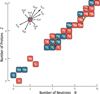 |
Fig. 1. Depiction of the nuclear network of |GARSTEC| in this work. The blue squares represent those isotopes that are in the nuclear network in the main branch of |GARSTEC|. Red isotopes are ones that have been added to the network in the AGB branch. As is standard practice we have included both the ground state and the isomeric state of 26Al. The main neutron source reactions and the primary neutron poison reaction are marked with arrows. |
respectively, where Ni are the number abundances of isotope i, Yi are the mole fractions of isotope i, and the summation extends over all isotopes not included in the network in the stellar evolution code. The difficulty in this approach is that the neutron sink cross-section,  , must be known ahead of time. This is done by running detailed calculations with a full nuclear network to provide estimates for its value at different neutron exposures (Cruz et al. 2013). The neutron exposure, τ, can be calculated as
  where Nn is the neutron density and vT is the thermal velocity of neutrons at temperature T. A detailed study of the nucleosynthesis using a post-processing nuclear network will be done in a future study. As such all values for the neutron densities and neutron exposures are estimates based on our neutron sink approach.
The reaction rates used by |GARSTEC| in this work come from different sources. With a few exceptions the rates come from either the NACRE collaboration (Angulo et al. 1999; Xu et al. 2013) or the recommended JINA Reaclib database rates (Cyburt et al. 2010). The important exceptions are listed below:
-
13C(α, n)16O (Ciani et al. 2021)
-
22Ne(α, n)25Mg (Jaeger et al. 2001)
-
12C(α, γ)16O (Kunz et al. 2002).
2.3. Opacities
During the TP-AGB phase, the star may undergo a number of TDU events. These events will dredge-up the products of various nuclear burning processes including the i-process. In particular, large amounts of C will be brought to the surface. Over the course of the AGB phase the C in the outer layer will build up until the C/O ratio exceeds unity; the star is now what is called a carbon star. In order to better model the outer layers in this phase one needs opacity tables for which C/O takes different values. Without doing so you will underestimate the opacity (Marigo 2002). This in turn leads to an overestimation of the effective temperature and an underestimation of the mass loss rate.
Kitsikis & Weiss (2007), Kitsikis (2008) and Weiss & Ferguson 2009 discuss the addition of C/O variable opacity tables to |GARSTEC| and their effect. These low-T opacities were provided by J. Ferguson from Wichita State University (WSU; Ferguson 2006, priv. comm.) and combined with high-T opacity tables for identical mixtures from Iglesias & Rogers (1996). The C/O values for the tables are 0.17, 0.48, 0.9, 1.0, 1.1, 3.0, and 20.0, with |GARSTEC| being able to choose the appropriate one based on the current abundances at every time step.
2.4. Mass loss
Mass loss can not be ignored when modeling these stars. The mass loss rates can reach extreme values of up to 10−4 M⊙ yr−1 and is critical in determining the lifetime of the AGB phase. We take the same approach for mass loss as in Kitsikis & Weiss (2008) and Wagstaff (2018). In short, Reimers’ wind (Reimers 1975) was used on the red giant branch (RGB) with ηR = 0.4. Once on the AGB, one of three formulas was used. If the period, estimated by
 (5)
(5)
as determined by Ostlie & Cox (1986) on the basis of linear pulsation, is less than 400 days then Reimers’ wind is used. If the period exceeds this value, the prescription of van Loon et al. (2005) was used for O-rich stars and the prescription of Wachter et al. (2002) was used for C-rich stars.
3. Results
3.1. Fiducial model: M = 1.2 M⊙, Z = 5 × 10⁻⁵
We begin by discussing in detail the evolution of a Minitial = 1.2 M⊙, Z = 5 × 10⁻⁵ ([Fe/H] = −2.56) evolutionary model. These values were chosen to allow for a comparison to Cristallo et al. (2009) and Choplin et al. (2021) (see Sect. 4.2). For this model overshoot was only applied to the convective core with overshoot parameters of |fCHB| = |fCHeB| = 0.016. This value is calibrated to match observations of main-sequence stars in clusters (Maeder & Meynet 1991; Stothers & Chin 1992; Weiss & Schlattl 2008; Magic et al. 2010). There is no clear way of calibrating the core overshoot for the horizontal branch so the typical practice is to use the same value as for the main sequence (Wagstaff et al. 2020). It should be mentioned that there are studies which would suggest, based on model matching to asteroseismology observations, that higher or lower values of fov are needed during the central He burning (Bossini et al. 2017; Brogaard et al. 2023). This model will act as a fiducial model for comparing what happens when we add or change the physics in other models.
3.1.1. pre-AGB
The evolution up to the AGB phase proceeds in the expected manner. On the main sequence the hydrogen burns radiatively in the core until the fuel runs out at the age of 2.5 Gyr. The star then ascends the red giant branch and experiences the He flash before settling on the horizontal branch burning He in its core for another 100 Myr.
3.1.2. The AGB
The TP-AGB phase for this star begins as any other with a typical cycle of H-shell burning, He flash, PDCZ, and interpulse phase. The H-free core mass of this model just before the first instability is 0.53 M⊙. The first instability is rather weak with He luminosities only reaching log LHe/L⊙ = 5.6. The relatively weak flash is nevertheless strong enough to drive a PDCZ. The convective envelope does intrude into the star post-PDCZ but not enough to cause a TDU event. After this flash there is a subflash with an even lower luminosities and smaller PDCZ. This is something we see in all of our models for the first few instabilities, after which the subflashes disappear. This is a known phenomenon (see, for example, Sackmann 1977).
The second instability is more standard. The He luminosity exceeds log LHe/L⊙ = 6.5 and drives a PDCZ spanning over 3.0 × 10⁻² in mass after which the envelope again extends deeper into the star, though still insufficiently far for TDU. A short while later there is a weaker subflash again producing a small PDCZ.
The third instability is where the PIE occurs. This flash is again stronger than the previous ones with He luminosities over log LHe/L⊙ = 7.2 even before the PIE. As the PDCZ expands in response to the energy release at its base, its outer border begins to eat into the H-rich region bringing protons to the base of the PDCZ. Here temperatures are in excess of 200 MK and the protons can very quickly be captured by 12C to create 13C. 311 yr after the pulse began the neutron density exceeds 1011 cm−3 marking the beginning of the i-process conditions. The neutron densities steadily increase for the next 150.56 days before reaching its maximum of 9.15 × 1014 cm−3. Shortly after, the H luminosity reaches its maximum, approaching log LH/L⊙ = 10.42, and the He luminosity exceeds log LHe/L⊙ = 8.18. However, the luminosity maxima do not occur at the same time; the He luminosity reaches its maximum slightly before the H luminosity. The run of the luminosity during the PIE can be seen in Fig. 2.
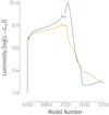 |
Fig. 2. Time evolution of the H luminosity (in blue) and the He luminosity (in orange) of the fiducial model during the PIE. |
1.14 hr before the neutron densities reach their maximum the PDCZ splits in two. The lower convective zone is the site of the maximum neutron density and therefore a large part of the nucleosynthesis occurs here after the split. Furthermore, the upper and lower convective zones never remerge throughout the evolution meaning that any nucleosynthetic products that are made in the lower convective zone remain trapped there for now. The upper convective zone, which contains some of the products of the nucleosynthesis prior to the split, merges with the CE a few years after the split and leads to clear surface enhancements. Because of the split, the effective time over which the i-process can occur is reduced to 150.59 days. The split occurs when the rate of the 12C(p, γ)13N reaction is approximately equal to the local convective turnover timescale (Cristallo et al. 2009; Choplin et al. 2021). The same pulse was calculated multiple times with varying temporal and spatial resolution settings and it was found that regardless of the settings the split happens before the maximum neutron density for this star, though the details of the PIE, such as neutron exposure, do change with changing resolution.
As already stated, a few years after the convective zone splits the nucleosynthetic products are dredged up to the surface of the star when the upper convective zone merges with the convective envelope. This drastically changes the surface abundances of the model. The C/O ratio reaches a value of 19.26 making it a very carbon-rich star. The large C/O ratio heralds the beginning of the end for the AGB phase for the star as it triggers intense mass loss from the envelope of the star (Ṁ ≲ 1 × 10⁻⁵ Ṁ−5 yr−1). The erosion of the envelope happens quickly, but not so quickly as to impede further thermal pulses. The star goes on to have three additional pulses before the envelope is completely stripped. A rather deep TDU is experienced in the pulse immediately after the PIE but not in the further two TPs. The TDU will have an important consequence for the final surface abundances of the neutron-capture elements as it will be able to dredge to the surface some of the nucleosynthetic products from the lower part of the split PDCZ that would have otherwise remained trapped deep inside the star. This is a two-part process. First, the nuclear burning products produced in the lower part of the PDCZ of the previous pulse will be mixed throughout the intershell by the post-PIE PDCZ. Next, the deep TDU will carry some of the intershell material to the surface. The TDU does not actually reach the mass coordinate where the lower part of the PDCZ was during the PIE.
One thing that is clear from the evolution of this star is the rapidity with which the PIE and subsequent nucleosynthesis occurs. From Fig. 3 one can see that the time between the PDCZ approaching the base of the H shell and the maximum in the neutron density is on the order of a year which is in agreement with Choplin et al. (2021). Because of this, the time-stepping as well as the spatial resolution of the stellar evolution code has grave consequences. During the PIE the time step taken by |GARSTEC| can reach the level of hours and does not exceed 10−4 yr at any point during the PIE. In our tests for this particular model we find that the occurrence of the PIE is not particularly sensitive to the spatial resolution of our models (though, quantitatively the characteristics of the PIE are different with lower resolution). It is however sensitive to the temporal resolution. There are many ways to control the time stepping in |GARSTEC|. After setting the minimum and maximum allowed time step one can also restrict the amount by which various quantities, for example luminosity, effective temperature, pressure, etc., change between two models. In the end it was found that specifically the size of the allowed changes of the H and He luminosity were key. If larger jumps in the H and He luminosity are allowed between models the PIE will be missed entirely and the star will evolve as a normal AGB star as was also see in Choplin et al. (2021).
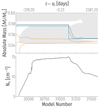 |
Fig. 3. Kippenhahn diagrams showing the structure of the fiducial model (top) and the maximum neutron density (bottom). Time is shown as model number on the lower x-axis and as time in days relative to the maximum neutron density in the upper x-axis. In the Kippenhahn diagram the top and bottom of the H shell is denoted by the solid blue lines with the dotted blue line following the point of maximum H burning in the shell. The top and the bottom of the He shell is denoted by the solid orange lines with the orange dashed line following the point of maximum He burning in the shell. Formally Convective regions are shown in gray. |
3.2. Including overshoot on the AGB
With the fiducial model described in detail we can use it as a point of comparison for the models that include overshoot on the AGB. Recall that we only vary overshoot parameters on the AGB; all models had overshoot included for core convective zones in earlier phases of the evolution. The key results for all models discussed in this section can be found in Table 1.
Selected key results of the stellar evolution models for all the tracks discussed in this section.
3.2.1. Overshoot from the CE only
We begin our discussion of this section by looking at those tracks where overshoot was only applied at one boundary. In doing so we can hope to isolate the effect of overshooting at each boundary on the variables of interest. Starting with overshoot from the CE, one can see in Table 1 that there appears to be an anti-correlation between |fCE| and the maximum neutron density, though the effect is minimal. Additionally, the neutron exposure, τ, defined here as the neutron flux integrated over the time between the beginning of the pulse and the split of the PDCZ, also exhibits an anti-correlation with |fCE|. As one would expect, with increasing |fCE| the final surface C/O ratio increases, though not monotonically. Interestingly, this increase in the surface C/O is not sufficient to suppress the post-PIE TPs seen in the fiducial model because the increase in C/O is fairly small. Furthermore, all of these tracks experience a rather deep TDU in the TP immediately following the PIE, but not in any of the later TPs. Finally, as with the fiducial model, the PDCZ split always occurs before the maximum neutron density is reached.
3.2.2. Overshoot from PDCZ only
This situation changes for those tracks with only PDCZ overshoot. While the PDCZ does indeed split before the maximum Nn for all but one track, the upper and lower convective zones do remerge either temporarily or permanently before the upper convective zone merges with the CE. It should be noted here that, although we refer to this as a remerging, in some cases the formal convective zones, as defined by the Schwarzschild criterion, remain separate and it is only the overshoot region which bridges the gap between the two convective zones. The remerging of the convective zones occurs as the H luminosity is decreasing after its peak. This means that the nucleosynthetic products that were formed in the lower part of the split PDCZ are not trapped there in these models and that some of the products can make their way to the surface. In this case the neutron exposures reported for these tracks are calculated from the beginning of the pulse to the time when the PDCZ splits for the final time or when the neutron densities fall below 1011 cm−3, whichever happens first. The efficiency of the mixing between the convective zones is not considered when classifying whether the zones have remerged or not. An example of a partial remerging can be seen in Fig. 4a around model 23 800. None of these models experience any post-PIE TPs. For these models there is again a negative monotonic relationship between the overshoot and the neutron exposure, with increasing |fPDCZ| the neutron exposure will decrease. Additionally, the final C/O value is much smaller in these tracks than in the previously discussed ones and decreases with increasing |fPDCZ|. This is not surprising as it is well known that overshoot at the base of the PDCZ alters the intershell composition. The larger the overshoot the more He is brought into the PDCZ from below. This leads to stronger flashes with higher temperatures which in turn increases the O/C ratio (Herwig 2000). This material is then dredged-up to the surface and results in a less carbon rich surface.
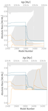 |
Fig. 4. Kippenhahn diagrams (see Fig. 3 for an explanation of the plot elements) of a PIE. Top panel: the |fPDCZ| = 0.016, |fCE| = 0.016 track experiences a partial remerging that occurs around model 23 800. Additionally, one can see the dredge-up-like event that happens when the upper part of the split PDCZ descends into the region below the split point. Bottom panel: the |fPDCZ| = 0.016, |fCE| = 0.016 track without the geometrical cut-off to the overshoot experiences a permanent remerging. |
3.2.3. Overshoot at all boundaries
The more internally consistent approach would be to apply overshoot at both the CE and the PDCZ which will be discussed now. These tracks follow the same trends as seen in the those tracks where overshoot is only applied to one boundary and their properties can largely be understood as a composite of those of the previous two sections. However, a few points bear mentioning. First, none of these tracks have any post-PIE TPs, consistent with the |fPDCZ|-only tracks. Second, for each of these tracks the PDCZ splits before the maximum Nn but later remerge temporarily or permanently. Third, the maximum neutron densities and the neutron exposures are all smaller for these tracks as compared to the fiducial model and the tracks with only overshoot at the CE. Finally, in addition to the remerging of the split PDCZ the tracks also experience a sort of dredge-up event. After the PIE and before the remerging, the upper part of the split PDCZ penetrates below the mass coordinate where the PDCZ split occurred and thus partially dredges-up the material from the lower CZ (see Fig. 4a). The greater |fPDCZ|, the deeper below the PDCZ split point the upper CZ can reach.
As a final point in this section there is the need to discuss a few numerical aspects of the overshooting implementation of |GARSTEC|. First, as mentioned in the beginning of this section, overshoot was applied to only the base of the CE and to the PDCZ. This strict application of overshoot has a drawback. When the PDCZ splits only one of the split zones will be identified as the PDCZ and have overshoot applied to its boundaries. The other split zone will have no overshoot. A second numerical aspect of overshooting in our code is the convective zone cutoff described in Sect. 2.1. As mentioned in that section, the geometrical cutoff is implemented to prevent small convective cores from growing unrealistically large. This is a common feature in stellar evolution codes, though the exact implementation differs (for a discussion see Sect. 2.7 of Anders & Pedersen 2023). However, during the simulations the overshoot regions of the two parts of the split PDCZ were at times also being cutoff due to this technique. It was prudent to see what would happen if either the geometrical cutoff was removed or if overshoot was applied to both parts of the split PDCZ for these tracks for the AGB phase. The effect of either of these changes is similar and so we focus on the case where the geometric cutoff is removed. In Table 1 one can see the results for these tracks, which have been marked with the † symbol. The most important characteristic of these tracks is that the PDCZ splits but does so after the maximum of the neutron density. Furthermore, the split PDCZ does remerge permanently and ultimately also remerges with the envelope such that one has a CZ that extends from the surface of the star to the base of the He shell. An example of such a track can be seen in Fig. 4b.
This seems to have a smaller than expected impact on the key features of the track. The maximum neutron density and neutron exposure do increase, but only by around ten percent. This is because the split of the PDCZ occurs very close to the maximum neutron density for the tracks with the geometric cutoff and thus the PDCZ material is subjected to the bulk of the neutron exposure regardless of whether the PDCZ remerges or not. Additionally, the final surface C/O is also slightly reduced.
3.3. The surface abundances
Table A.1 shows the final surface abundances of some key light elements for every track in this study in mass fraction and [X/H]3. As previously stated, the models were run until the envelope was almost entirely lost due to winds at which point the models fail to converge. C/O has already been discussed in the previous section and as such will not be addressed further here. It is only included in the table for completeness. Focusing first on the CNO elements one can see that only those tracks without any overshoot for the PDCZ have a N/O ratio greater than 1. The N/O ratio changes mostly due to the abundance of O. As has already been mentioned once before, the higher |fPDCZ| is, the higher the temperature of the He burning and the higher the O/C will be. Ultimately, this means that the surface of the star will have more O enhancement. This can easily be seen in the table as well.
7Li also has a very strong surface abundance enhancement. The network was not applied to grid points below a certain temperature and thus the 7Be(e−, ν)7Li reaction was not active in the envelope in the later stages of the AGB evolution after the PIE. For this reason in Fig. 5 we plot the sum of 7Li and 7Be as a proxy for 7Li as all the 7Be would be expected to become 7Li. Test calculations were conducted for one model with a lower temperature cutoff to ensure that this is indeed the case. In Table 2 and for the remainder of the paper it is understood that when we discuss the Li abundances we are in fact discussing this sum of Li and Be abundances. The high Li abundance indicates that the Cameron–Fowler mechanism (Cameron 1955; Cameron & Fowler 1971) is at work in these stars. At the point when the upper part of the split-PDCZ merges with the envelope, the H shell is still burning at the base of the now merged convective zones. Here the temperature is 50 MK just after merging and decreases over time. This means that there is a brief period of hot-bottom burning but also a brief window in which 7Be can be produced and convectively transported to the surface layers where it captures an electron to form 7Li. We do not see evidence that the Li is then later destroyed; The abundance at the surface remains constant and the Li is carried off in the winds.
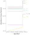 |
Fig. 5. Time evolution of the surface abundances (in mass fraction) of certain elements for the |fPDCZ| = 0.008, |fCE| = 0.000 track. |
Key characteristics of the observed CEMP-r/s stars used in this study.
The heavier elements are far less affected by the PIE. Sodium is enhanced in all tracks, with the |fPDCZ| = 0 tracks being the most enhanced. Magnesium and aluminum on the other hand show little to no deviation across the overshoot parameter space. However, as one can see in Fig. 5, the envelope does experience a rather large enrichment in the isotope 26Alg. This is a sign of H burning at temperatures above approximately 100 MK (Ventura et al. 2016). Indeed during the PIE the temperatures in the H burning shell exceed 150 MK allowing for the synthesis of 26Alg.
4. Discussion
4.1. To ingest or not to ingest
4.1.1. The entropy argument
One of the key concerns when running these low-mass, low-metallicity models is whether a PIE should occur or not. If a PIE does not occur during a particular TP in a model it is unclear if that is because of a lack of resolution or because it physically should not occur. There is currently no consensus in the literature on how to determine whether a PIE should happen for a particular TP. Most of the arguments are based on the idea of an entropy barrier (Fujimoto et al. 1990; Iwamoto et al. 2004; Choplin et al. 2022). Namely, that one can calculate the entropy barrier between the edge of the PDCZ and the base of the H-rich region and then compare this value across models and pulses to determine a critical entropy barrier value below which a PIE will occur; This is the approach taken in Choplin et al. (2022). While they do find a critical value below which PIEs occur, they advise caution for a number of reasons: it only gives a good hint as to whether a PIE should occur, the metallicity dependence is not straight forward, and there are different criteria one can use to estimate the value of the entropy barrier. Additionally, the exact value is likely to be code dependent and thus requires running a grid of models over a parameter space to determine the critical value.
4.1.2. The timescale argument
Our approach is to use timescale estimates to establish a criteria for whether a PIE occurs or not. This approach has been successfully used in the past to estimate the extent of the PDCZ (Despain & Scalo 1976; Fujimoto 1977).
In Despain & Scalo (1976) they argue that the quenching of the flash is due to a thermal adjustment and not a hydrostatic one as is the case with the core-He-flash convection zone. During a pulse, they argue, the intershell region does expand hydrostatically but this expansion has little impact on the layers above the H shell because they are hydrostatically decoupled from the intershell. This decoupling is due to the energy generation in the H shell that provides a strong restoring force against perturbations in radius (Stein 1966). However, the thermal perturbations of the He shell can be communicated to the outer layers by means of radiative diffusion.
They define a timescale for the growth of the perturbation, τHe, and a timescale for radiative diffusion from the He shell to the H shell, τdiff. As long as τHe < τdiff the PDCZ will grow because the instability is growing faster than the outer layers can receive the information, but when τHe ≈ τdiff the outer layers can respond to any changes from the He shell as quickly as they occur and the PDCZ will cease to grow. Their numerical simulations support this argument and they find that a sufficiently violent flash would cause the intershell convective zone to make contact with the H-rich layer. One year later Fujimoto (1977) carried out a similar analysis, though, the timescales were defined slightly differently. Regardless, their computations also support the argument of Despain & Scalo (1976).
4.1.3. An update to the timescale argument
In the present study the timescales are defined as
 (6)
(6)
 (7)
(7)
where the angled brackets denote an average over the PDCZ, Cp is the specific heat capacity, Mconv is the mass of the PDCZ, and srad is a quantity defined in Sugimoto (1970) as

and represents the non-dimensional entropy of radiation. τdiff is evaluated one grid point beyond the upper boundary of the PDCZ. These are almost identical to the definitions used in Fujimoto et al. (1990) with the only difference being the convective-zone averaging of the specific heat capacity.
To these timescale we also add a third, τH, that is defined exactly as in Eq. (7) but evaluated at the base of the H-rich region which we defined as the point below the H shell where the mass fraction of hydrogen drops below 0.15. The exact value of τH is only weakly sensitive to how one defines the base of the H-rich region. Changing the critical value of the hydrogen abundance to 0.1 or 0.2 only results in a change in τH of approximately two percent.
4.1.4. Model investigations of timescales
We first look at how these quantities vary for pulses where one would not expect a PIE. In Fig. 6 one can see the evolution of the timescales during the third thermal pulse for a 3 M⊙, solar metallicity star (Fig. 6a) and a 1.2 M⊙, Z = 5 × 10⁻⁴ model (Fig. 6b; metallicity being ten times higher than in the fiducial model).
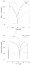 |
Fig. 6. Time evolution of the three timescales, τHe, τdiff, and τH, for the third thermal pulse in a 3 M⊙, solar metallicity model (top) and a 1.2 M⊙, Z = 5 × 10⁻⁴ model (bottom). No PIEs are expected for stars with these parameters. The zero point for time in the x-axis is the point when the PDCZ first appears for this pulse. |
In both cases one can see that τHe first decreases as the pulse strengthens due to the increase in the luminosity of the He shell. The peak He luminosity is achieved as τHe arrives at its nadir, at which point the He luminosity decreases and τHe in turn increases again. Shortly after this minimum, the criterion τHe ≈ τdiff is fulfilled and the PDCZ reaches its maximum extent. τdiff evolves in a similar fashion where at first it decreases due to the decrease in density and increase in temperature just beyond the edge of the PDCZ. After the PDCZ reaches it maximum extent the layers above the PDCZ cool again leading to the increase of τdiff. In contrast τH remains rather constant over the course of the pulse, only slightly increasing as the PDCZ reaches its maximum extent. No PIE is expected in either of these cases.
In Fig. 7 we see the same type of plot as in Fig. 6, this time both panels show the third TP of the same, more metal-poor star: a 1.2 M⊙, Z = 5 × 10⁻⁵ star. In the upper panel is the model for which the time resolution was insufficient to resolve the PIE and in the lower panel is the fiducial model where the PIE is resolved. Comparing these plots to those from Fig. 6 one can see that there is a condition that is satisfied here that is not satisfied in the previous models: τHe < τdiff ≲ τH. Even in the model for which the PIE is missed this condition is briefly fulfilled. In the model where the PIE does occur the PIE begins exactly when τHe < τdiff ≃ τH is true. Furthermore, for the low-resolution model where the PIE is missed, this condition is fulfilled for pulses three through six but not for any of the later pulses. This is in agreement with the expectation that PIEs are only possible in the first few thermal pulses (Choplin et al. 2022). It should also be noted that it was checked that even when τdiff = τH they are not being evaluated at the same grid point and so the equivalency is not trivial.
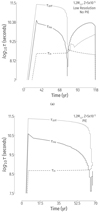 |
Fig. 7. Time evolution of the three timescales, τHe, τdiff, and τH, for the third thermal pulse of the 1.2 M⊙, Z = 5 × 10⁻⁵ model with poor temporal resolution (top) and the fiducial model (bottom). In the upper panel the code has missed the PIE due to poor time stepping while in the lower panel the PIE was resolved. The zero point for time in the x-axis is the point when the PDCZ first appears for this pulse. |
Comparing the timescales in Figs. 6 and 7 one can see that τH increases in relation to the other timescales as both the metallicity and mass decrease. The dependence of the timescales on mass and metallicity can be explained as follows. The argument hinges on the fact that burning shells provide strong restoring force to perturbations in radius, and mass shells without burning will simply expand or contract with the rest of the star (Stein 1966). This implies that the behavior of τdiff will not change much across metallicity and mass because the expansion of the intershell will proceed similarly in all cases. This can be seen by comparing Figs. 6 and 7. The behavior of τH will change though as the luminosity of the H shell (and thus the energy generation) is much lower during the flash at lower metallicity which, in turn, means it resists changes in radius less. This means the expansion of the H shell outward will begin earlier in the pulse. This pushes the base of the H-rich region further out as well as it will simply expand with the layers above and below it. Here the radius will be higher and T will be lower than it otherwise would be and hence τH will be higher. To check this the PIE pulse was run again but with the CNO burning rates increased by a factor of ten. This increases the luminosity of the shell and in turn increases the tendency of the shell to resist any change in radius. This keeps τH low enough that it never exceeds τdiff and the PIE never occurs. Of course increasing the CNO rates also impacts the temperature in the shell and it is difficult to disentangle these simultaneous effects to determine which one is truly responsible for the suppression of the PIE. That being said, the ten times increase in the CNO reaction rates leads to a near 100% increase in the H luminosity and only a 25% increase in the H shell temperature near the time when the PIE would occur. Finally, the behavior of τHe is the easiest to explain as it is primarily dependent on the He luminosity. Thus, its dependence on mass on metallicity exactly follows that of the He shell luminosity for AGB stars: τHe will decrease with increasing mass and decreasing metallicity.
All of this applies specifically to tracks without overshoot from the PDCZ. The criterion still works for those tracks with nonzero |fPDCZ|, but it does require a slight modification of the definitions. As previously explained, τdiff is evaluated just beyond the edge of the PDCZ. If overshoot is used, then τdiff should be evaluated at the edge of the overshoot region which we defined as the point where the value of the diffusion coefficient drops below 1 cm2 s−1. With this modification the criterion is still valid for tracks with PDCZ overshoot. One can see this in Fig. 8 where the evolution of the timescales is shown for a 1.2 M⊙, Z = 5 × 10⁻⁵ star with |fPDCZ| = 0.008 and |fCE| = 0.016. Once again the criterion τHe < τdiff ≈ τH is fulfilled as the PIE occurs.
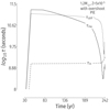 |
Fig. 8. Time evolution of the three timescales, τHe, τdiff, and τH, for the first thermal pulse of the 1.2 M⊙, Z = 5 × 10⁻⁵ star with |fPDCZ| = 0.008 and |fCE| = 0.016. The zero point for time in the x-axis is the point when the PDCZ first appears for this pulse. |
4.2. Comparison with previous works
The mass and metallicity of the star in this work are close to that used in Cristallo et al. (2009) and that of Choplin et al. (2021, 2022). Though, not identical in mass nor in metallicity it is close enough to allow for a comparison. In both cases no overshoot was used at any point in the evolution which is an important difference to our models. All comparisons here will be to our fiducial model unless otherwise specified.
In Cristallo et al. (2009) they simulate a 1.5 M⊙, Z = 5 × 10⁻⁵ star. The PIE and subsequent splitting of the PDCZ occur in the same way in their models as in ours, including the fact that the split happens before the maximum neutron density. The maximum neutron density in their models is however larger at approximately 1 × 1015 cm−3. The split convective zones then never merge again and the upper convective zone merges with the envelope in what they refer to as “deep TDU”. In contrast to our model their model goes on to have many more TPs and many additional TDUs, whereas our models experience at most one post-PIE TDU. This causes more of the material in the lower part of the split PDCZ to nevertheless make its way to the surface of the star than in our model. Again, this occurs because each subsequent PDCZ will overlap with the region where the lower part of the PDCZ was and thus mix the material from the lower part of the PDCZ throughout the intershell. The TDU can then dredge this material up to the surface. One reason for this difference could be the higher mass. Not only is TDU easier at higher masses, the abundance enhancement that occurs is diluted over a larger (in mass) envelope thus reducing the C/O value and in turn leading to a smaller increase in the mass loss rate and a longer lifetime on the AGB. This behavior is seen in Choplin et al. (2022). Another important difference is the different mixing scheme employed by Cristallo et al. (2009). They use a linear mixing scheme instead of our diffusive mixing scheme. With regards to light element nucleosynthesis, they also obtain large amounts of Li enhancement as well as N enhancement.
In the series of papers from the Brussels group they simulate a 1.0 M⊙, Z = 4.3 × 10⁻⁵ star. The largest difference between our models and theirs is that theirs experience the PDCZ split only after the neutron density maximum. In terms of abundances their model post-PIE has 12C/13C = 4.98 in mass as opposed to our value of 6.2 as well as C/O = 3.46 in mass as opposed to our 20.55. The exact value of these ratios ultimately depend on a number of factors including, but not limited to, the competition between the triple-alpha reaction rate, the CNO cycle rates, and the 13C neutron source reaction rate, the ingestion by the PDCZ of material that has been processed by the H shell and thus has CNO-like values for these ratios, the depth at which the PDCZ splits, when during the pulse the PDCZ splits, and the composition of the envelope prior to the PIE. That being said, we can draw some conclusions simply by looking at how the value of these ratios change in the upper part of the split PDCZ after the split. After the PDCZ splits the 12C/13C ratio continues to decrease. This is the result of the combined effect of the continued CNO cycle burning that is still occurring in the convective zone since temperatures there are up to 80 MK and the continued expansion of the upper boundary of the convective zone into regions with lower 12C/13C ratio values. The C/O ratio in the upper part of the PDCZ, however, does not change after the split suggesting that the CNO cycle burning does not have a significant impact on the C/O ratio here. This implies that the C/O ratio is primarily the result of the nucleosynthesis in the lower part of the PDCZ prior to the split. In Figs. 4 and 5 of Choplin et al. (2022) they show which reactions are the most energetic at the base of the PDCZ before the split and each of the 8 reactions shown in these plots alter the C/O ratio. The triple-alpha reaction and the 13C neutron source reaction have the highest rates there and thus are primarily responsible for the final C/O ratio. Therefore, a different temperature stratification in that part of the PDCZ, or different reaction rates for those reactions, or even allowing those reactions to occur over a longer period of time by having the split occur later would all impact the final C/O ratio.
In Choplin et al. (2024) the same 1.0 M⊙, Z = 4.3 × 10⁻⁵ star is run with varying overshoot parameters. Their paper focuses mainly on the impact of overshoot on the heavy element abundances and importantly only calculates the PIEs for these models up until the split point. Nevertheless, there are a few things that can be compared between our study and theirs. First, we also see that the evolution of Nn proceeds more smoothly when overshoot is applied to the PDCZ. Second, the duration of the PIE was also found to decrease with |fPDCZ| in our models. This brings us to the question of the neutron exposure. We find a similar dependence of the neutron exposure on the overshoot of the PDCZ. Namely, that the neutron exposure quickly drops with increasing |fPDCZ|. However, in the models of Choplin et al. (2024) this lower neutron exposure is a result of the shorter PIE with higher PDCZ overshoot values. In our models the lower neutron exposures in models with PDCZ overshoot are to a small extent the result of the shorter PIEs but to a larger extent the result of lesser neutron densities. Furthermore, our neutron densities are systematically lower than theirs which may well be the result of our neutron densities only being estimates due to our network being insufficiently large to follow the detailed nucleosynthesis of the heavier elements. Finally, they find that the overshoot from the base of the CE or from the base of the PDCZ only affect the surface abundances by 0.1 and 0.5 dex, respectively. This is mostly true for our models as well with only Li being more sensitive to the CE overshoot at up to 0.2 dex. Additionally, however, overshoot at the base of the envelope has a non-negligible impact on the neutron exposures (at most around a 75% reduction) and neutron densities (up to 0.8 dex) in our models. The lighter elements are not discussed much in Choplin et al. (2024) but the authors do mention that they systematically under produce the CNO elements whereas in our models the CNO elements match the observations well with C perhaps even being overproduced.
The dependence of the maximum neutron density on the overshoot values in our models is likely due to the manner in which the protons are ingested. It is known that the rate and amount of protons ingested can have an impact of the evolution of the PIE and on the neutron exposures (Sweigart 1973; Malaney 1986; Choplin et al. 2024). Both |fCE| and |fPDCZ| could have an impact on the ingestion of the protons. A high |fCE| results in a H shell that is deeper in the star and thus closer to the base of the PDCZ. A high |fPDCZ| would impact how quickly the PDCZ reaches the H shell among other things. Each effect could impact the rate and total amount of protons ingested during the PIE.
4.3. Comparison with observations
The final surface abundances of our models can also be compared to the growing number of observations of CEMP-r/s stars. Following Karinkuzhi et al. (2021) CEMP-r/s stars are classified as such based on their abundance distribution’s distance to an r-process distribution. All the objects used for comparison in this study are those that were defined as CEMP-r/s from the Karinkuzhi et al. (2021) paper as well as a number of additional objects from Choplin et al. (2021). All objects have [Fe/H] between –2 and –3 and are CEMP-r/s stars based on the Karinkuzhi et al. (2021) classification system. The basic properties of these objects can be seen in Table 2.
The comparisons of the models to the observations can be seen in Figs. 9 and 10. In Fig. 9 there is an additional set of points that are in blue and are the so-called diluted abundances. As previously stated these CEMP-r/s stars owe their peculiar abundance to a mass transfer phase with a companion star which is where the i-process actually occurred. Thus, when comparing abundances one does not compare directly to the abundance of the i-process star model but rather one imagines that material with the same abundances as the surface of the i-process star is mixed or diluted with material that represents the composition of the CEMP-r/s star prior to mass transfer. The easiest assumption to make is that the CEMP-r/s star before mass transfer has the same composition as the initial composition of the i-process star. In that case the abundance of the diluted material can be calculated as
 (8)
(8)
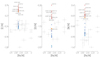 |
Fig. 9. Abundance of [C/H] (top), [O/H] (middle), and [N/H] (bottom) vs. [Fe/H]. The gray points are the observations including errors where available. The red points are the models in Table A.1 while the blue points are the abundances after the dilution factor (f = 0.85) has been applied. The points corresponding to the fiducial model are in orange and light blue, respectively, and marked as a star. Some of the non-diluted points are labeled by the |fPDCZ| and |fCE| values for reference. |
where X* is the abundance of the i-process star, Xinitial is the initial abundance, and f is the dilution factor, a free parameter ranging in value from 0 to 1. The f value used in Fig. 9 is 0.85 which was chosen as it provides a good match to the observations. This high value of f is in line with what is found in Choplin et al. (2021) which they argue is good as it requires less extreme amounts of material to be accreted and a significantly reduced accretion efficiency (see erratum for Choplin et al. 2021). Another paper used this dilution approach in the study of the s-process abundance enhancement in Ba stars and found that for longer period systems the average of the best-fitting f was ∼0.7 while for shorter period systems the ideal f is lower (Cseh et al. 2022). For C, N, and O the diluted material of our models matches well to the observations, though models without overshoot from the PDCZ may have too little O depending on which f is used.
Figure 10 shows abundance ratios plotted against each other. In this case no dilution factor is applied as the dilution would affect all elements equally and thus not affect the element ratios. The results show that our models with no overshoot from the PDCZ, including the fiducial model, are in good agreement and as |fPDCZ| grows the agreement gets worse. Based on this, high overshoot values for the PDCZ are not favored.
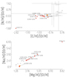 |
Fig. 10. Abundance ratios of [N/H]/[O/H] vs. [C/H]/[O/H] (top) and [Na/H]/[O/H] vs. [Mg/H]/[O/H] (bottom). The gray points are the observations including errors where provided. The red points are the models in Table A.1. The point corresponding to the fiducial model is in orange and marked as a star. Some of the non-diluted points are labeled by the |fPDCZ| and |fCE| values for reference. |
Overall, our models provide a good match to the observations of the absolute abundances when using a large dilution factor. This could be a hint that the magnitude of the enhancement in our models is too large, though the value of the dilution factor is in line with other studies. Regardless, the match to the observations of the abundance ratios is promising.
The magnitude of the individual element enhancements and the element abundance ratios are the product of two different effects. The magnitude of the enhancement is the result of how much of the enriched material is dredged up to the surface. This is dependent not only on the overshoot values but also on the location in the PDCZ where the split occurs. The closer to the bottom of the PDCZ the split occurs the larger the upper part of the split PDCZ is and the more material is brought to the surface when it merges with the envelope. The abundance ratios on the other hand are more dependent on the temperatures at which the burning take place. In the top panel of Fig. 10 the models on the right, closest to the observations, are also those models for which the maximum temperature of the H-burning region during the PIE is smaller. As the models move to lower [C/H]/[O/H] and lower [N/H]/[O/H] this temperature is increasing. Similarly, in the bottom panel of Fig. 10 as the maximum H-burning temperature during the PIE increases the models move further up and to the right in the plot.
As a final point of focus in this section, we discuss Li. Because of the relatively few observations of Li abundance in CEMP-r/s stars a different sample of stars was used than in the previous discussion; these stars are listed in Table 3. All stars are CEMP-r/s stars with [Fe/H] between –2 and –3 (Z between 1.7 × 10⁻⁴ and 1.7 × 10⁻⁵) and observed Li abundances.
Key characteristics of the observed CEMP-r/s stars used in the Li analysis.
As can be seen in Fig. 11 the Li abundances of our models tend to be high even after dilution, though still within observational constraints for the more Li-rich stars in our sample. For consistency the dilution factor was kept the same as before (f = 0.85). Additionally, the models without PDCZ overshoot, including the fiducial model, are more Li-rich than the most Li-rich stars in our sample even after dilution.
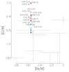 |
Fig. 11. Abundance of [Li/H] vs. [Fe/H]. The plot elements and dilution factor are the same as in Fig. 9. Those observations for which only a maximum Li abundance is provided have a downward facing arrow as an error bar for their Li abundances. All of the non-diluted points are labeled by the |fPDCZ| and |fCE| values for reference. |
5. Conclusions
Using |GARSTEC| we calculated a set of models for a 1.2 M⊙, Z = 5 × 10⁻⁵ ([Fe/H] = −2.56) star with varying overshoot parameters in order to investigate overshoot’s impact on PIEs and the i-process. It was found that models calculated by |GARSTEC|, both with and without overshoot, experience PIEs that generate neutron densities in excess of 1 × 10⁻¹³ cm−3, well within the range needed for the i-process. A fiducial model without overshoot was calculated as a point of comparison for the other models. This model experiences a PIE with very high neutron densities, but it also experiences a splitting of the PDCZ that occurs before the maximum neutron density is reached. The split convective zones never remerge. After the PIE the star goes on to experience three more TPs with the first post-PIE TP being followed by a particularly strong TDU.
Models that included overshoot did differ from the fiducial model in some key ways. Models with overshoot only at the base of the CE had slightly higher final C/O ratios and deeper TDUs during the first post-PIE TP cycle. This may be important for the details of the final surface abundance pattern of the neutron-capture elements, but the affect on the structure and evolution of the star are nominal. The same can not be said of those tracks with overshoot from the PDCZ. While most of these tracks still experience the PDCZ split before the maximum in the neutron density occurs, they exhibit an either partial or permanent remerging of the split PDCZ. This is attributed to the ability of the overshoot region to bridge the gap between the splitting zones for a short time. Additionally, the final C/O ratio is much lower for these tracks as a direct result of the stronger flash and increased temperatures in the He shell which leads to more O and less C being produced. Finally, the neutron exposure and neutron densities show an inverse relationship with |fPDCZ|.
The final surface abundances of these tracks show that the C/O and N/O ratios vary considerably between the models with different amounts of overshoot. Additionally, all models show signs of strong Li enhancement.
As part of the calculation of the fiducial model, testing of temporal and spatial resolution was conducted. This lead to the same conclusion as other studies; namely that with a coarse enough time stepping one can miss the PIE entirely. We then introduced a new timescale argument that can be used to determine if a PIE should occur at a particular pulse or not. The timescales were calculated for a variety of models to show the efficacy of this method.
Finally, our results were compared to those of previous studies as well as to observations of CEMP-r/s stars. The comparison to observations showed that the surface enhancements in our models, particularly those of C and Li, may be too large, though not unrealistic. However, in looking at abundance ratios we see that they do provide a good match to the observations.
Based on the results shown here our recommendation for overshoot parameters is |fPDCZ| = 0.008 and |fCE| = 0.016. This track not only shows good agreement in the final surface abundances of C, N, O, and Li but also has a high neutron exposure. Based on Fig. 10, increasing |fPDCZ| much beyond 0.008 will lead to improper final surface abundances while those models with an |fPDCZ| of zero may have too little O enhancement. This restriction of |fPDCZ| to relatively small values is consistent with the conclusions of Wagstaff et al. (2020) who constrain the overshoot on the AGB of more metal-rich models via comparison to a number of observational constraints. There is more freedom in the choice for |fCE| as it is not well constrained by the data presented in this work.
In the future this study will be expanded to a range of mass and metallicity and will include post-processing calculations for a proper accounting of the nucleosynthesis of these stars.
In this work PIE will be used.
Unless otherwise indicated, this will be the reference for all details of the code.
[X/H] is given by [X/H] = log(X*/H*)−log(X⊙/H⊙).
Acknowledgments
B.R. would like to thank Lionel Siess and Arthur Choplin for their hospitality during a visit as well as for comments, helpful discussions, and certain code comparisons. B.R. would further like to thank Maria Lugaro for her time and support during a visit. Finally, the authors would like to thank the referee for their careful reading of the paper and thoughtful comments that improved the clarity of this work. This research was supported by the Excellence Cluster ORIGINS which is funded by the Deutsche Forschungsgemeinschaft (DFG, German Research Foundation) under Germany’s Excellence Strategy – EXC-2094 – 390783311.
References
- Anders, E. H., & Pedersen, M. G. 2023, Galaxies, 11, 56 [NASA ADS] [CrossRef] [Google Scholar]
- Angulo, C., Arnould, M., Rayet, M., et al. 1999, Nucl. Phys. A, 656, 3 [Google Scholar]
- Aoki, W., Ryan, S. G., Norris, J. E., et al. 2002a, ApJ, 580, 1149 [Google Scholar]
- Aoki, W., Norris, J. E., Ryan, S. G., Beers, T. C., & Ando, H. 2002b, ApJ, 567, 1166 [Google Scholar]
- Aoki, W., Bisterzo, S., Gallino, R., et al. 2006, ApJ, 650, L127 [NASA ADS] [CrossRef] [Google Scholar]
- Aoki, W., Beers, T. C., Christlieb, N., et al. 2007, ApJ, 655, 492 [NASA ADS] [CrossRef] [Google Scholar]
- Aoki, W., Beers, T. C., Sivarani, T., et al. 2008, ApJ, 678, 1351 [Google Scholar]
- Battich, T., Miller Bertolami, M. M., Serenelli, A. M., Justham, S., & Weiss, A. 2023, A&A, 680, L13 [NASA ADS] [CrossRef] [EDP Sciences] [Google Scholar]
- Beers, T. C., & Christlieb, N. 2005, ARA&A, 43, 531 [NASA ADS] [CrossRef] [Google Scholar]
- Bossini, D., Miglio, A., Salaris, M., et al. 2017, MNRAS, 469, 4718 [Google Scholar]
- Brogaard, K., Arentoft, T., Miglio, A., et al. 2023, A&A, 679, A23 [NASA ADS] [CrossRef] [EDP Sciences] [Google Scholar]
- Cameron, A. G. W. 1955, ApJ, 121, 144 [NASA ADS] [CrossRef] [Google Scholar]
- Cameron, A. G. W., & Fowler, W. A. 1971, ApJ, 164, 111 [NASA ADS] [CrossRef] [Google Scholar]
- Campbell, S. W., Lugaro, M., & Karakas, A. I. 2010, A&A, 522, L6 [NASA ADS] [CrossRef] [EDP Sciences] [Google Scholar]
- Choplin, A., Siess, L., & Goriely, S. 2021, A&A, 648, A119 [NASA ADS] [CrossRef] [EDP Sciences] [Google Scholar]
- Choplin, A., Siess, L., & Goriely, S. 2022, A&A, 667, A155 [NASA ADS] [CrossRef] [EDP Sciences] [Google Scholar]
- Choplin, A., Siess, L., Goriely, S., & Martinet, S. 2024, A&A, 684, A206 [NASA ADS] [CrossRef] [EDP Sciences] [Google Scholar]
- Ciani, G. F., Csedreki, L., Rapagnani, D., et al. 2021, Phys. Rev. Lett., 127, 152701 [CrossRef] [PubMed] [Google Scholar]
- Cohen, J. G., Christlieb, N., Qian, Y. Z., & Wasserburg, G. J. 2003, ApJ, 588, 1082 [Google Scholar]
- Cohen, J. G., Christlieb, N., Thompson, I., et al. 2013, ApJ, 778, 56 [Google Scholar]
- Cowan, J. J., & Rose, W. K. 1977, ApJ, 212, 149 [Google Scholar]
- Cristallo, S., Piersanti, L., Straniero, O., et al. 2009, PASA, 26, 139 [Google Scholar]
- Cruz, M. A., Serenelli, A., & Weiss, A. 2013, A&A, 559, A4 [NASA ADS] [CrossRef] [EDP Sciences] [Google Scholar]
- Cseh, B., Világos, B., Roriz, M. P., et al. 2022, A&A, 660, A128 [NASA ADS] [CrossRef] [EDP Sciences] [Google Scholar]
- Cyburt, R. H., Amthor, A. M., Ferguson, R., et al. 2010, ApJS, 189, 240 [NASA ADS] [CrossRef] [Google Scholar]
- Dardelet, L., Ritter, C., Prado, P., et al. 2014, XIII Nuclei in the Cosmos (NIC XIII), 145 [Google Scholar]
- Denissenkov, P. A., Herwig, F., Battino, U., et al. 2017, ApJ, 834, L10 [Google Scholar]
- Denissenkov, P. A., Herwig, F., Woodward, P., et al. 2019, MNRAS, 488, 4258 [Google Scholar]
- Despain, K. H., & Scalo, J. M. 1976, ApJ, 208, 789 [NASA ADS] [CrossRef] [Google Scholar]
- Freytag, B., Ludwig, H. G., & Steffen, M. 1996, A&A, 313, 497 [NASA ADS] [Google Scholar]
- Fujimoto, M. Y. 1977, PASJ, 29, 331 [NASA ADS] [Google Scholar]
- Fujimoto, M. Y., Iben, I., Jr., & Hollowell, D. 1990, ApJ, 349, 580 [CrossRef] [Google Scholar]
- Fujimoto, M. Y., Ikeda, Y., & Iben, I., Jr. 2000, ApJ, 529, L25 [NASA ADS] [CrossRef] [Google Scholar]
- Gallino, R., Arlandini, C., Busso, M., et al. 1998, ApJ, 497, 388 [Google Scholar]
- Goriely, S., Siess, L., & Choplin, A. 2021, A&A, 654, A129 [NASA ADS] [CrossRef] [EDP Sciences] [Google Scholar]
- Grevesse, N., & Sauval, A. J. 1998, Space Sci. Rev., 85, 161 [Google Scholar]
- Hampel, M., Stancliffe, R. J., Lugaro, M., & Meyer, B. S. 2016, ApJ, 831, 171 [Google Scholar]
- Hansen, T., Hansen, C. J., Christlieb, N., et al. 2015, ApJ, 807, 173 [Google Scholar]
- Herwig, F. 2000, A&A, 360, 952 [NASA ADS] [Google Scholar]
- Herwig, F. 2005, ARA&A, 43, 435 [NASA ADS] [CrossRef] [Google Scholar]
- Herwig, F., Pignatari, M., Woodward, P. R., et al. 2011, ApJ, 727, 89 [Google Scholar]
- Iben, I., Jr. 1975, ApJ, 196, 549 [NASA ADS] [CrossRef] [Google Scholar]
- Iben, I., Jr. 1982, ApJ, 260, 821 [CrossRef] [Google Scholar]
- Iglesias, C. A., & Rogers, F. J. 1996, ApJ, 464, 943 [NASA ADS] [CrossRef] [Google Scholar]
- Ivans, I. I., Sneden, C., Gallino, R., et al. 2005, in From Lithium to Uranium: Elemental Tracers of Early Cosmic Evolution, eds. V. Hill, P. Francois, & F. Primas, IAU Symp., 228, 467 [NASA ADS] [Google Scholar]
- Iwamoto, N. 2009, PASA, 26, 145 [NASA ADS] [CrossRef] [Google Scholar]
- Iwamoto, N., Kajino, T., Mathews, G. J., Fujimoto, M. Y., & Aoki, W. 2004, ApJ, 602, 377 [Google Scholar]
- Jaeger, M., Kunz, R., Mayer, A., et al. 2001, Phys. Rev. Lett., 87, 202501 [CrossRef] [PubMed] [Google Scholar]
- Jones, S., Ritter, C., Herwig, F., et al. 2016, MNRAS, 455, 3848 [Google Scholar]
- Jonsell, K., Barklem, P. S., Gustafsson, B., et al. 2006, A&A, 451, 651 [NASA ADS] [CrossRef] [EDP Sciences] [Google Scholar]
- Karakas, A. I., & Lattanzio, J. C. 2014, PASA, 31, e030 [NASA ADS] [CrossRef] [Google Scholar]
- Karinkuzhi, D., Van Eck, S., Goriely, S., et al. 2021, A&A, 645, A61 [EDP Sciences] [Google Scholar]
- Kippenhahn, R., Weigert, A., & Weiss, A. 2013, in Stellar Structure and Evolution, (Heidelberg: Springer Berlin) [Google Scholar]
- Kitsikis, A. 2008, Ph.D. Thesis, Ludwig-Maximilians-Universität München, Germany [Google Scholar]
- Kitsikis, A., & Weiss, A. 2007, in Why Galaxies Care about AGB Stars: Their Importance as Actors and Probes, eds. F. Kerschbaum, C. Charbonnel, & R. F. Wing, ASP Conf. Ser., 378, 99 [NASA ADS] [Google Scholar]
- Kitsikis, A., & Weiss, A. 2008, in Mass Loss from Stars and the Evolution of Stellar Clusters, eds. A. de Koter, L. J. Smith, & L. B. F. M. Waters, ASP Conf. Ser., 388, 183 [NASA ADS] [Google Scholar]
- Kunz, R., Fey, M., Jaeger, M., et al. 2002, ApJ, 567, 643 [CrossRef] [Google Scholar]
- Lau, H. H. B., Stancliffe, R. J., & Tout, C. A. 2009, MNRAS, 396, 1046 [CrossRef] [Google Scholar]
- Lau, H. H. B., Gil-Pons, P., Doherty, C., & Lattanzio, J. 2012, A&A, 542, A1 [Google Scholar]
- Lugaro, M., Herwig, F., Lattanzio, J. C., Gallino, R., & Straniero, O. 2003, ApJ, 586, 1305 [NASA ADS] [CrossRef] [Google Scholar]
- Lugaro, M., Karakas, A. I., Stancliffe, R. J., & Rijs, C. 2012, ApJ, 747, 2 [Google Scholar]
- Maeder, A., & Meynet, G. 1991, A&AS, 89, 451 [NASA ADS] [CrossRef] [Google Scholar]
- Magic, Z., Serenelli, A., Weiss, A., & Chaboyer, B. 2010, ApJ, 718, 1378 [NASA ADS] [CrossRef] [Google Scholar]
- Malaney, R. A. 1986, MNRAS, 223, 709 [NASA ADS] [CrossRef] [Google Scholar]
- Marigo, P. 2002, A&A, 387, 507 [NASA ADS] [CrossRef] [EDP Sciences] [Google Scholar]
- Masseron, T., Johnson, J. A., Lucatello, S., et al. 2012, ApJ, 751, 14 [NASA ADS] [CrossRef] [Google Scholar]
- Miller Bertolami, M. M. 2016, A&A, 588, A25 [NASA ADS] [CrossRef] [EDP Sciences] [Google Scholar]
- Mishenina, T., Pignatari, M., Carraro, G., et al. 2015, MNRAS, 446, 3651 [Google Scholar]
- Ostlie, D. A., & Cox, A. N. 1986, ApJ, 311, 864 [NASA ADS] [CrossRef] [Google Scholar]
- Placco, V. M., Frebel, A., Beers, T. C., et al. 2013, ApJ, 770, 104 [Google Scholar]
- Reimers, D. 1975, MSRSL, 8, 369 [NASA ADS] [Google Scholar]
- Roederer, I. U., Preston, G. W., Thompson, I. B., et al. 2014, AJ, 147, 136 [Google Scholar]
- Rogers, F. J., & Nayfonov, A. 2002, ApJ, 576, 1064 [Google Scholar]
- Rossi, S., Beers, T. C., & Sneden, C. 1999, in The Third Stromlo Symposium: The Galactic Halo, eds. B. K. Gibson, R. S. Axelrod, & M. E. Putman, ASP Conf. Ser., 165, 264 [NASA ADS] [Google Scholar]
- Sackmann, I. J. 1977, ApJ, 212, 159 [CrossRef] [Google Scholar]
- Schwarzschild, K. 1906, Nachrichten von der Königlichen Gesellschaft der Wissenschaften zu Göttingen. Math.-phys. Klasse, 195, 41 [Google Scholar]
- Sivarani, T., Bonifacio, P., Molaro, P., et al. 2004, A&A, 413, 1073 [NASA ADS] [CrossRef] [EDP Sciences] [Google Scholar]
- Stein, R. F. 1966, Stellar Evolution: A Survey with Analytic Models (Plenum Press), 3 [Google Scholar]
- Stothers, R. B., & Chin, C.-W. 1992, ApJ, 390, 136 [NASA ADS] [CrossRef] [Google Scholar]
- Straniero, O., Gallino, R., Busso, M., et al. 1995, ApJ, 440, L85 [NASA ADS] [CrossRef] [Google Scholar]
- Suda, T., & Fujimoto, M. Y. 2010, MNRAS, 405, 177 [NASA ADS] [Google Scholar]
- Suda, T., Yamada, S., Katsuta, Y., et al. 2011, MNRAS, 412, 843 [NASA ADS] [Google Scholar]
- Sugimoto, D. 1970, Prog. Theor. Phys., 44, 375 [CrossRef] [Google Scholar]
- Susmitha, A., Ojha, D. K., Sivarani, T., et al. 2021, MNRAS, 506, 1962 [NASA ADS] [CrossRef] [Google Scholar]
- Sweigart, A. V. 1973, A&A, 24, 459 [NASA ADS] [Google Scholar]
- Thielemann, F. K., Arcones, A., Käppeli, R., et al. 2011, Prog. Part. Nucl. Phys., 66, 346 [NASA ADS] [CrossRef] [Google Scholar]
- Tomkin, J., Lambert, D. L., Edvardsson, B., Gustafsson, B., & Nissen, P. E. 1989, A&A, 219, L15 [NASA ADS] [Google Scholar]
- van Loon, J. T., Cioni, M.-R. L., Zijlstra, A. A., & Loup, C. 2005, A&A, 438, 273 [NASA ADS] [CrossRef] [EDP Sciences] [Google Scholar]
- Ventura, P., García-Hernández, D. A., Dell’Agli, F., et al. 2016, ApJ, 831, L17 [Google Scholar]
- Wachter, A., Schröder, K.-P., Winters, J. M., Arndt, T. U., & Sedlmayr, E. 2002, A&A, 384, 452 [NASA ADS] [CrossRef] [EDP Sciences] [Google Scholar]
- Wagstaff, G. 2018, Ph.D. Thesis, Ludwig-Maximilians-Universität München, Germany [Google Scholar]
- Wagstaff, G., Miller Bertolami, M. M., & Weiss, A. 2020, MNRAS, 493, 4748 [Google Scholar]
- Weiss, A., & Ferguson, J. W. 2009, A&A, 508, 1343 [NASA ADS] [CrossRef] [EDP Sciences] [Google Scholar]
- Weiss, A., & Schlattl, H. 2008, Ap&SS, 316, 99 [CrossRef] [Google Scholar]
- Wood, P. R., & Faulkner, D. J. 1986, ApJ, 307, 659 [NASA ADS] [CrossRef] [Google Scholar]
- Xu, Y., Takahashi, K., Goriely, S., et al. 2013, Nucl. Phys. A, 918, 61 [Google Scholar]
- Zhang, L., Karlsson, T., Christlieb, N., et al. 2011, A&A, 528, A92 [NASA ADS] [CrossRef] [EDP Sciences] [Google Scholar]
Appendix A: Additional Table
Table A.1 shows the final surface abundances of all the models run in this study in both mass fraction and [X/H].
Final surface abundances of the i-process tracks. All abundances are given as the decimal log of the mass fraction followed by the [X/H] in parentheses.
All Tables
Selected key results of the stellar evolution models for all the tracks discussed in this section.
Final surface abundances of the i-process tracks. All abundances are given as the decimal log of the mass fraction followed by the [X/H] in parentheses.
All Figures
|
Fig. 1. Depiction of the nuclear network of |GARSTEC| in this work. The blue squares represent those isotopes that are in the nuclear network in the main branch of |GARSTEC|. Red isotopes are ones that have been added to the network in the AGB branch. As is standard practice we have included both the ground state and the isomeric state of 26Al. The main neutron source reactions and the primary neutron poison reaction are marked with arrows. |
| In the text | |
|
Fig. 2. Time evolution of the H luminosity (in blue) and the He luminosity (in orange) of the fiducial model during the PIE. |
| In the text | |
|
Fig. 3. Kippenhahn diagrams showing the structure of the fiducial model (top) and the maximum neutron density (bottom). Time is shown as model number on the lower x-axis and as time in days relative to the maximum neutron density in the upper x-axis. In the Kippenhahn diagram the top and bottom of the H shell is denoted by the solid blue lines with the dotted blue line following the point of maximum H burning in the shell. The top and the bottom of the He shell is denoted by the solid orange lines with the orange dashed line following the point of maximum He burning in the shell. Formally Convective regions are shown in gray. |
| In the text | |
|
Fig. 4. Kippenhahn diagrams (see Fig. 3 for an explanation of the plot elements) of a PIE. Top panel: the |fPDCZ| = 0.016, |fCE| = 0.016 track experiences a partial remerging that occurs around model 23 800. Additionally, one can see the dredge-up-like event that happens when the upper part of the split PDCZ descends into the region below the split point. Bottom panel: the |fPDCZ| = 0.016, |fCE| = 0.016 track without the geometrical cut-off to the overshoot experiences a permanent remerging. |
| In the text | |
|
Fig. 5. Time evolution of the surface abundances (in mass fraction) of certain elements for the |fPDCZ| = 0.008, |fCE| = 0.000 track. |
| In the text | |
|
Fig. 6. Time evolution of the three timescales, τHe, τdiff, and τH, for the third thermal pulse in a 3 M⊙, solar metallicity model (top) and a 1.2 M⊙, Z = 5 × 10⁻⁴ model (bottom). No PIEs are expected for stars with these parameters. The zero point for time in the x-axis is the point when the PDCZ first appears for this pulse. |
| In the text | |
|
Fig. 7. Time evolution of the three timescales, τHe, τdiff, and τH, for the third thermal pulse of the 1.2 M⊙, Z = 5 × 10⁻⁵ model with poor temporal resolution (top) and the fiducial model (bottom). In the upper panel the code has missed the PIE due to poor time stepping while in the lower panel the PIE was resolved. The zero point for time in the x-axis is the point when the PDCZ first appears for this pulse. |
| In the text | |
|
Fig. 8. Time evolution of the three timescales, τHe, τdiff, and τH, for the first thermal pulse of the 1.2 M⊙, Z = 5 × 10⁻⁵ star with |fPDCZ| = 0.008 and |fCE| = 0.016. The zero point for time in the x-axis is the point when the PDCZ first appears for this pulse. |
| In the text | |
|
Fig. 9. Abundance of [C/H] (top), [O/H] (middle), and [N/H] (bottom) vs. [Fe/H]. The gray points are the observations including errors where available. The red points are the models in Table A.1 while the blue points are the abundances after the dilution factor (f = 0.85) has been applied. The points corresponding to the fiducial model are in orange and light blue, respectively, and marked as a star. Some of the non-diluted points are labeled by the |fPDCZ| and |fCE| values for reference. |
| In the text | |
|
Fig. 10. Abundance ratios of [N/H]/[O/H] vs. [C/H]/[O/H] (top) and [Na/H]/[O/H] vs. [Mg/H]/[O/H] (bottom). The gray points are the observations including errors where provided. The red points are the models in Table A.1. The point corresponding to the fiducial model is in orange and marked as a star. Some of the non-diluted points are labeled by the |fPDCZ| and |fCE| values for reference. |
| In the text | |
|
Fig. 11. Abundance of [Li/H] vs. [Fe/H]. The plot elements and dilution factor are the same as in Fig. 9. Those observations for which only a maximum Li abundance is provided have a downward facing arrow as an error bar for their Li abundances. All of the non-diluted points are labeled by the |fPDCZ| and |fCE| values for reference. |
| In the text | |
Current usage metrics show cumulative count of Article Views (full-text article views including HTML views, PDF and ePub downloads, according to the available data) and Abstracts Views on Vision4Press platform.
Data correspond to usage on the plateform after 2015. The current usage metrics is available 48-96 hours after online publication and is updated daily on week days.
Initial download of the metrics may take a while.