| Issue |
A&A
Volume 684, April 2024
|
|
|---|---|---|
| Article Number | A34 | |
| Number of page(s) | 24 | |
| Section | Interstellar and circumstellar matter | |
| DOI | https://doi.org/10.1051/0004-6361/202348391 | |
| Published online | 03 April 2024 | |
THEMIS 2.0: A self-consistent model for dust extinction, emission, and polarisation
1
Université Paris-Saclay, CNRS, Institut d'Astrophysique Spatiale,
91405
Orsay,
France
e-mail: This email address is being protected from spambots. You need JavaScript enabled to view it.
2
IRAP, CNRS, Université de Toulouse,
9 avenue du Colonel Roche,
31028
Toulouse Cedex 4,
France
3
LUPM, Université de Montpellier, CNRS/IN2P3,
CC 72, Place Eugène Bataillon,
34095
Montpellier Cedex 5,
France
4
Space Telescope Science Institute,
3700 San Martin Drive,
Baltimore,
MD
21218,
USA
5
AIM, CEA, CNRS, Université Paris-Saclay, Université Paris Diderot,
Sorbonne Paris Cité,
91191
Gif-sur-Yvette,
France
6
National Chung Hsing University,
145 Xingda Rd., South Dist.,
Taichung City
402,
Taiwan
Received:
26
October
2023
Accepted:
10
January
2024
Abstract
Context. Recent observational constraints in emission, extinction, and polarisation have at least partially invalidated most of the astronomical standard grain models for the diffuse interstellar medium. Moreover, laboratory measurements on interstellar silicate analogues have shown quite significant differences with the optical properties used in these standard models.
Aims. To address these issues, our objective is twofold: (i) to update the optical properties of silicates and (ii) to develop The Heterogeneous dust Evolution Model for Interstellar Solids (THEMIS) to allow the calculation of polarised extinction and emission.
Methods. Based on optical constants measured in the laboratory from 5 µm to 1 mm for amorphous silicates and on observational constraints in mid-IR extinction and X-ray scattering, we defined new optical constants for the THEMIS silicates. Absorption and scattering efficiencies for spheroidal grains using these properties were subsequently derived with the discrete dipole approximation.
Results. These new optical properties make it possible to explain the dust emission and extinction, both total and polarised. It is noteworthy that the model is not yet pushed to its limits since it does not require the perfect alignment of all grains to explain the observations and it therefore has the potential to accommodate the highest polarisation levels inferred from extinction measurements. Moreover, the dispersion of the optical properties of the different silicates measured in the laboratory naturally explain the variations in both the total and polarised emission and extinction observed in the diffuse interstellar medium.
Conclusions. A single, invariant model calibrated on one single set of observations is obsolete for explaining contemporary observations. We are proposing a completely flexible dust model based entirely on laboratory measurements that has the potential to make major advances in understanding the exact nature of interstellar grains and how they evolve as a function of their radiative and dynamic environment. Even if challenging, this is also relevant for future cosmic microwave background (CMB) missions that will aim to perform precise measurements of the CMB spectral distortions and polarisation.
Key words: polarization / dust, extinction / ISM: general / infrared: ISM / submillimeter: ISM
© The Authors 2024
 Open Access article, published by EDP Sciences, under the terms of the Creative Commons Attribution License (https://creativecommons.org/licenses/by/4.0), which permits unrestricted use, distribution, and reproduction in any medium, provided the original work is properly cited.
This article is published in open access under the Subscribe to Open model. This email address is being protected from spambots. You need JavaScript enabled to view it. to support open access publication.
1 Introduction
Detailed knowledge of cosmic dust is crucial for understanding our Universe. It is almost impossible to avoid its effects and we should therefore never underestimate its impact on astronomical observations. Undoubtedly, the thermal emission from interstellar dust is prominent in all observations over the IR to sub-millimetre electromagnetic spectrum. The extinction of starlight is dominated by dust at all galaxy scales. Dust is therefore one of the best tracers of the processes that govern the evolution of cosmic matter in galaxies near and far, from their most diffuse interstellar clouds to the densest regions where stars and planets form. Yet dust is far from being just a tracer, but it is perhaps the major actor in the evolution of matter within the cosmos. For example, the dust opacity is a fundamental parameter for star formation as it determines whether a medium is optically thin or thick and hence how much of the local radiation field can be radiated away, which strongly affects the collapse process leading to new stars. Dust also heats the gas through the photoelectric effect and cools it through gas-grain collisions. It is thus a key player in determining the dynamics of the interstellar medium (ISM) through its interactions with the radiation field and with the gas. Dust is responsible for the diverse chemical complexity seen within galaxies. Its surfaces provide the sites for many chemical reactions that cannot occur in the gas phase, including the formation of H2, and because it is very efficient at absorbing bond-dissociating UV photons it then protects those same molecules from destruction. Many of the most complex molecules, such as alcohols and sugars, exist only because they are formed in the ice layers that coat dust grains in dense star and planet-forming clouds. Further, ISM grains are the very precursors of the solid matter that makes the planets. All of the above processes depend on the exact grain size, structure, composition, and mass; and there is still a gap in our knowledge of these fundamental dust properties. Both the latest observations and laboratory measurements have cast doubt on the validity of the standard grain models for the diffuse ISM which we now consider in some detail.
From an observational point of view, several points are of concern. First of all, the silicate mid-IR vibrational bands are less prominent over the continuum extinction (e.g. Gordon et al. 2021) than those predicted by standard models (e.g. Désert et al. 1990; Draine & Li 2007; Compiègne et al. 2011; Jones et al. 2013; Guillet et al. 2018), with most of them using optical properties derived from the astrosilicates defined by Draine & Lee (1984). Second, the Planck high frequency instrument (Planck-HFI) data revealed a number of inconsistencies between the model predictions for emission and extinction. This applies to both polarised and unpolarised extinction-to-emission ratios, with the deviation between observations and models being of the order of a factor of 2 to 3 (Fanciullo et al. 2015; Planck Collaboration Int. XXI 2015; Planck Collaboration Int. XXIX 2016). This second point is particularly problematic since it is directly related to the estimation of the mass of the ISM structures. Third, there is increasing evidence of variations in the grain properties in the diffuse ISM. Depending on the observed line of sight, the extinction curve has been shown to vary from the UV/optical (e.g. Gordon et al. 2009; Fitzpatrick et al. 2019; Massa et al. 2020) to the near-IR (e.g. Nishiyama et al. 2006, 2009; Decleir et al. 2022) and the mid-IR (e.g. Gordon et al. 2021). Regarding the dust emission, the Planck Collaboration began by showing that the grain sub-millimetre opacity varies on particularly tenuous lines of sight (NH < 3 × 10²⁰ H cm−2, Planck Collaboration XI 2014). This pioneering study was followed by others pointing to variations in opacity in a variety of ways (Reach et al. 2015, 2017) and showing that it was not accompanied by a significant change in the E(B − V)/NH ratio (Nguyen et al. 2018; Murray et al. 2018). Moreover, the gas-to-dust mass ratio, which had been considered constant or even canonical until recently, varies from 20 to 60% in relation to the historical measurement of Bohlin et al. (1978), depending on the line of sight (e.g. Liszt 2014; Planck Collaboration XI 2014; Lenz et al. 2017; Murray et al. 2018; Nguyen et al. 2018; Remy et al. 2018; Van De Putte et al. 2023). These variations are also corroborated by the spectro-polarimetric study led by Siebenmorgen et al. (2018). All of these points lead to a fundamental problem with the dust models and not just to a marginal adjustment. The logical conclusion of this inventory is that there is a need to redefine the optical properties of the silicates responsible for the mid-IR extinction bands and a priori of a large part of the polarised and non-polarised thermal emissions from the far-IR to sub-millimetre. There are two ways of solving this problem: to create an empirical model from fitting of astronomical observations as performed by Hensley & Draine (2023)1 or to start from laboratory measurements on interstellar grain analogues and check their agreement with the observations as in Siebenmorgen (2023). Both approaches are useful; however, in the logic of our previous work (Jones et al. 2017, and citations therein) and in order to be able to characterise the chemical composition of the grains as well as possible and thus all of their physical, chemical, and dynamical properties, we followed the experimental rather than the empirical route.
The laboratory measurements performed by Demyk et al. (2017) are in this sense of paramount importance. They measured the mass absorption coefficients (MACs) of amorphous Mg-rich glassy silicates, which are expected to be good analogues of diffuse ISM solid matter, between 5 µm and 1 mm. This was the first study to measure MACs of amorphous silicates over such a wide wavelength range, a particularly important point being that previous studies did not cover the vibrational bands at 9.7 and 18 µm (Agladze et al. 1996; Mennella et al. 1998; Boudet et al. 2005; Coupeaud et al. 2011). Many of their results differ significantly from the silicates used in the standard models and are consistent with the direction needed to explain the observations: (i) the mid-IR vibrational bands are wider and less prominent with respect to the continuum; (ii) the far-IR to sub-millimetre opacity is higher, as well as wavelength and temperature dependent; and (iii) both opacity and bands are dependent on the chemical composition and structure at the nano-scale of the silicate samples. The optical constants corresponding to these laboratory measurements are now available (Demyk et al. 2022) and our goal is to update the silicate component of our grain model THEMIS2 (The Heterogeneous dust Evolution Model for Interstellar Solids, Jones et al. 2017, and references therein). At the same time, we have moved from spherical to non-spherical grains to allow the calculation of polarisation with this new version of the model, referred to as THEMIS 2.0 afterwards. Solutions to the observational problems raised above have already been proposed by Siebenmorgen (2023) and Hensley & Draine (2023), but our aim is to develop a model that will explain not only the ‘average values’ observed in the diffuse ISM but also their dispersion.
This paper is organised as follows. Section 2 details the new optical constants used for the THEMIS 2.0 silicate component. The methodology of the optical property calculations is described in Sect. 3. Section 4 then presents the variations in the optical properties depending on the grain shapes and sizes. The observational constraints are discussed in Sect. 5 and the THEMIS 2.0 model is subsequently defined in Sect. 6. Section 7 finally summarises our results.
2 THEMIS 2.0 grain chemical compositions
Our starting point is the original version of THEMIS (Jones et al. 2013, 2017; Köhler et al. 2014) in which the grains consist of (sub-)nanometric aromatic-rich a-C carbon grains (0.4 ⩽ a ⩽ 20 nm), larger amorphous carbonaceous grains with an H-rich a-C:H core and a 20 nm-thick aromatic-rich a-C mantle and amorphous Mg-rich silicates with metallic iron and iron sulphide nano-inclusions coated with a 5 nm-thick aromatic-rich a-C carbon mantle3. For the large amorphous carbonaceous grains, the core material is taken to be that typical of the aliphatic-rich, wide band gap, material formed around C-rich evolved stars (e.g. Goto et al. 2000, 2007), while the outer mantle is assumed to have been UV photo-processed in the low density ISM (see Jones 2016, for a more comprehensive explanation). For the amorphous silicate component, THEMIS consists of two chemical compositions: one with a stoichiometry similar to that of enstatite and one to that of forsterite4 (Scott & Duley 1996), with both optical constants quite similar to those of the ‘astrosilicates’ defined by Draine & Lee (1984) for λ ≳ 18 µm. As stated in Sect. 1, the complex refractive index ordinarily assumed for the silicate grains can no longer be considered as the most reliable data set and needs to be replaced by the more consistent measurements performed by Demyk et al. (2017).
2.1 Silicate grains
Demyk et al. (2017) performed measurements on interstellar silicate analogues from the mid-IR to sub-millimetre at 10, 100, 200, and 300 K and subsequently derived the associated complex refractive indices (m = n + ik) as described in Demyk et al. (2022). The analogues were amorphous Mg-rich glassy silicates with the stoichiometry of forsterite (X35 sample in Demyk et al. 2017) and enstatite (X50a and X50b samples). A third sample had a stoichiometry in-between forsterite and enstatite (X40 sample). For clarity and also because it was measured only below λFIR = 500 µm, we choose to discard this sample and rather mix the X35 and X50 samples (see Sect. 2.1.2). The X50a and X50b samples were measured up to λFIR = 0.75 and 1 mm, respectively. Above these threshold values, Demyk et al. (2022) extrapolated the imaginary part of the refractive index and computed its real part according to the Kramers-Kronig relations. The optical constants used in THEMIS 2.0 are those measured at 10 K, the temperature closest to that expected in the diffuse ISM, and it should be noted that Demyk et al. (2017) found no significant variation up to 30 K.
As stated later in Sect. 3, computing the optical properties of core-mantle spheroidal grains is an enormous time-consuming process. This means that it is impossible to test all of the silicate chemical composition combinations in the spheroidal case. A first step in the definition of THEMIS 2.0 is therefore to constrain a plausible silicate chemical composition based on previous studies.
2.1.1 Observational constraints for silicate composition
The majority of the silicates in the diffuse ISM appear to be amorphous (e.g. Kemper et al. 2004; Zeegers et al. 2019), which makes it difficult to characterise their chemical composition. Indeed, contrary to crystalline solids, the 9.7 and 18 µm absorption bands of amorphous silicates are broad and featureless. A second issue concerns the nature of the iron within the grains – in the matrix or in metallic form.
Several studies have compared the mid-IR silicate bands measured in the ISM to those measured on analogues in the laboratory. Although the proportions vary depending on the line of sight considered, most of these studies concluded that the composition is a mixture of olivine and pyroxene stoichiome-try mineralogies (e.g. Chiar & Tielens 2006; van Breemen et al. 2011). Observing the Galactic Centre in the 9.7 µm feature, Kemper et al. (2004) pointed towards a predominance of olivine over pyroxene in proportions of ~85 to 15%. Combining both features at 9.7 and 18 µm, Min et al. (2007) further showed that interstellar silicates have to be highly Mg-rich (Mg/(Mg+Fe) > 0.9) thus leading to the conclusion that iron is incorporated in silicates in the form of metallic inclusions rather than in the matrix. This is consistent with two laboratory studies. The first showed that amorphous Fe-rich silicates that are annealed in the presence of carbon leads to the reduction of the iron and the formation of Fe nano-particles embedded within a matrix of Mg-rich amorphous silicate (Davoisne et al. 2006; Djouadi et al. 2007). The second found that H+ irradiation of amorphous silicates with iron in the matrix leads to selective oxygen sputtering and thus again to the reduction of Fe2+ to metallic Fe (Jäger et al. 2016).
This is also confirmed by observations of dust X-ray absorption and scattering at the Si, Mg, O, and Fe K-edges. Modelling of these data with silicate laboratory analogue optical properties lead to the conclusions that: (i) the Si, Mg, and O K-edge spectral shapes exhibit a major contribution from olivine and pyroxene type silicates (Costantini et al. 2005; Zeegers et al. 2017); (ii) the Fe K-edge structure implies Mg-rich silicates with metallic iron and troilite (FeS) inclusions to be dominant (Xiang et al. 2011; Costantini et al. 2012). Regarding the relative contributions of olivine and pyroxene, two recent X-ray studies concluded that olivine are dominant over pyroxene with proportions of up to ~70 to 30% (Rogantini et al. 2019) and ~80 to 20% (Zeegers et al. 2019). This result is in agreement with analyses of pre-solar silicates (Hoppe et al. 2018, 2022). These proportions may however vary depending on local environment (Demyk et al. 2001) and even be reversed (Psaradaki et al. 2023).
2.1.2 Silicate refractive index
Even if there are still some remaining discrepancies concerning the exact silicate composition and the nature of iron in dust, previous studies seem to indicate that silicates are mostly amorphous Mg-rich with metallic Fe and possibly FeS inclusions5, with the majority of them belonging to the olivine mineralogical family and the others to the pyroxene family.
Demyk et al. (2022) determined the refractive indices of the Mg-rich end members of the amorphous silicates with sto-ichiometries typical of olivine and pyroxene series, forsterite and enstatite, respectively. They considered two samples with the composition of enstatite, X50a and X50b (see Fig. 1). The main differences are in the far-IR and sub-millimetre range for the imaginary part of the refractive index. Beyond the band at 18 µm, the X50a sample shows a much steeper decay than X50b followed by a flattening for λ ≳ 700 µm. Sample X50b does not show a break in the slope. We also note that the band at 10 µm is more contrasted for X50b than X50a. In the following and to test the influence of the choice of the initial laboratory analogue sample, we consider three possible compositions for the silicates. In the first case, we model silicates as being made up of 80% X35 forsterite sample and 20% enstatite, half of which consists of the X50a sample and half of the X50b sample (see Table 1 and Fig. 1). In the second (third) [fourth] case, silicates consist of 70% (50%) [30%] X35 forsterite and 30% (50%) [70%] X50b enstatite. In the fifth (sixth) [seventh] case, silicates consist of 70% (50%) [30%] X35 forsterite and 30% (50%) [70%] X50a enstatite. We use the Bruggeman effective medium theory to derive the refractive index of such silicate mixtures (Bohren & Huffman 1983). Then, true to the original concept of THEMIS, we use the Maxwell Garnett mixing rule to derive the refractive index of Fe/FeS nano-inclusions: Fe and FeS (Ordal et al. 1985, 1988; Pollack et al. 1994) occupy 70 and 30% of the volume of the inclusions, respectively (Köhler et al. 2014). The Maxwell Garnett rule is then used to derive the refractive index of a mixture 90% amorphous silicate plus 10% Fe/FeS inclusions. These optical constants, presented in Fig. 1, are those of the materials called ‘aSil-n’ afterwards (n = 1 to 7) for cases 1 to 7 silicate mixtures, respectively. For the material mixtures containing the X50b sample, the main difference between the three mixtures is an increase in the imaginary part of the spectral index in the sub-millimetre range by a factor of about 1.5 (2.2) [2.9] when moving from aSil-1 to aSil-2 (aSil-3) [aSil-4]. This increase will be reflected in the emissivity of the grains, as will the variations in spectral index. The material mixtures containing the X50a sample present a major break in the slope around 600 µm, the severity of this break being dependent on the X35-to-X50a ratio. The different silicate mixtures are summarised in Table 1. For the sake of comparison, we also perform calculations for the original THEMIS optical constants using a 50%-50% mixture of the amorphous silicates with the normative compositions of forsterite and enstatite as defined in Köhler et al. (2014).
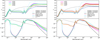 |
Fig. 1 Complex refractive indices, m = n + ik, of the silicate materials. Top: real part. Bottom: imaginary part. Left: complex refractive indices for the calculation of the silicate grain optical properties. Demyk et al. (2017) silicate samples measured at 10 K are shown: forsterite X35 sample (black), enstatite X50a sample (light pink), enstatite X50b sample (light blue) along with the aSil-1, aSil-2, aSil-3, and aSil-4 mixtures as pink, blue, green, and yellow thick lines, respectively (see Sect. 2.1.2 and Table 1 for details). We note that 10% of the silicate volume is occupied by metallic nano-inclusions of Fe and FeS (70% and 30% of the total volume of the inclusions, respectively), hence the increase in the visible to mid-IR imaginary part of the refractive index. For comparison, the optical constants of the two silicate materials used in the original THEMIS are shown with dotted lines. The optical constants used for the 5 nm-thick aromatic-rich carbon mantles, a-C2.5nm, are also plotted (grey, see Sect. 2.2 for details). Right: same for the aSil-5, a-Sil-6, and aSil-7 mixtures as red, brown, and orange thick lines, respectively. |
Silicate core compositions with corresponding line colours in the figures.
2.2 Carbonaceous grains
For the semi-conducting hydrocarbon grains and mantles, we do not modify the optical constants already defined in the original THEMIS framework (Jones 2012a,b,c). However, these being grain size- and hydrogen content-dependent, a size and a band gap have to be chosen in order to define the carbonaceous grain optical properties. For the smallest aromatic-rich a-C grains with 0.4 ⩽ a ⩽ 20 nm, we keep the definition given by Jones et al. (2013) with Eg = 0.1 eV ~4.3XH (see Tamor & Wu 1990).
For the larger grains, we depart from the original THEMIS model. For the cores, we keep the original definition of THEMIS by using the actual aliphatic-rich core size to define its optical constants and a band gap of Eg = 2.5 eV. For the mantles, the original definition corresponds to a perfectly homogeneous 20 nm-thick mantle having a band gap of Eg = 0.1 eV and an equivalent radius equal to half the mantle thickness, 10 nm (called 'characteristic size' afterwards and by definition always smaller than or equal to half the mantle thickness). Since the choice of this characteristic size completely determines the emis-sivity and spectral index in the far-IR and sub-millimetre range, we test several characteristic sizes for the mantle: 2.5, 4, 5, 6, and 10 nm but keep Eg = 0.1 eV and the mantle thickness equal to 20 nm. Schematically, the smallest characteristic size reflects the case where the 20 nm-thick mantle comes mainly from the accretion of aromatic-rich small nano-grains and the largest characteristic size where the 20 nm-thick mantle comes from the aromatisation by stellar UV photons of a parent aliphatic grain in an isotropic and homogeneous way (Jones et al. 2013). In the following, the different carbonaceous mantle types are labelled a-C2.5nm, a-C4nm, a-C5nm, a-C6nm, and a-C10nm for increasing characteristic size. We insist that only the characteristic size describing the mantle formation varies whereas the mantle thickness is fixed at 20 nm. Figure 2 shows that, at long wavelengths, the refractive index increases with characteristic size – leading to stronger emissivities – while the spectral index of its imaginary part decreases.
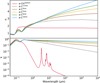 |
Fig. 2 Complex refractive indices, m = n + ik, for the calculation of the carbonaceous grain optical properties with those used for the mantle in grey (2.5 nm a-C), brown (4 nm a-C), orange (5 nm a-C), green (6 nm a-C), and blue (10 nm a-C) and the example of a 100 nm a-CH core in red. Top: real part. Bottom: imaginary part. |
3 Methodology of the optical property calculation
In contrast to total emission and extinction, the dust polarised emission and extinction depend not only on its optical properties, size and shape, but also on the efficiency of its alignment with the local magnetic field and on the orientation of the latter with respect to the line of sight. In this section, we describe the methodology of our calculations for the orientated optical properties (Sect. 3.2) which depend on the way the polarised emission and extinction are computed (Sect. 3.1).
3.1 Maximum polarisation fraction for spheroids
The simplest and most commonly used grain shape in diffuse ISM models is the spheroid (e.g. Lee & Draine 1985; Draine & Fraisse 2009; Siebenmorgen et al. 2014; Voshchinnikov et al. 2016; Guillet et al. 2018, among others), which is obtained by the rotation of an ellipse along one of its main axes. If the rotation is made around the short axis, we refer to it as an oblate grain and if it is around the long axis, as a prolate grain. Calling a the semi-major axis of revolution and b the two other semi-major axes, the ratio b/a is greater than one for oblates and smaller than one for prolates. The effective radius of the sphere of the same volume is then aeff = (ab2)1/3. In the following, the total and polarised emissions and extinctions are calculated with the DustEM6 numerical tool (Compiègne et al. 2011), following the formalism detailed in Guillet et al. (2018), itself based on the approaches of Hong & Greenberg (1980) and Das et al. (2010), that we only briefly summarise below.
For the grains producing the polarised extinction and emission, that is those aligned with the magnetic field, DustEM needs absorption and scattering efficiencies for two orientations of the E component of an incident electromagnetic wave: (i)  with E parallel to the projection of the magnetic field onto the plane of the sky and (ii)
  with E perpendicular to it. Here we only seek to calculate the maximum in polarised extinction and emission and therefore assume that the grains are in perfect spinning alignment, no precession or nutation of the grain spin axes around the magnetic field, that is assumed to be in the plane of the sky. It follows that the absorption and scattering efficiencies depend only on the inclination angle ψ of the grain symmetry axis with respect to the plane of the sky (see Fig. B.1 in Guillet et al. 2018). Spheroids rotating around their axis of greatest moment of inertia, itself aligned with the magnetic field, implies that their absorption and scattering efficiencies change periodically and thus need to be time-averaged over the grain spinning dynamics. Calling E and H the components of an incident electromagnetic wave in the plane containing the symmetry axis of the grain and the line of sight, the efficiencies can be written as:
 (1)
(1)
 (2)
(2)
for oblate grains since their axes of rotation and symmetry are identical and parallel to the magnetic field. And:
 (3)
(3)
 (4)
(4)
for prolate grains, the spin axes of which are perpendicular to the magnetic field, implying the need to integrate their absorption and scattering efficiencies over the grain spinning dynamics around their minor axes.
Our alignment model is based on polarisation cross-sections that are calculated for grains in perfect spinning alignment with a magnetic field in the plane of the sky. To model the possible imperfect alignement of grains, the polarisation cross-sections are weighted by a parametric function of the grain size as in Guillet et al. (2018):
![Mathematical equation: $f\left( {{a_{{\rm{eff }}}}} \right) = {1 \over 2}{f_{\max }}\left[ {1 + \tanh \left( {{{\ln {a_{{\rm{eff }}}}/{a_{{\rm{thresh }}}}} \over {{p_{{\rm{stiff }}}}}}} \right)} \right]$](/articles/aa/full_html/2024/04/aa48391-23/aa48391-23-eq7.png) (5)
(5)
where the grain alignment fraction increases with the grain size, with a threshold size athresh for which ƒ(athresh) = 1 /2fmax and the parameter pstiff setting the stiffness of the transition from the not-aligned to best-aligned regimes. These parameters can be adjusted from the observations. As stated by Guillet et al. (2018), this function is sufficient for our purpose of modelling the maximum polarisation fraction of spheroids. This function correctly reproduces the size dependence of the grain alignment by radiative torques (RATs, Hoang & Lazarian 2016) or by super-paramagnetic Davis-Greenstein alignment (Voshchinnikov et al. 2016).
3.2 The discrete dipole approximation
The grain absorption and scattering efficiencies are computed according to the discrete dipole approximation (DDA, Purcell & Pennypacker 1973), using the 7.3.3 version of the ddscat routine described in Draine & Flatau (1994, 2008) and Flatau & Draine (2012). In DDA, the grain is assumed to be well represented by an assembly of point-like electric dipole oscillators. Draine & Flatau (2013) advise that the dipole size, δ, has to be chosen according to the following criterion: |m|2πδ/λ < 1/2. This criterion is met by all grains and at all wavelengths used in our calculations.
As stated in Sect. 3.1 and in Eqs. (1)–(4), the absorption and scattering efficiencies have to be averaged over the grain spinning dynamics. The ddscat routine calculates the absorption and scattering efficiencies while varying the orientation of the grain relative to the incident electromagnetic wave. We define and orientate the grain in the ddscat input parameter files for the ψ angle of Eqs. (1)–(4) to match the Φ angle defined inDraine & Flatau (2013, see their Fig. 7 where  is the direction of propagation of the incident wave and where we fix the grain axis of symmetry along
  ). The grain is then rotated in 10 steps of 10° around the Φ = ψ angle from 0 to π/2. This allows relatively fast calculations and gives sufficient accuracy after integration (see Köhler et al. 2012; Mishchenko & Yurkin 2017).
We perform the DDA calculations for compact grains7 of aeff ⩽ 0.7 µm size and core-mantle structures, with the mantle being 5 nm-thick for silicates and 20 nm-thick for carbon grains. For the amorphous silicates, the cores have the refractive indices of aSil-1, 2, 3, 4, 5, 6, 7, and THEMIS I materials, and the mantles of a 2.5 nm a-C grain with Eg = 0.1 eV. The carbonaceous grain materials are as used in THEMIS I, that is cores with the refractive index of an a-C:H with Eg = 2.5 eV but having mantles of a 2.5, 4, 5, 6, or 10 nm a-C material with Eg = 0.1 eV. Two different elongations are considered for both compact oblate and prolate silicate and carbonaceous spheroids: e = 1.3 and 2.
3.3 Influence of the core-mantle structure: Approximation for the largest grains
The larger the grains, the longer the computation time: to allow THEMIS 2.0 to be defined in a reasonable time, we have performed a series of tests to assess the carbon mantle influence on the silicate dust optical properties, extinction curve and SED as a function of the grain effective size aeff and mantle thickness. The mantle volume accounts for ~50% of the total volume of a spheroidal grain with aeff = 25 nm and a 5 nm-thick mantle and for less than 10% when aeff is greater than 150 to 175 nm depending on the grain elongation. When aeff ≳ 275 nm, the mantle volume amounts then to less than ~5% of the total. It is therefore legitimate to question the extent to which accurate DDA core-mantle calculations are required for the largest silicate grain sizes.
For the absorption and scattering efficiencies, both total and polarised, in order to reach an accuracy better than 5% at all wavelengths, the exact description of the core-mantle structure must be made up to aeff = 175 nm in the case of a silicate with a 5 nm-thick carbon mantle. Above this size, effective medium theory (EMT) can be used to estimate the complex refractive indices of equivalent homogeneous spheroids. If the approximation is used at smaller sizes, the absorption efficiency is underestimated in the UV and visible – leading to an underestimation of the grain temperature – and the features at 10 and 20 µm are altered in two ways: shifting of the peak by a few tenths of a micron and a decrease in the band-to-continuum ratio. For example, for a 100 nm oblate grain with e = 1.3, the features at 10 and 20 µm are redshifted by 0.1 µm and blueshifted by 0.3 µm, respectively, and the integrated intensity of the features underestimated by about 5 and 15%, respectively.
Such a simplification cannot be made in the case of grains with an a-C:H core (Eg = 2.5 eV). When illuminated by the interstellar radiation field of Mathis et al. (1983, ISRF at DG = 10 kpc, labelled Solar neighbourhood), their very low far-IR emissivity yields temperatures higher by about 4 K when the a-C component is mixed within the a-C:H core instead of being located at the grain surface (see for instance Ysard et al. 2019, 2018) which strongly modifies the resulting SED. Exact core-mantle calculations are thus performed for all sizes for the carbonaceous grains.
4 Spheroidal grain properties
Based on the chemical compositions and methodology presented above, we now detail the properties of the related compact grains. We first present the grain optical properties and then their volume densities as a function of size.
4.1 Absorption and scattering efficiencies
Figure 3 shows the variations in the optical properties as a function of grain shape and size for two grain types: aSil-1/a-C2.5nm and a-CH/a-C10nm. The optical properties vary as expected with higher efficiencies for oblates than prolates as well as for larger elongations (see for instance Ysard et al. 2018, and references therein). Mie theory predicts that in the far-IR the absorption and scattering efficiencies vary as a function of a and a4, respectively, which is found for both grain types. However, the break in the slope of the imaginary part of the refractive index of aSil-1 material around 1 mm (Fig. 1) is observed for the aSil-1/a-C2.5nm grains, at approximately the same wavelength. The amplitude of this break decreases with the grain size, reflecting the decreasing mantle-to-core volume ratio. For a given shape, the change in elongation from e = 1.3 to 2 leads to a change in equilibrium temperature by about 0.5 K (for a grain illuminated by the ISRF with G0 = 1 ) for both carbonaceous and silicate grains. For a given elongation, prolate grains are slightly hotter than oblate grains due to their lower absorption efficiency at long wavelengths (and hence lower emissivity) while the differences in the absorption efficiency in the UV-visible range remain modest.
Figure 4 shows the variations in the optical properties as a function of grain composition for a carbonaceous oblate grain with e = 1.3 and aeff = 100 nm. As expected from the variations in their refractive index (Fig. 2), the absorption efficiency of the carbonaceous grains increases with the characteristic size of the a-C representing their 20 nm-thick mantles by a factor of about 4 at 1 mm from a-C2.5nm to a-C10nm. In the meantime, the spectral index in the far-IR/sub-millimetre range decreases from β = 1.35 for a-C2.5nm to 1.12 for a-C10nm where Qabs ∞ λ−β. For a grain with aeff = 100 nm illuminated by the ISRF with G0 = 1, this leads to a decrease in the equilibrium temperature by about 5 K from 23.3 to 18 K (decrease by about 4 and 6.5 K for aeff = 25 and 700 nm, respectively).
The differences in the optical properties of the four types of silicates containing the X50b enstatite sample properties mostly show in the far-IR and sub-millimetre range (Fig. 5). The differences in optical properties between the different silicate mixtures are explained by the break in slope of the imaginary part of the refractive index of the enstatite sample X50a, present only for aSil-1, and the various weights of X50b for aSil-2, aSil-3 and aSil-4, this sample being much more emissive than the forsterite sample X35 (Fig. 1). This break leads to a variable spectral index from the far-IR/sub-millimetre to the millimetre range (see Table 2). For grains illuminated by the ISRF with G0 = 1, the difference in temperature is small between grains of the four compositions. Compared to aSil-1, the increase in the emissivity for λ ≳ 200 µm is indeed compensated by a decreased emissivity at shorter wavelengths (20 ≲ λ ≲ 200 µm) by about 5, 12, and 19% for aSil-2/a-C2.5nm, aSil-3/a-C2.5nm, and aSil-4/a-C2.5nm, respectively, in parallel with a slight increase in the UV/visible absorption efficiency. The difference in temperature between THEMIS I silicates and these four grain types is 2 ⩽ ∆T ⩽ 2.5 K. The silicate mid-IR features also depend on the exact grain composition. In the case of an oblate grain with aeff = 100 nm and e = 1.3, the first feature shifts from ~9.7 to 10.0, 9.9, 9.8, and 9.7 µm from THEMIS I to aSil-1/a-C2.5nm, aSil-2/a-C2.5nm, aSil-3/a-C2.5nm, and aSil-4/a-C2.5nm, with a decrease in the band strength of a factor of ~2.0, 1.9, 1.8, and 1.7 when comparing aSil-1/a-C2.5nm, aSil-2/a-C2.5 nm, aSil-3/a-C2.5 nm, and aSil-4/a-C2.5nm to THEMIS I, respectively. The peak of the second feature shifts from ~18.4 to 18.0, 18.3, 18.3, and 18.4 µm with a decrease in the band strength of a factor of ~1.4, 1.3, 1.3, and 1.2 when comparing aSil-1/a-C2.5nm, aSil-2/a-C2.5 nm, aSil-3/a-C2.5nm, and aSil-4/a-C2.5 nm to THEMIS I, respectively. The spectral profile of this feature is also modified due to the decreasing influence of the forsterite X35 sample from aSil-1 to aSil-4 which gives rise to a shoulder around 23 µm.
The differences in the optical properties of the four types of silicates containing the X50a enstatite sample again mostly show in the far-IR and sub-millimetre range (see Fig. 5 and Table 2). The inclusion in the silicates of the X50a rather than the X50b sample leads to stronger wavelength-dependent variations in the spectral index. The general pattern of variations in the mid-IR features is the same whether the enstatite is represented by sample X50a or X50b, with the X50a case showing less significant variations. In the case of an oblate grain with aeff = 100 nm and e = 1.3, the first feature shifts from ~9.7 to 9.95, 9.85, and 9.75 µm from THEMIS I to aSil-5/a-C2.5 nm, aSil-6/a-C2.5 nm, and aSil-7/a-C2.5 nm, with a decrease in the band strength of ~2.0,1.9, and 1.9 when comparing aSil-5/a-C2.5nm, aSil-6/a-C2.5nm, and aSil-7/a-C2.5nm to THEMIS I, respectively. The peak of the second feature shifts from ~18.4 to 18.3, 18.3, and 18.4 µm with a decrease in the band strength of a factor of about 1.4 for the three silicate types compared to THEMIS I.
The use of laboratory data therefore leads to variations in the optical properties of the grains, both in terms of spectral index and opacity. These variations are visible from one sample to another, but also in relation to THEMIS I, and depend on the wavelength considered, with an increase or decrease in opacity and a lower or higher spectral index depending on the sample and the spectral range considered.
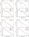 |
Fig. 3 Dependence of optical properties on grain shape (left) and size (right) for silicate grains made of aSil-1/a-C2.5nm materials (top) and carbonaceous grains with a-CH/a-C10nm composition (bottom). Each block of figures presents the total absorption and scattering efficiencies as solid and dashed lines (upper figure), respectively, and the polarisation efficiency Qpol = (β2,ext − β1,ext)/2 (lower figure). For comparison, Qpol for THEMIS I oblate silicates with e = 1.3 and variable size are shown in the lower figure of the top right block. |
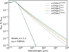 |
Fig. 4 Dependence of optical properties on grain composition for carbonaceous grains with a-CH/a-C2.5nm, a-CH/a-C4nm, a-CH/a-C5nm, a-CH/a-C6nm, and a-CH/a-C10nm compositions in grey, brown, orange, green, and blue, respetively (aeff = 100 nm, oblate with e = 1.3). Solid lines show Qabs and dashed lines Qsca. |
4.2 Grain densities
Figure 6 shows the volume densities of spheroidal core-mantle grains with either carbon or silicate cores for 1.3 ⩽ e ⩽ 2. The shape and elongation have little influence on density with less than 1.5% and 0.7% variations in the case of silicate and carbonaceous grains, respectively. However, the large variation in the core-to-mantle volume ratio as a function of size leads to a variation in the volume density of about +30% for silicates and −20% for carbonaceous grains when aeff increases from 25 to 700 nm. The dust SED being inversely proportional to the grain density, the aforementioned variations will be accounted for when producing both total and polarised SEDs.
5 Observational constraints
A wide range of observational constraints are used to define the state of the THEMIS 2.0 chemical composition, size distribution and dust-to-gas mass ratio. In addition to the constraints already presented in Sect. 2.1.1, the defining model parameters are tested against the spectral energy distribution from the mid-IR to the millimetre range and the extinction from the UV to the mid-IR, total and polarised quantities in both cases. One of the most important points is to have as much coherent data as possible that is representative of the same type of weakly irradiated diffuse medium with low column density. To define the dust-to-gas mass ratios of each dust population, one must know how the extinction scales with the gas column density (assuming a perfect mixing of gas and dust along the line of sight). This is usually described by the quantity NH/E(B − V) which was recently shown to vary with increasing value from the Galactic plane to regions at higher latitude (i.e. from high to low column density regions, see for instance references in Ysard 2020; Hensley & Draine 2021; Siebenmorgen 2023). The range of measured values is fairly wide, ranging from around 4 to 9 × 1021 cm−2 mag−1 (see for instance Bohlin et al. 1978; Liszt 2014; Planck Collaboration XI 2014; Lenz et al. 2017; Murray et al. 2018; Nguyen et al. 2018; Remy et al. 2018; Van De Putte et al. 2023). In agreement with and to be comparable with the models of Hensley & Draine (2023) and Siebenmorgen (2023), we adopt the value measured by Lenz et al. (2017), NH/E(B − V) = 8.8 × 1021 cm−2 mag−1, as representative of low column density high latitude lines of sight. However, to test the impact of the uncertainty of this parameter, we also consider the Bohlin’s ratio, NH/E(B − V) = 5.8 × 1021 cm−2 mag−1 (see details in Sect. 5.5).
Hensley & Draine (2021) recently presented a review of the observational constraints available in the literature, the aim being to bring them together in a coherent way to make a reference dataset on which to test dust models for the diffuse ISM. In the following, we use part of this dataset but sometimes depart from it for reasons that are detailed in the next sections.
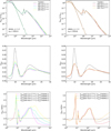 |
Fig. 5 Dependence of optical properties on grain composition for silicate grains with cores made of aSil-1, aSil-2, aSil-3, and aSil-4 materials in pink, blue, green, and yellow, respectively (aeff = 100 nm, oblate with e = 1.3) on the left and cores made of aSil-5, aSil-6, and aSil-7 in red, brown, and orange, respectively, on the right. Top: solid lines show Qabs and dashed lines Qsca. Middle: zoom in on the silicate mid-IR features. Bottom: ratios of Qabs to THEMIS I. |
5.1 Element abundances in the solid phase
Hensley & Draine (2021) proposed numerical values derived from the literature. It should be noted, however, that estimating the abundance of elements is a complicated exercise and that variations of greater or lesser magnitude depending on the elements and the lines of sight have been observed (e.g. Jenkins 2009). De Cia et al. (2021) recently highlighted spatial variations in the metallicity in our Galaxy by a factor greater than 10. Moreover, as pointed out by Compiègne et al. (2011), the existence of a stellar standard representative of the diffuse ISM is questionable. Should we start from the solar abundance, the enhanced solar abundance following a Galactic Chemical Enrichment model (GCE, Bedell et al. 2018), or from F, G-type stars? This choice already leads to a difference in the total abundance of up to 90 ppm for carbon or to more than 200 ppm for oxygen (cf. Compiègne et al. 2011; Hensley & Draine 2021). As shown by Mishra & Li (2017), the various methods used to determine [Si or C/H]dust also lead to different estimates (dust model-dependent or -independent methods).
Carbon is an element that appears to cycle rapidly between the gas phase and the solid phase (Jones et al. 2014), which is highlighted by depletion measurements. Sofia et al. (2011) made the first estimates of the abundance of carbon in the gas phase using the strong transition at 1334 Å rather than the weak feature at 2325 Å. This resulted in more reliable estimates of the abundance of carbon in the gas that are systematically lower than estimates based on the 2325 Å feature. On average, they found an additional 80 ppm available for the solid phase. Using this method, Parvathi et al. (2012) measured in the diffuse medium 100 < [C/H]dust ≲ 290 ppm.
The amount of silicon included in the silicate grains is also uncertain. The measurements range from [Si/H]dust ~ 15 to 40 ppm depending on the studies (e.g. Sofia & Meyer 2001; Compiègne et al. 2011; Nieva & Przybilla 2012; Hensley & Draine 2021). Voshchinnikov & Henning (2010) have also shown a variation in the amount of silicon locked in grains correlated with the Galactic latitude.
Insofar as elemental abundances appear to vary from one line of sight to another, we impose no other limits on the models than to respect the following three criteria based on the articles cited above: 100 < [C/H]dust ≲ 290 ppm, 15 ≲ [Si/H]dust ≲ 40 ppm and [Mg/H]dust ≲ 60 ppm. This allows all the other abundances to be in line with the different values presented in the articles cited above and the references therein.
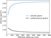 |
Fig. 6 Core-mantle spheroidal grain volume densities. The blue line shows the case of grains with silicate cores with 5 nm-thick a-C mantles and the black line of a-C:H cores with 20 nm-thick a-C mantles. The thickness of the lines shows the little dispersion of the density as a function of the grain shape, oblate or prolate, and elongation. |
5.2 Total SED
From far-IR to sub-millimetre, Hensley & Draine (2021) tabulated colour-corrected estimates with uncertainties based on Planck Collaboration results (Planck Collaboration Int. XVII 2014; Planck Collaboration Int. XXII 2015; Planck Collaboration XI 2020). This SED is an average SED for lines of sight with NHI ~ 3 × 10²⁰ H cm−2 and we adopt it in the following (see their Table 3). We further include the measurements made by Bianchi et al. (2017) at 250, 350, and 500 µm, by correlating the Herschel Virgo Cluster survey data (HeViCs) with HI observations from the Arecibo Legacy Fast ALFA (ALFALFA). As shown by Hensley & Draine (2021), the two datasets agree perfectly.
In the mid-IR, Hensley & Draine (2021) use a Spitzer IRS spectrum observed by Ingalls et al. (2011) in the direction of the translucent cloud DCld 300.2-16.9. This cloud, which has a column density of the order of 4 × 10²¹ H cm−2, that is, 10 times higher than the regions used for the far-IR to sub-millimetre part of the spectrum, was affected by supernovae explosions 2 to 6 × 10⁵ years ago. Shortwards of 5 µm, an average spectrum of star-forming galaxies is added from Lai et al. (2020). Hensley & Draine (2021) then normalise these two spectra to the DIRBE photometric measurements of Dwek et al. (1997). Since the size distribution of sub-nanometre sized carbon grains, whether PAHs or amorphous hydrocarbons, is strongly affected by shocks and intense radiation fields, the two aforementioned spectra may not be representative of the weakly irradiated diffuse ISM used for the far-IR to sub-millimetre part of the SED. We thus choose not to include any spectrospic data as none exists to date for the diffuse medium at high latitude8. In conclusion, for the mid-IR part, we follow Compiègne et al. (2011) who selected regions of the sky at latitudes |b| > 15° and NH < 5.5 × 10²⁰ H cm−2, avoiding point sources, nearby molecular clouds and the Magellanic clouds. This leads to the inclusion of only four mid-IR data points in the DIRBE filters at 3.53, 4.9, 12, and 25 µm.
5.3 Polarised SED
We adopt the polarised far-IR to sub-millimetre SED described by Hensley & Draine (2021) which is based on the results of Planck Collaboration Int. XXII (2015) and Planck Collaboration XI (2020). The dust model must be able to reproduce all cases and we therefore adopt the maximum polarisation of 19.6% at 353 GHz derived by Hensley & Draine (2021) which leads to a polarised emission per hydrogen of 2.51 × 10⁻²⁸ erg s−1 sr−1 H−1 at 353 GHz.
Comparing the results of the Planck Collaboration with those of BLASTPol (at 250, 350, and 500 µm, Ashton et al. 2018), Hensley & Draine (2021) conclude that the polarisation fraction from 250 µm to 3 mm is essentially constant. To reach this conclusion, Hensley & Draine (2021) use the Planck SED for the diffuse medium and λ ⩾ 850 µm. The BLASTPol data come from observations in the direction of the translucent molecular cloud Vela C detected in CO, which lies in the Galactic plane and for which the column density is estimated to be around 5 × 10²¹ H cm−2, that is, more than one order of magnitude higher than those lines of sight used to produce the Planck SEDs. Studies of comparable translucent clouds have shown that dust is already expected to have significantly grown by coagulation at such column densities (e.g. Ysard et al. 2013; Fanciullo et al. 2017). All grains are then mixed and can easily explain why such a ratio would be flat at all wavelengths.
The nature of the regions observed is therefore sufficiently different to warrant at least a cautious warning when comparing the polarisation fraction wavelength-dependency with models designed for the high-latitude diffuse ISM. We therefore do not include this ratio in our fits, as we do not consider it to be binding. We only present the comparison with the results obtained to allow comparison with other dust models (Hensley & Draine 2023; Siebenmorgen 2023).
5.4 Total extinction
The extinction in the UV has been extensively investigated and Hensley & Draine (2021) present a review of the various studies made since the 1980s. Most of the measurements are consistent and the dispersion over the lines of sight is relatively limited. In the following, we include the observations presented by Cardelli et al. (1989), Gordon et al. (2009) and Fitzpatrick et al. (2019) for λ ⩽ 0.4 µm. In the visible (0.4 ⩽ λ ⩽ 1 µm), we also follow the prescription of Hensley & Draine (2021), based on the results of Schlafly et al. (2016) and Wang & Chen (2019). Most dust models try to reproduce the standard value RV = A(V)/E(B − V) = 3.1 which corresponds to the average value measured in the Milky Way (see for instance Fitzpatrick et al. 2019, and references therein). It is important to note, however, that RV, like most of the parameters used to define grains in the diffuse ISM, can vary significantly from one line of sight to another. As described by Siebenmorgen et al. (2023), the OB stars often used to measure the reddening curve are generally at a great distance and the lines of sight therefore pass through several individual interstellar clouds, simulating a more or less constant - average -value of RV. Selecting 53 well characterised single-cloud lines of sight (distances, spectral types) they find variations between 2 ≲ RV ≲ 4.3 and an average of 3.1 ± 0.4. This is similar to the results of Decleir et al. (2022) who find values between 2.4 ≲ RV ≲ 5.3 for lines of sight with 0.8 ≲ A(V) ≲ 3, while respecting the 3.1 average value.
The extinction curve in the near-IR (1 ≲ λ ≲ 4 µm) is usually represented by a power law A(λ) ∝ λ−α. Recent photometric measurements agree on a value of α around 1.7–1.8 in the diffuse ISM (e.g. Chen et al. 2018; Nagatomo et al. 2019; Wang & Chen 2019), which was confirmed by the first spectroscopic extinction curve measurements made by Decleir et al. (2022) between 0.8 and 5 µm. For a range of measured values between 1.4 to 2.2, they found an average for the diffuse ISM of α = 1.71 ± 0.01. These results are in agreement with older determinations such as those of Rieke & Lebofsky (1985), Cardelli et al. (1989) and the lines of sight with the lowest extinction in McClure (2009). Hensley & Draine (2021) deviate from this and choose to set α = 1.55, which gives a much flatter extinction. We do not follow them and therefore use the recent extinction curves referred to above. Their choice appears to be motivated by the shape of the mid-IR extinction that they adopt.
In the mid-IR (4 ≲ λ ≲ 35 µm), Hensley & Draine (2021) built on the work of Hensley & Draine (2020) for the determination of the silicate band profiles at ~ 10 and 18 µm. Their observations were made in the direction of Cyg OB2-12 which has an A(V) of ~ 10. This line of sight shows a definite flattening for 4 ≲ λ ≲ 8 µm. This result is in agreement with other studies towards regions with similar relatively high A(V) either in the direction of the Galactic plane or of dark clouds such as the Coalsack nebula (e.g. Indebetouw et al. 2005; Gao et al. 2009; Wang et al. 2013, 2015; Xue et al. 2016) and which can be modelled with grain models including significant grain growth compared to dust in the diffuse ISM (Weingartner & Draine 2001). These lines of sight are a priori significantly different from the high latitude lines of sight used to determine total and polarised SEDs with column densities below a few 1020 H cm–2. However, more recent measurements have since been reported by Gordon et al. (2021), based on Spitzer IRS, IRAC, and MIPS data: some of their sightlines have quite high A(V) as in previous studies but nine of them have A(V) < 3. When looking at their Fig. 5 in which the extinction curves are ranked according to the dust column density, we see two things: (i) no strong flattening shortwards of 8 µm; (ii) the band-to-continuum ratio decreases with decreasing column density. The spectral shape shortwards the 10 µm silicate feature appears to be consistent with previous studies and the 10 µm silicate feature itself is compatible with those presented in Chapman et al. (2009, sightlines with the lowest extinction) and van Breemen et al. (2011). Since the extinction curves measured by Gordon et al. (2021) with A(V) < 3 are more representative of the high latitude low density regions used to characterise the total and polarised SEDs, we use them in the following. To combine these mid-IR extinction data with those in the near-IR by Decleir et al. (2022), it would be best to perform a joint analysis using the same reference stars for both datasets in order to get a more reliable slope from near- to mid-IR. Similarly, the extrapolation to infinite wavelengths that is used to estimate A(V) would benefit from being re-done fitting all near- to mid-IR data simultaneously9. However this is beyond the scope of this paper and in the following, we simply normalise the mid-IR results of Gordon et al. (2021) to the near-IR results of Decleir et al. (2022) at λ = 5 µm.
5.5 Polarised extinction
In accordance with the literature presented by Hensley & Draine (2021), the UV to near-IR extinction is represented by a Serkowski law (Serkowski et al. 1975):
![Mathematical equation: $p/{p_{\max }} = \exp \left[ { - K{{\ln }^2}\left( {{\lambda _{\max }}/\lambda } \right)} \right]$](/articles/aa/full_html/2024/04/aa48391-23/aa48391-23-eq10.png) (6)
(6)
with K = 0.87 and λmax = 0.55 µm from 0.12 to 1.38 µm; a power law with β = 1.6 is adopted for 1.38 ⩽ λ ⩽ 4 µm. It is worth noting, however, that measurements of λmax along dif fuse to translucent lines of sight, out of the Galactic Plane have shown that it increases with the visual extinction A(V) For instance, Vaillancourt et al. (2020) show variations from λmax = 0.43 to 0.72 µm for A(V) ⩽ 4, which can be approximated by the linear relationship λmax ~ 0.51 + 0.02A(V).
As for the polarised emission, the model should be able to reproduce the maximum polarisation, which is usually expressed in the V band per unit reddening pV/E(B − V), assuming that RV = 3.1. Compared to the classical value of 9% per mag (e.g. Serkowski et al. 1975), this maximum has recently been revised upwards in two studies. For the low column density lines of sight used to estimate the total and polarised SEDs, Planck Collaboration XII (2020) found a maximum value of about pV/E(B − V) ~ 13%. Panopoulou et al. (2019) found that 13% is only a lower limit. They could linearly fit their data with a value of 15.9 ± 0.4% and found that all their lines of sight had pV/E(B − V) < 20%. Similar results were also found by Angarita et al. (2023).
Given the uncertainty in the measurement of the polarised extinction, we make different fits in the following, one with a normalisation at pV/E(B − V) = 13% and one using the low classical value of 9%. As stated in Sect. 5, we choose to first normalise our model to Lenz et al. (2017). If instead we nor-malise to the lower value previoulsy measured by Bohlin et al (1978), a maximum optical polarisation of 13% (9%) would be equivalent to a maximum of 19.7% (13.6%) in the normal-isation frame of Lenz et al. (2017). Bohlin et al. (1978) and Lenz et al. (2017) thus roughly encompass the dispersion in NH/E(B − V) measured until now10 (e.g. Liszt 2014; Planck Collaboration XI 2014; Nguyen et al. 2018; Remy et al. 2018; Zuo et al. 2021; Van De Putte et al. 2023).
A handful of polarisation measurements in the 3.4 µm hydrocarbon band were also made towards the Galactic Centre (Adamson et al. 1999; Chiar & Tielens 2006), three young stellar objects (Ishii et al. 2002) and a Seyfert 2 galaxy (Mason et al. 2007). All the studies either only measured upper limits or very low values, compatible with a non-polarised band. For instance, Chiar & Tielens (2006) observed two Galactic Centre sources, GCS-3II and GCS-3IV, for which they measured Δp3,4µm = 0.06 ± 0.13% and 0.15 ± 0.31%, respectively. We do not include these values in our fitting procedure but compare them a posteriori with our results to allow comparison with other models (e.g. Siebenmorgen 2023; Hensley & Draine 2023). The observed lines of sight are indeed too different from those used to produce the total and polarised SEDs to be used as binding constraints. A measurement of the polarisation in the 10 µm-silicate band has also been made by Telesco et al. (2022) in the direction of Cyg OB2-12: they find p10.2 µm = (1.24 ± 0.28)%. Combining this measure with that of McMillan & Tapia (1977), Hensley & Draine (2021) find p10.2 µm/p0.55 µm = 0.014 ± 0.03. This gives an interesting float point for dust models but again, due to the disparity with the lines of sight used to build the total and polarised SEDs, we do not use it as a binding constraint in our fitting routine but only compare it with our results afterwards.
5.6 Sub-millimetre to visible observational ratios
Planck Collaboration XII (2020) also estimated two interesting ratios to test dust models: RP/p = P353GHz/pV, the ratio of the polarised intensity in the sub-millimetre to the degree of polarisation in the visible, and RS/V = (P/I)353GHz/(p/τ)V, the ratio of the submillimetric to visible polarisation fractions. They found RP/p = 5.4 ± 0.5 MJy sr1 mag1 and RS/V = 4.2 ± 0.5. In con-strast to the all-sky study performed by Planck Collaboration XII (2020), Panopoulou et al. (2019) restricted themselves to a sky area with a high submillimetric polarisation fraction of ~20%, similar to that of the polarised SED defined in Sect. 5.3, and found RP/p = 4.1 ± 0.1 MJy sr1 mag1. In the following, these ratio values are not included in our fitting routine, but we compare our results against them retrospectively.
5.7 Interstellar radiation field
With fixed grain properties, the SED then only depends on the radiation field. The choice of the radiation spectral shape and intensity therefore affects the final estimation of the gas-to-dust mass ratio. We fix its spectral shape to that of Mathis et al. (1983) at a galactocentric distance of 10 kpc, scaled by the G0 factor11. Fanciullo et al. (2015) showed that the ISRF intensity varies in the diffuse ISM as at most 0.5 ≲ G0 ≲ 1.8.
6 THEMIS 2.0 definition
From the laboratory and astronomical data presented above, the model can now be defined. We first present the methodology of our adjustments, the associated results, and finally define the new version of THEMIS.
6.1 Grain alignment
The polarisation of radiation comes from the alignment of aspherical grains with the magnetic field, this alignment being made possible by the magnetic properties of the grains. The detailed explanation of grain alignment, which is beyond the scope of this paper, has made great progress in the last decade both theoretically and observationally (e.g. Andersson et al. 2015; Hoang & Lazarian 2016; Lazarian 2020; Hoang et al. 2023).
It is widely accepted that interstellar silicates contain iron, so these grains are paramagnetic and can align themselves effectively with the magnetic field. In most models of interstellar grains, the population of large carbons is usually represented by graphite, a diamagnetic material, which cannot align effectively with the magnetic field. Indeed, graphite paramagnetic properties only arise from the rotation of charged grains or hydrogen attachment to the surface, both resulting in weak magnetic moments (see for instance Hoang & Lazarian 2016). However, THEMIS does not assume graphite but instead hydrogenated amorphous carbons. A paramagnetic defect in a disordered hydrocarbon lattice can be defined by an electronic configuration with an unpaired spin that gives rise to an electronic state close to the Fermi level (Delpoux 2009). For a lattice composed entirely of sp3 carbons, defects are sp3 sites with dangling bonds. In the case of a material containing both sp2 and sp3 carbons, two types of defects can be observed. The first is an isolated dangling bond. The second, any cluster with an odd number of sp2 sites generates a Fermi state. The magnetic moment of an a-C:H grain therefore depends on the concentration of paramagnetic defects in the material (e.g. Esquinazi & Höhne 2005; Akhukov et al. 2013; Sakai et al. 2018). This concentration has been estimated experimentally for amorphous hydrocarbons in meteorites (Binet et al. 2002, 2004) for which it is comparable to the paramagnetic defects in silicates (Delpoux 2009).
The theoretical study carried out by Hoang et al. (2023) shows that if a-C:H grains larger than 50 nm are present in the diffuse ISM, they can produce significant polarisation due to efficient internal alignment and B-RAT alignment (see their Sect. 7). They further suggest to test this finding against measurement of the polarisation in the 3.4 µm hydrocarbon feature.
While we do not consider the possibility of iron inclusions in a-C(:H) materials, we point out that their doping with sulphur atoms can induce magnetic properties, as highlighted by Jones (2013). Thus, there appears to be no reason why a-C(:H) grains should not be aligned. In what follows, we therefore assume that the two populations of large grains can align with the magnetic field but remind the reader that the concentrations of free radicals and impurities with uncompensated electron spins as well as the possibility of iron inclusions are still uncertain for the diffuse ISM carbonaceous dust (see for instance Lazarian 2020).
6.2 Methodology
We have seven types of silicates and five types of large core-mantle carbonaceous grains, each for two oblate and two prolate shapes. As we have no prior knowledge, we test the association of all carbonaceous and silicate grains, the populations being allowed to have identical or different shapes. In the same way, we test the cases of a universal grain alignment law or a differentiated alignment between amorphous hydrocarbons and silicates. We consider three free parameters for the analytical alignment function defined by Eq. (5): ƒmax, athresh and pstiff. The radiation field is allowed to vary within the limits defined in Sect. 5.7.
To perform the fits, we use the DustEMWrap12 DDL extension of the DustEM code. DustEMWrap allows for iterative fitting of SEDs and extinction curves, including the fit of linear polarisation (Stokes parameters I, Q, and U). The total and polarised SEDs are fitted together with the Serkowski law. The model total extinction is only a posteriori qualitatively compared to the observations which are too widely spread to be included in the fitting routine. Our focus points at that stage are mainly the slope in the near-IR and the shape and intensity of the two mid-IR silicate features. The polarisation fraction is not included in the fit either, but simply compared a posteriori with the results for the reasons given in Sect. 5.3. Finally, elemental abundances are calculated after the fitting procedure and we exclude models that do not comply with the limits given in Sect 5.1.
6.3 Fitting results
The fitting results and the associated parameters for defining the dust model are shown in Figs. 7–10. As expected from Fig. 5, the mid-IR silicate features are not very strong but agree with half of the lines of sight with A(V) < 3 presented by Gordon et al. (2021). This illustrates just how crucial an out-of-Galactic plane diffuse extinction curve (A(V) < 1) would be for calibrating grain models13. As a complement, Appendix A shows the contributions of the different grain populations to total and polarised emission and extinction (Figs. A.1–A.3). For comparison, fitting results obtained with THEMIS I silicates are presented in Figs. C.1–C.4.
We can see that the new silicates derived from laboratory measurements make it possible to explain the UV to cm observations without violating the constraints on the abundance of the various elements making up the grains. Two comments can be made about grain composition, independent on the data normalisation: (i) all the silicate mixtures can explain the observations; (ii) all the mantle descriptions for a-C:H/a-C lead to acceptable fits, with the exception of a-C2.5nm (same result if THEMIS I silicates are used instead of lab-derived silicates). The first comment agrees with the constraints derived from the X-ray and mid-IR observations presented in Sect. 2.1.1 showing that silicates are a mixture of olivine and pyroxene stoichiometry mineralogies. This makes it difficult to conclude on the proportion of one type of silicate to the other from this study. This is not particularly surprising, since this proportion is bound to vary according to local physical and chemical conditions (Demyk et al. 2001; Psaradaki et al. 2023). The second comment gives indications on the evolution of carbons formed around evolved stars in the a-C:H form and then evolving to become a-C:H/a-C. The exclusion of the a-C2.5nm shows that the formation of aromatic mantles cannot originate entirely from nano-grain accretion but must be, at least partly, due to the photo-processing of the grain surfaces in agreement with what was presented in Jones et al. (2013, and references therein).
Whether we force the two populations of carbonaceous and silicate grains to have the same shape, or allow the two populations to have different shapes, then the four shapes tested here lead to reasonable fits matching the observations at ~±20% at almost all wavelengths (see Fig. B.1). Not being restrictive on this point seems reasonable, since we can see no physical reason why all the grains in the ISM should have exactly the same shape. Similarly, the alignment function depends on the optical properties and shape of the grains under consideration to obtain the same polarisation levels. We thus find solutions with a universal alignment function for both populations as well as different alignment functions, whether or not the grains are the same shape, owing to the flexibility of our parametric alignment function (see Eq. (5) and Figs. 5, A.4). This is again independent on the choice made for the data normalisation. Furthermore, the vast majority of acceptable models do not require perfect grain alignment, but rather 0.6 ≲ ƒmax ≲ 0.9. This means that whatever the NH/E(B − V) normalisation chosen, our models are able to reproduce the high levels of polarisation found by Panopoulou et al. (2019) and Angarita et al. (2023) since there is still room to increase ƒmax for almost all combinations of compositions and shapes.
Although this constraint was not used in our fitting routine (see Sect. 5.3), as already shown by Siebenmorgen (2023), two polarising grain populations can explain the relative constancy of the polarisation fraction from the far-IR to sub-millimetre (Fig. 7). Depending on the mass ratio between the silicates and the carbonaceous grains, as well as on their alignment functions, the models can generate a flat, slightly increasing or slightly decreasing tendency. THEMIS I silicates are also able to reproduce this trend (Fig. C.4). To be able to really understand the differences, or lack of them, in the spectral variations of total and polarised emissions, detailed studies of diffuse regions will have to be carried out rather than working on average SEDs as here.
Finally, Fig. 8 zooms in on the spectral profile of the hydrocarbon band at 3.4 µm. In all cases and whatever the chosen normalisation, the polarisation excess above the continuum is below the upper limits measured by Chiar & Tielens (2006, see Sect. 5.5) with Δp3,4µm ⩽ 0.07 and 0.08% (0.09 and 0.13%) for a normalisation at pV/E(B − V) = 9 and 13%.mag−1, respectively, with the Lenz’s ratio (with the Bohlin’s ratio). In the case of a normalisation to the Lenz’s ratio, about 20 to 30% of the acceptable models shown in Fig. 7 are even compatible with no polarisation at 3.4 µm. This proportion falls to between ~5 to 16% for a normalisation to the Bohlin’s ratio.
6.4 Variations in the diffuse ISM
The Planck data revealed a variability in the properties of dust in the diffuse medium (1019 ⩽ NH ⩽ 2.5 × 10²⁰ H cm−2, Planck Collaboration XI 2014). Their results were based on a pixel-by-pixel modified blackbody χ2-fit between 353 and 3 000 GHz:
 (7)
(7)
where  is the optical depth at ν0 = 353 GHz, T is the dust colour temperature, and β is the spectral index assumed to be constant from 100 µm to 353 GHz. Besides, Planck Collaboration XI (2014) computed the dust luminosity LH = (∫vIvdv)/NH and opacity
  . Using the Sloan Digital Sky Survey data (SDSS, Schneider et al. 2010), they also derived the dust optical extinction E(B − V). Their results showed that (i) the dust luminosity does not vary with temperature, that (ii) the opacity and (iii) the spectral index are anti-correlated with the temperature, and (iv) presented E(B − V) vs. τ353GHz for high-latitude diffuse lines of sight with 1019 ⩽ NH ⩽ 2.5 × 10²⁰ H cm−2. None of these results can be explained for constant grain properties. In Ysard et al. (2015), we explored how variations in the grain structures or abundances and in the radiation field intensity could explain these variations. Here we explore how the dispersion of models can explain the observations along the lines of sight with the highest polarisation fractions (Fig. 7) compared to the variations described in Planck Collaboration XI (2014).
To be able to compare our models with the dust parameters derived in Planck Collaboration XI (2014), we perform similar modified blackbody χ2-fit for all the models presented in Fig. 7. Figure 11 shows that our collection of models can account for most of the parameters observed and that this depends neither on the NH/E(B − V) normalisation choice nor on the maximum level of polarised extinction. If only the (in)homogeneity of the carbon mantles were taken into account, then the dispersion of the measurements could not be reproduced. The diversity of the chemical composition of silicates must be taken into account (see Fig. C.5 for instance, where only THEMIS I silicates are considered). Performing the fitting procedure with various polarisation fractions or with slightly different SEDs, would also help to fully populate the plots in Fig. 11.
Figure 12 presents the comparison of our best fits with the RP/p and RS/V ratios, along with the distributions of the λmax, p10.2 µm/p0.55 µm, and RV parameters. Our models calibrated on the Lenz’s ratio and pV/E(B − V) = 9% are compatible with the values of RP/p measured by Planck Collaboration XII (2020) whereas those calibrated at 13% are rather compatible with the values measured by Panopoulou et al. (2019). Those calibrated on the Bohlin’s ratio and pV/E(B − V) = 9% are between the two, while those taking Bohlin’s and 13% are weaker overall. This illustrates once again that the variability of the silicate chemical compositions can explain the observed variations. Similarly, all our models are consistent with the measurements of RS/V. For comparison, Fig. 12 also shows the ratios given by the model of Hensley & Draine (2023) which are within the uncertainties given by Planck Collaboration XII (2020), both on the weak ratio side. Whatever their normalisation, most of our models have λmax values ranging between 0.50 and 0.51 µm. This is smaller than the usual 0.55 µm used to build the Serkowski curve but fully consistent with the measures made by Vaillancourt et al. (2020) towards low extinction lines of sight. For comparison, Hensley & Draine (2023) give a higher value of λmax = 0.59 µm, also compatible with the observations. The polarised extinction 10 µm-silicate feature normalised to the optical of our models range from 0.03 ⩽ p10.2 µm/p0.55 µm ⩽ 0.07, with most of them lying around 0.05. This is a factor of about 2 to 4.7 smaller than the value inferred from the observations towards Cyg OB2- 12 of Telesco et al. (2022) and McMillan & Tapia (1977). In contrast to our predictions, Hensley & Draine (2023) predict p10.2 µm/p0.55 µm = 0.23, about 1.6 higher than the observations. This is probably linked to the fact that their model overpredicts the total extinction at this same wavelength (see their Fig. 5) whereas our predictions are quite lower in this same wavelength range. It is however difficult to conclude anything from that considering how much the mid-IR total extinction curve is different when moving from the Galactic Plane or Centre to higher latitudes (see for instance Gordon et al. 2021). Observations of this polarised extinction feature at higher latitude would be beneficial for constraining dust models. Finally, apart from the models normalised to the Bohlin’s ratio with pV/E(B − V) = 9%, most of our models have RV values that are larger than the average 3.1 but all remain consistent with the dispersion measured by Decleir et al. (2022) for lines of sight with 0.8 ≲ A(V) ≲ 3.
 |
Fig. 7 Data are those presented in Sect. 5. From top to bottom and left to right, the figures first show the models against the observations: total SED, polarised SED, polarised extinction, total extinction; and then some model parameters: radiation field, silicon abundance, magnesium abundance, oxygen abundance, iron abundance, sulphur abundance, and carbon abundance. The light coloured areas represent the dispersion of the models in agreement with the observations and the matching thick solid lines show the best fits (see Sect. 6.3 for details). As detailed in the text, two gas-to-dust mass ratios and two maximum optical polarisation values are considered to normalise the models. The models normalised to the ratio of Lenz et al. (2017) are shown in magenta and orange for pV/E(B − V) = 9% and 13%, respectively. Those normalised to the ratio of Bohlin et al. (1978) are shown in green and blue for pV/E(B − V) = 9% and 13%, respectively. |
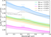 |
Fig. 8 Same colour scheme as in Fig. 7. Zoom on the 3.4 µm hydrocarbon feature seen in polarised extinction. The dashed lines show the upper limits measured by Chiar & Tielens (2006) towards GCS 3-II and GCS 3-IV, lowest and highest lines, respectively, above the continuum of our four best-fit models (see Sect. 6.3 for details). For comparison, we also show in grey the model of Hensley & Draine (2023) which complies with the upper limit measured towards GCS 3-IV but not with the lower one towards GCS 3-II. Hensley & Draine (2023) gives indeed ∆p3.4 µm 2 to 2.6 times as large as our best models. |
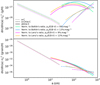 |
Fig. 9 Same colour scheme as in Fig. 7. Top: grain mass distributions of the best-fit models shown in Fig. 7. Bottom: equivalent grain number distributions. In both figures, the distributions for the amorphous nano-carbon grains, a-C, are shown as dotted lines, for the a-C:H/a-C grains as dashed lines and for the aSil/a-C grains as solid lines. |
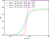 |
Fig. 10 Alignment functions of the best fits presented in Fig. 7 and Sect. 6.3. The colour scheme is the same as in Fig. 7. Models normalised to the ratio of Lenz et al. (2017) are shown by magenta and orange lines for pV/E(B − V) = 9% and 13%, respectively. Both models are for pro-lates with e = 2. Those normalised to the ratio of Bohlin et al. (1978) are shown by green and blue lines for pV/E(B − V) = 9% and 13%, respectively. The model plotted in green is for oblates with e = 1.3 and the one in blue for prolates with e = 2. |
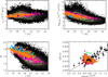 |
Fig. 11 Variations in the dust parameters presented by Planck Collaboration XI (2014), based on a pixel-by-pixel modified blackbody χ2 fit (see Eq. (7) and Sect. 6.4 for details). In the top left and right, and the bottom left figures, the observational results are the density of points maps, on which we overplot yellow contours: the central contour encloses 50% of the observed pixels and the external contour 75%. In the bottom right figure, the observational results are the black dots with error bars. In the four figures, the model results are the coloured dots, with the same colour scheme as in Fig. 7. Models normalised to the ratio of Lenz et al. (2017) are shown by magenta and orange dots for pV/E(B − V) = 9% and 13%, respectively. Those normalised to the ratio of Bohlin et al. (1978) are shown by green and blue dots for pV/E(B − V) = 9% and 13%, respectively. For comparison, the dark blue squares show the parameters derived from the model of Hensley & Draine (2023). Top left: luminosity vs. temperature. Top right: opacity at 353 GHz vs. temperature. Bottom left: spectral index vs. temperature. Bottom right: E(B-V) vs. optical depth at 353 GHz, models shown for NH = 1020 H cm−2. |
6.5 Final model
The THEMIS model is public14. It is fully integrated into the DustEM numerical code15, which is used to produce all the figures in Figs. 7, 9, and 10. All the optical properties calculated for the chemical compositions and mantle description presented in Sect. 2 can be accessed at these two addresses and used in the DustEM and DustEMWrap codes.
We also provide the best fits (thick lines in Figs. 7, 9, and 10) for the four normalisations considered here and which are obtained for:
aSil-4/a-C2.5nm (oblates, e = 1.3) and a-CH/a-C4nm (prolates, e = 2) in the case of a normalisation to the Bohlin’s ratio and for pV/E(B − V) = 9%;
aSil-1/a-C2.5nm (prolates, e = 2) and a-CH/a-C5nm (prolates, e = 2) in the case of a normalisation to the Bohlin’s ratio and for pV/E(B − V) = 13%;
aSil-4/a-C2.5nm (prolates, e = 2) and a-CH/a-C6nm (prolates, e = 1.3) in the case of a normalisation to the Lenz’s ratio and for pV/E(B − V) = 9%;
aSil-2/a-C2.5nm (prolates, e = 2) and a-CH/a-C5nm (prolates, e = 2) in the case of a normalisation to the Lenz’s ratio and for pV/E(B − V) = 13%.
From now on, this last model will be considered as the THEMIS 2.0 reference model (see Table 3 for the main model parameters). However, it should be borne in mind that all the models shown in Figs. 7, 9, and 10 are compatible with all the observations available within ±20%. When making a comparison with a particular dataset, it may therefore be useful to try to see which normalisation is the most relevant, and not to confine oneself to using a single combination of compositions, size distribution or alignment function. The authors of this study will be happy to discuss the relevance of the choice of properties should the need arise.
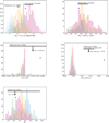 |
Fig. 12 Histograms of parameters derived from our best fits represented with the same colour scheme as in Fig. 7. For comparison, the parameters derived from the model of Hensley & Draine (2023) are shown by the dark blue squares. The two figures in the top row show two characteristic ratios of the polarised observations made with the Planck satellite: RP/p and RS/V. The measurements, including their uncertainties, made by Panopoulou et al. (2019) and Planck Collaboration XII (2020), are represented by the black horizontal lines. The two figures in the middle row show the dispersion of λmax (left) and of the polarised extinction at 10 µm normalised to the optical (right) of our best fits. The measurements, including their uncertainties, made by Vaillancourt et al. (2020) and Telesco et al. (2022) combined to McMillan & Tapia (1977) are shown by the black horizontal lines. The bottom row figure shows the histogram of the extinction parameter RV. The measurements made by Decleir et al. (2022), including their uncertainties, are shown by the black horizontal line. |
Main parameters defining the best dust model normalised to the Lenz’s ratio and pV/E(B − V) = 13%mag-1 as in Siebenmorgen (2023) and Hensley & Draine (2023).
7 Conclusion
THEMIS is a dust model that includes three compact dust populations: a population of (sub-)nanometric aromatic-rich amorphous carbon a-C grains, a population of larger core-mantle a-CH/a-C carbonaceous grains, and a population of core-mantle a-Sil/aC silicates. We have extended the THEMIS grain model, first described in Jones et al. (2013), in three different ways. First, the most comprehensive laboratory data on silicates to date were used to calculate the optical properties of this grain population. Second, the homogeneity of the a-C mantles at the surface of the a-C:H/a-C grains was studied. Third, spheroidal grains were considered instead of spheres in order to account for polarised emission and extinction.
This new version of THEMIS, for the first time entirely based on laboratory measurements, reproduces the dust emission and extinction, both total and polarised, observed in the diffuse ISM at a high Galactic latitude, while respecting the constraints on the abundances of the various elements making up the grains. An interesting point is that the model has not been pushed to its limits yet since it does not require the perfect alignment of all grains to explain the observations (ƒmax < 1 in Eq. (5) and Fig. 10) and it therefore has the potential to accommodate for the highest polarisation levels inferred from extinction measurements (e.g. Panopoulou et al. 2019; Angarita et al. 2023). In addition, the dispersion of the optical properties of the different silicates measured in the laboratory, combined with the more or less homogeneous description of the a-CH/a-C mantles, explain the variations in both the total and polarised emission and extinction observed in the diffuse ISM.
This study illustrates that a single, invariant model calibrated on one single set of observations is obsolete for explaining contemporary observations. Variations in shape, size, chemical composition, and alignment efficiency (Figs. 11 and 12), eventually associated with variations in grain abundance and structure (Ysard et al. 2015), are able to fully reproduce the variations observed in the diffuse medium. Even if challenging, this is particularly relevant for future CMB missions that will aim to perform precise measurements of the CMB spectral distortions and polarisation. Detailed studies of particular lines of sight will also allow us to gain stronger knowledge about dust chemical composition and structure. In a new era in which observations are achieving unprecedented precision in terms of angular and spatial resolutions and ever greater sensitivity, we are proposing a completely flexible dust model based entirely on laboratory measurements that has the potential to make major advances in understanding the exact nature of interstellar grains and how they evolve as a function of their radiative and dynamic environment.
Acknowledgements
We would like to thank our referee, R. Siebenmorgen, for his insightful comments, which helped us to improve the content of the paper. This work was supported by the Programme National PCMI of CNRS/INSU with INC/INP co-funded by CEA and CNES.
Appendix A Contributions of the carbonaceous and silicate grains to the polarisation and extinction
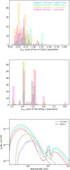 |
Fig. A.1 Same colour scheme as in Fig. 7. Top: Histogram of the wavelengths at the maximum of the polarised extinction curve of carbonaceous grains. Centre: Same for the silicate grains. Bottom: Polarised extinction of the carbonaceous (dashed lines) and silicate grains (solid lines) for the best fits presented in Fig. 7. |
Figure A.1 shows the λmax of each carbonaceous and silicate grain populations for the models in Fig. 7. The carbonaceous grains make a non-negligible contribution in the near- to mid-IR, before the rise of the 10 µm-silicate feature. This is also seen in total extinction (Fig. A.3).
Figure A.2 presents the total and polarised SEDs per population of the best-fit models shown in Fig. 7. In the case of the total SED, the silicates always dominate in the far-IR, but the carbonaceous grains dominate in the millimetre range. The wavelength at which the transition occurs between the two populations depends on the exact composition of the grains, since this determines their spectral index. The results for the polarised SED are more mixed. In the four examples presented, corresponding to the four best models shown in Fig. 7, we observe that (i) the two normalised to the Bohlin’s ratio behave as for the total SED with a transition between silicates and carbonaceous grains from the far-IR to the millimetre range and that (ii) the two normalised to the Lenz’s ratio are dominated by the carbonaceous grains for the entire wavelength range. This is just an illustration of what the collection of acceptable models presented in Fig. 7 can produce. Indeed, for half of the models, the silicates dominate the polarised SED for both normalisations. The relative contributions of each population thus depend on two parameters: the choice made for the normalisation of the data and the exact composition of the grains.
As an example, Fig. A.4 shows the maximum grain alignment fraction ƒmax in the case of a normalisation to the Lenz’s ratio and pV/E(B − V) = 13%.mag−1. There is no correlation between the two parameters, regardless of whether the two populations are aligned in the same way or whether the carbonaceous grains and silicates obey two different alignment functions. Indeed, in addition to ƒmax, pV/E(B − V) depends on the grain chemical composition as well as their size distribution. This result was already visible in Guillet et al. (2018, see their Table 3).
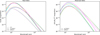 |
Fig. A.2 Same colour scheme as in Fig. 7. Contributions to the total and polarised SEDs of the nanometric hydrocarbons a-C shown by the dotted lines, of the a-C:H/a-C grains by the dashed lines and of the silicates by the solid lines. Left: Total SEDs of the best-fit models presented in Fig. 7. Right: Corresponding polarised SEDs. |
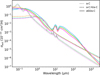 |
Fig. A.3 Same colour scheme as in Fig. 7. Contributions to the total extinction of the nanometric hydrocarbons a-C shown by the dotted lines, of the a-C:H/a-C grains by the dashed lines and of the silicates by the solid lines. |
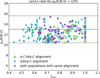 |
Fig. A.4 Maximum grain alignment fraction ƒmax in the case of a normalisation to the Lenz’s ratio for pV/E(B − V) = 13%.mag−1 (black line and ±20% uncertainty as dashed lines). Model results are shown for the case of a universal alignment function for both grain populations (pink circles) and for different alignment functions for carbonaceous and silicate grains shown as yellow squares and green diamonds, respectively. |
Appendix B Deviation of the model from the total and polarised observed SEDs
 |
Fig. B.1 Deviation of the four best models presented in Fig. 7 for the total (left) and polarised (right) SEDs. Same colour scheme as in Fig. 7. For clarity, the wavelengths are shifted by a few percents for the points not to overlap too much. |
Figure B.1 shows the deviation of the four best models presented in Fig. 7 from the total and polarised SEDs. This shows an agreement within ±20% at almost all wavelengths which is the precision requirement we adopted following Hensley & Draine (2023).
Appendix C Fits with THEMIS I silicates
Here we present the results obtained if instead of using the latest laboratory results for silicates (Demyk et al. 2017, 2022) we use the old silicates from the first version of THEMIS (Jones et al. 2013; Köhler et al. 2014). The grain shapes and elongations, as well as the compositions of the carbonaceous grains explored, are the same as those used in the rest of the paper.
Figure C.4 is the counterpart to Fig. 7, Fig. C.1 to Fig. 8, Fig. C.2 to Fig. 9, Fig. C.3 to Fig. 10, and Fig. C.5 to Fig. 11. Regardless of the normalisation chosen for the observations, it is always possible to find acceptable agreement between them and the model (Fig C.4). The best fits are obtained for:
THEMIS I silicates (oblates, e = 1.3) and a-CH/a-C5nm (oblates, e = 2) in the case of a normalisation to the Bohlin’s ratio and for pV/E(B − V) = 9%
THEMIS I silicates (prolates, e = 1.3) and a-CH/a-C5nm (oblates, e = 2) in the case of a normalisation to the Bohlin’s ratio and for pV/E(B − V) = 13%
THEMIS I silicates (oblates, e = 1.3) and a-CH/a-C5nm (prolates, e = 2) in the case of a normalisation to the Lenz’s ratio and for pV/E(B − V) = 9%
THEMIS I silicates (prolates, e = 2) and a-CH/a-C5nm (prolates, e = 2) in the case of a normalisation to the Lenz’s ratio and for pV/E(B − V) = 13%.
In the same way as with the silicates derived from the laboratory data, all shapes and elongations give acceptable fits with observations and most models require only imperfect grain alignment. The polarisation fraction at 3.4 µm is also compatible with the upper limits measured towards the Galactic Centre (Fig. C.1 Chiar & Tielens 2006).
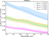 |
Fig. C.1 Same as in Fig. 8 but for fits performed with THEMIS I silicates (see Table 1). Same colour scheme as in Fig. C.4. |
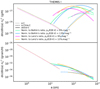 |
Fig. C.2 Same as Fig. 9 but for fits performed with THEMIS I silicates (see Table 1). Same colour scheme as in Fig. C.4. |
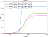 |
Fig. C.3 Same as Fig. 10 but for fits performed with THEMIS I silicates (see Table 1). Same colour scheme as in Fig. C.4. |
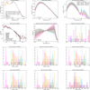 |
Fig. C.4 Same as Fig. 7 but for fits performed with THEMIS I silicates (see Table 1). The data are those presented in Sect. 5. From top to bottom and left to right, the figures first show the models against the observations: total SED, polarised SED, polarised extinction, total extinction; and then some model parameters: radiation field, silicium abundance, magnesium abundance, oxygen abundance, iron abundance, sulphur abundance, and carbon abundance. The light coloured areas represent the dispersion of the models in agrement with the observations and the matching thick solid lines show the best fits. As detailed in the text, two gas-to-dust mass ratios and two maximum optical polarisation values are considered to normalise the models. The models normalised to the ratio of Lenz et al. (2017) are shown in magenta and orange for pV/E(B − V) = 9% and 13%, respectively. Those normalised to the ratio of Bohlin et al. (1978) are shown in green and blue for pV/E(B − V) = 9% and 13%, respectively. |
Finally, Fig. C.5 shows how models using the THEMIS I silicates compare with the dust parameters derived by Planck Collaboration XI (2014) for the diffuse ISM. Even if the collection of acceptable models are compatible with the tendencies measured by Planck Collaboration XI (2014), it cannot explain the whole dispersion in the observations. This illustrates the need for diversity in the chemical composition of silicates to reconcile dust models and dust observations.
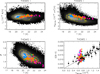 |
Fig. C.5 Same as Fig. 11 but for fits performed with THEMIS I silicates (see Table 1). Variations in the dust parameters presented by Planck Collaboration XI (2014), based on a pixel-by-pixel modified blackbody χ2-fit. In the top left and right, and the bottom left figures, the observational results are the density of points maps, on which we overplot yellow contours: the central contour encloses 50% of the observed pixels and the external contour 75%. In the bottom right figure, the observational results are the black dots with error bars. In the four figures, the model results are the coloured dots, with the same colour scheme as in Fig. C.4. Models normalised to the ratio of Lenz et al. (2017) are shown by magenta and orange dots for pV/E(B − V) = 9% and 13%, respectively. Those normalised to the ratio of Bohlin et al. (1978) are shown by green and blue dots for pV/E(B − V) = 9% and 13%, respectively. Top left: Luminosity vs temperature. Top right: Opacity at 353 GHz vs temperature. Bottom left: Spectral index vs temperature. Bottom right: E(B-V) vs optical depth at 353 GHz, models shown for NH = 1020 H/cm2. |
References
- Adamson, A. J., Whittet, D. C. B., Chrysostomou, A., et al. 1999, ApJ, 512, 224 [NASA ADS] [CrossRef] [Google Scholar]
- Agladze, N. I., Sievers, A. J., Jones, S. A., Burlitch, J. M., & Beckwith, S. V. W. 1996, ApJ, 462, 1026 [NASA ADS] [CrossRef] [Google Scholar]
- Akhukov, M. A., Katsnelson, M. I., & Fasolino, A. 2013, J. Phys. Condensed Matter, 25, 255301 [CrossRef] [Google Scholar]
- Andersson, B. G., Lazarian, A., & Vaillancourt, J. E. 2015, ARA&A, 53, 501 [Google Scholar]
- Angarita, Y., Versteeg, M. J. F., Haverkorn, M., et al. 2023, AJ, 166, 34 [NASA ADS] [CrossRef] [Google Scholar]
- Ashton, P. C., Ade, P. A. R., Angilè, F. E., et al. 2018, ApJ, 857, 10 [Google Scholar]
- Bedell, M., Bean, J. L., Meléndez, J., et al. 2018, ApJ, 865, 68 [Google Scholar]
- Bianchi, S., Giovanardi, C., Smith, M. W. L., et al. 2017, A&A, 597, A130 [NASA ADS] [CrossRef] [EDP Sciences] [Google Scholar]
- Binet, L., Gourier, D., Derenne, S., & Robert, F. 2002, Geochim. Cos-mochim. Acta, 66, 4177 [CrossRef] [Google Scholar]
- Binet, L., Gourier, D., Derenne, S., Robert, F., & Ciofini, I. 2004, Geochim. Cos-mochim. Acta, 68, 881 [CrossRef] [Google Scholar]
- Bohlin, R. C., Savage, B. D., & Drake, J. F. 1978, ApJ, 224, 132 [Google Scholar]
- Bohren, C., & Huffman, D. 1983, Absorption and Scattering of Light by Small Particles (New York – Chichester – Brisbane – Toronto – Singapore: Wiley and Sons) [Google Scholar]
- Boudet, N., Mutschke, H., Nayral, C., et al. 2005, ApJ, 633, 272 [Google Scholar]
- Cardelli, J. A., Clayton, G. C., & Mathis, J. S. 1989, ApJ, 345, 245 [Google Scholar]
- Chapman, N. L., Mundy, L. G., Lai, S.-P., & Evans, Neal J., I. 2009, ApJ, 690, 496 [NASA ADS] [CrossRef] [Google Scholar]
- Chen, X., Wang, S., Deng, L., & de Grijs, R. 2018, ApJ, 859, 137 [NASA ADS] [CrossRef] [Google Scholar]
- Chiar, J. E., & Tielens, A. G. G. M. 2006, ApJ, 637, 774 [NASA ADS] [CrossRef] [Google Scholar]
- Compiègne, M., Verstraete, L., Jones, A., et al. 2011, A&A, 525, A103 [Google Scholar]
- Costantini, E., Freyberg, M. J., & Predehl, P. 2005, A&A, 444, 187 [NASA ADS] [CrossRef] [EDP Sciences] [Google Scholar]
- Costantini, E., Pinto, C., Kaastra, J. S., et al. 2012, A&A, 539, A32 [NASA ADS] [CrossRef] [EDP Sciences] [Google Scholar]
- Coupeaud, A., Demyk, K., Meny, C., et al. 2011, A&A, 535, A124 [NASA ADS] [CrossRef] [EDP Sciences] [Google Scholar]
- Das, H. K., Voshchinnikov, N. V., & Il’in, V. B. 2010, MNRAS, 404, 265 [NASA ADS] [Google Scholar]
- Davidson, J., Nittler, L. R., Stroud, R. M., et al. 2015, in 46th Annual Lunar and Planetary Science Conference, Lunar and Planetary Science Conference, 1609 [Google Scholar]
- Davoisne, C., Djouadi, Z., Leroux, H., et al. 2006, A&A, 448, L1 [NASA ADS] [CrossRef] [EDP Sciences] [Google Scholar]
- De Cia, A., Jenkins, E. B., Fox, A. J., et al. 2021, Nature, 597, 206 [NASA ADS] [CrossRef] [Google Scholar]
- Decleir, M., Gordon, K. D., Andrews, J. E., et al. 2022, ApJ, 930, 15 [NASA ADS] [CrossRef] [Google Scholar]
- Delpoux, O. 2009, PhD Thesis, Chimie ParisTech, France [Google Scholar]
- Demyk, K., Carrez, P., Leroux, H., et al. 2001, A&A, 368, L38 [NASA ADS] [CrossRef] [EDP Sciences] [Google Scholar]
- Demyk, K., Meny, C., Lu, X. H., et al. 2017, A&A, 237, 215 [Google Scholar]
- Demyk, K., Gromov, V., Meny, C., et al. 2022, A&A, 666, A192 [NASA ADS] [CrossRef] [EDP Sciences] [Google Scholar]
- Désert, F. X., Boulanger, F., & Puget, J. L. 1990, A&A, 500, 313 [Google Scholar]
- Djouadi, Z., Gattacceca, J., D'Hendecourt, L., et al. 2007, A&A, 468, L9 [NASA ADS] [CrossRef] [EDP Sciences] [Google Scholar]
- Draine, B. T., & Flatau, P. J. 1994, J. Opt. Soc. Am. A, 11, 1491 [NASA ADS] [CrossRef] [Google Scholar]
- Draine, B. T., & Flatau, P. J. 2008, J. Opt. Soc. Am. A, 25, 2693 [NASA ADS] [CrossRef] [Google Scholar]
- Draine, B. T., & Flatau, P. J. 2013, arXiv e-prints [arXiv:1305.6497] [Google Scholar]
- Draine, B. T., & Fraisse, A. A. 2009, ApJ, 696, 1 [Google Scholar]
- Draine, B. T., & Hensley, B. S. 2021a, ApJ, 910, 47 [NASA ADS] [CrossRef] [Google Scholar]
- Draine, B. T., & Hensley, B. S. 2021b, ApJ, 909, 94 [NASA ADS] [CrossRef] [Google Scholar]
- Draine, B. T., & Hensley, B. S. 2021c, ApJ, 919, 65 [NASA ADS] [CrossRef] [Google Scholar]
- Draine, B. T., & Lee, H. M. 1984, ApJ, 285, 89 [NASA ADS] [CrossRef] [Google Scholar]
- Draine, B. T., & Li, A. 2007, ApJ, 657, 810 [CrossRef] [Google Scholar]
- Dwek, E., Arendt, R. G., Fixsen, D. J., et al. 1997, ApJ, 475, 565 [NASA ADS] [CrossRef] [Google Scholar]
- Esquinazi, P., & Höhne, R. 2005, J. Magn. Magn. Mater., 290, 20 [CrossRef] [Google Scholar]
- Fanciullo, L., Guillet, V., Aniano, G., et al. 2015, A&A, 580, A136 [NASA ADS] [CrossRef] [EDP Sciences] [Google Scholar]
- Fanciullo, L., Guillet, V., Boulanger, F., & Jones, A. P. 2017, A&A, 602, A7 [NASA ADS] [CrossRef] [EDP Sciences] [Google Scholar]
- Fitzpatrick, E. L., Massa, D., Gordon, K. D., Bohlin, R., & Clayton, G. C. 2019, ApJ, 886, 108 [Google Scholar]
- Flatau, P. J., & Draine, B. T. 2012, Opt. Express, 20, 1247 [NASA ADS] [CrossRef] [Google Scholar]
- Gao, J., Jiang, B. W., & Li, A. 2009, ApJ, 707, 89 [NASA ADS] [CrossRef] [Google Scholar]
- Gordon, K. D., Cartledge, S., & Clayton, G. C. 2009, ApJ, 705, 1320 [NASA ADS] [CrossRef] [Google Scholar]
- Gordon, K. D., Misselt, K. A., Bouwman, J., et al. 2021, ApJ, 916, 33 [NASA ADS] [CrossRef] [Google Scholar]
- Gordon, K. D., Clayton, G. C., Decleir, M., et al. 2023, ApJ, 950, 86 [CrossRef] [Google Scholar]
- Goto, M., Maihara, T., Terada, H., et al. 2000, A&AS, 141, 149 [NASA ADS] [CrossRef] [EDP Sciences] [Google Scholar]
- Goto, M., Kwok, S., Takami, H., et al. 2007, ApJ, 662, 389 [NASA ADS] [CrossRef] [Google Scholar]
- Guillet, V., Fanciullo, L., Verstraete, L., et al. 2018, A&A, 610, A16 [NASA ADS] [CrossRef] [EDP Sciences] [Google Scholar]
- Hensley, B. S., & Draine, B. T. 2020, ApJ, 895, 38 [NASA ADS] [CrossRef] [Google Scholar]
- Hensley, B. S., & Draine, B. T. 2021, ApJ, 906, 73 [NASA ADS] [CrossRef] [Google Scholar]
- Hensley, B. S., & Draine, B. T. 2023, ApJ, 948, 55 [Google Scholar]
- Hoang, T., & Lazarian, A. 2016, ApJ, 831, 159 [Google Scholar]
- Hoang, T., Minh Phan, V. H., & Tram, L. N. 2023, ApJ, 954, 216 [CrossRef] [Google Scholar]
- Hong, S. S., & Greenberg, J. M. 1980, A&A, 88, 194 [NASA ADS] [Google Scholar]
- Hoppe, P., Leitner, J., & Kodolányi, J. 2018, ApJ, 869, 47 [NASA ADS] [CrossRef] [Google Scholar]
- Hoppe, P., Leitner, J., Kodolányi, J., Borrmann, S., & Jones, A. P. 2022, Nat. Astron., 6, 1027 [Google Scholar]
- Indebetouw, R., Mathis, J. S., Babler, B. L., et al. 2005, ApJ, 619, 931 [NASA ADS] [CrossRef] [Google Scholar]
- Ingalls, J. G., Bania, T. M., Boulanger, F., et al. 2011, ApJ, 743, 174 [NASA ADS] [CrossRef] [Google Scholar]
- Ishii, M., Nagata, T., Chrysostomou, A., & Hough, J. H. 2002, AJ, 124, 2790 [NASA ADS] [CrossRef] [Google Scholar]
- Ishii, H. A., Bradley, J. P., Bechtel, H. A., et al. 2018, PNAS, 115, 6608 [NASA ADS] [CrossRef] [Google Scholar]
- Jäger, C., Sabri, T., Wendler, E., & Henning, T. 2016, ApJ, 831, 66 [CrossRef] [Google Scholar]
- Jenkins, E. B. 2009, ApJ, 700, 1299 [Google Scholar]
- Jones, A. P. 2012a, A&A, 540, A1 [NASA ADS] [CrossRef] [EDP Sciences] [Google Scholar]
- Jones, A. P. 2012b, A&A, 540, A2 [NASA ADS] [CrossRef] [EDP Sciences] [Google Scholar]
- Jones, A. P. 2012c, A&A, 542, A98 [NASA ADS] [CrossRef] [EDP Sciences] [Google Scholar]
- Jones, A. P. 2013, A&A, 555, A39 [NASA ADS] [CrossRef] [EDP Sciences] [Google Scholar]
- Jones, A. P. 2016, Roy. Soc. Open Sci., 3, 160224 [NASA ADS] [CrossRef] [Google Scholar]
- Jones, A. P., Fanciullo, L., Köhler, M., et al. 2013, A&A, 558, A62 [NASA ADS] [CrossRef] [EDP Sciences] [Google Scholar]
- Jones, A. P., Ysard, N., Köhler, M., et al. 2014, Faraday Discuss., 168, 313 [Google Scholar]
- Jones, A. P., Köhler, M., Ysard, N., et al. 2016, A&A, 588, A43 [NASA ADS] [CrossRef] [EDP Sciences] [Google Scholar]
- Jones, A. P., Köhler, M., Ysard, N., Bocchio, M., & Verstraete, L. 2017, A&A, 602, A46 [NASA ADS] [CrossRef] [EDP Sciences] [Google Scholar]
- Kemper, F., Vriend, W. J., & Tielens, A. G. G. M. 2004, ApJ, 609, 826 [Google Scholar]
- Köhler, M., Stepnik, B., Jones, A. P., et al. 2012, A&A, 548, A61 [NASA ADS] [CrossRef] [EDP Sciences] [Google Scholar]
- Köhler, M., Jones, A., & Ysard, N. 2014, A&A, 565, A9 [Google Scholar]
- Lai, T. S. Y., Smith, J. D. T., Baba, S., Spoon, H. W. W., & Imanishi, M. 2020, ApJ, 905, 55 [NASA ADS] [CrossRef] [Google Scholar]
- Lazarian, A. 2020, ApJ, 902, 97 [CrossRef] [Google Scholar]
- Lee, H. M., & Draine, B. T. 1985, ApJ, 290, 211 [Google Scholar]
- Lenz, D., Hensley, B. S., & Doré, O. 2017, ApJ, 846, 38 [NASA ADS] [CrossRef] [Google Scholar]
- Liszt, H. 2014, ApJ, 780, 10 [Google Scholar]
- Mason, R. E., Wright, G. S., Adamson, A., & Pendleton, Y. 2007, ApJ, 656, 798 [CrossRef] [Google Scholar]
- Massa, D., Fitzpatrick, E. L., & Gordon, K. D. 2020, ApJ, 891, 67 [NASA ADS] [CrossRef] [Google Scholar]
- Mathis, J. S., Mezger, P. G., & Panagia, N. 1983, A&A, 128, 212 [NASA ADS] [Google Scholar]
- McClure, M. 2009, ApJ, 693, L81 [NASA ADS] [CrossRef] [Google Scholar]
- McMillan, R. S., & Tapia, S. 1977, ApJ, 212, 714 [NASA ADS] [CrossRef] [Google Scholar]
- Mennella, V., Brucato, J. R., Colangeli, L., et al. 1998, ApJ, 496, 1058 [NASA ADS] [CrossRef] [Google Scholar]
- Min, M., Waters, L. B. F. M., de Koter, A., et al. 2007, A&A, 462, 667 [NASA ADS] [CrossRef] [EDP Sciences] [Google Scholar]
- Mishchenko, M. I., & Yurkin, M. A. 2017, Opt. Lett., 42, 494 [NASA ADS] [CrossRef] [Google Scholar]
- Mishra, A., & Li, A. 2017, ApJ, 850, 138 [NASA ADS] [CrossRef] [Google Scholar]
- Murray, C. E., Peek, J. E. G., Lee, M.-Y., & Stanimirovic, S. 2018, ApJ, 862, 131 [NASA ADS] [CrossRef] [Google Scholar]
- Nagatomo, S., Nagata, T., & Nishiyama, S. 2019, PASJ, 71, 106 [NASA ADS] [CrossRef] [Google Scholar]
- Nguyen, H., Dawson, J. R., Miville-Deschênes, M. A., et al. 2018, ApJ, 862, 49 [NASA ADS] [CrossRef] [Google Scholar]
- Nieva, M. F., & Przybilla, N. 2012, A&A, 539, A143 [NASA ADS] [CrossRef] [EDP Sciences] [Google Scholar]
- Nishiyama, S., Nagata, T., Kusakabe, N., et al. 2006, ApJ, 638, 839 [Google Scholar]
- Nishiyama, S., Tamura, M., Hatano, H., et al. 2009, ApJ, 696, 1407 [NASA ADS] [CrossRef] [Google Scholar]
- Ordal, M. A., Bell, R. J., Alexander, R. W., J., Long, L. L., & Querry, M. R. 1985, Appl. Opt., 24, 4493 [NASA ADS] [CrossRef] [Google Scholar]
- Ordal, M. A., Bell, R. J., Alexander, Ralph W., J., Newquist, L. A., & Querry, M. R. 1988, Appl. Opt., 27, 1203 [NASA ADS] [CrossRef] [Google Scholar]
- Panopoulou, G. V., Hensley, B. S., Skalidis, R., Blinov, D., & Tassis, K. 2019, A&A, 624, L8 [NASA ADS] [CrossRef] [EDP Sciences] [Google Scholar]
- Parravano, A., Hollenbach, D. J., & McKee, C. F. 2003, ApJ, 584, 797 [Google Scholar]
- Parvathi, V. S., Sofia, U. J., Murthy, J., & Babu, B. R. S. 2012, ApJ, 760, 36 [NASA ADS] [CrossRef] [Google Scholar]
- Planck Collaboration XI. 2014, A&A, 571, A11 [NASA ADS] [CrossRef] [EDP Sciences] [Google Scholar]
- Planck Collaboration XI. 2020, A&A, 641, A11 [NASA ADS] [CrossRef] [EDP Sciences] [Google Scholar]
- Planck Collaboration XII. 2020, A&A, 641, A12 [NASA ADS] [CrossRef] [EDP Sciences] [Google Scholar]
- Planck Collaboration Int. XVII. 2014, A&A, 566, A55 [NASA ADS] [CrossRef] [EDP Sciences] [Google Scholar]
- Planck Collaboration Int. XXI. 2015, A&A, 576, A106 [NASA ADS] [CrossRef] [EDP Sciences] [Google Scholar]
- Planck Collaboration Int. XXII. 2015, A&A, 576, A107 [NASA ADS] [CrossRef] [EDP Sciences] [Google Scholar]
- Planck Collaboration Int. XXIX. 2016, A&A, 586, A132 [NASA ADS] [CrossRef] [EDP Sciences] [Google Scholar]
- Pollack, J. B., Hollenbach, D., Beckwith, S., et al. 1994, ApJ, 421, 615 [Google Scholar]
- Psaradaki, I., Costantini, E., Rogantini, D., et al. 2023, A&A, 670, A30 [NASA ADS] [CrossRef] [EDP Sciences] [Google Scholar]
- Purcell, E. M., & Pennypacker, C. R. 1973, ApJ, 186, 705 [NASA ADS] [CrossRef] [Google Scholar]
- Reach, W. T., Heiles, C., & Bernard, J.-P. 2015, ApJ, 811, 118 [NASA ADS] [CrossRef] [Google Scholar]
- Reach, W. T., Bernard, J.-P., Jarrett, T. H., & Heiles, C. 2017, ApJ, 851, 119 [NASA ADS] [CrossRef] [Google Scholar]
- Remy, Q., Grenier, I. A., Marshall, D. J., & Casandjian, J. M. 2018, A&A, 616, A71 [NASA ADS] [CrossRef] [EDP Sciences] [Google Scholar]
- Rieke, G. H., & Lebofsky, M. J. 1985, ApJ, 288, 618 [Google Scholar]
- Rogantini, D., Costantini, E., Zeegers, S. T., et al. 2019, A&A, 630, A143 [NASA ADS] [CrossRef] [EDP Sciences] [Google Scholar]
- Sakai, Y., Chelikowsky, J. R., & Cohen, M. L. 2018, Phys. Rev. Mater., 2, 074403 [NASA ADS] [CrossRef] [Google Scholar]
- Schlafly, E. F., Meisner, A. M., Stutz, A. M., et al. 2016, ApJ, 821, 78 [NASA ADS] [CrossRef] [Google Scholar]
- Schneider, D. P., Richards, G. T., Hall, P. B., et al. 2010, AJ, 139, 2360 [Google Scholar]
- Scott, A., & Duley, W. W. 1996, ApJS, 105, 401 [NASA ADS] [CrossRef] [Google Scholar]
- Serkowski, K., Mathewson, D. S., & Ford, V. L. 1975, ApJ, 196, 261 [NASA ADS] [CrossRef] [Google Scholar]
- Siebenmorgen, R. 2023, A&A, 670, A115 [NASA ADS] [CrossRef] [EDP Sciences] [Google Scholar]
- Siebenmorgen, R., Voshchinnikov, N. V., & Bagnulo, S. 2014, A&A, 561, A82 [NASA ADS] [CrossRef] [EDP Sciences] [Google Scholar]
- Siebenmorgen, R., Voshchinnikov, N. V., Bagnulo, S., et al. 2018, A&A, 611, A5 [NASA ADS] [CrossRef] [EDP Sciences] [Google Scholar]
- Siebenmorgen, R., Smoker, J., Krelowski, J., Gordon, K., & Chini, R. 2023, A&A, 676, A132 [NASA ADS] [CrossRef] [EDP Sciences] [Google Scholar]
- Sofia, U. J., & Meyer, D. M. 2001, ApJ, 554, L221 [Google Scholar]
- Sofia, U. J., Parvathi, V. S., Babu, B. R. S., & Murthy, J. 2011, AJ, 141, 22 [NASA ADS] [CrossRef] [Google Scholar]
- Tamor, M. A., & Wu, C. H. 1990, J. Appl. Phys., 67, 1007 [NASA ADS] [CrossRef] [Google Scholar]
- Telesco, C. M., Varosi, F., Wright, C., et al. 2022, ApJ, 940, L26 [NASA ADS] [CrossRef] [Google Scholar]
- Vaillancourt, J. E., Andersson, B. G., Clemens, D. P., et al. 2020, ApJ, 905, 157 [NASA ADS] [CrossRef] [Google Scholar]
- van Breemen, J. M., Min, M., Chiar, J. E., et al. 2011, A&A, 526, A152 [NASA ADS] [CrossRef] [EDP Sciences] [Google Scholar]
- Van De Putte, D., Cartledge, S. I. B., Gordon, K. D., Clayton, G. C., & Roman-Duval, J. 2023, ApJ, 944, 33 [NASA ADS] [CrossRef] [Google Scholar]
- Voshchinnikov, N. V., & Henning, T. 2010, A&A, 517, A45 [NASA ADS] [CrossRef] [EDP Sciences] [Google Scholar]
- Voshchinnikov, N. V., Il’in, V. B., & Das, H. K. 2016, MNRAS, 462, 2343 [NASA ADS] [CrossRef] [Google Scholar]
- Wang, S., & Chen, X. 2019, ApJ, 877, 116 [Google Scholar]
- Wang, S., Gao, J., Jiang, B. W., Li, A., & Chen, Y. 2013, ApJ, 773, 30 [NASA ADS] [CrossRef] [Google Scholar]
- Wang, S., Li, A., & Jiang, B. W. 2015, ApJ, 811, 38 [NASA ADS] [CrossRef] [Google Scholar]
- Weingartner, J. C., & Draine, B. T. 2001, ApJ, 548, 296 [Google Scholar]
- Xiang, J., Lee, J. C., Nowak, M. A., & Wilms, J. 2011, ApJ, 738, 78 [Google Scholar]
- Xue, M., Jiang, B. W., Gao, J., et al. 2016, Apjs, 224, 23 [NASA ADS] [CrossRef] [Google Scholar]
- Ysard, N. 2020, in Laboratory Astrophysics: From Observations to Interpretation, eds. F. Salama, & H. Linnartz, 350, 53 [NASA ADS] [Google Scholar]
- Ysard, N., Abergel, A., Ristorcelli, I., et al. 2013, A&A, 559, A133 [NASA ADS] [CrossRef] [EDP Sciences] [Google Scholar]
- Ysard, N., Köhler, M., Jones, A., et al. 2015, A&A, 577, A110 [NASA ADS] [CrossRef] [EDP Sciences] [Google Scholar]
- Ysard, N., Jones, A. P., Demyk, K., Boutéraon, T., & Koehler, M. 2018, A&A, 617, A124 [NASA ADS] [CrossRef] [EDP Sciences] [Google Scholar]
- Ysard, N., Koehler, M., Jimenez-Serra, I., Jones, A. P., & Verstraete, L. 2019, A&A, 631, A88 [NASA ADS] [CrossRef] [EDP Sciences] [Google Scholar]
- Ysard, N., Miville-Deschênes, M. A., Verstraete, L., & Jones, A. P. 2022, A&A, 663, A65 [NASA ADS] [CrossRef] [EDP Sciences] [Google Scholar]
- Zeegers, S. T., Costantini, E., de Vries, C. P., et al. 2017, A&A, 599, A117 [NASA ADS] [CrossRef] [EDP Sciences] [Google Scholar]
- Zeegers, S. T., Costantini, E., Rogantini, D., et al. 2019, A&A, 627, A16 [NASA ADS] [CrossRef] [EDP Sciences] [Google Scholar]
- Zuo, W., Li, A., & Zhao, G. 2021, ApJS, 257, 63 [NASA ADS] [CrossRef] [Google Scholar]
Their ‘astrodust’ model is fully characterised in Draine & Hensley (2021a,b,c).
Available here: https://www.ias.u-psud.fr/themis/
This core-mantle structure is in agreement with observations of primitive chondrites (Ishii et al. 2018) and GEMS (glass with embedded metal and sulfides) inside interplanetary dust particles (Davidson et al. 2015).
Forsterite is a mineral of the silicate group and the mesosilicate subgroup. With a composition of Mg2SiO4, it is the pure magnesian end member of olivine. Enstatite is a mineral species in the silicate subgroup of inosilicates. It is a member of the pyroxene family, with the formula MgSiO3. When we talk of forsterite, olivine, enstatite or pyroxene in an amorphous state what we implicitly imply is silicates that have these stoichiometries and not the crystalline silicates to which these mineralogical terms apply.
For a complete presentation of the different samples measured by Demyk et al. (2017), including iron-rich silicates, see Demyk et al. (2022). See also the study by Siebenmorgen (2023) for their effects when used in dust models.
Available here: https://www.ias.u-psud.fr/DUSTEM/
As per the original version, THEMIS 2.0 is constructed to model the dust in the low density, diffuse ISM, we therefore do not consider porous grains (vacuum inclusions).
As no changes are made to the properties of the carbonaceous nano-grains, the spectroscopic predictions presented in our previous studies for denser/brighter regions remain valid (e.g. Jones 2012c; Jones et al. 2013, 2016). Similarly, the microwave spinning dust emission is not affected by the update that we make here and the conclusions of Ysard et al. (2022) still hold for THEMIS 2.0.
Gordon et al. (2023) carried out such a study from the UV to mid-IR using the samples of Gordon et al. (2009, 2021), Fitzpatrick et al. (2019), and Decleir et al. (2022). However, to produce an average extinction curve, they use observations of lines of sight with A(V) ≳ 4 which results in a higher mid-IR band-to-continuum ratio.
We can also illustrate this in terms of RV : the Bohlin normalisation is equivalent to the Lenz normalisation if we decrease the value of RV from 3.1 to 2.1, for example. This exploration should therefore lead to a dispersion of the value of RV in the models in line with the measurements presented in Sect. 5.4.
Scaling factor for the radiation field integrated between 6 and 13.6 eV. The standard ISRF corresponds to G0 = 1 and to a flux of 1.6 × 10⁻³ erg s−1 cm−2 (Parravano et al. 2003).
Available here: http://dustemwrap.irap.omp.eu/Home.html
The Planck-HFI data showed that the dust is probably different in the Galactic plane, where a higher spectral index is observed than at higher latitudes, and that this spectral index is correlated with temperature, unlike in the high-latitude sky where these two quantities are anti-correlated (see for instance Planck Collaboration XI 2014, and references therein).
Accessible here: https://www.ias.u-psud.fr/themis/
All Tables
Main parameters defining the best dust model normalised to the Lenz’s ratio and pV/E(B − V) = 13%mag-1 as in Siebenmorgen (2023) and Hensley & Draine (2023).
All Figures
|
Fig. 1 Complex refractive indices, m = n + ik, of the silicate materials. Top: real part. Bottom: imaginary part. Left: complex refractive indices for the calculation of the silicate grain optical properties. Demyk et al. (2017) silicate samples measured at 10 K are shown: forsterite X35 sample (black), enstatite X50a sample (light pink), enstatite X50b sample (light blue) along with the aSil-1, aSil-2, aSil-3, and aSil-4 mixtures as pink, blue, green, and yellow thick lines, respectively (see Sect. 2.1.2 and Table 1 for details). We note that 10% of the silicate volume is occupied by metallic nano-inclusions of Fe and FeS (70% and 30% of the total volume of the inclusions, respectively), hence the increase in the visible to mid-IR imaginary part of the refractive index. For comparison, the optical constants of the two silicate materials used in the original THEMIS are shown with dotted lines. The optical constants used for the 5 nm-thick aromatic-rich carbon mantles, a-C2.5nm, are also plotted (grey, see Sect. 2.2 for details). Right: same for the aSil-5, a-Sil-6, and aSil-7 mixtures as red, brown, and orange thick lines, respectively. |
| In the text | |
|
Fig. 2 Complex refractive indices, m = n + ik, for the calculation of the carbonaceous grain optical properties with those used for the mantle in grey (2.5 nm a-C), brown (4 nm a-C), orange (5 nm a-C), green (6 nm a-C), and blue (10 nm a-C) and the example of a 100 nm a-CH core in red. Top: real part. Bottom: imaginary part. |
| In the text | |
|
Fig. 3 Dependence of optical properties on grain shape (left) and size (right) for silicate grains made of aSil-1/a-C2.5nm materials (top) and carbonaceous grains with a-CH/a-C10nm composition (bottom). Each block of figures presents the total absorption and scattering efficiencies as solid and dashed lines (upper figure), respectively, and the polarisation efficiency Qpol = (β2,ext − β1,ext)/2 (lower figure). For comparison, Qpol for THEMIS I oblate silicates with e = 1.3 and variable size are shown in the lower figure of the top right block. |
| In the text | |
|
Fig. 4 Dependence of optical properties on grain composition for carbonaceous grains with a-CH/a-C2.5nm, a-CH/a-C4nm, a-CH/a-C5nm, a-CH/a-C6nm, and a-CH/a-C10nm compositions in grey, brown, orange, green, and blue, respetively (aeff = 100 nm, oblate with e = 1.3). Solid lines show Qabs and dashed lines Qsca. |
| In the text | |
|
Fig. 5 Dependence of optical properties on grain composition for silicate grains with cores made of aSil-1, aSil-2, aSil-3, and aSil-4 materials in pink, blue, green, and yellow, respectively (aeff = 100 nm, oblate with e = 1.3) on the left and cores made of aSil-5, aSil-6, and aSil-7 in red, brown, and orange, respectively, on the right. Top: solid lines show Qabs and dashed lines Qsca. Middle: zoom in on the silicate mid-IR features. Bottom: ratios of Qabs to THEMIS I. |
| In the text | |
|
Fig. 6 Core-mantle spheroidal grain volume densities. The blue line shows the case of grains with silicate cores with 5 nm-thick a-C mantles and the black line of a-C:H cores with 20 nm-thick a-C mantles. The thickness of the lines shows the little dispersion of the density as a function of the grain shape, oblate or prolate, and elongation. |
| In the text | |
|
Fig. 7 Data are those presented in Sect. 5. From top to bottom and left to right, the figures first show the models against the observations: total SED, polarised SED, polarised extinction, total extinction; and then some model parameters: radiation field, silicon abundance, magnesium abundance, oxygen abundance, iron abundance, sulphur abundance, and carbon abundance. The light coloured areas represent the dispersion of the models in agreement with the observations and the matching thick solid lines show the best fits (see Sect. 6.3 for details). As detailed in the text, two gas-to-dust mass ratios and two maximum optical polarisation values are considered to normalise the models. The models normalised to the ratio of Lenz et al. (2017) are shown in magenta and orange for pV/E(B − V) = 9% and 13%, respectively. Those normalised to the ratio of Bohlin et al. (1978) are shown in green and blue for pV/E(B − V) = 9% and 13%, respectively. |
| In the text | |
|
Fig. 8 Same colour scheme as in Fig. 7. Zoom on the 3.4 µm hydrocarbon feature seen in polarised extinction. The dashed lines show the upper limits measured by Chiar & Tielens (2006) towards GCS 3-II and GCS 3-IV, lowest and highest lines, respectively, above the continuum of our four best-fit models (see Sect. 6.3 for details). For comparison, we also show in grey the model of Hensley & Draine (2023) which complies with the upper limit measured towards GCS 3-IV but not with the lower one towards GCS 3-II. Hensley & Draine (2023) gives indeed ∆p3.4 µm 2 to 2.6 times as large as our best models. |
| In the text | |
|
Fig. 9 Same colour scheme as in Fig. 7. Top: grain mass distributions of the best-fit models shown in Fig. 7. Bottom: equivalent grain number distributions. In both figures, the distributions for the amorphous nano-carbon grains, a-C, are shown as dotted lines, for the a-C:H/a-C grains as dashed lines and for the aSil/a-C grains as solid lines. |
| In the text | |
|
Fig. 10 Alignment functions of the best fits presented in Fig. 7 and Sect. 6.3. The colour scheme is the same as in Fig. 7. Models normalised to the ratio of Lenz et al. (2017) are shown by magenta and orange lines for pV/E(B − V) = 9% and 13%, respectively. Both models are for pro-lates with e = 2. Those normalised to the ratio of Bohlin et al. (1978) are shown by green and blue lines for pV/E(B − V) = 9% and 13%, respectively. The model plotted in green is for oblates with e = 1.3 and the one in blue for prolates with e = 2. |
| In the text | |
|
Fig. 11 Variations in the dust parameters presented by Planck Collaboration XI (2014), based on a pixel-by-pixel modified blackbody χ2 fit (see Eq. (7) and Sect. 6.4 for details). In the top left and right, and the bottom left figures, the observational results are the density of points maps, on which we overplot yellow contours: the central contour encloses 50% of the observed pixels and the external contour 75%. In the bottom right figure, the observational results are the black dots with error bars. In the four figures, the model results are the coloured dots, with the same colour scheme as in Fig. 7. Models normalised to the ratio of Lenz et al. (2017) are shown by magenta and orange dots for pV/E(B − V) = 9% and 13%, respectively. Those normalised to the ratio of Bohlin et al. (1978) are shown by green and blue dots for pV/E(B − V) = 9% and 13%, respectively. For comparison, the dark blue squares show the parameters derived from the model of Hensley & Draine (2023). Top left: luminosity vs. temperature. Top right: opacity at 353 GHz vs. temperature. Bottom left: spectral index vs. temperature. Bottom right: E(B-V) vs. optical depth at 353 GHz, models shown for NH = 1020 H cm−2. |
| In the text | |
|
Fig. 12 Histograms of parameters derived from our best fits represented with the same colour scheme as in Fig. 7. For comparison, the parameters derived from the model of Hensley & Draine (2023) are shown by the dark blue squares. The two figures in the top row show two characteristic ratios of the polarised observations made with the Planck satellite: RP/p and RS/V. The measurements, including their uncertainties, made by Panopoulou et al. (2019) and Planck Collaboration XII (2020), are represented by the black horizontal lines. The two figures in the middle row show the dispersion of λmax (left) and of the polarised extinction at 10 µm normalised to the optical (right) of our best fits. The measurements, including their uncertainties, made by Vaillancourt et al. (2020) and Telesco et al. (2022) combined to McMillan & Tapia (1977) are shown by the black horizontal lines. The bottom row figure shows the histogram of the extinction parameter RV. The measurements made by Decleir et al. (2022), including their uncertainties, are shown by the black horizontal line. |
| In the text | |
|
Fig. A.1 Same colour scheme as in Fig. 7. Top: Histogram of the wavelengths at the maximum of the polarised extinction curve of carbonaceous grains. Centre: Same for the silicate grains. Bottom: Polarised extinction of the carbonaceous (dashed lines) and silicate grains (solid lines) for the best fits presented in Fig. 7. |
| In the text | |
|
Fig. A.2 Same colour scheme as in Fig. 7. Contributions to the total and polarised SEDs of the nanometric hydrocarbons a-C shown by the dotted lines, of the a-C:H/a-C grains by the dashed lines and of the silicates by the solid lines. Left: Total SEDs of the best-fit models presented in Fig. 7. Right: Corresponding polarised SEDs. |
| In the text | |
|
Fig. A.3 Same colour scheme as in Fig. 7. Contributions to the total extinction of the nanometric hydrocarbons a-C shown by the dotted lines, of the a-C:H/a-C grains by the dashed lines and of the silicates by the solid lines. |
| In the text | |
|
Fig. A.4 Maximum grain alignment fraction ƒmax in the case of a normalisation to the Lenz’s ratio for pV/E(B − V) = 13%.mag−1 (black line and ±20% uncertainty as dashed lines). Model results are shown for the case of a universal alignment function for both grain populations (pink circles) and for different alignment functions for carbonaceous and silicate grains shown as yellow squares and green diamonds, respectively. |
| In the text | |
|
Fig. B.1 Deviation of the four best models presented in Fig. 7 for the total (left) and polarised (right) SEDs. Same colour scheme as in Fig. 7. For clarity, the wavelengths are shifted by a few percents for the points not to overlap too much. |
| In the text | |
|
Fig. C.1 Same as in Fig. 8 but for fits performed with THEMIS I silicates (see Table 1). Same colour scheme as in Fig. C.4. |
| In the text | |
|
Fig. C.2 Same as Fig. 9 but for fits performed with THEMIS I silicates (see Table 1). Same colour scheme as in Fig. C.4. |
| In the text | |
|
Fig. C.3 Same as Fig. 10 but for fits performed with THEMIS I silicates (see Table 1). Same colour scheme as in Fig. C.4. |
| In the text | |
|
Fig. C.4 Same as Fig. 7 but for fits performed with THEMIS I silicates (see Table 1). The data are those presented in Sect. 5. From top to bottom and left to right, the figures first show the models against the observations: total SED, polarised SED, polarised extinction, total extinction; and then some model parameters: radiation field, silicium abundance, magnesium abundance, oxygen abundance, iron abundance, sulphur abundance, and carbon abundance. The light coloured areas represent the dispersion of the models in agrement with the observations and the matching thick solid lines show the best fits. As detailed in the text, two gas-to-dust mass ratios and two maximum optical polarisation values are considered to normalise the models. The models normalised to the ratio of Lenz et al. (2017) are shown in magenta and orange for pV/E(B − V) = 9% and 13%, respectively. Those normalised to the ratio of Bohlin et al. (1978) are shown in green and blue for pV/E(B − V) = 9% and 13%, respectively. |
| In the text | |
|
Fig. C.5 Same as Fig. 11 but for fits performed with THEMIS I silicates (see Table 1). Variations in the dust parameters presented by Planck Collaboration XI (2014), based on a pixel-by-pixel modified blackbody χ2-fit. In the top left and right, and the bottom left figures, the observational results are the density of points maps, on which we overplot yellow contours: the central contour encloses 50% of the observed pixels and the external contour 75%. In the bottom right figure, the observational results are the black dots with error bars. In the four figures, the model results are the coloured dots, with the same colour scheme as in Fig. C.4. Models normalised to the ratio of Lenz et al. (2017) are shown by magenta and orange dots for pV/E(B − V) = 9% and 13%, respectively. Those normalised to the ratio of Bohlin et al. (1978) are shown by green and blue dots for pV/E(B − V) = 9% and 13%, respectively. Top left: Luminosity vs temperature. Top right: Opacity at 353 GHz vs temperature. Bottom left: Spectral index vs temperature. Bottom right: E(B-V) vs optical depth at 353 GHz, models shown for NH = 1020 H/cm2. |
| In the text | |
Current usage metrics show cumulative count of Article Views (full-text article views including HTML views, PDF and ePub downloads, according to the available data) and Abstracts Views on Vision4Press platform.
Data correspond to usage on the plateform after 2015. The current usage metrics is available 48-96 hours after online publication and is updated daily on week days.
Initial download of the metrics may take a while.