| Issue |
A&A
Volume 698, June 2025
|
|
|---|---|---|
| Article Number | A200 | |
| Number of page(s) | 14 | |
| Section | Interstellar and circumstellar matter | |
| DOI | https://doi.org/10.1051/0004-6361/202554575 | |
| Published online | 16 June 2025 | |
From small dust to micron-sized aggregates: The influence of structure and composition on the dust optical properties
1
Université Paris-Saclay, Université Paris Cité, CEA, CNRS, AIM,
91191
Gif-sur-Yvette,
France
2
IRAP, CNRS, Université de Toulouse,
9 avenue du Colonel Roche,
31028
Toulouse Cedex 4,
France
3
Université Paris-Saclay, CNRS, Institut d’Astrophysique Spatiale,
91405
Orsay,
France
4
Institute of Space Sciences (ICE), CSIC, Campus UAB, Carrer de Can Magrans s/n,
08193
Barcelona,
Spain
5
ICREA,
Pg. Lluís Companys 23,
Barcelona,
Spain
★ Corresponding author: marie-anne.carpine@cea.fr
Received:
17
March
2025
Accepted:
18
April
2025
Context. Models of astrophysical dust are key to understanding several physical processes, from the role of dust grains as cooling agents in the interstellar medium (ISM) to their evolution in dense circumstellar discs, explaining the occurrence of planetary systems around many stars. Currently, most models aim to provide optical properties for dust grains in the diffuse ISM, and many do not account properly for complexity in terms of composition and structure when dust is expected to evolve in dense astrophysical environments.
Aims. Our purpose is to investigate, with a pilot sample of micron-size dust grains, the influence of hypotheses made about the dust structure, porosity, and composition when computing the optical properties of grown dust grains. We aim to produce a groundwork for building comprehensive yet realistic optical properties that accurately represent dust grains as they are expected to evolve in the dense clouds, cores, and discs. We are especially interested in exploring these effects on the resulting optical properties in the infrared and millimetre domains, where observations of these objects are widely used to constrain the dust properties.
Methods. Starting from the small dust grains developed in the THEMIS 2.0 model, we used the discrete dipole approximation to compute the optical properties of 1 μm grains, varying the hypotheses made about their composition and structure. We looked at the dust scattering, emission, and extinction to isolate potential simplifications and unavoidable differences between grain structures.
Results. We note significant differences in the optical properties depending on the dust structure and composition. Both the dust structure and porosity influence the dust properties in infrared and millimetre ranges, demonstrating that dust aggregates cannot be correctly approximated by compact or porous spheres. In particular, we show that the dust emissivity index in the millimetre can vary with fixed grain size.
Conclusions. Our work sheds light on the importance of taking the dust structure and porosity into account when interpreting observations in astrophysical environments where dust grains may have evolved significantly. For example, measuring the dust sizes using the emissivity index from millimetre observations of the dust thermal emission is a good but degenerate tool, as we observe differences of up to 25% in the dust emissivity index with compact or aggregate grains, varying in composition and structure. Efforts in carrying out physical models of grain growth, for instance, are required to establish realistic constraints on the structure of grown dust grains, and will be used in the future to build realistic dust models for the dense ISM.
Key words: methods: numerical / protoplanetary disks / stars: formation / stars: protostars / dust, extinction / evolution
© The Authors 2025
 Open Access article, published by EDP Sciences, under the terms of the Creative Commons Attribution License (https://creativecommons.org/licenses/by/4.0), which permits unrestricted use, distribution, and reproduction in any medium, provided the original work is properly cited.
This article is published in open access under the Subscribe to Open model. Subscribe to A&A to support open access publication.
1 Introduction
Interstellar dust is of great influence in many astrophysical processes. The correct understanding and modelling of dust is undeniably necessary, whether it is to understand the formation of planetesimals (Birnstiel et al. 2016), the formation of complex molecules on their surfaces (Herbst 2021; Dulieu et al. 2010; Wakelam et al. 2017), or to correctly interpret astronomical observations using dust as a tracer, in most spectral ranges (Galliano et al. 2018). In terms of physical processes, dust plays a crucial role in the interstellar medium (ISM) evolution, especially in star-forming regions where it interacts with the molecular gas, but also becomes key to setting the coupling with the magnetic field in places where the ionisation fraction of the gas by cosmic rays is very low (Zhao et al. 2020; Maury et al. 2022), and is the core of heating and cooling processes. More importantly, dust grains constitute the building blocks of planet formation (see e.g. Testi et al. 2014, and references therein). From an observational point of view, dust represents a major tracer, and an unavoidable asset with which to probe the cold Universe. Dust optical properties impact light absorption, scattering, emission, and polarisation, and are used to estimate various physical properties such as the gas temperature, mass, and spatial distribution. Conversely, little is known about the microscopic properties of the astrophysical dust and inferring them from observations is also not straightforward. From the diffuse ISM where only the smallest submicronic grains are observed (Mathis et al. 1977; Hirashita & Nozawa 2013) to the circumstellar discs where kilometre-sized planetary bodies are formed (Keppler et al. 2018), dust grains are expected to undergo an evolution, in terms of size and structure, as they are incorporated into astrophysical environments of increasing gas density: if small ISM grains can be considered as compact spheres or spheroids, dust growth by ballistic aggregation implies that larger grains may naturally inherit an aggregated structure. While the evolution of small dust into large pebbles in discs has long been explored because of its direct impact on the formation of rocky planets (Birnstiel 2024; Testi et al. 2014; Teiser et al. 2025; Drążkowska et al. 2021), the early evolution of dust grains in the dense (n ~ 106 cm−3) star-forming material that makes up the pristine disc material is still largely unexplored (Priestley et al. 2021; Hirashita & Li 2013). However, recent studies suggest that micron-sized grains may be present in dense clouds (Pagani et al. 2010; Dartois et al. 2024), and that the material surrounding young protostars (protostellar envelopes) could host dust grains a few tens of microns in size (Galametz et al. 2019; Cacciapuoti et al. 2023). Moreover, fractal aggregates and irregular solid grains have been observed in cometary dust in the Solar System, and are consistent with models of early dust aggregation from pristine material, in the solar nebula (e.g. Fulle & Blum 2017). Efforts to model complex dust particles should therefore be made not only to describe dust evolution towards planetary systems in discs, but also to interpret dust observations in dense clouds, cores, and protostellar envelopes. It is thus key to build realistic models of micron-sized grains to interpret the dust observations in such environments, and to ensure that these dust models are physically motivated by (i) constraints on dust properties in the diffuse ISM and (ii) predictions from dust growth models.
A dust model is first defined from the dust optical properties, which translate into the absorption, scattering, and extinction efficiencies of the dust grains (respectively Qabs, Qsca and Qext, extensively defined in Bohren & Huffman 1983), tabulated by wavelength and grain size, and which can be used as an input for radiative transfer simulations (Reissl et al. 2016; Dullemond et al. 2012). In observations, dust emission is driven by thermal effects, modulated by the dust emissivity, in other words the absorption efficiency, whereas light extinction is driven by the extinction efficiency, which combines the effects of both absorption and scattering events. Many dust grain models have been defined over the years, using different optical properties for the silicate and carbonaceous dust components (e.g. Ossenkopf & Henning 1994; Weingartner & Draine 2001; Compiègne et al. 2011; Jones et al. 2013; Guillet et al. 2018; Siebenmorgen 2023; Hensley & Draine 2023; Ysard et al. 2024). We have chosen to use laboratory measurements of ISM solid matter analogues made by Demyk et al. (2017), which permitted optical constants to be derived for amorphous silicates (Demyk et al. 2022) as well as for the hydrogenated amorphous carbons defined by Jones (2012a,b,c). The THEMIS 2.0 model (Ysard et al. 2024) is based on these optical constants, and fitted to observational constraints on emission and extinction in both total and polarised light in the diffuse ISM. If this model is unique in reproducing dust emission and extinction from recent observations of the diffuse ISM, extending this model of dust grains to particles more representative of dust as it evolves in the densest parts of the ISM remains to be done.
The first THEMIS1 dust model (Jones et al. 2013, 2017; Köhler et al. 2015) has been studied in detail in terms of structure (Ysard et al. 2018) and composition (Ysard et al. 2019). However, the THEMIS 2.0 model was developed only for the small grains typical of the diffuse ISM, and has proven successful in reproducing several features observed in this medium (Ysard et al. 2024). We present here a first pilot sample of micron-sized grains, built from the THEMIS 2.0 small dust grains, combining for the first time a complex composition and structure for this new grain model.
Using the materials defined in THEMIS 2.0, we develop a first pilot sample of micron-sized grains that vary in shape from a simple sphere to the most complex aggregates, and we study how the hypothesis made to simplify the structure of aggregates can affect dust emission, extinction, and light polarisation.
This paper is organised as follows. In Sect. 2, we define in detail the dust grains studied and the methods used to derive the dust optical properties. In Sect. 3, we present the results and the variation of the different optical properties of the individual grains. We discuss and interpret these results in Sect. 4. Lastly, we summarise the main results in Sect. 5.
2 Models of micron-sized dust
Whereas the new silicate optical properties included in the THEMIS 2.0 dust models proposed in Ysard et al. (2024) seem to capture well the dust properties observed in the diffuse medium, these types of grains have not yet been tested for reproducing dust observations in the dense medium. This work is a first effort to model the optical properties of THEMIS 2.0 grains as they evolve and grow from the diffuse ISM to the higher gas densities at which stars and discs will form. We explore the properties of a first sample of micron-sized grains, focusing on two wavelength domains where observations can be made: the infrared (IR) and millimetre ranges.
We have chosen to explore a limited parameter space of grain shapes and structures to carry out the first pilot models of micro-metric dust grains based on THEMIS 2.0. Our sample includes: a compact spherical grain, a compact prolate grain, a porous spherical grain, and three aggregates of an equivalent size, ~1 μm (see Table 1). The calculation of the optical properties of complex and larger dust aggregates requires very large computational times: while this study consists of the first attempt to provide optical properties for physically motivated micron-sized grains made of THEMIS 2.0 material, the properties of more complex grains, expected to form in the circumstellar environments, will be explored in a forthcoming study. In the following, we develop the specific properties in terms of the composition and shape of the grains.
2.1 Grain composition
Astrophysical dust is classically made out of two main components: carbonaceous material (in the form of graphite or amorphous carbon), and silicate material of varying stoichiometry. Starting with the THEMIS 2.0 model, we used as a basis the ‘silicate grain’ a-Sil. Amorphous a-Sil grains contain metallic iron and iron sulfide nano-inclusions, and are coated with a 5 nm thick aromatic-rich a-C carbon mantle.
The compositions of the THEMIS 2.0 amorphous carbon materials of the a-C mantle were defined in Jones (2012a,b,c) and have remained unchanged since then. Regarding the silicate core, it is a combination of three different amorphous silicate samples that were measured in the laboratory (Demyk et al. 2017, 2022): two samples with an enstatite stoichiometry, and one with a forsterite stoichiometry. Ysard et al. (2024) propose different combinations or ‘mixes’ of these three materials, and show that they are all compatible with ISM observations. We note that, depending on the mixture, the millimetre spectral index of the silicate grains ranges from βmm ~ 1.7 to ~2.25. In this study, we examine two specific mixes, varying according to their forsterite-to-enstatite ratio: a-Sil2 and a-Sil7. These mixes correspond to the extreme values of β ~ 2.25 and β ~ 1.7, respectively.
For the sake of simplification, we used the effective medium theory (EMT) approximations from Ysard et al. (2024) for the refractive index of a-Sil grains. This is valid for the size of monomers we were considering, whose mass fraction is largely dominated by silicates. Therefore, a single refractive index was used for the entire grain (a-Sil core and a-C mantle), and we could omit the constraints from the core-mantle (CM) structure. This relaxed the constraints on dipole sizes of the discrete dipole approximation modelling (see Sect. 2.3).
The ![$\[\text{Agg.:ice}_{1.26 ~\mu \mathrm{m}}^{50 \mathrm{~nm}}\]$](/articles/aa/full_html/2025/06/aa54575-25/aa54575-25-eq5.png) grain, described in Sect. 2.2, is coated with a layer of pure water ice. Following the work of Köhler et al. (2015), we used the optical constants from Warren (1984) for water ice.
grain, described in Sect. 2.2, is coated with a layer of pure water ice. Following the work of Köhler et al. (2015), we used the optical constants from Warren (1984) for water ice.
Pilot sample of 1 μm dust grains.
2.2 Grain shape and structure
The grain sizes are defined by an ‘effective radius’, aeff, which corresponds to the radius of an equal volume sphere:
![$\[a_{\mathrm{eff}}=\left(\frac{3 V}{4 \pi}\right)^{1 / 3},\]$](/articles/aa/full_html/2025/06/aa54575-25/aa54575-25-eq6.png) (1)
(1)
where V is the total grain volume. All the bare grains we model in the pilot sample have an effective radius of 1 μm. We note that the one grain to which we add a mantle of water ice has a slightly larger effective radius (1.26 μm).
Another key structural parameter of aggregate dust grains is their intrinsic porosity resulting from the incomplete filling of volume by spherical monomers. Describing such porosity could be achieved by approximating the aggregate grain with an homogeneous porous sphere of equivalent porosity. However, we note that whereas it is unambiguous to define porosity in the case of the porous sphere (that is, porosity of the bulk material at the microscopic level), defining the porosity of an aggregated grain is more challenging (Jones 2011). Multiple definitions exist (Shen et al. 2008; Ossenkopf 1993; Kozasa et al. 1992). Here, we chose to use the following one:
![$\[p=1-\left(\frac{a_{\mathrm{eff}}}{\sqrt{5 / 3} r_{\mathrm{g}}}\right)^3,\]$](/articles/aa/full_html/2025/06/aa54575-25/aa54575-25-eq7.png) (2)
(2)
with rg the gyration radius of the aggregate, a definition that can be found in Kozasa et al. (1992). While porosity defined in this way does not relate well to the bulk’s material’s porosity of another object in the case of very fluffy aggregates, Eq. (2) is relevant since the aggregate we considered is rather compact.
We studied six different shapes summarised in Table 1, ranging from the simplest sphere to a more complex aggregate (all considered shapes are represented in Fig. 1.):
a compact spherical grain;
a compact prolate spheroidal grain with an aspect ratio of 2;
a porous sphere with a porosity of p = 0.54;
an aggregate composed of 1052 spherical monomers of radius a0 = 100 nm, with a fractal dimension of Df = 2.5. Using the gyration radius-based definition of porosity (Kozasa et al. 1992), it has a porosity of p = 0.54;
an aggregate composed of 8418 spherical monomers of radius a0 = 50 nm with a fractal dimension of Df = 2.5. Using the gyration radius-based definition of porosity (Kozasa et al. 1992), it has a porosity of p = 0.64;
as per the previous aggregate, but coated with a water-ice mantle such that the ice:grain volume ratio is 1:1. Its total effective radius is aeff = 21/3 = 1.26 μm.
Multiple methods of constructing aggregates exist between the two extreme cases presented by (Kozasa et al. 1992), which are: ballistic particle cluster aggregates (BPCAs) with a fractal dimension of Df = 3 and ballistic cluster cluster aggregates (BCCAs) with Df = 2. Other works also consider varying monomer sizes, such as in Reissl et al. (2024); Jäger et al. (2024). In this work, the aggregate grains were constructed following the procedure described in Köhler et al. (2011), using single-sized monomers placed on a Cartesian grid according to Df, with a monomer separation of 1.7 μm, and choosing an intermediate value of Df = 2.5. This choice is justified as we aim to model small grains aggregated from pristine ISM dust. We note that while dust sizes evolve, dust aggregates are likely formed from a much more diverse initial grain population and may require a range of monomer sizes. Studies have already investigated the impact of aggregates composed of monomers of different sizes (e.g. Köhler et al. 2012; Liu et al. 2015; Ysard et al. 2018), showing that this results in increased scattering and absorption efficiencies across all wavelengths. However, as has been demonstrated in previous studies, assuming monomers of a uniform size will not change the trends presented in the following, as the results scale with the relative values of the efficiencies.
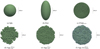 |
Fig. 1 Pilot sample of 1 μm dust grains: 3D representations. All grains are shown using the same scale. All grains are described using dipole sizes of 6.67 nm. |
2.3 Discrete dipole approximation
Multiple options are available to derive the optical constants of dust grains. For instance, Mie theory (Mie 1908) can provide an analytical solution to the scattering of a spherical particle. However, when it comes to spheroids or irregular shapes such as aggregates, numerical methods have to be introduced. In this study, we opted for the use of the discrete dipole approximation (DDA) with the code ADDA (Amsterdam Discrete Dipole Approximation, Yurkin & Hoekstra 2011). The principle of DDA is to discretise entirely the grain into small cubes (‘dipoles’) and give each dipole a complex refractive index.
A restriction that rises with the DDA method is the size of the dipoles. On the one hand, dipoles must be small enough that:
The discretised shape of the grain is geometrically correct and no unwanted surface effects arise.
If we model a mantle, we get a good approximation; a minimum of three dipoles in the mantle thickness is required (Köhler et al. 2015).
The DDA method is valid under the condition |m|kd < 0.5, with d the dipole size, k = 2π/ λ the wave number, and |m| the module of the complex refractive index.
On the other hand, for a given aeff, reducing the size of the dipoles increases the dipole number by a power of 3. The code complexity is linear with the dipole number, so using dipoles too small rapidly becomes computationally prohibitive. Using THEMIS 2.0 with EMT permits one to relax the second constraint, so the main constraint is to ensure the |m|kd < 0.5 criterion.
The grains, in the end, consist of several million dipoles, so huge computational resources are required. Thankfully, ADDA single calculations can be parallelised using MPI2, so we are able to compute efficient and realistic calculations, thanks to the resources of the GENCI at TGCC3.
ADDA computes the interaction of an incoming photon with the dipoles constituting the modelled grain. This calculation can be done at any given wavelength, and thus requires one to perform multiple computations to build the spectral dependency of the grain optical properties. In this study, we carried out calculations for 40 wavelengths, logarithmically distributed from 50 nm to 5 mm. For a better characterisation of the features, the wavelength sampling was refined around 3.1 μm and 200 μm for the ![$\[\text{Agg.:ice}_{1.26 ~\mu \mathrm{m}}^{50 \mathrm{~nm}}\]$](/articles/aa/full_html/2025/06/aa54575-25/aa54575-25-eq8.png) grain, totalling 60 wavelengths for this grain.
grain, totalling 60 wavelengths for this grain.
For non-spherical particles, it is necessary to also take into account the direction of the incoming photon with respect to the grain surface. ADDA allows one to mimic the spatial distribution of the incoming photon direction by rotating the discretised grain along its three Euler angles (α, β, and γ, see Appendix B). For each given orientation, ADDA computes the extinction, Qext, scattering, Qsca, and absorption, Qabs, efficiencies with Qext = Qabs + Qsca. ADDA also computes the Mueller matrix, S (Mueller 1943; Bohren & Huffman 1983), which encapsulates the mathematical description of how light is altered by an optical material describing both intensity (irradiance) and polarisation changes, including a reduction of the total polarisation.
Moreover, not only the direction of the incoming photon must be considered, but also the direction of the scattered photons. Thus, ADDA allows us to compute angle-dependent values of the Mueller matrix, for a range of scattering angles (θ, φ). We note that the first Euler angle, α, is perfectly redundant with the azimuthal scattering angle, φ, so it does not need to be sampled. For the aggregates and the spheroids, we computed, respectively, 24 and 194 combinations of the (β, γ) angles, which permit orientational-averaging.
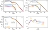 |
Fig. 2 Absorption (a), scattering (b), extinction (c) efficiencies, and emissivity index (d) for the six grains of the pilot sample. We remind the reader that all of the grains have an effective radius of 1 μm for their silicate core and carbon mantle part, while the iced aggregate has a total of aeff = 1.26 μm. Panel d: emissivity index, β, computed as the slope of the extinction efficiency, and shown over a restricted wavelength range, focusing on the sub-millimetre and millimetre. |
3 Results
From the quantities computed with ADDA (Qabs, Qsca, Qext, S), the optical properties of all the grains with the necessary number of dipoles and appropriate orientational-averaging, we derived several different quantities to analyse the emissivity, scattering, and polarisation of the grains. We present these results in this section.
3.1 Emissivity of the modelled dust particles
The emissivity of a dust particle is given by its absorption efficiency, Qabs: it is directly proportional to the absorption cross-section, Cabs, and to the probability of a photon getting absorbed by the grain. In Fig. 2a, we compare the Qabs of the six different 1 μm a-Sil grains described in Sect. 2.2.
The emissivities of all the grains follow the expected common general trend: steady emissivity in the visible at <1 μm, a second regime at infrared wavelengths where the emissivity shows spectral features, and finally a power-law decrease at long wavelengths. At short wavelengths, the different grain models produce achromatic but distinguishable emissivity values, all within an order of magnitude, around 1. Such a difference between grains is expected as the grain structure regulates its absorption capability. In the near- and mid-infrared, the emissivity of all grains shows a structured behaviour. The absorption features in the mid-infrared (MIR) are worth noting: we see the silicate absorption bands at 9.7 and 18 μm and the water absorption bands at 3.1, 12, and 45 μm. In the third regime, in which the wavelength, λ, is large compared to the grain size, aeff, we find that the different grain models produce similar but not identical decreases in emissivity with wavelength. The ‘power-law’ curves do not overlap, but deviate from one grain to another. The slopes of these curves and how they vary will be discussed further in the next section.
3.2 Emissivity index
The emissivity index, β, is the spectral logarithmic slope of the extinction efficiency, Qext, in the far-infrared (FIR) to millimetre range. This also equals the slope of Qabs in the millimetre range, as Qext = Qabs + Qsca and Qsca represents a negligible portion of Qext (< 10−3%) at these wavelengths. We computed the local spectral slope, β(λ), as follows:
![$\[\beta(\lambda)=-\frac{\mathrm{d} log (Q_{\mathrm{ext}})}{\mathrm{d} log (\lambda)}.\]$](/articles/aa/full_html/2025/06/aa54575-25/aa54575-25-eq9.png) (3)
(3)
The wavelength range of interest for β corresponds to the third regime described in Sect. 3.1 (100 μm < λ < 4 mm). In this range, the wavelengths are sampled on 17 points providing 16 β(λ) values, shown in Fig. 2d. For a fixed wavelength value, we observe different values of β from grain to grain, which is influenced not only by the aggregate nature of the grain but also by the substructure of the aggregates themselves. A difference of up to 20% at millimetre wavelengths can be observed, depending only on the bare shape of the grain. The ![$\[\text{Agg.:ice}_{1.26 ~\mu \mathrm{m}}^{50 \mathrm{~nm}}\]$](/articles/aa/full_html/2025/06/aa54575-25/aa54575-25-eq10.png) stands out even more from the non-iced grains. We note that, contrary to a single power law, the spectral indices vary with wavelength. There is structure in the β(λ) curve for all grains, implying slope breaks even at wavelengths longer than 1 mm The emissivity indices range from 1.75 to 2.4 in the millimetre range, and from 2 to 3 in the sub-millimetre range. Even if the β overall stabilises in the millimetre range, we note that it remains wavelength- (or frequency-) dependent. These variations are entirely due to the choice of optical properties for the silicates we use, which come from laboratory measurements down to the millimetre. The optical properties of amorphous solids are known to vary at long wavelengths (see for instance Mennella et al. (1998) for amorphous carbons and Coupeaud et al. (2011) for amorphous silicates). These variations are explained by the disordered structure of amorphous solids on a small scale, as was described in Meny et al. (2007). Previous studies mainly used astrosilicate-type optical properties (Draine & Lee 1984), which were extrapolated to long wavelengths with a constant spectral index, as in the case of crystalline solids. The consequence of this choice was a constant spectral index in the Rayleigh domain (e.g. Draine 2006; Kataoka et al. 2014).
stands out even more from the non-iced grains. We note that, contrary to a single power law, the spectral indices vary with wavelength. There is structure in the β(λ) curve for all grains, implying slope breaks even at wavelengths longer than 1 mm The emissivity indices range from 1.75 to 2.4 in the millimetre range, and from 2 to 3 in the sub-millimetre range. Even if the β overall stabilises in the millimetre range, we note that it remains wavelength- (or frequency-) dependent. These variations are entirely due to the choice of optical properties for the silicates we use, which come from laboratory measurements down to the millimetre. The optical properties of amorphous solids are known to vary at long wavelengths (see for instance Mennella et al. (1998) for amorphous carbons and Coupeaud et al. (2011) for amorphous silicates). These variations are explained by the disordered structure of amorphous solids on a small scale, as was described in Meny et al. (2007). Previous studies mainly used astrosilicate-type optical properties (Draine & Lee 1984), which were extrapolated to long wavelengths with a constant spectral index, as in the case of crystalline solids. The consequence of this choice was a constant spectral index in the Rayleigh domain (e.g. Draine 2006; Kataoka et al. 2014).
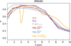 |
Fig. 3 Scattering albedo in the MIR for the six types of silicate grains. All grains have an effective radius of 1 μm for their refractive part (the iced aggregate has a total of aeff = 1.26 μm). |
3.3 Scattering
The integrated scattering efficiencies computed by ADDA, measuring the proportion of scattered light from the total light hitting a grain, are shown in Fig. 2b. The three regimes identified in emissivity can also be distinguished, with large monochromatic scattering efficiencies at wavelengths < 1 μm, large but achromatic values between 1 and 10 μm, and negligible scattering (<10−3) at longer wavelengths.
To examine the spectral dependency of the scattering efficiencies where they show variation (1-10 μm), we computed the scattering albedo of the grains, defined as σ = Qsca/(Qsca + Qabs). This quantity is relative to the total amount of light interacting with the grain, and thus easier to use than Qsca when comparing the relative importance of scattering from grain to grain. Fig. 3 shows that, overall, the scattering albedo of the grains peaks between 0.8 and 0.9 between 1 μm and 6 μm, and then declines towards zero at longer wavelengths. Indeed, at longer wavelengths, the grains are more efficient at absorbing than scattering. The grain coated with ice shows a dip around 3.1 μm, corresponding to absorption in the water band.
The main scattering properties of nonspherical particles are encapsulated in the Mueller matrix elements, S ij (see Mishchenko et al. 2000), which can be used to compute the phase function, ⟨S 11⟩, or the degree of linear polarisation (DLP), −⟨S 12⟩/⟨S 11⟩. The Mueller matrix was computed by ADDA for each scattering angle (θ, φ), and we repeated the computation for each grain orientation (β, γ)5. We averaged S 11 over (β, γ, φ) to infer ⟨S 11(θ)⟩ and show this phase function for the six modelled grains in Fig. 4, plotted at different wavelengths of interest. These wavelengths were chosen as bracketing the size of the grains, aeff, and monomers, a0, as these wavelengths are expected to exhibit the largest scattering efficiencies6.
At first sight, all of the grains show similar phase functions, with no significant departure from the mean trend. As with albedo, the scattering efficiency decreases with wavelength. Furthermore, as wavelength increases, the forth- to back-scattering ratio decreases, as can be seen from the flattening of the phase function (from 106 to 102 at, respectively, λ = 0.05 and 4 μm). We note that the spheres and aggregate with larger monomers scatter more at longer wavelengths, as was expected.
3.4 Polarisation
Starting from the work of Guillet et al. (2018), we defined the normalised direct polarisation induced by a grain (in emission) as Qpol:
![$\[Q_{\mathrm{pol}}=\frac{1}{Q_{\mathrm{abs}}} \frac{Q_{\mathrm{abs}, x}-Q_{\mathrm{abs}, y}}{2}=\frac{Q_{\mathrm{abs}, x}-Q_{\mathrm{abs}, y}}{Q_{\mathrm{abs}, x}+Q_{\mathrm{abs}, y}},\]$](/articles/aa/full_html/2025/06/aa54575-25/aa54575-25-eq11.png) (4)
(4)
Qabs,x and Qabs,y being the absorption efficiencies along the two perpendicular directions of alignment, x and y. The polarisation efficiencies, Qpol, are shown in Fig. 5. For each grain, the absolute polarisation efficiency peaks and then stabilises around 10 μm, while below this threshold Qpol fluctuates, mostly for non-spherical grains, with an amplitude of up to 6 × 10⁻². Overall, we observe significant polarisation only for the Prolate spheroid grain, with absolute values ranging from 10−2 to 0.4 in the FIR and millimetre, while all other grains show values of 10−3 and below in the millimetre range; that is, no significant polarisation.
From the Mueller matrix elements, we measured the scattering polarisation by computing the degree of linear polarisation (DLP, see Bohren & Huffman 1983, p.157):
![$\[P=-\frac{\left\langle S~_{12}\right\rangle}{\left\langle S~_{11}\right\rangle}.\]$](/articles/aa/full_html/2025/06/aa54575-25/aa54575-25-eq12.png) (5)
(5)
In Fig. 6, we plot P against the scattering angle, θ, for a selection of wavelengths from 0.5 to 6 μm. The values are interpolated at the selected wavelengths as in Sect. 3.3.
At long wavelengths, the DLP of all grains tends to behave in the same way, with a bell-shaped curve and a peak in polarisation for a scattering angle of θ = 90°. This corresponds to the Rayleigh scattering (Rayleigh 1871; Bohren & Huffman 1983) that we expect when the wavelengths become large compared to the particle size. At smaller wavelengths, the DLP becomes more erratic for all grains as oscillations appear and differences between grains arise.
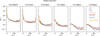 |
Fig. 4 Phase function, ⟨S 11⟩, versus scattering angle. The wavelengths shown were chosen as bracketing the size of the grains, aeff, and monomers, a0, as these wavelengths are expected to exhibit the largest scattering efficiencies. All grains have an effective radius of 1 μm for their refractive part (the iced aggregate has a total of aeff = 1.26 μm). |
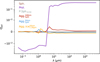 |
Fig. 5 Polarisation efficiency for the six types of grains. The y-axis scale is in sym-log, meaning that the values between −10−2 and 10−2 are plotted on a linear scale to allow the 0 crossing, and the remainder of the axis is on a log scale. |
4 Discussion
The optical properties of the six modelled dust grains, presented in Sect. 3, show significant differences from grain to grain. In this section, we discuss the possible origins of these differences, focusing on the IR and millimetre ranges where most observational studies use the dust emission either to characterize dust properties or indirectly trace other quantities (gas column densities, masses, magnetic fields, etc.).
We emphasise that this study focuses on the optical properties of one grain at a time, and is therefore not strictly comparable with ones that use dust properties obtained from observational probes. For instance, the cross section, ![$\[C_{\text {ext }}=\pi a_{\text {eff }}^{2} Q_{\text {ext }}\]$](/articles/aa/full_html/2025/06/aa54575-25/aa54575-25-eq13.png) , of a single grain of size aeff cannot be compared directly to any line-of-sight integrated quantity, as the latter would result from the combined effects of a population of different grains with a size distribution of n(aeff):
, of a single grain of size aeff cannot be compared directly to any line-of-sight integrated quantity, as the latter would result from the combined effects of a population of different grains with a size distribution of n(aeff):
![$\[\left\langle C_{\mathrm{ext}}(\nu)\right\rangle=\int_{a_{\min }}^{a_{\max }} C_{\mathrm{ext}}\left(a_{\mathrm{eff}}, \nu\right) n\left(a_{\mathrm{eff}}\right) \mathrm{d} a_{\mathrm{eff}} / \int_{a_{\min }}^{a_{\max }} n(a_{\mathrm{eff}}) \mathrm{d} a_{\mathrm{eff}},\]$](/articles/aa/full_html/2025/06/aa54575-25/aa54575-25-eq14.png) (6)
(6)
with no immediate relationship between ⟨Cext⟩ and the single grain properties.
4.1 Validity of approximation for dust structure and porosity in the IR domain
The first thing to note is the difference between the silicate compact grains and the silicate aggregate grains in terms of emissivity at short wavelengths (Fig. 2a). Considering porosity first, all porous silicate grains (aggregates and porous sphere) show an increased emissivity, Qabs, compared to the compact grains in the <1 μm range, with an increase between 90% and 160%. However, in the case of the iced aggregate (yellow curve), the increase in emissivity is moderated. This result illustrates the need to correctly account for grain porosity in the large grain models, which is a natural consequence of random monomer aggregation. Secondly, we can look into detail at the structure of the porous grains. If the porous sphere (grey line) has a similar emissivity, and thus seems a good approximation (<10% difference) for the optical properties of the aggregate (red line) in the <0.5 μm range, its absorption efficiency largely deviates in the near-infrared (NIR). In this latter range, Qabs is lower by a factor of 2 from the aggregate to the porous sphere. We conclude that for wavelengths close to the mean grain size of ~1 μm expected in a dense environment, the modelling of complex aggregates by porous smooth spheres does not allow for a robust interpretation of the data in terms of emission, and hence extinction.
Another key feature at infrared wavelengths is the presence of spectral features or bands. Silicates produce an absorption band at ~10 μm (seen as an increase in Qabs, Fig. 2a) for all silicate grains considered. We stress that the wavelength sampling, which varies slightly between grains, does not allow one to distinguish a band shift between bare grains. However, for ![$\[\text{Agg.:ice}_{1.26 ~\mu \mathrm{m}}^{50 \mathrm{~nm}}\]$](/articles/aa/full_html/2025/06/aa54575-25/aa54575-25-eq15.png) , refined sampling around the water ice features allows one to have greater confidence in the shape and location of these bands. Accounting for the presence of a thin water-ice layer alters the apparent position of the silicate feature, shifting it to large wavelengths as the water-ice 12 μm feature partially merges with the silicate feature. This reinforces the need to consider icy grains when observing dust in dense media in the infrared.
, refined sampling around the water ice features allows one to have greater confidence in the shape and location of these bands. Accounting for the presence of a thin water-ice layer alters the apparent position of the silicate feature, shifting it to large wavelengths as the water-ice 12 μm feature partially merges with the silicate feature. This reinforces the need to consider icy grains when observing dust in dense media in the infrared.
Now looking at the scattering properties, for the albedo (Fig. 3), the interval from 1 to 7 μm is the range where most of the scattering occurs for each grain, with little to no scattering at longer wavelengths. In this range, most of the light goes into scattering, except at 3.1 μm for the ![$\[\text{Agg.:ice}_{1.26 ~\mu \mathrm{m}}^{50 \mathrm{~nm}}\]$](/articles/aa/full_html/2025/06/aa54575-25/aa54575-25-eq17.png) grain due to the strong water-ice feature at this wavelength. On the other hand, the bare grains (without ice mantle) have a similar shape of albedo curve, but we can still note that the
grain due to the strong water-ice feature at this wavelength. On the other hand, the bare grains (without ice mantle) have a similar shape of albedo curve, but we can still note that the ![$\[\operatorname{Agg.}_{1 ~\mu \mathrm{m}}^{100 \mathrm{~nm}}\]$](/articles/aa/full_html/2025/06/aa54575-25/aa54575-25-eq18.png) and
and ![$\[\operatorname{Agg.}_{1 ~\mu \mathrm{m}}^{50 \mathrm{~nm}}\]$](/articles/aa/full_html/2025/06/aa54575-25/aa54575-25-eq19.png) grains have a lower albedo, especially in the 3 to 7 μm range. As with Qabs, the smaller the monomer, the more the properties deviate from those of compact grains. While monomer sizes are related to the equivalent porosity of the aggregate, we note that the effect on Qabs cannot be captured by the porosity effect alone (Ysard et al. 2018). The absolute scattering, Qsca (Fig. 2b), shows the opposite phenomenon, an increase for the aggregates. Hence, the importance of the relative nature of the albedo: the aggregates scatter more than the compact grains in absolute terms at these wavelengths, but they absorb even more, so in proportion their albedo is smaller and depends on the monomer size. As a result, aggregates with small monomers will be observed to scatter less than aggregates with larger monomers, and both these grains will also show lower scattering albedos than the unstructured spheroidal grains. However, the differences in scattering albedo for the grains considered in our sample are small (<20% difference) and probably cannot be probed with the current astronomical instrumentation. Investigating the resulting net scattering albedo of populations of grains on the line of sight is beyond the scope of this paper, but our parametric study of individual grains does not suggest that large variations should be expected due to grain structure.
grains have a lower albedo, especially in the 3 to 7 μm range. As with Qabs, the smaller the monomer, the more the properties deviate from those of compact grains. While monomer sizes are related to the equivalent porosity of the aggregate, we note that the effect on Qabs cannot be captured by the porosity effect alone (Ysard et al. 2018). The absolute scattering, Qsca (Fig. 2b), shows the opposite phenomenon, an increase for the aggregates. Hence, the importance of the relative nature of the albedo: the aggregates scatter more than the compact grains in absolute terms at these wavelengths, but they absorb even more, so in proportion their albedo is smaller and depends on the monomer size. As a result, aggregates with small monomers will be observed to scatter less than aggregates with larger monomers, and both these grains will also show lower scattering albedos than the unstructured spheroidal grains. However, the differences in scattering albedo for the grains considered in our sample are small (<20% difference) and probably cannot be probed with the current astronomical instrumentation. Investigating the resulting net scattering albedo of populations of grains on the line of sight is beyond the scope of this paper, but our parametric study of individual grains does not suggest that large variations should be expected due to grain structure.
The phase function shows the same decrease in scattering with increasing wavelength. In Fig. 4, we see that all grains have a predominant forward-scattering phenomenon with ⟨S 11⟩ several orders of magnitude higher at θ = 0° than at any other scattering angle. At longer wavelengths, when λ becomes similar to and larger than the size of the grains, aeff, the phase function flattens out. The scattering is less intense and becomes close to isotropic. In these ranges, the flattening is more pronounced for the compact grains. All aggregates, ![$\[\text{Agg.}_{1 ~\mu \mathrm{m}}^{100 \mathrm{~nm}}\]$](/articles/aa/full_html/2025/06/aa54575-25/aa54575-25-eq20.png) ,
, ![$\[\text{Agg.}_{1 ~\mu \mathrm{m}}^{50 \mathrm{~nm}}\]$](/articles/aa/full_html/2025/06/aa54575-25/aa54575-25-eq21.png) , and
, and ![$\[\text{Agg.:ice}_{1.26 ~\mu \mathrm{m}}^{50 \mathrm{~nm}}\]$](/articles/aa/full_html/2025/06/aa54575-25/aa54575-25-eq22.png) , together with the P.Sph.0.54 grain, still show at least one order of magnitude between forward- and back-scattering. This implies that in 3D modelling of radiation transfer in a dense environment, depending on the choice of grain structure, heating by near-IR photons will be more pronounced for porous or structured grains in the inner parts. This also has an impact on the prediction of photons scattered outwards. While grain growth mechanisms are not expected to produce spherical compact grains as the main outcome, some specific conditions may lead to compaction of dust grains, especially in disc environments when large dust particles fragment (Michoulier et al. 2024). However, such mechanisms are unlikely to be very efficient for micron-sized grains. Moreover, phase functions from NIR observations probing the ~1 μm dust grains at the surface of discs also suggest that the polarised scattered light comes from Mie scattering of compact grains, favouring particle aggregates as opposed to compact spheres (Engler et al. 2019; Adam et al. 2021). Further modelling of complete dust populations of different sizes and shapes, as well as observational constraints on the polarised emission of dust at different wavelengths are required to lift degeneracies in grain elongation and compactness as they evolve from the diffuse ISM to planet-forming discs.
, together with the P.Sph.0.54 grain, still show at least one order of magnitude between forward- and back-scattering. This implies that in 3D modelling of radiation transfer in a dense environment, depending on the choice of grain structure, heating by near-IR photons will be more pronounced for porous or structured grains in the inner parts. This also has an impact on the prediction of photons scattered outwards. While grain growth mechanisms are not expected to produce spherical compact grains as the main outcome, some specific conditions may lead to compaction of dust grains, especially in disc environments when large dust particles fragment (Michoulier et al. 2024). However, such mechanisms are unlikely to be very efficient for micron-sized grains. Moreover, phase functions from NIR observations probing the ~1 μm dust grains at the surface of discs also suggest that the polarised scattered light comes from Mie scattering of compact grains, favouring particle aggregates as opposed to compact spheres (Engler et al. 2019; Adam et al. 2021). Further modelling of complete dust populations of different sizes and shapes, as well as observational constraints on the polarised emission of dust at different wavelengths are required to lift degeneracies in grain elongation and compactness as they evolve from the diffuse ISM to planet-forming discs.
The degree of linear polarisation is plotted in Fig. 6. Once again, we see a divergence in behaviour between compact and porous grains. As the wavelength becomes large compared to the particle size, as was expected, all grains enter the Rayleigh regime (bell shape): for micron-sized grains, the DLP does not contain any information about grain structure or porosity at λ > 5 μm. However, non-compact grains reach this regime earlier than compact grains: ![$\[\operatorname{Agg.}_{1 ~\mu \mathrm{m}}^{50 \mathrm{~nm}}\]$](/articles/aa/full_html/2025/06/aa54575-25/aa54575-25-eq23.png) already has a Rayleigh-like DLP at 4 μm, and
already has a Rayleigh-like DLP at 4 μm, and ![$\[\operatorname{Agg.}_{1 ~\mu \mathrm{m}}^{100 \mathrm{~nm}}\]$](/articles/aa/full_html/2025/06/aa54575-25/aa54575-25-eq24.png) reaches this behaviour around 4.5 μm, while compact grains do not reach it before 5 μm. Thus, the spectral variation in the DLP can be a good tool to distinguish between grain shapes, should they be compact or aggregated, and could also allow one to distinguish between monomer sizes as well (e.g. Halder et al. 2018; Halder & Ganesh 2021). The P.Sph.0.54 grain follows the trend of
reaches this behaviour around 4.5 μm, while compact grains do not reach it before 5 μm. Thus, the spectral variation in the DLP can be a good tool to distinguish between grain shapes, should they be compact or aggregated, and could also allow one to distinguish between monomer sizes as well (e.g. Halder et al. 2018; Halder & Ganesh 2021). The P.Sph.0.54 grain follows the trend of ![$\[\operatorname{Agg.}_{1 ~\mu \mathrm{m}}^{100 \mathrm{~nm}}\]$](/articles/aa/full_html/2025/06/aa54575-25/aa54575-25-eq25.png) quite well and is therefore a good approximation of the aggregate for the DLP. We note that the
quite well and is therefore a good approximation of the aggregate for the DLP. We note that the ![$\[\text{Agg.:ice}_{1.26 ~\mu \mathrm{m}}^{50 \mathrm{~nm}}\]$](/articles/aa/full_html/2025/06/aa54575-25/aa54575-25-eq26.png) (yellow line) reaches the Rayleigh regime only beyond 6 μm, which is due to its larger effective radius, aeff = 1.26 μm (similar values of the dimensionless coefficient, X = 2πaeff/λ, Tobon Valencia et al. (2024); Tazaki et al. (2021), of about 1.35 are reached at lambda λ = 6 μm for the iced aggregate, while other aggregate grains reach these values around lambda λ = 4.5 μm). We emphasise the sensitivity of the DLP to the grain effective radius, which could be a great tool for grain size measurement. However, this sensitivity could be affected in practice when a whole population of dust sizes is present, rather than the individual grains we consider.
(yellow line) reaches the Rayleigh regime only beyond 6 μm, which is due to its larger effective radius, aeff = 1.26 μm (similar values of the dimensionless coefficient, X = 2πaeff/λ, Tobon Valencia et al. (2024); Tazaki et al. (2021), of about 1.35 are reached at lambda λ = 6 μm for the iced aggregate, while other aggregate grains reach these values around lambda λ = 4.5 μm). We emphasise the sensitivity of the DLP to the grain effective radius, which could be a great tool for grain size measurement. However, this sensitivity could be affected in practice when a whole population of dust sizes is present, rather than the individual grains we consider.
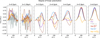 |
Fig. 6 Degree of linear polarisation, |
![$\[-\frac{\left\langle S~_{12}\right\rangle}{\left\langle S~_{11}\right\rangle}\]$](/articles/aa/full_html/2025/06/aa54575-25/aa54575-25-eq16.png)
4.2 Effects of approximating the dust porosity and structure for optical properties in the millimetre domain
With this pilot sample, we are interested in (i) the effect of size on the millimetre emissivity, in other words whether these 1 μm grains have a very different FIR/millimetre β from the 0.1 μm grains for the diffuse medium given in Ysard et al. (2024), and (ii) the effects of porosity and structure on the millimetre emission, in thermal emission and polarisation, in order to discuss whether it is reasonable to approximate these micron-sized grains by spheres when interpreting the data obtained at millimetre wavelengths. Finally, we recall that these grains form the first sample of aggregates from which hypotheses can be constructed to predict the properties of larger aggregates, whose effective sizes will be closer to FIR/millimetre wavelengths.
4.2.1 Optical properties at long wavelengths: Aggregates are different from compact grains
For the compact and porous spherical grains, our models predict spectral indices of β ~ 2.36 at 3 mm. However, our modelled grains made of aggregated monomers show lower β ~ 1.97–2.15 for the ![$\[\text {Agg.}_{1 ~\mu \mathrm{m}}^{50 ~\mathrm{nm}}\]$](/articles/aa/full_html/2025/06/aa54575-25/aa54575-25-eq27.png) and
and ![$\[\text {Agg.}_{1 ~\mu \mathrm{m}}^{100 ~\mathrm{nm}}\]$](/articles/aa/full_html/2025/06/aa54575-25/aa54575-25-eq28.png) , respectively. Our pilot sample thus shows that the spectral index of the dust emissivity at long wavelengths depends on the grain structure: we find significantly lower dust grain emissivities for the aggregated monomer grains than for the compact grains (see Fig. 2). We also note that, in our models of aggregate grains, the smaller the size of the monomer, the lower the emissivity index, given a fixed total volume of material (aeff = 1 μm). Finally, we note that approximating the aggregate structure using porosity alone prevents realistic emissivity indices from being obtained, as the β of the porous sphere remains very close to the compact sphere values and does not mimic that of the aggregate. The physical origins of these long wavelength behaviours are discussed below.
, respectively. Our pilot sample thus shows that the spectral index of the dust emissivity at long wavelengths depends on the grain structure: we find significantly lower dust grain emissivities for the aggregated monomer grains than for the compact grains (see Fig. 2). We also note that, in our models of aggregate grains, the smaller the size of the monomer, the lower the emissivity index, given a fixed total volume of material (aeff = 1 μm). Finally, we note that approximating the aggregate structure using porosity alone prevents realistic emissivity indices from being obtained, as the β of the porous sphere remains very close to the compact sphere values and does not mimic that of the aggregate. The physical origins of these long wavelength behaviours are discussed below.
The reduction in the emissivity index of the aggregates with respect to the compact grains has a subtle cause that lies in the CM structure of the grain material (Ysard et al. 2024) rather than in the purely geometrical modification of the shape. Indeed, all THEMIS 2.0 a-Sil grain models developed for the diffuse medium are coated with a 5 nm mantle of amorphous carbon, irrespective of their size. In the model framework, this mantle results from the accretion of small carbon grains or C atoms from the ISM onto larger silicate seeds, in the diffuse ISM. The relative abundances of carbon and silicate material in the global grain population are maintained by mixing pure carbon grains with these silicate-carbon grains. Starting from a reservoir of the diffuse ISM grains, several scenarios can be considered to describe the evolution of dust in the dense medium towards larger grain sizes.
First, the simplest approach is a scaled-up version of the mechanisms at work in the diffuse ISM. For example, compact growth of a silicate core that retains the spherical geometry of the grain as it grows, then later becomes coated with the smaller carbon grains: this eventually produces large spherical particles of a-Sil, coated with a thin a-C mantle. For a 1 μm spherical grain (such as our compact Sph.), 0.7% of the total mass of the grain is in the form of an a-C mantle for a 5 nm mantle depth.
The second, more realistic scenario, which we explore here, is the aggregation of the small CM monomers from the diffuse ISM, which is enhanced as the gas density increases in the dense medium. In such a scenario, a 1 μm aggregate made up of 100 nm CM monomers, each of which contains 7% of its mass under a-C mantle form, will eventually result in a larger a-C to a-Sil mass ratio than the compact spherical grain of the same size7. Ysard et al. (2018) showed that the millimetre emissivity of the THEMIS a-C material is much flatter than the emissivity of a-Sil materials, for grains made entirely of either one or the other. We can deduce that the flattening of the emissivity of the aggregates compared to the compact shapes is likely due to the increased proportion of a-C material relative to the a-Sil material. We emphasise that the relative mass of the a-C shell increases as aggregates are built from even smaller monomers. This explains the lower emissivity index of the ![$\[\operatorname{Agg.}_{1 ~\mu \mathrm{m}}^{50 \mathrm{~nm}}\]$](/articles/aa/full_html/2025/06/aa54575-25/aa54575-25-eq29.png) grain compared to the
grain compared to the ![$\[\operatorname{Agg.}_{1 ~\mu \mathrm{m}}^{100 \mathrm{~nm}}\]$](/articles/aa/full_html/2025/06/aa54575-25/aa54575-25-eq30.png) grain. Moreover, we find that for a fixed a-C to a-Sil abundance ratio in the grain, both the small grains (0.1 μm representative of the diffuse medium (Ysard et al. 2024, Table 2) and the large aggregate grain
grain. Moreover, we find that for a fixed a-C to a-Sil abundance ratio in the grain, both the small grains (0.1 μm representative of the diffuse medium (Ysard et al. 2024, Table 2) and the large aggregate grain ![$\[\operatorname{Agg.}_{1 ~\mu \mathrm{m}}^{100 \mathrm{~nm}}\]$](/articles/aa/full_html/2025/06/aa54575-25/aa54575-25-eq31.png) have very similar dust emissivity indices β at millimetre wavelengths: a change in grain size of one order of magnitude thus, and unsurprisingly, does not affect the optical properties of the grains when at wavelengths much larger than the grain size. To significantly reduce the β at millimetre wavelengths, one would therefore need to consider a large fraction of dust aggregates of typical sizes >100 μm. The current micron-sized pilot dust grains studied here provide a good elementary brick as monomers of such very large dust particles.
have very similar dust emissivity indices β at millimetre wavelengths: a change in grain size of one order of magnitude thus, and unsurprisingly, does not affect the optical properties of the grains when at wavelengths much larger than the grain size. To significantly reduce the β at millimetre wavelengths, one would therefore need to consider a large fraction of dust aggregates of typical sizes >100 μm. The current micron-sized pilot dust grains studied here provide a good elementary brick as monomers of such very large dust particles.
In summary, the detailed structure of dust grains at the micron scale is not the key to determining their emissivity indices at millimetre wavelengths. However, we stress that the hypothesis made to build up large grains from a population of smaller grains has a significant impact on the expected optical properties at long wavelengths. Indeed, aggregates made of CM monomers inherently have larger mass ratios of a-C to a-Sil, which, in turn, will lead to smaller dust emissivity indices, β, following the a-C material behaviour. Further calculations considering complete dust populations and radiative transfer simulations are needed, but this result is promising in providing an alternative explanation for the low emissivity measured in protostellar environments (Galametz et al. 2019; Cacciapuoti et al. 2023; Bouvier et al. 2021), which can currently only be explained by a large fraction of grains >100 μm (e.g. Ysard et al. 2019), and is at odds with typical timescales from current dust evolution models (Ormel et al. 2009; Silsbee et al. 2022).
In Sect. 3.4, it is noted that the only grain with a significant polarisation efficiency in the far-IR and millimetre range, Qpol > 1%, is the Prol. grain, due to its unique privileged axis, in contrast to the symmetric Sph. and P.Sph.0.54 grains. The aggregates studied, with a high fractal dimension (2.7), are overall spherical, and therefore show only very little (<0.1%) intrinsic polarisation. Although it remains small, this polarisation varies with monomer size: grains with larger monomers are less spherical, and thus polarise light more, as has been shown by Tazaki & Dominik (2022) under disc conditions. We note also that the presence of ice mantles triples the polarisation efficiency, Qpol (see Appendix C). First, we should note that the intrinsic polarisation of a population of prolate grains may not produce any detectable polarised light at far-IR and millimetre wavelengths if the dust particles have no preferred orientation, as the x and y axes would be randomly oriented. The efficiency of polarisation and the efficiency of dust grain alignment are therefore highly degenerate from observational constraints: detailed studies of the alignment physics of complex dust aggregates in magnetised environments, for example, may in the future provide us with a framework that allows us to test predictions from different dust shapes. While theory (Weidenschilling & Cuzzi 1993; Ormel et al. 2007; Dominik 2009) predicts that the first stages of dust growth in the pristine solar nebula create porous fractal aggregates, the prevalence of fractal structures in dust aggregates is also supported by experimental work (Blum & Wurm 2008) and by the detection of fractal aggregates in cometary dust (Mannel et al. 2016). This initial fractal building may later be lost by collisional compaction of the largest dust particles (> mm sizes) in high-density environments, but dust grains evolving in protostellar environments may retain a relatively high fractal dimension, and therefore elongation, although this is still the subject of ongoing research (Tazaki et al. 2023).
4.2.2 Effects of the ice coating
In dense media, protected from the harsh high-energy radiation field at high extinction, low temperatures allow gas to condense on the solid particles. The dust grains are therefore expected to be covered by a mantle of ice, the composition of which will vary according to the local environment. Adding an equal volume of ice to the aggregate grain results in a small difference in effective size, but also marginally modifies the structure of the grain, as the ice is added not only as an outer shell on the aggregate, but also around each monomer. The effects discussed here are a consequence of the properties of water ice rather than these geometrical modifications, as is discussed in Appendix C. In the case of the iced aggregate, we see in Fig. 2 that the millimetre emissivity index is ~10% lower than that of the non-iced counterpart. While such a small difference may not be captured by the current accuracy of observational measurements of the dust emissivity index, the presence of grains covered by layers of ice at specific locations where the temperature drops, within a given object, may result in a flattening of the emissivity. Thus, not only grain growth and complex structures such as the ones naturally formed by aggregation of grains (see Sect. 4.2.1) can explain the overall dust emissivity variations observed in some astrophysical environments. We note that, if ice mantles are responsible for low emissivities at millimetre wavelengths, the spectral feature of silicates at 10 μm should be shifted towards longer wavelengths (see Sect. 4.1).
4.2.3 Effects of silicate composition
Throughout the study, we have used the a-Sil2 material. A relevant addition to the comparisons made in the previous sections is the comparison of the previous grains (a-Sil2) with grains considering a different silicate composition: a-Sil7, which is built with different a forsterite/enstatite abundance ratio and a different enstatite sample, and therefore shows large deviations in its spectral index, β (see Ysard et al. 2024, Table 2). For the sake of simplicity, in this section we limit the study to four grains: Sph., Prol., P.Sph.0.54, and ![$\[\text{Agg.}_{1 ~\mu \mathrm{m}}^{100 \mathrm{~nm}}\]$](/articles/aa/full_html/2025/06/aa54575-25/aa54575-25-eq32.png) grains. For the two silicate compositions considered, we plot the Qabs, Qsca, Qext, and β in Fig. 7. We can see that the emissivity index of the a-Sil7 sphere is significantly lower than that of the sphere made of a-Sil2, meaning that the a-Sil7 silicate material intrinsically has a flatter emissivity in the millimetre range, making it behave more like a-C. The direct consequence of this is that, despite the associated increase in the mass fraction of carbon material, looking at an aggregate dust grain rather than a compact sphere results in a much less dramatic change in the grain emissivity index for the a-Sil7 material than for a grain of a-Sil2. As is explained in Sect. 2.1, we used the EMT approximation, so that the entire a-Sil core/a-C mantle grain structure is encapsulated in one single mock-up material. Figure 8 plots the relative difference,
grains. For the two silicate compositions considered, we plot the Qabs, Qsca, Qext, and β in Fig. 7. We can see that the emissivity index of the a-Sil7 sphere is significantly lower than that of the sphere made of a-Sil2, meaning that the a-Sil7 silicate material intrinsically has a flatter emissivity in the millimetre range, making it behave more like a-C. The direct consequence of this is that, despite the associated increase in the mass fraction of carbon material, looking at an aggregate dust grain rather than a compact sphere results in a much less dramatic change in the grain emissivity index for the a-Sil7 material than for a grain of a-Sil2. As is explained in Sect. 2.1, we used the EMT approximation, so that the entire a-Sil core/a-C mantle grain structure is encapsulated in one single mock-up material. Figure 8 plots the relative difference, ![$\[\epsilon_{k}=\frac{k_{\text {sph.}}-k_{\text {agg.}}}{k_{\text {sph.}}}\]$](/articles/aa/full_html/2025/06/aa54575-25/aa54575-25-eq33.png) , of the imaginary refractive index between the sphere EMT and the aggregate EMT, for the two materials we considered, a-Sil2 and a-Sil7. It shows that since the refractive index of a-Sil7 is already small and close to that of a-C (Ysard et al. 2024), the transition from a sphere to an aggregate adds a-C material but changes only marginally the refractive index for the a-Sil7 aggregate grain, while the effect of adding a-C has much more dramatic consequences on the refractive index of the a-Sil2 aggregate at millimetre wavelengths.
, of the imaginary refractive index between the sphere EMT and the aggregate EMT, for the two materials we considered, a-Sil2 and a-Sil7. It shows that since the refractive index of a-Sil7 is already small and close to that of a-C (Ysard et al. 2024), the transition from a sphere to an aggregate adds a-C material but changes only marginally the refractive index for the a-Sil7 aggregate grain, while the effect of adding a-C has much more dramatic consequences on the refractive index of the a-Sil2 aggregate at millimetre wavelengths.
Regarding the optical properties of dust grains at millimetre wavelengths, changes in composition, structure, and size appear to have significant effects. However, considering grains of sizes up to ~1 μm, such as the ones modelled in this study, does not significantly change the β at millimetre wavelengths. Thus, assuming no larger grains are present, different compositions could be another possible explanation for the diversity of emissivity indices observed among astrophysical objects. Even if the stoichiometry of silicates can change depending on local irradiation conditions (e.g. Demyk et al. 2001), it is not clear how composition of silicates could change within a single dust reservoir that only exhibits small variations in the local physical conditions, such as protostellar envelopes. Other considerations of dust processing mechanisms in specific environments and their consequences for observed dust emissivities should be further investigated.
5 Conclusions
We have studied the optical properties of a pilot sample of six micron-sized dust grains, as analogues of the dust expected to be found in the dense ISM, from the evolution of the small grains shown to be in agreement with diffuse ISM observations (Ysard et al. 2024). Our goal is to evaluate the validity of approximations of the grain structure made when computing the optical properties of complex grains born from the aggregation of small core-mantle grains. With this study, we have focused on exploring the effects of size and grain structure on the resulting optical properties in the IR and millimetre range.
For all six grains, we have investigated emissivity, scattering, and polarisation. The main findings of our study are detailed below.
Up to 20% differences in emissivity indices, in the millimetre, are found, depending on the structure of a grain. Aggregated grains have a significantly lower value of β than their spherical or spheroid equivalent for 1 μm grains.;
When constructing dust grains, and especially aggregates, it is crucial to question the a-C/a-Sil ratio in the constitution of the grain. Particular care must be taken when constructing a dust population to select the correct total relative abundances. Because of the potential differences in the refractive indices of the components, this ratio directly affects the value of the millimetre emissivity index;
The composition of the silicate part of the grain has a significant impact on the emissivity index values. Changing the stoichiometry of silicate mixtures alone changes the β by 25%, as was predicted by the data from Ysard et al. (2024);
The adjunction of water-ice mantles to dust grains, which may be common in the dense ISM, also considerably affects the value of the emissivity index. We found that the spectral indices are almost 10% lower when the grain is covered by an ice mantle, which accounts for half of the total volume;
Lastly, polarisation is highly dependent on the shape of the grains. Asymmetry, and especially a high aspect ratio, induces more polarisation. This means that spheroid grains, oblates or prolates, are good polarisers. Aggregates can also become polarisers when they are fluffy or contain only a few monomers.
These results prove the importance of a good structure representation in the dust models and the need for comprehensive dense medium grains. These grains are the first sample of aggregates from which hypotheses can be made to predict the properties of larger aggregates: a complete grain model, including grains of larger sizes and different structures, will be developed in the future and presented in forthcoming papers. This pilot study will be the basis for performing detailed physical models including dust radiative transfer simulations, and ultimately interpret observations of dust.
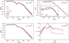 |
Fig. 7 Absorption (a), scattering (b), extinction (c) efficiencies, and emissivity index (d) for four grain structures. The solid lines show the case in which the silicate component is represented by the a-Sil2 material described by Ysard et al. (2024) and the dotted lines the case of the a-Sil7 material. All grains have an effective radius of 1 μm for their refractive part. The emissivity index was computed as the slope of the extinction efficiency, and is zoomed in the sub-mm and millimetre. |
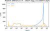 |
Fig. 8 Relative difference between the imaginary part of the refractive index of the Sph. (EMT for a 1000 nm sphere) and of the |
![$\[\text{Agg.}_{1 ~\mu \mathrm{m}}^{100 \mathrm{~nm}}\]$](/articles/aa/full_html/2025/06/aa54575-25/aa54575-25-eq34.png)
Acknowledgements
This project was provided with computing HPC and storage resources by GENCI at TGCC thanks to the grant 2024-A0170415717 on the supercomputer Joliot Curie’s ROME partition. Color sequences in plots of this project are designed to be accessible thanks to Petroff (2021). This work was made possible thanks to the support from the European Research Council (ERC) under the European Union’s Horizon 2020 research and innovation programme (Grant agreement No. 101098309 – PEBBLES).
Appendix A Computing time
As explained in details in Sect. 2.3, the modelling of grains requires a great amount of dipoles in the DDA computations. It means that calculations become really heavy both in terms of required CPU memory and in terms of CPU time. For instance, we need 700 h (CPU) to compute the optical properties of one orientation of the ![$\[\text{Agg.:ice}_{1.26 ~\mu \mathrm{m}}^{50 \mathrm{~nm}}\]$](/articles/aa/full_html/2025/06/aa54575-25/aa54575-25-eq35.png) at 50 nm. All CPU time required for one orientation of the grains for each wavelength are plotted Fig. A.1. This is the reason why we chose to use TGCC resources. Calculations on different orientations and different wavelength are embarrassingly parallel and can be run completely independently with a perfect scaling between the number of CPU and the computing time. However parallelisation of single ADDA computation is a little bit more tricky and requires a little calculation to allocate the right amount of resources.
at 50 nm. All CPU time required for one orientation of the grains for each wavelength are plotted Fig. A.1. This is the reason why we chose to use TGCC resources. Calculations on different orientations and different wavelength are embarrassingly parallel and can be run completely independently with a perfect scaling between the number of CPU and the computing time. However parallelisation of single ADDA computation is a little bit more tricky and requires a little calculation to allocate the right amount of resources.
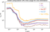 |
Fig. A.1 CPU time of the ADDA computations at each wavelength. Times are given for the computation of 1 orientation and total CPU time would need to be multiplied by 19 for the spheroid and 24 for aggregates. |
From Yurkin & Hoekstra (2011, Eq. (4)), and given the CPU memory on the TGCC machines Mpp = 1.8 Go, we can derive the we can derive the necessary number of processes np for ADDA computation by solving the second order equation:
![$\[\left(-M_{\mathrm{pp}}+384 n_x^2\right) n_{\mathrm{p}}^2+\left(288 n_x^3+271\left(a_{\mathrm{eff}} / d\right)^3\right) n_{\mathrm{p}}+192 n_x^2=0,\]$](/articles/aa/full_html/2025/06/aa54575-25/aa54575-25-eq36.png) (A.1)
(A.1)
where nx represent the size of the computational box in number of dipoles and d is the size of the dipoles. When the number of dipoles gets too high, there is no more real solution to the equation, meaning one must allocate more than 1 CPU to each task to increase the memory per process Mpp. In computations for this study, single computations used between 9 and 32 CPUs at a time.
Appendix B Particle orientation and scattering direction
When computing the optical properties of a dust grain, two sets of angles are of importance. The first angles are referred to as the “orientation of the particle”, and actually determine the position of the incident beam of light relatively to the surface of the grain. These angles are classical “Euler angles” (α, β, γ) representing the orientation of a 3D object in space: α around Oz, then β around the line of nodes and γ around Oz′. The second set of angles determines the outward direction of the light, or scattered beam, and has to be set in reference of the incident beam. Two angles are needed to identify the scattered beam: (θ, φ), φ being the azimuthal angle and dϕ the polar angle. All angles are represented Fig. B.1.
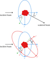 |
Fig. B.1 Representation of the scattering angles (θ, φ) and the Euler angles (α, β, γ). In green is represented the line of nodes (Ox after the first rotation). For comprehension purposes, the incident beam has been set to come from the left of the figure, tilting the figures 90° to the right from the usual spherical coordinates representation (Oz axis pointing upwards). |
Appendix C Comparison of ice addition effect versus same material addition
In this section we give a little more detail on the effects created by the addition of an ice mantle on the dust grains. As noted in the paper, this water ice addition generates an increase in the grain total effective radius. To discriminate between effects due to water ice in itself, and effects due to the modification of the grain’s geometry when adding this mantle, we conducted further study on small (aeff = 100 nm) aggregates.
Three grains were considered: a “standard” grain ![$\[\operatorname{Agg} \cdot{ }_{100 \mathrm{nm}}^{50 \mathrm{nm}}\]$](/articles/aa/full_html/2025/06/aa54575-25/aa54575-25-eq37.png) , constituted of 850 nm monomers, an ice-coated grain
, constituted of 850 nm monomers, an ice-coated grain ![$\[\text { Agg.:ice}_{100 \mathrm{nm}}^{50 \mathrm{nm}}\]$](/articles/aa/full_html/2025/06/aa54575-25/aa54575-25-eq38.png) created identically to
created identically to ![$\[\text {Agg.:} \operatorname{ice}_{1 \mu \mathrm{m}}^{50 \mathrm{nm}}\]$](/articles/aa/full_html/2025/06/aa54575-25/aa54575-25-eq39.png) , and lastly
, and lastly ![$\[\text { Agg.:a-Sil}_{1 \mu \mathrm{m}}^{50 \mathrm{nm}}\]$](/articles/aa/full_html/2025/06/aa54575-25/aa54575-25-eq40.png) , which is essentially the same grain, but instead of the ice mantle, we add a mantle of same EMT material as the bulk grain. The three grains are represented Fig. C.1.
, which is essentially the same grain, but instead of the ice mantle, we add a mantle of same EMT material as the bulk grain. The three grains are represented Fig. C.1.
The results on emissivity index are plotted Fig. C.2 and show, as seen in Sect. 4.2.2, that adding ice mantle to the silicate grains flattens the emissivity. More precisely, we identify here a pure effect of the ice material and no geometric effect: no significant change in the emissivity index is seen in the ![$\[\text { Agg.:a-Sil}_{1 \mu \mathrm{m}}^{50 \mathrm{nm}}\]$](/articles/aa/full_html/2025/06/aa54575-25/aa54575-25-eq41.png) grain compared to
grain compared to ![$\[\text {Agg.}_{100 \mathrm{nm}}^{50 \mathrm{nm}}\]$](/articles/aa/full_html/2025/06/aa54575-25/aa54575-25-eq42.png) . However, we cannot say such for polarisation effects, which are likely due to geometrical effects, as polarisation efficiency differs largely from
. However, we cannot say such for polarisation effects, which are likely due to geometrical effects, as polarisation efficiency differs largely from ![$\[\text {Agg.}_{1 \mu \mathrm{m}}^{50 \mathrm{nm}}\]$](/articles/aa/full_html/2025/06/aa54575-25/aa54575-25-eq43.png) to
to ![$\[\text { Agg.:a-Sil}_{1 \mu \mathrm{m}}^{50 \mathrm{nm}}\]$](/articles/aa/full_html/2025/06/aa54575-25/aa54575-25-eq44.png) .
.
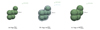 |
Fig. C.1 3D representations of the small aggregates dust grains studied, with dipole size 6.67 nm. All grains are represented with the same scale. |
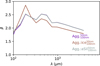 |
Fig. C.2 Emissivity index for the 3 types of silicate grains. The emissivity index is computed as the slope of the extinction efficiency, and is zoomed on the sub-mm and millimetre. |
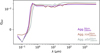 |
Fig. C.3 Polarisation efficiency for the 3 types of grains. The y-axis scale is sym-log, meaning that values between −10−2 and 10−2 are plotted on a linear scale to allow the 0 crossing, and the remaining of the axis is in log scale. |
References
- Adam, C., Olofsson, J., van Holstein, R. G., et al. 2021, A&A, 653, A88 [NASA ADS] [CrossRef] [EDP Sciences] [Google Scholar]
- Birnstiel, T. 2024, ARA&A, 62, 157 [NASA ADS] [CrossRef] [Google Scholar]
- Birnstiel, T., Fang, M., & Johansen, A. 2016, Space Sci. Rev., 205, 41 [Google Scholar]
- Blum, J., & Wurm, G. 2008, ARA&A, 46, 21 [Google Scholar]
- Bohren, C. F., & Huffman, D. R. 1983, Absorption and Scattering of Light by Small Particles (New York, Chichester, Brisbane [Australia]: John Wiley & Sons) [Google Scholar]
- Bouvier, M., López-Sepulcre, A., Ceccarelli, C., et al. 2021, A&A, 653, A117 [CrossRef] [EDP Sciences] [Google Scholar]
- Cacciapuoti, L., Macias, E., Maury, A. J., et al. 2023, A&A, 676, A4 [NASA ADS] [CrossRef] [EDP Sciences] [Google Scholar]
- Compiègne, M., Verstraete, L., Jones, A., et al. 2011, A&A, 525, A103 [Google Scholar]
- Coupeaud, A., Demyk, K., Meny, C., et al. 2011, A&A, 535, A124 [NASA ADS] [CrossRef] [EDP Sciences] [Google Scholar]
- Dartois, E., Noble, J. A., Caselli, P., et al. 2024, Nat. Astron., 8, 359 [NASA ADS] [CrossRef] [Google Scholar]
- Demyk, K., Carrez, Ph., Leroux, H., et al. 2001, A&A, 368, L38 [CrossRef] [EDP Sciences] [Google Scholar]
- Demyk, K., Meny, C., Leroux, H., et al. 2017, A&A, 606, A50 [NASA ADS] [CrossRef] [EDP Sciences] [Google Scholar]
- Demyk, K., Gromov, V., Meny, C., et al. 2022, A&A, 666, A192 [NASA ADS] [CrossRef] [EDP Sciences] [Google Scholar]
- Dominik, C. 2009, in Astronomical Society of the Pacific Conference Series, 414, Cosmic Dust – Near and Far, eds. T. Henning, E. Grün, & J. Steinacker, 494 [Google Scholar]
- Draine, B. T. 2006, ApJ, 636, 1114 [Google Scholar]
- Draine, B. T., & Lee, H. M. 1984, ApJ, 285, 89 [NASA ADS] [CrossRef] [Google Scholar]
- Drążkowska, J., Stammler, S. M., & Birnstiel, T. 2021, A&A, 647, A15 [Google Scholar]
- Dulieu, F., Amiaud, L., Congiu, E., et al. 2010, A&A, 512, A30 [NASA ADS] [CrossRef] [EDP Sciences] [Google Scholar]
- Dullemond, C. P., Juhasz, A., Pohl, A., et al. 2012, Astrophysics Source Code Library [record ascl:1202.015] [Google Scholar]
- Engler, N., Boccaletti, A., Schmid, H. M., et al. 2019, A&A, 622, A192 [NASA ADS] [CrossRef] [EDP Sciences] [Google Scholar]
- Fulle, M., & Blum, J. 2017, MNRAS, 469, S39 [NASA ADS] [CrossRef] [Google Scholar]
- Galametz, M., Maury, A. J., Valdivia, V., et al. 2019, A&A, 632, A5 [NASA ADS] [CrossRef] [EDP Sciences] [Google Scholar]
- Galliano, F., Galametz, M., & Jones, A. P. 2018, ARA&A, 56, 673 [Google Scholar]
- Guillet, V., Fanciullo, L., Verstraete, L., et al. 2018, A&A, 610, A16 [NASA ADS] [CrossRef] [EDP Sciences] [Google Scholar]
- Halder, P., & Ganesh, S. 2021, MNRAS, 501, 1766 [Google Scholar]
- Halder, P., Deb Roy, P., & Das, H. S. 2018, Icarus, 312, 45 [NASA ADS] [CrossRef] [Google Scholar]
- Hensley, B. S., & Draine, B. T. 2023, ApJ, 948, 55 [Google Scholar]
- Herbst, E. 2021, Front. Astron. Space Sci., 8, 207 [NASA ADS] [CrossRef] [Google Scholar]
- Hirashita, H., & Li, Z. Y. 2013, MNRAS, 434, L70 [CrossRef] [Google Scholar]
- Hirashita, H., & Nozawa, T. 2013, Earth Planets Space, 65, 183 [Google Scholar]
- Jäger, A., J., Reissl, Stefan, & Klessen, Ralf S. 2024, A&A, 692, A244 [NASA ADS] [CrossRef] [EDP Sciences] [Google Scholar]
- Jones, A. P. 2011, A&A, 528, A98 [NASA ADS] [CrossRef] [EDP Sciences] [Google Scholar]
- Jones, A. P. 2012a, A&A, 540, A1 [NASA ADS] [CrossRef] [EDP Sciences] [Google Scholar]
- Jones, A. P. 2012b, A&A, 540, A2 [NASA ADS] [CrossRef] [EDP Sciences] [Google Scholar]
- Jones, A. P. 2012c, A&A, 542, A98 [NASA ADS] [CrossRef] [EDP Sciences] [Google Scholar]
- Jones, A. P., Fanciullo, L., Köhler, M., et al. 2013, A&A, 558, A62 [NASA ADS] [CrossRef] [EDP Sciences] [Google Scholar]
- Jones, A. P., Köhler, M., Ysard, N., Bocchio, M., & Verstraete, L. 2017, A&A, 602, A46 [NASA ADS] [CrossRef] [EDP Sciences] [Google Scholar]
- Kataoka, A., Okuzumi, S., Tanaka, H., & Nomura, H. 2014, A&A, 568, A42 [NASA ADS] [CrossRef] [EDP Sciences] [Google Scholar]
- Keppler, M., Benisty, M., Müller, A., et al. 2018, A&A, 617, A44 [NASA ADS] [CrossRef] [EDP Sciences] [Google Scholar]
- Köhler, M., Guillet, V., & Jones, A. 2011, A&A, 528, A96 [NASA ADS] [CrossRef] [EDP Sciences] [Google Scholar]
- Köhler, M., Stepnik, B., Jones, A. P., et al. 2012, A&A, 548, A61 [NASA ADS] [CrossRef] [EDP Sciences] [Google Scholar]
- Köhler, M., Ysard, N., & Jones, A. P. 2015, A&A, 579, A15 [NASA ADS] [CrossRef] [EDP Sciences] [Google Scholar]
- Kozasa, T., Blum, J., & Mukai, T. 1992, A&A, 263, 423 [NASA ADS] [Google Scholar]
- Liu, C., Yin, Y., Hu, F., Jin, H., & Sorensen, C. M. 2015, Aerosol Sci. Technol., 49, 928 [NASA ADS] [CrossRef] [Google Scholar]
- Mannel, T., Bentley, M. S., Schmied, R., et al. 2016, MNRAS, 462, S304 [NASA ADS] [CrossRef] [Google Scholar]
- Mathis, J. S., Rumpl, W., & Nordsieck, K. H. 1977, ApJ, 217, 425 [Google Scholar]
- Maury, A., Hennebelle, P., & Girart, J. M. 2022, Front. Astron. Space Sci., 9, 949223 [NASA ADS] [CrossRef] [Google Scholar]
- Mennella, V., Brucato, J. R., Colangeli, L., et al. 1998, ApJ, 496, 1058 [NASA ADS] [CrossRef] [Google Scholar]
- Meny, C., Gromov, V., Boudet, N., et al. 2007, A&A, 468, 171 [NASA ADS] [CrossRef] [EDP Sciences] [Google Scholar]
- Michoulier, S., Gonzalez, J.-F., & Price, D. J. 2024, A&A, 688, A31 [NASA ADS] [CrossRef] [EDP Sciences] [Google Scholar]
- Mie, G. 1908, Ann. Phys., 330, 377 [Google Scholar]
- Mishchenko, M. I., Hovenier, J. W., & Travis, L. D., eds. 2000, Light Scattering by Nonspherical Particles: Theory, Measurements, and Applications (San Diego: Academic Press) [Google Scholar]
- Mueller, H. 1943, Report of the OSRD project OEMsr-576, 2 [Google Scholar]
- Ormel, C. W., Spaans, M., & Tielens, A. G. G. M. 2007, A&A, 461, 215 [NASA ADS] [CrossRef] [EDP Sciences] [Google Scholar]
- Ormel, C. W., Paszun, D., Dominik, C., & Tielens, A. G. G. M. 2009, A&A, 502, 845 [NASA ADS] [CrossRef] [EDP Sciences] [Google Scholar]
- Ossenkopf, V. 1993, A&A, 280, 617 [NASA ADS] [Google Scholar]
- Ossenkopf, V., & Henning, Th. 1994, A&A, 291, 943 [NASA ADS] [Google Scholar]
- Pagani, L., Steinacker, J., Bacmann, A., Stutz, A., & Henning, T. 2010, Science, 329, 1622 [Google Scholar]
- Petroff, M. A. 2021, arXiv e-prints [arXiv:2107.02270] [Google Scholar]
- Priestley, F. D., De Looze, I., & Barlow, M. J. 2021, MNRAS, 502, 2438 [NASA ADS] [CrossRef] [Google Scholar]
- Rayleigh, L. 1871, Philos. Mag., 41, 107 [Google Scholar]
- Reissl, S., Wolf, S., & Brauer, R. 2016, A&A, 593, A87 [NASA ADS] [CrossRef] [EDP Sciences] [Google Scholar]
- Reissl, S., Nguyen, Philipp, Jordan, Lucas M., & Klessen, Ralf S. 2024, A&A, 692, A60 [NASA ADS] [CrossRef] [EDP Sciences] [Google Scholar]
- Shen, Y., Draine, B. T., & Johnson, E. T. 2008, ApJ, 689, 260 [Google Scholar]
- Siebenmorgen, R. 2023, A&A, 670, A115 [NASA ADS] [CrossRef] [EDP Sciences] [Google Scholar]
- Silsbee, K., Akimkin, V., Ivlev, A. V., et al. 2022, ApJ, 940, 188 [NASA ADS] [CrossRef] [Google Scholar]
- Tazaki, R., & Dominik, C. 2022, A&A, 663, A57 [NASA ADS] [CrossRef] [EDP Sciences] [Google Scholar]
- Tazaki, R., Murakawa, K., Muto, T., Honda, M., & Inoue, A. K. 2021, ApJ, 910, 26 [NASA ADS] [CrossRef] [Google Scholar]
- Tazaki, R., Ginski, C., & Dominik, C. 2023, ApJ, 944, L43 [NASA ADS] [CrossRef] [Google Scholar]
- Teiser, J., Penner, J., Joeris, K., et al. 2025, Nat. Astron., 9, 535 [Google Scholar]
- Testi, L., Birnstiel, T., Ricci, L., et al. 2014, in Protostars and Planets VI, eds. H. Beuther, R. S. Klessen, C. P. Dullemond, & T. Henning, 339 [Google Scholar]
- Tobon Valencia, V., Geffrin, Jean-Michel, Ménard, François, et al. 2024, A&A, 688, A70 [NASA ADS] [CrossRef] [EDP Sciences] [Google Scholar]
- Wakelam, V., Bron, E., Cazaux, S., et al. 2017, Mol. Astrophys., 9, 1 [Google Scholar]
- Warren, S. G. 1984, Appl. Opt., 23, 1206 [NASA ADS] [CrossRef] [Google Scholar]
- Weidenschilling, S. J., & Cuzzi, J. N. 1993, in Protostars and Planets III, eds. E. H. Levy, & J. I. Lunine, 1031 [Google Scholar]
- Weingartner, J. C., & Draine, B. T. 2001, ApJ, 548, 296 [Google Scholar]
- Ysard, N., Jones, A. P., Demyk, K., Boutéraon, T., & Koehler, M. 2018, A&A, 617, A124 [NASA ADS] [CrossRef] [EDP Sciences] [Google Scholar]
- Ysard, N., Koehler, M., Jimenez-Serra, I., Jones, A. P., & Verstraete, L. 2019, A&A, 631, A88 [NASA ADS] [CrossRef] [EDP Sciences] [Google Scholar]
- Ysard, N., Jones, A. P., Guillet, V., et al. 2024, A&A, 684, A34 [NASA ADS] [CrossRef] [EDP Sciences] [Google Scholar]
- Yurkin, M. A., & Hoekstra, A. G. 2011, J. Quant. Spec. Radiat. Transf., 112, 2234 [Google Scholar]
- Zhao, B., Tomida, K., Hennebelle, P., et al. 2020, Space Sci. Rev., 216, 43 [CrossRef] [Google Scholar]
A full description of the model and the associated bibliography are available here: https://www.ias.u-psud.fr/themis/
GENCI stands for “Grand Equipement de Calcul Intensif”, a high-performance computing facility hosted by the TGCC (“Très Grand Centre de Calcul du CEA”), an infrastructure able to host petascale supercomputers: https://www.genci.fr/en
See Fig. B.1 for visualisation of the grain orientation and scattering direction.
All Tables
All Figures
|
Fig. 1 Pilot sample of 1 μm dust grains: 3D representations. All grains are shown using the same scale. All grains are described using dipole sizes of 6.67 nm. |
| In the text | |
|
Fig. 2 Absorption (a), scattering (b), extinction (c) efficiencies, and emissivity index (d) for the six grains of the pilot sample. We remind the reader that all of the grains have an effective radius of 1 μm for their silicate core and carbon mantle part, while the iced aggregate has a total of aeff = 1.26 μm. Panel d: emissivity index, β, computed as the slope of the extinction efficiency, and shown over a restricted wavelength range, focusing on the sub-millimetre and millimetre. |
| In the text | |
|
Fig. 3 Scattering albedo in the MIR for the six types of silicate grains. All grains have an effective radius of 1 μm for their refractive part (the iced aggregate has a total of aeff = 1.26 μm). |
| In the text | |
|
Fig. 4 Phase function, ⟨S 11⟩, versus scattering angle. The wavelengths shown were chosen as bracketing the size of the grains, aeff, and monomers, a0, as these wavelengths are expected to exhibit the largest scattering efficiencies. All grains have an effective radius of 1 μm for their refractive part (the iced aggregate has a total of aeff = 1.26 μm). |
| In the text | |
|
Fig. 5 Polarisation efficiency for the six types of grains. The y-axis scale is in sym-log, meaning that the values between −10−2 and 10−2 are plotted on a linear scale to allow the 0 crossing, and the remainder of the axis is on a log scale. |
| In the text | |
|
Fig. 6 Degree of linear polarisation, |
| In the text | |
|
Fig. 7 Absorption (a), scattering (b), extinction (c) efficiencies, and emissivity index (d) for four grain structures. The solid lines show the case in which the silicate component is represented by the a-Sil2 material described by Ysard et al. (2024) and the dotted lines the case of the a-Sil7 material. All grains have an effective radius of 1 μm for their refractive part. The emissivity index was computed as the slope of the extinction efficiency, and is zoomed in the sub-mm and millimetre. |
| In the text | |
|
Fig. 8 Relative difference between the imaginary part of the refractive index of the Sph. (EMT for a 1000 nm sphere) and of the |
| In the text | |
|
Fig. A.1 CPU time of the ADDA computations at each wavelength. Times are given for the computation of 1 orientation and total CPU time would need to be multiplied by 19 for the spheroid and 24 for aggregates. |
| In the text | |
|
Fig. B.1 Representation of the scattering angles (θ, φ) and the Euler angles (α, β, γ). In green is represented the line of nodes (Ox after the first rotation). For comprehension purposes, the incident beam has been set to come from the left of the figure, tilting the figures 90° to the right from the usual spherical coordinates representation (Oz axis pointing upwards). |
| In the text | |
|
Fig. C.1 3D representations of the small aggregates dust grains studied, with dipole size 6.67 nm. All grains are represented with the same scale. |
| In the text | |
|
Fig. C.2 Emissivity index for the 3 types of silicate grains. The emissivity index is computed as the slope of the extinction efficiency, and is zoomed on the sub-mm and millimetre. |
| In the text | |
|
Fig. C.3 Polarisation efficiency for the 3 types of grains. The y-axis scale is sym-log, meaning that values between −10−2 and 10−2 are plotted on a linear scale to allow the 0 crossing, and the remaining of the axis is in log scale. |
| In the text | |
Current usage metrics show cumulative count of Article Views (full-text article views including HTML views, PDF and ePub downloads, according to the available data) and Abstracts Views on Vision4Press platform.
Data correspond to usage on the plateform after 2015. The current usage metrics is available 48-96 hours after online publication and is updated daily on week days.
Initial download of the metrics may take a while.