| Issue |
A&A
Volume 678, October 2023
|
|
|---|---|---|
| Article Number | A191 | |
| Number of page(s) | 27 | |
| Section | Extragalactic astronomy | |
| DOI | https://doi.org/10.1051/0004-6361/202346113 | |
| Published online | 20 October 2023 | |
GA-NIFS: Black hole and host galaxy properties of two z ≃ 6.8 quasars from the NIRSpec IFU
1
National Research Council of Canada, Herzberg Astronomy & Astrophysics Research Centre, 5071 West Saanich Road, Victoria, BC V9E 2E7, Canada
e-mail: madeline_marshall@outlook.com
2
ARC Centre of Excellence for All Sky Astrophysics in 3 Dimensions (ASTRO 3D), Stromlo, Australia
3
Centro de Astrobiología (CAB), CSIC-INTA, Ctra. de Ajalvir km 4, Torrejón de Ardoz, 28850 Madrid, Spain
4
Kavli Institute for Cosmology, University of Cambridge, Madingley Road, Cambridge CB3 0HA, UK
5
Cavendish Laboratory – Astrophysics Group, University of Cambridge, 19 JJ Thomson Avenue, Cambridge CB3 0HE, UK
6
Department of Physics and Astronomy, University College London, Gower Street, London WC1E 6BT, UK
7
Scuola Normale Superiore, Piazza dei Cavalieri 7, 56126 Pisa, Italy
8
European Space Agency, c/o STScI, 3700 San Martin Drive, Baltimore, MD 21218, USA
9
Department of Physics, University of Oxford, Keble Road, Oxford OX1 3RH, UK
10
Sorbonne Université, CNRS, UMR 7095, Institut d’Astrophysique de Paris, 98 bis Bd Arago, 75014 Paris, France
11
European Space Agency, ESAC, Villanueva de la Cañada, 28692 Madrid, Spain
12
Cosmic Dawn Center (DAWN), Copenhagen, Denmark
13
Niels Bohr Institute, University of Copenhagen, Jagtvej 128, 2200 Copenhagen, Denmark
14
Max Planck Institute for Astronomy, Königstuhl 17, 69117 Heidelberg, Germany
15
INAF – Osservatorio Astrofisco di Arcetri, Largo E. Fermi 5, 50127 Firenze, Italy
16
Centre for Astrophysics Research, Department of Physics, Astronomy and Mathematics, University of Hertfordshire, Hatfield AL10 9AB, UK
17
AURA for the European Space Agency, Space Telescope Science Institute, 3700 San Martin Drive, Baltimore, MD 21218, USA
18
Department of Astrophysical Sciences, Princeton University, 4 Ivy Lane, Princeton, NJ 08544, USA
Received:
7
February
2023
Accepted:
26
August
2023
Aims. Integral field spectroscopy (IFS) with JWST NIRSpec will significantly improve our understanding of the first quasars, by providing spatially resolved, infrared spectroscopic capabilities that cover key rest-frame optical emission lines that have been previously unobservable.
Methods. Here we present our results from the first two z > 6 quasars observed as a part of the Galaxy Assembly with NIRSpec IFS (GA-NIFS) GTO programme, with DELS J0411–0907 at z = 6.82 and VDES J0020–3653 at z = 6.86.
Results. By observing the Hβ, [O III] λλ4959, 5007, and Hα emission lines in these high-z quasars for the first time, we measured accurate black hole masses, MBH = 1.85−0.8+2 × 10⁹ M⊙ and 2.9−1.3+3.5 × 10⁹M⊙, corresponding to Eddington ratios of λEdd = 0.8−0.4+0.7 and 0.4−0.2+0.3 for DELS J0411–0907 and VDES J0020–3653, respectively. These provide a key comparison for existing estimates from the more uncertain Mg II line. We performed quasar–host decomposition using models of the quasars’ broad lines to measure the underlying host galaxies. We also discovered multiple emission line regions surrounding each of the host galaxies, which are likely companion galaxies undergoing mergers with these hosts. We measured the star formation rates, excitation mechanisms, and dynamical masses of the hosts and companions, measuring the MBH/Mdyn ratios at high z using these estimators for the first time. DELS J0411–0907 and VDES J0020–3653 both lie above the local black hole–host mass relation, and are consistent with the existing observations of z ≳ 6 quasar host galaxies with ALMA. We detected ionised outflows in [O III] λλ4959, 5007 and Hβ from both quasars, with mass outflow rates of 58−37+44 and 525−92+75 M⊙ yr−1 for DELS J0411–0907 and VDES J0020–3653, much larger than their host star formation rates of < 33 and < 54 M⊙ yr−1, respectively.
Conclusions. This work highlights the exceptional capabilities of the JWST NIRSpec IFU for observing quasars in the early Universe.
Key words: quasars: supermassive black holes / quasars: emission lines / galaxies: high-redshift / galaxies: interactions / galaxies: active / ISM: jets and outflows
© The Authors 2023
 Open Access article, published by EDP Sciences, under the terms of the Creative Commons Attribution License (https://creativecommons.org/licenses/by/4.0), which permits unrestricted use, distribution, and reproduction in any medium, provided the original work is properly cited.
This article is published in open access under the Subscribe to Open model. Subscribe to A&A to support open access publication.
1. Introduction
Observational surveys over the last two decades have revealed several hundreds of high-z quasars (z ≳ 6; e.g. Fan et al. 2000, 2001, 2003; Willott et al. 2009, 2010; Kashikawa et al. 2015; Bañados et al. 2016, 2018; Banados et al. 2022; Matsuoka et al. 2018; Wang et al. 2019; Yang et al. 2023a), less than a billion years into the Universe’s history. The black holes powering these quasars have been measured to be as massive as ∼1010 M⊙ (Wu et al. 2015), raising questions about the nature of the first black hole seeds and their extreme growth mechanisms. Theories to explain the growth of these first quasars generally require massive black hole seeds, sustained accretion at the Eddington limit, or phases of accretion at super-Eddington rates (e.g. Volonteri & Rees 2005; Volonteri et al. 2015; Sijacki et al. 2009). Some quasars have indeed been measured to have accretion rates above the Eddington limit (e.g. Bañados et al. 2018; Pons et al. 2019; Farina et al. 2022); although, when considering the uncertain black hole mass measurements and a large scatter in the adopted scaling relations, Farina et al. (2022) found no clear evidence for a significant population of super-Eddington high-z quasars. Thus accurate measurements of the black hole mass and accretion rate for high-z quasars provide vital constraints for these theories.
Current high-z quasar black hole mass measurements rely on calibrations that can be quite uncertain. The Hα and Hβ lines are generally considered the most reliable single-epoch indicators of black hole mass, as they are used in many reverberation mapping studies (e.g. Wandel et al. 1999; Kaspi et al. 2000). However, these reverberation mapping studies are performed for low-z, low-luminosity active galactic nuclei (AGN). At higher z, and for luminous quasars, extrapolations are required, and so at high z even these best estimates are uncertain. More critically, for high-z quasars these lines are redshifted into infrared wavelengths > 2.5 μm, beyond the range observable from the ground (for sources at z ≳ 4 for Hβ and z ≳ 3 for Hα). Thus black hole mass measurements for high-z quasars instead have typically relied on the Mg II and C IV lines. Reverberation mapping studies based on Mg II and C IV are more uncertain (e.g. Trevese et al. 2014; Kaspi et al. 2021), and the resulting scaling relations required to obtain single-epoch black hole mass estimates are affected by luminosity-dependent biases and provide highly uncertain mass measurements, for example due to significant blueshifts caused by outflows (e.g. Shen et al. 2008; Shen & Kelly 2012; Peterson 2009; Coatman et al. 2016; Farina et al. 2022, and references within). With the James Webb Space Telescope (JWST; Gardner et al. 2006, 2023; McElwain et al. 2023) and the Near-Infrared Spectrograph (NIRSpec; Jakobsen et al. 2022; Böker et al. 2023), Hβ is now observable up to z = 9.8, and Hα up to z = 7.0 – and beyond with the Mid-Infrared Instrument (MIRI) –, allowing us to more accurately measure the black hole masses and Eddington ratios of high-z quasars with the same estimator at all redshifts (e.g. Eilers et al. 2022; Yang et al. 2023b). This will improve our understanding of the first black holes and their growth rates by determining whether these black holes are truly so massive, and whether they are accreting above the Eddington limit.
Significant questions also exist surrounding the nature of the galaxies in which these quasars reside. These hosts can be measured in the sub-millimetre, tracing their cold gas and dust, which reveals a varying population of objects with a wide range of dynamical masses (1010 − 1011 M⊙), dust masses (107 − 109 M⊙) and sizes (< -pagination1−5 kpc), and star formation rates (SFRs, 10 − 2700 M⊙ yr−1; e.g. Bertoldi et al. 2003; Walter et al. 2003, 2004, 2022; Riechers et al. 2007; Wang et al. 2010, 2011; Venemans et al. 2015, 2017; Willott et al. 2017; Trakhtenbrot et al. 2017; Izumi et al. 2018; Neeleman et al. 2021). However, their host galaxies have not been observed in the rest-frame UV/optical even with the resolution of the Hubble Space Telescope (HST; Mechtley et al. 2012; Decarli et al. 2012; McGreer et al. 2014; Marshall et al. 2020), due to the intense emission from the quasar concealing the small, fainter galaxy underneath (e.g. Schmidt 1963; McLeod & Rieke 1994; Dunlop et al. 2003; Hutchings 2003).
The JWST not only allows us to access the near-infrared spectral range with unprecedented sensitivity, but also provides high angular resolution and a stable point-spread function (PSF). With these improvements over HST, simulations predict that the host galaxies of these high-z quasars will be detectable for the first time (Marshall et al. 2021), and indeed the first signs of host emission have been detected with the Near-Infrared Camera (NIRCam; Ding et al. 2023). Thus JWST and the NIRSpec Integral Field Unit (IFU; Böker et al. 2022) will permit the characterisation of the spatially resolved spectral properties of the hosts, measuring their stellar properties, interstellar medium (ISM) structure and kinematics, excitation mechanisms, and stellar-based SFRs. This will significantly advance our understanding of quasars, their host galaxies, and the rapid growth of early supermassive black holes.
Based on JWST and NIRSpec IFU observations, in this paper we use the standard Hα and Hβ single-epoch black hole mass estimators to derive accurate black hole mass measurements for two z > 6 quasars, DELS J0411–0907 and VDES J0020–3653. DELS J0411–0907 (VHS J0411–0907) at z = 6.82 was discovered independently by Pons et al. (2019) and Wang et al. (2019). DELS J0411–0907 is the most distant of the Pan-STARRS quasars, and is the brightest quasar in the J band above z = 6.7 (Pons et al. 2019). With a relatively low Mg II black hole mass of (6.13 ± 0.51)×108 M⊙, and a bolometric luminosity of (1.89 ± 0.07)×1047 erg s−1, Pons et al. (2019) measured an Eddington ratio of 2.37 ± 0.22, implying that this quasar could be a highly super-Eddington quasar undergoing extreme accretion. The quasar VDES J0020–3653 at z = 6.86 was discovered by Reed et al. (2019). VDES J0020–3653 has a larger Mg II black hole mass than DELS J0411–0907, measured as (16.7 ± 3.2)×108 M⊙ by Reed et al. (2019), and re-derived as 25.1 × 10⁸ M⊙ by Farina et al. (2022) using the Shen et al. (2011) Mg II–black hole mass relation. With a bolometric luminosity of LBol = (1.35 ± 0.03)×1047 erg s−1, these correspond to Eddington ratios of 0.62 ± 0.12 and 0.43, respectively, suggesting that this quasar is powered by a larger supermassive black hole with less extreme accretion than DELS J0411–0907. However, these black hole mass and accretion measurements are based on the Mg II line; robust Hα and Hβ mass estimates will better constrain the accretion of these quasars.
This paper is outlined as follows. In Sect. 2 we describe the JWST NIRSpec observations, and our data reduction and analysis techniques. In Sect. 3 we present our results, with the black hole properties in Sect. 3.1, the host galaxy properties in Sect. 3.2, and the outflow properties in Sect. 3.3. We present a discussion in Sect. 4, before concluding with a summary of our findings in Sect. 5. Throughout this work we adopt the WMAP9 cosmology (Hinshaw et al. 2013) as included in ASTROPY (Astropy Collaboration 2013), with H0 = 69.32 km/(Mpc s), Ωm = 0.2865, and ΩΛ = 0.7134.
2. Data, reduction, and analysis
2.1. Observations
DELS J0411–0907 and VDES J0020–3653 were observed as part of the Galaxy Assembly with NIRSpec Integral Field Spectroscopy (GA-NIFS) Guaranteed Time Observations (GTO) programme, contained within programme #1222 (PI: Willott). This work focuses on the observations of these two quasars with the NIRSpec IFU (Böker et al. 2022), which provides spatially resolved imaging spectroscopy over a 3″ × 3″ field of view with 0.1″ × 0.1″ spatial elements. The IFU observations were taken with a grating/filter pair of G395H/F290LP. This results in a spectral cube with spectral resolution R ∼ 2700 over the wavelength range 2.87−5.27 μm. The observations were taken with a NRSIRS2 readout pattern with 25 groups, using a 6-point medium cycling dither pattern, resulting in a total exposure time of 11 029 s. We constrained the complete position angle (PA) window available for observing these targets with JWST to a more limited PA range, to minimise the leakage of light through the micro-shutter assembly (MSA) from bright sources. Additionally, these quasars have been observed with NIRSpec fixed-slit spectroscopy at shorter wavelengths (with G140H/F070LP, G235H/F170LP), which will be analysed in a separate paper.
DELS J0411–0907 was observed on Oct. 1, 2022, at a PA of 61.893°. VDES J0020–3653 was observed on Oct. 16, 2022, at a PA of 160.169°. Unfortunately, only three out of the six planned dithers were observed due to a spacecraft guiding failure. The final three dithers were observed on Nov. 17, 2022, at a position angle of 188.177°. With half of the VDES J0020–3653 observations observed at a different PA, combining these exposures and their subsequent data analysis was more challenging than the DELS J0411–0907 observations. Due to an error in the reference files of the pipeline (see Perna et al. 2023, for details), we performed a bona fide astrometric registration matching the peak pixel locations of the Hα BLR collapsed images. We applied a constant offset in RA and Dec to the pipeline Stage 1 products of the second set of observations, which allowed the pipeline to correctly combine all six dithers in a final data cube.
Due to an uncertainty in the specified astrometry of our observations, we assumed that the quasar was centred on the known positions from the literature: 04 h 11 m 28.63 s, −09 d 07 m 49.8 s for DELS J0411–0907 (Wang et al. 2019) and 00 h 20 m 31.472 s, −36 d 53 m 41.82 s for VDES J0020–3653 (Reed et al. 2019). These were the targeted positions for our IFU observations, which have been found to have a typical pointing accuracy of ∼0.1″ compared to the requested pointing (Rigby et al. 2022).
2.2. Data reduction
The data reduction was carried out with the JWST calibration pipeline version 1.8.2 (Bushouse et al. 2022), using the context file JWST_1023.PMAP. All of the individual raw images were first processed for detector-level corrections using the DETECTOR1PIPELINE module of the pipeline (Stage 1 hereinafter). The individual products (count-rate images) were then calibrated through CALWEBB_SPEC2 (Stage 2 hereinafter), where WCS-calibration, flat-fielding, and the flux-calibrations are applied to convert the data from units of count rate to flux density. The individual Stage 2 images were then re-sampled and co-added onto a final data cube through the CALWEBB_SPEC3 processing (Stage 3 hereinafter). A number of additional steps and corrections in the pipeline code have been applied to improve the data reduction quality. In particular,
– The individual count-rate frames were further processed at the end of Stage 1, to correct for a different zero-level in the dithered frames. For each image, we therefore subtracted the median value, computed considering the entire image, to get a base-level consistent with zero counts per second.
– We further processed these count-rates to subtract the 1/f noise (Kashino et al. 2022). This correlated vertical noise is modelled in each column (i.e. along the spatial axis) with a low-order polynomial function, after removing all bright pixels (e.g. associated with the observed target) with a sigma-clipping. The modelled 1/f noise was then subtracted before proceeding with the Stage 2 of the pipeline.
– The OUTLIER_DETECTION step of the third and last step of the pipeline is required to identify and flag all remaining cosmic-rays and other artefacts that result in a significant number of spikes in the reduced data. In pipeline version 1.8.2, this step tends to identify too many false positives that compromises the data quality significantly. We therefore implemented a modified version of the LACOSMIC algorithm (van Dokkum 2001) in the JWST pipeline, which was applied at the end of Stage 2 (details in D’Eugenio et al., in prep.).
– We applied the CUBE_BUILD step to produce combined data cubes with a spaxel size of 0.1″, using the exponential modified Shepard method (EMSM) weighting. This provides high signal-to-noise at the spaxel level yet slightly lower spatial resolution with respect to other weightings; the loss in resolution is compensated by the fact that these cubes are less affected by oscillations in the extracted spectra due to re-sampling effects, for example (see Law et al. 2023; Perna et al. 2023, and Appendix C).
We modified the CUBE_BUILD script to fix an error affecting the drizzle algorithm, as implemented in the pipeline version 1.8.5 which was not released at the time of data reduction1. Finally, we also modified the PHOTOM script, applying the corrections implemented in the same unreleased pipeline version2, which allows us to infer more reasonable flux densities (i.e. a factor ∼100 smaller with respect to those obtained with standard pipeline 1.8.2). To test this calibration we also reduced the data using an external flux calibration (details in Perna et al. 2023), and obtained consistent results.
A complete description of the data reduction process and the tests we have performed to ensure its robustness can be found in Perna et al. (2023).
2.3. Data analysis
2.3.1. Quasar and host integrated line fitting
To obtain our integrated quasar spectrum, we integrated our data cube across an aperture of radii 0.35″ for the wavelengths bluewards of the detector gap, and 0.45″ redwards of the gap. These apertures were chosen by examining the PSF structure around Hα and Hβ. These aperture radii contain the central peak of the PSF, but not the ring of reduced flux that occurs prior to the second radial PSF peak. This allowed us to maximise our signal to noise, while containing the majority of the quasar flux.
We compared the flux in this aperture to the total flux in the image (to radius 1.5″) at the peak Hα and Hβ wavelengths, finding an average fraction for both quasars of 81.4% at Hβ, and 86.6% at Hα. We used these percentages as our flux correction, multiplying the integrated aperture flux bluewards of the detector gap by 1.228 and the integrated flux redwards of the detector gap by 1.155.
To fit our quasar spectra we used the Markov chain Monte Carlo (MCMC)-based technique of QUBESPEC3. Our quasar spectra contain Hβ and Hα emission from the BLR, which are blended with the narrow galaxy Hβ, [O III] λλ4959, 5007, and Hα lines (galaxy narrow: ‘GN’), and also with broader lines from the galaxy associated with a kinematically distinct component (e.g. an outflow; galaxy broad: ‘GB’). We note that we saw no evidence for any [N II] λλ6548, 6583 emission in our cubes, from either the quasar or the host galaxies and companions, and so we did not include an [N II] λλ6548, 6583 line in our fit. This likely indicates a low metallicity for our sources.
For the Hα and Hβ lines, we found that the BLR signal cannot be well fit with a single Gaussian. We instead fit the BLR Hα and Hβ lines with a broken power law,
that is convolved with a Gaussian with standard deviation σ (as in e.g. Nagao et al. 2006; Cresci et al. 2015). In our spectral fit we assumed that the galaxy lines were composed of a narrow component (GN), as well as a broad component (GB), which is typically blueshifted and therefore generates a wing in the total profile, which could be attributed to ionised gas outflows. For the two kinematic components, GN and GB, we fit each of the [O III] λλ4959, 5007 and Hβ lines with a Gaussian with velocity offset and line widths equal in velocity space, as each of these lines likely arise from the same physical region with similar kinematics. We tied the amplitude of [O III] λ4959 to be three times less than that of [O III] λ5007, for both GN and GB components. The quasar continuum was modelled as a power law.
The Hα line was fit separately after the [O III] λλ4959, 5007–Hβ complex. The GN Hα component was constrained to have the same velocity as the [O III] λλ4959, 5007 lines. For the Hα GN line width, the Hα GB velocity offset and line width, and the Hα BLR velocity and slopes α1 and α2, the initial guess was the respective Hβ fit property, with normally distributed priors surrounding that value. This is again because the lines likely arise from the same physical region with similar kinematics. We also chose an initial guess for the Hα GN, GB, and BLR peak values to be 3.5 times that of the respective Hβ values, with normally distributed priors around that value, which helps the fit to converge on a Hα model that has realistic flux ratios relative to Hβ. Despite the Hβ–[O III] λλ4959, 5007 and the Hα complexes being fit independently, the agreement among the various kinematic properties was excellent, particularly for the host components (see Table 1). However, for VDES J0020–3653 we note that the Hα BLR full width at half maximum (FWHM) is  km s−1, which is significantly lower than the Hβ FWHM of
  km s−1. This discrepancy may be due to the Hα line being inaccurately measured as it lies close to the edge of the wavelength coverage of the detector; we are more confident in the Hβ line measurement. There are also fit degeneracies which could be affecting this measurement.
Measured line velocity offsets and velocity dispersions (relative to the quoted redshift) from the integrated quasar spectra.
We show the full integrated quasar spectrum for DELS J0411–0907 and VDES J0020–3653 in Fig. 1. In Fig. 2 we show the Hβ and Hα regions of these integrated spectra, alongside the best-fitting model. The velocity offset and FWHM for each of the model components are given in Table 1, and the resulting BLR line fluxes and luminosities are given in Table 2.
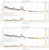 |
Fig. 1. Quasar spectrum for DELS J0411–0907 (top) and VDES J0020–3653 (bottom), showing the spectrum from the brightest spaxel (navy), alongside the integrated spectrum (orange). The integrated spectrum was integrated over a radius of 0.35″ for the wavelengths bluewards of the detector gap, and 0.45″ redwards of the gap, corresponding to the apertures selected for our quasar fitting (Sect. 2.3.1). Our flux corrections of 81.4% and 86.6% have been applied to the integrated spectrum. The spectrum of the brightest spaxel is increased by a constant scaling factor, 8.230 for DELS J0411–0907 and 9.354 for VDES J0020–3653, such that the peak of Hα is equal for both spectra in the plots. The lower panel in each shows the spectra after continuum subtraction. For the brightest spaxel spectrum, the continuum model subtracted from the spectrum is shown in black in the top panel. For the continuum-subtracted integrated spectrum in the lower panel, the integration was performed on the continuum-subtracted cube (i.e. the continuum subtraction was first performed on each of the spaxels individually). The dotted grey vertical lines depict lines of interest at the redshift of the quasar (z = 6.854 for VDES J0020–3653 and z = 6.818 for DELS J0411–0907), and the grey regions show the continuum windows. The detector gap from 4.06 to 4.17 μm has been masked. We note that some minor oscillations are present in the single spaxel spectrum (navy), which can be particularly noticed below 3.3 μm in the single spaxel spectrum. These are caused by spatial undersampling of the PSF, which is a known issue when considering spectra in individual NIRSpec IFU spaxels; we describe this in detail in Perna et al. (2023). When measuring the quasar properties in Sect. 3.1, we used the integrated spectrum (orange), thus removing these single pixel effects. For the quasar subtraction, we found the best performance using the single spaxel spectrum (navy), however these oscillations do not significantly affect our results which directly focus on the regions around Hα and Hβ. |
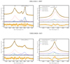 |
Fig. 2. Integrated quasar spectra for DELS J0411–0907 (top) and VDES J0020–3653 (bottom) (orange curve), showing the regions around Hβ (left) and Hα (right). The integrated spectrum was integrated over a radius of 0.35″ for the wavelengths bluewards of the detector gap, and 0.45″ redwards of the gap, corresponding to the apertures selected for our quasar fitting (Sect. 2.3.1). No flux correction has been applied. The best model fit (black) is shown alongside the narrow GN line components (green dot-dashed), the broader GB components (blue dashed lines), and the broken power law component for the BLR (red dotted lines). The lower panels show the residual of the model fit. |
Fluxes and luminosities measured for the 5100 Å continuum, Hα and Hβ BLR lines, alongside the derived black hole masses and Eddington ratios using these properties.
2.3.2. Continuum subtraction
To further analyse our quasar data cubes, we first subtracted the continuum emission from the spectra in each spaxel, by considering the flux in the continuum windows at rest frame 3790–3810 Å, 4210–4230 Å, 5080–5100 Å, 5600–5630 Å and 5970–6000 Å, following Kuraszkiewicz et al. (2002) and Kovacevic et al. (2010); these windows are selected to be uncontaminated by emission lines and blended iron emission. We also added an additional continuum window at the red side of Hα at the edge of the spectral range, at 5.260–5.266 μm in the observed frame, as well as a window near the blue edge of the spectral range, at 2.975–2.990 μm in the observed frame, to better constrain the continuum. We calculated the signal-to-noise ratio (S/N) at each wavelength in each spaxel, taking the noise to be the ‘ERR’ cube produced by the pipeline. For each spaxel in which the median S/N within these continuum windows is greater than 2, we interpolated between these continuum windows using SCIPY’s INTERP1D function using a spline interpolation of second order; this was found to be more robust than fitting a power law curve in each spaxel. In each of these spaxels the interpolation was subtracted from the spectra to create our continuum-subtracted cube. Figure 1 shows the original and continuum-subtracted spectrum of the brightest quasar spaxel.
We note that for VDES J0020–3653 there may be some broad Hα flux in this reddest continuum window in the brightest quasar spaxels, as at this redshift the IFU spectral coverage does not extend to the pure continuum region redwards of Hα. However, we found that this window was necessary for finding a reasonable fit to the continuum around Hα. To reduce any potential effect of this on our results, we used the full, non-continuum subtracted cube in Sect. 2.3.1 when we fit our integrated quasar model to investigate the broad line properties. With our QubeSpec modelling we fit the emission lines as well as the continuum in the form of a power law. As the integrated quasar spectrum is well described by a power law, this approach does not require the continuum window strategy used here. In contrast, within individual spaxels the continuum is not well described by a power law due to the spatial variation of the PSF with wavelength, and so this continuum window approach is more reliable. For our spatially resolved analysis we are primarily interested in the narrow line emission, which is further from the edge of the detector, and so this should be less biased by this issue. However, we do caution that at this high redshift, the Hα measurement of VDES J0020–3653 could be generally susceptible to edge effects from the detector and an imperfect continuum subtraction.
2.3.3. Quasar subtraction
In order to fully understand our quasar–host systems, we decomposed the observed emission into its various components. The aim is to subtract the bright unresolved flux from the quasar, revealing the extended narrow line emission from the host galaxy.
The full cube contains broad line emission from the quasar’s broad-line region (BLR) surrounding the black hole, for example from the Hα and Hβ lines. The BLR is spatially unresolved at these redshifts, and thus this broad line emission is spread spatially according to the PSF of the instrument. In our BLR Quasar Subtraction method (see below), we subtract this BLR component from the cube. The remaining flux in the cube is narrow line emission, for example from [O III] λλ4959, 5007 as well as the Hα and Hβ lines which also have a strong broad component. This narrow emission is emitted both by the quasar’s narrow line region (NLR), photoionised by the AGN and shocks, as well as gas throughout the extended host galaxy (and any companion galaxies) which is photoionised by star formation. While the NLR can be spatially extended, significant NLR emission is produced by the spatially unresolved central region surrounding the AGN, and so this component will clearly trace out the PSF shape. To understand the true spatial extent and kinematics of the extended narrow line emission, and not be biased by the bright unresolved NLR emission, we subtract this narrow unresolved flux from our cube. This is our Narrow & Broad (N&B) Quasar Subtraction, as detailed below.
To separate the host and quasar emission, we used the code QDeblend3D (Husemann et al. 2013, 2014), which uses the relative strength of quasar broad lines in each spaxel to map out the spatial PSF. This strategy allows us to use the specific quasar observation to create an accurate PSF model, instead of relying on an external observation of a known point source (i.e. star) or a theoretical PSF model. The spatial PSF varies with the precise position of the source on the detectors, the general position on the sky, and time, so matching the PSF of our specific observations with a PSF observation or model is less precise than the broad line model we can create here. This methodology has successfully been used for IFU observations of lower-redshift quasar host galaxies (e.g. Husemann et al. 2013, 2014; Vayner et al. 2016; Kakkad et al. 2020).
As the NIRSpec PSF varies with wavelength, we opted to perform the quasar subtraction at two different wavelength regimes. For the spectra bluewards of the detector gap, we used the Hβ line for the subtraction, and for the spectra redwards of the detector gap we used the Hα line for subtraction. This allows for the best subtraction for the wavelength region around each of these two lines.
Step 1, Spatial PSF model. We determined the spatial PSF shape by measuring the relative flux of the quasar BLR at each spatial location. The BLR is spatially unresolved and thus this emission will trace the PSF shape of the instrument. To measure this relative flux we used the continuum-subtracted cube. For Hα, we took the mean of the flux between rest-frame 6500−6523 Å and 6592−6615 Å, either side of the peak of Hα. These broad spectral windows are free from any narrow lines, which would bias the measurement; they are marked in Fig. 3, which shows an example of this quasar subtraction process. For Hβ, the equivalent was performed for emission between rest frame 4800−4830 Å and 4880−4910 Å. Once this broad line flux was measured in each spatial pixel, it was normalised to that of the central brightest quasar spaxel, giving a 2D fractional map of the relative flux of the spatially unresolved BLR, that is, the 2D PSF.
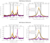 |
Fig. 3. Visualisation of the quasar subtraction using the broad Hβ (left) and Hα (right) lines from DELS J0411–0907. This shows the spectrum in spaxel (23, 24), with the quasar peak located at spaxel (26, 24), in image coordinates. The orange spectrum is the original continuum-subtracted spectrum in the spaxel, containing line flux from both the quasar and host galaxy. The black line is the quasar model spectrum. The top panels show the choice that the quasar model spectrum is that of the central brightest quasar spaxel, which contains both narrow and broad emission – the N&B subtraction. The bottom panel shows the choice that the quasar model spectrum is the BLR component from our best-fit model to the quasar spectrum (Fig. 2) – the BLR subtraction. Using the broad spectral windows marked in grey, the quasar model (black) was scaled to fit the combined spectrum (orange). The purple spectrum shows the residual to that fit, which is the host spectrum. |
To identify spaxels with significant quasar flux from the PSF model, we calculated the S/N in each individual wavelength channel across the selected broad spectral window for each spaxel, using the ‘ERR’ extension as the noise. For our final PSF shape, we selected spaxels in which at least three consecutive wavelength channels had S/N > 10, and then expanded this region spatially by selecting any adjacent spaxels with S/N > 2 over two consecutive wavelength channels, following the FIND_SIGNAL_IN_CUBE algorithm of Sun (2020; see also Sun et al. 2018). To reduce the effect of any artefacts and companion galaxies on the measured PSF shape, we cut the PSF at 10σ, where  and the FWHM is the diffraction limit of the telescope at the observed wavelength of Hβ and Hα, 0.146″ and 0.201″ respectively. This ensures we are only performing the quasar subtraction in regions that have a broad line signal, while ensuring we extract as much of the quasar as possible. The resulting masked PSF shapes are shown in Fig. A.1, for both the Hα and Hβ subtractions for both quasars. Measuring the FWHM of the resulting Hβ PSFs gives 0.18″ for VDES J0020–3653 and 0.16″ for DELS J0411–0907, and 0.23″ for Hα for both VDES J0020–3653 and DELS J0411–0907, consistent with expectations for the PSF size.
Step 2, Quasar spectral model. To perform the quasar subtraction we required a 3D quasar model cube to subtract from the initial quasar and host cube. To create a 3D cube for the quasar emission, alongside the PSF shape (spatial x, y dimensions) we also needed a model for the quasar spectrum (spectral λ dimension), for which we considered two approaches. The first approach was to use the observed spectrum of the brightest spaxel, the centre of the quasar emission, under the assumption that the host line emission is negligible. We refer to this as the ‘N&B Quasar Subtraction’, as this quasar cube includes both the narrow (N) and broad (B) components of the central spectrum, and so both components are subtracted. Our second approach was to use a model of the BLR component of the quasar spectrum. We took this model from our fit to the integrated quasar spectrum (the red curve in Fig. 2, with values quoted in Table 1). This quasar model only includes the BLR component of the fit, and so we refer to this as the ‘BLR Quasar Subtraction’ as only the BLR emission is subtracted from the initial cube. Our process for integrating and fitting the quasar spectrum is described in detail in Sect. 2.3.1.
In our quasar subtraction, the spatial variation of the quasar’s BLR flux was used to determine the PSF shape. However, the N&B subtraction subtracts both the broad and narrow emission that were present in the central quasar spaxel. These emission lines are emitted from the central, unresolved NLR, which is spread according to the PSF shape. This N&B subtraction results in a clear view of the narrow line flux in the underlying, spatially extended host galaxy, without contamination from the bright lines from the central NLR region that have been smeared by the PSF shape. This is ideal for measurements of the spatial distribution and kinematics of emission line regions, as well as measurements of the SFRs which would otherwise be significantly biased by the large amount of AGN-photoionised flux in the centre. However, this method uses the spectrum from the individual brightest quasar spaxel, and so can be subject to observational artefacts that would be removed when integrating over a larger region, for example oscillations in the spectra (see Perna et al. 2023). We chose to use the individual spaxel spectrum and not an integrated spectrum for the model as we found that this resulted in the best quasar subtraction. This model also assumes that the host contribution to the line flux in this central spaxel is negligible, while there may be some small contribution at the position of the optical lines analysed in this work.
In contrast, the BLR quasar subtraction method allows us to view the complete narrow line emission maps, including the contribution of the central unresolved NLR. Our BLR subtraction technique subtracts only the BLR quasar flux, with all of the narrow flux from the central core remaining. Much of this remaining narrow line flux is spread according to the PSF shape, which significantly contaminates any spatial analysis of the extended host region. This approach is also model dependent, varying based on the BLR model fit to the integrated quasar spectrum. With their various advantages and disadvantages, we used both approaches throughout this work.
Step 3, Subtracting the 3D PSF model. For each of these choices for the model quasar spectrum, we scaled the quasar spectrum by the 2D PSF to create a 3D quasar cube. We then subtracted this quasar cube from the original cube, revealing our estimate of the host galaxy’s 3D spectrum. We visually inspected the quasar model fit and residual for a range of spaxels to confirm our subtraction is robust; an example for one spaxel is shown in Fig. 3.
2.3.4. Host line maps
To estimate the noise for our host galaxy maps, we considered that the quasar subtraction introduces additional noise to the resulting host cube that should be accounted for. Following a Monte Carlo process, we generated 200 different realisations of the continuum-subtracted cube with normally distributed noise, where σ was taken from the ‘ERR’ extension from the original cube. We then performed the Hα and Hβ quasar subtraction on each of these 200 cube realisations. To create our modified noise cube, we calculated the standard deviation of these 200 realisations of the quasar subtracted cube at each wavelength in each spaxel.
For the Hβ–[O III] λλ4959, 5007 line complex the values in these noise maps are up to 34% higher than the original noise maps in the central spatial regions of the quasar for the N&B quasar subtraction, and 4% higher for the BLR subtraction. For the Hα line, the values in the noise map are up to 47% higher than the original noise map for the N&B quasar subtraction, and 10% higher for the BLR subtraction. The N&B subtraction introduces more noise than the BLR subtraction, as the N&B quasar model spectrum contains noise while the BLR quasar spectrum is a smooth model and the model uncertainties are not considered in this calculation. The quasar subtraction adds additional uncertainty, particularly where more quasar flux has to be subtracted.
To create maps of the Hα, Hβ, and [O III] λλ4959, 5007 emission of the host galaxy, we fit the spectrum in each spaxel as a series of Gaussians, using ASTROPY’S Levenberg–Marquardt algorithm. We assumed that the narrower galaxy lines are composed of a narrow component (GN) as well as a broader wing (GB; see Sect. 2.3.1). For the GN and GB components, we fit each of the four lines as a Gaussian with mean velocity and line widths equal in velocity space. We tied the amplitude of [O III] λ4959 to be three times less than that of [O III] λ5007, for both the GN and GB components. These theoretical flux ratio constraints provide a good fit for the host galaxy [O III] λλ4959, 5007 lines for both the N&B and BLR quasar subtraction, which gives further confidence in our subtraction techniques. As noted above, we saw no evidence for any [N II] λλ6548, 6583 emission in our cubes, and did not include those lines in our fit.
When the spectrum can be well fit with two Gaussians, the Gaussian with the smallest velocity dispersion σ was assigned as the GN component, while the largest was assigned to the GB component. When only one Gaussian was preferred, if it had σ ≤ 33 Å, or approximately 600 km s−1, it was assigned as a GN component, otherwise as a GB component.
To determine the flux of each of the GN and GB line components we integrated the individual Gaussian model. The S/N was calculated by integrating the noise cube, calculated from the quasar subtraction algorithm, across the same spectral region. Using these noise maps we searched for spaxels with S/N > 5, and then expanded this region spatially by selecting any adjacent spaxels with S/N > 1.5, following the FIND_SIGNAL_IN_CUBE algorithm of Sun (2020). In the maps we only display spaxels meeting this criterion. The resulting maps are shown in Figs. 4 and 6 for the N&B subtraction for DELS J0411–0907 and VDES J0020–3653 respectively, with the BLR subtraction maps for both quasars shown in Fig. B.1 to show the differences between the two subtraction methods.
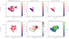 |
Fig. 4. Flux and kinematic maps for DELS J0411–0907, after the subtraction of the quasar emission using the N&B subtraction technique. The top panels show the flux of the narrow component of the [O III] λ5007, Hβ, and Hα lines (GN), as fit by a Gaussian. The bottom left panel shows the flux of the broader GB component of the [O III] λ5007 line, a second Gaussian with a larger σ. The lower middle and right panels show our kinematic maps, showing the non-parametric central velocity of the line (v50; middle) and the line width (w80; right). As these are non-parametric, this combines both the GN and GB components. We describe our method for creating these maps in Sect. 2.3.4. The black ellipses in the lower middle panel depict the regions as in Fig. 5. |
To create velocity maps, we calculated the median velocity v50, a non-parametric measure for the line centre. For the velocity dispersion maps, we calculated w80, the width containing 80% of the line flux. This is a non-parametric measure, which is approximately equal to the FWHM for a Gaussian line (w80 = 1.088 FWHM; see e.g. Zakamska & Greene 2014). The velocity dispersion maps are derived after removing the instrumental width in quadrature at each spaxel, where for NIRSpec in the G395H/F290LP configuration, FWHMinst, Hβ ≃ 115 km s−1, and FWHMinst, Hα ≃ 85 km s−1 for the redshift of these quasars (Jakobsen et al. 2022). These velocity and velocity dispersion maps are also shown in Figs. 4 and 6 for the N&B subtraction, with the BLR subtraction maps also presented in Fig. B.1.
3. Results
3.1. Black hole properties
3.1.1. Redshift
We show the integrated quasar spectrum for DELS J0411–0907 and VDES J0020–3653 in Fig. 2, with the parameters from our spectral fit given in Table 1.
We derived the quasar redshift based on the galaxy narrow (GN) [O III] λ5007 emission. For DELS J0411–0907, we found a redshift of z = 6.818 ± 0.001. This is broadly in agreement with the Lyman-α redshift of DELS J0411–0907, zLyα = 6.81 ± 0.03 (Pons et al. 2019; Wang et al. 2019), and the Mg II redshift, zMg II = 6.824 (Pons et al. 2019).
For VDES J0020–3653, the quasar redshift based on the narrow (GN) [O III] λ5007 emission is z = 6.855 ± 0.002. In comparison, the Lyman-α redshift of VDES J0020–3653 is zLyα = 6.86 ± 0.01 and the Mg II redshift is zMg II = 6.834 ± 0.0004 (Reed et al. 2019). For VDES J0020–3653, there is a significant blueshift of Mg II compared to the [O III] λ5007 and Lyman-α lines.
3.1.2. Black hole masses
Black hole masses can be estimated using the virial relation:
where R is the size of the BLR, ΔV is the width of the emission line, G is the gravitational constant and f is a scale factor. To robustly determine the BLR size R, reverberation mapping studies measure the time delay τ of variability in the emission line to the continuum region, with R = cτ, where c is the speed of light. Empirical correlations have been found between τ and the continuum luminosity of the quasar (e.g. Kaspi et al. 2000), with R ∝ Lγ, allowing the black hole mass to be estimated from single-epoch measurements.
For this work we used the empirically derived relation:
where Greene & Ho (2005) calibrate the constants a and b to be a = (4.4 ± 0.2)×106, b = 0.64 ± 0.02, while alternatively Vestergaard & Peterson (2006) derived a = (8.1 ± 0.4)×106, b = 0.50 ± 0.06. For the quasars under study we measured the continuum-luminosity at rest-frame 5100 Å, L5100 Å, from our integrated quasar spectrum, taking the mean value between 5090–5110 Å to account for noise variations, and using the best-fit redshift of the quasar [O III] λλ4959, 5007 emission (Sect. 3.1.1). Using this and our Hβ broad line FWHM, we calculated the black hole masses using Eq. (3) for both the Greene & Ho (2005) and Vestergaard & Peterson (2006) correlations, which we present in Table 2.
However, the continuum luminosity can be difficult to measure due to contamination by Fe II lines and, for lower luminosity quasars, the host galaxy itself. To circumvent this, Greene & Ho (2005) and Vestergaard & Peterson (2006) derived empirical relations for estimating the black hole mass based solely on the Hβ emission lines:
where Greene & Ho (2005) estimate a = (3.6 ± 0.2)×106, b = 0.56 ± 0.02, while Vestergaard & Peterson (2006) derived a = (4.7 ± 0.3)×106, b = 0.63 ± 0.06. Greene & Ho (2005) also derived a correlation based on the Hα broad line:
Using our measured Hβ and Hα broad line properties, we calculated the black hole masses using Eqs. (4) and (5) for both the Greene & Ho (2005) and Vestergaard & Peterson (2006) correlations. These are also listed in Table 2.
As these empirical black hole mass relations have large scatter, we took the error in these relations to be 0.43 dex, the quoted scatter from Vestergaard & Peterson (2006), and added this in quadrature with our measurement uncertainty from the MCMC fit.
DELS J0411–0907. For DELS J0411–0907, we found that the various scaling relations (Eqs. (3)–(5)) give a black hole mass between 0.9 and 2.5 × 10⁹ M⊙ (Table 2). These measures are all consistent within the uncertainties. We note that while the Hβ−L5100 Å black hole mass estimated by the Greene & Ho (2005) and Vestergaard & Peterson (2006) relations are similar, at 2.0 and 1.7 × 10⁹ M⊙ respectively, the pure Hβ black hole mass estimates are quite different between the two versions of the relation. The Greene & Ho (2005) Hβ relation gives a low black hole mass of 1.3 × 10⁹ M⊙, while the Vestergaard & Peterson (2006) relation gives 2.5 × 10⁹ M⊙, twice as large. This variation between the two scaling relations could be due to the brightness of this quasar, which is brighter than the quasars considered in those studies. We also note that the Greene & Ho (2005) Hα black hole mass for DELS J0411–0907 is 0.9 × 10⁹ M⊙, the lowest of these estimates, yet this is consistent with the other estimates within the uncertainties. As the pure Hβ and Hα relations involve a further calibration from L5100 Å to LHα/Hβ, we opted to take the average of the two MBH,Hβ,5100 Å measurements as our best black hole mass estimate:  . We reiterate that all of these black hole mass estimates are consistent with each other within the uncertainties.
In comparison, from the FWHM of the Mg II line and the rest-frame 3000 Å luminosity measured from Magellan FIRE spectra (Pons et al. 2019), the DELS J0411–0907 black hole mass derived using the Vestergaard & Osmer (2009) relation is MBH,Mg II = (0.61 ± 0.05) × 109 M⊙. This is much lower than our measurements. This quoted error considers only measurement uncertainties, and does not include the additional ∼0.55 dex uncertainty from the scatter in the scaling relation (Vestergaard & Osmer 2009), which would be  . Alternatively, applying the Shen et al. (2011) relation to the same Mg II line FWHM and rest-frame 3000 Å luminosity from Pons et al. (2019), following Farina et al. (2022), we derived MBH,Mg II = 0.95 × 10⁹ M⊙ for DELS J0411–0907. The Mg II line of this quasar was also observed with Keck NIRES, from which the black hole mass was estimated as MBH,Mg II = (0.95 ± 0.09) × 109 M⊙ using the Vestergaard & Osmer (2009) relation (Yang et al. 2021), with an additional ∼0.55 dex uncertainty from the scatter in the scaling relation–
 . While these Mg II black hole masses are all lower than our best estimates, when including the large uncertainty from the scatter in the scaling relations, all of the measurements are consistent.
In summary, the best estimate for the black hole mass of DELS J0411–0907 from NIRSpec IFU,  , is larger than the existing measurements from Mg II, MBH,Mg II = 0.61 − 1 × 10⁹ M⊙. Our measurements used the Hβ–5100 Å black hole mass relation with scatter of ∼0.43 dex, compared with the larger ∼0.55 dex scatter in the Mg II relation, highlighting the benefit of using these Balmer lines as black hole mass estimators.
VDES J0020–3653. For VDES J0020–3653, we found that the various scaling relations give a wide range of black hole mass estimates, between 1.1 and 4.5 × 10⁹ M⊙. These estimates are all consistent within the uncertainties. We note that the lowest measurement is the Hα mass measurement of 1.1 × 10⁹ M⊙. For VDES J0020–3653, the Hα line falls at the edge of the wavelength coverage of the detector, which could cause issues with this measurement. Thus the Hβ measurements of 2.3 − 4.5 × 10⁹ M⊙ are likely more reliable, although all measurements are consistent. As the pure Hβ and Hα relations involve a further calibration from L5100 Å to LHα/Hβ, we opted to take the average of the two MBH,Hβ,5100 Å measurements as our best black hole mass estimate:  . We note again that the Greene & Ho (2005) and Vestergaard & Peterson (2006) black hole masses are quite different, with the Greene & Ho (2005) estimate larger for the Hβ−L5100 Å relation, while the Vestergaard & Peterson (2006) mass is twice as large for the pure Hβ relation. This variation could again be due to the brightness of this quasar, which is brighter than the quasars considered in those studies. We reiterate that all of these black hole mass estimates are consistent within the uncertainties.
In comparison, Reed et al. (2019) measured a black hole mass from the Mg II line and the rest-frame 3000 Å luminosity of MBH,Mg II = (1.67 ± 0.32) × 109 M⊙, using the Vestergaard & Osmer (2009) relation. Accounting for the additional ∼0.55 dex scatter in the Mg II black hole mass relation, this is  . Applying the Shen et al. (2011) relation to the same Mg II line FWHM and rest-frame 3000 Å luminosity from Reed et al. (2019), Farina et al. (2022) derived a larger MBH,Mg II = 2.51 × 10⁹ M⊙. These estimates are in agreement with our estimated black hole mass of
  .
.
For our two quasars, we found that VDES J0020–3653 has a Hβ−L5100 Å black hole mass that is consistent with the existing Mg II black hole mass estimates, while the Hβ−L5100 Å black hole mass for DELS J0411–0907 is larger than the Mg II estimates, albeit consistent within the large uncertainties. Shen et al. (2008) found that for ∼8000 low-z SDSS quasars, log(MBH, Hα/MBH, MgII) follows a Gaussian distribution with mean of 0.034 and dispersion of 0.22 dex, generally indicating a good agreement yet with some quasars found to have significantly different values of log(MBH, Hα/MBH, MgII) up to ±1.5. While high-z quasars may follow a different distribution, our quasars are consistent with this Shen et al. (2008) scenario where Mg II and Hβ mass estimates can be consistent, although for some quasars these estimates can vary significantly. This highlights the need for obtaining Hβ and Hα masses of a larger sample of high-z quasars with JWST, to more accurately measure black hole mass in the early Universe (see also Yang et al. 2023a).
3.1.3. Eddington ratios
We now consider the Eddington Ratio λEdd = LBol/LEdd, the ratio of the quasars’ bolometric to Eddington luminosity.
The quasars’ bolometric luminosities have been estimated from their rest-frame 3000 Å luminosities using the conversion LBol = 5.15 × λL3000 (Shen et al. 2011). Pons et al. (2019) calculated LBol = (1.89 ± 0.07)×1047 erg s−1 for DELS J0411–0907, and Reed et al. (2019) calculated LBol = (1.35 ± 0.03)×1047 erg s−1 for VDES J0020–3653.
The Eddington luminosity, the theoretical maximum luminosity an object could have while balancing radiation pressure and gravity, is typically assumed to be
where G is the gravitational constant, mp the proton mass, c the speed of light, and σT the Thomson scattering cross-section. Using the various black hole mass estimates from Sect. 3.1.2, we calculated the corresponding Eddington ratios which are listed in Table 2.
From our best estimate of the black hole mass for DELS J0411–0907,  , we estimated an Eddington ratio of
  , with our full range of estimates from 0.6−1.6. In comparison, the Pons et al. (2019) estimate of λEdd based on Mg II black hole mass is λEdd,Mg II = 2.37 ± 0.22 for DELS J0411–0907, including only measurement uncertainties and not the scatter in the Mg II black hole mass relation. As discussed in Sect. 3.1.2, instead re-deriving the Mg II black hole mass from the Pons et al. (2019) measurements using the Shen et al. (2011) relation, we calculated λEdd,Mg II = 1.6. With independent spectra, Yang et al. (2021) calculated λEdd,Mg II = 1.3 ± 0.2, again including only measurement uncertainties.
These Mg II-derived ratios are all above the Eddington limit, with the Pons et al. (2019) measurement implying an extremely rapidly accreting quasar. However, our measurements show that the Eddington ratio is  , a more moderate accretion rate. In summary, our results indicate that for DELS J0411–0907 the Mg II measurements underestimate the black hole mass, and thus overestimate the accretion rate of the black hole.
VDES J0020–3653 has a lower bolometric luminosity than DELS J0411–0907, and a larger black hole mass, resulting in a lower Eddington ratio for this quasar. From our best estimate of the black hole mass for VDES J0020–3653,  , we estimated an Eddington ratio of
  , with our full range of estimates from 0.2−0.5, except for the large Hα estimate of
  , which could be affected by its proximity to the edge of the detector. In comparison, the estimate of λEdd based on the Mg II black hole mass was λEdd,Mg II = 0.62 ± 0.12 for VDES J0020–3653 (Reed et al. 2019), or alternatively λEdd,Mg II = 0.43 as re-calculated by Farina et al. (2022). Our derived Eddington ratios are consistent with both values, which all suggest a sub-Eddington accretion rate for this quasar.
3.2. Host galaxy properties
3.2.1. ISM structure and kinematics
In this section we study the spatial structure of the emission line regions present within our data cubes. To verify the spatial structures that we saw, we produced a second set of data cubes by sub-sampling to a pixel scale of 0.05″/pix, and combining the various dithers with a different weighting scheme (see Appendix C), giving higher spatial resolution data cubes. Unfortunately, due to PSF effects the quasar subtraction does not produce successful results using these cubes. As a result, we only used these cubes to qualitatively examine the spatial morphologies in greater detail, with all quantitative results instead using the 0.1″/pix cubes. We show the [O III] λ5007 maps, as measured from these 0.05″/pix data cubes in Fig. C.1, and discuss this further in Appendix C.
DELS J0411–0907. Our quasar-subtracted cube for DELS J0411–0907 reveals three extended narrow-line emission regions, as shown in Fig. 5 and labelled as Regions 1, 2, and 3. These three structures can be seen in both the 0.1″/pix and 0.05″/pix cubes. The integrated spectra for each of the regions are also shown in Fig. 5. Our kinematic maps for the subtracted cube, showing the flux of the lines, their relative velocity, and linewidth in each spaxel are shown in Fig. 4 for the N&B quasar subtraction and in Fig. B.1 for the BLR quasar subtraction. We fit the emission lines in the integrated spectra of each of the three regions with either one or two Gaussians, depending on whether a broader wing component was seen, using the spectral fitting method used to construct our kinematic maps described in Sect. 2.3.4. For Region 2, we excluded the central nine pixels surrounding the quasar peak, as these are highly corrupted by the quasar subtraction and introduce significant noise and artefacts. The extracted flux values and velocities are given in Table 3 and the flux ratios and our derived physical properties are listed in Table 4.
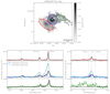 |
Fig. 5. Emission line regions surrounding DELS J0411–0907. Top: the [O III] λ5007 flux map for DELS J0411–0907 after N&B quasar subtraction, with three regions of interest marked. Bottom: the integrated spectrum for the three regions (coloured lines), along with our best fit model in black. The middle panel, for Region 2, also shows the integrated spectra from the BLR quasar subtraction, in cyan, with the best fit model in grey. This region is the host of the quasar (position marked as a cyan cross in the top panel), and so the residual spectrum in this region depends heavily on the type of quasar subtraction. For Regions 1 and 3 the spectrum for both subtraction methods look equivalent, and so the BLR-subtracted spectra are not shown. For Region 2, we exclude the central nine pixels surrounding the quasar peak, as these are highly corrupted by the quasar subtraction and introduce significant noise and artefacts. This means that we slightly underestimate the total flux in this region; however, the fluxes are significantly more reliable than if these nine most corrupted spaxels were included. In Region 1, the spectral lines can be described by a single narrow Gaussian (GN), whereas in Regions 2 and 3 there is also a broader component fit with a second Gaussian (GB); these separate components can be seen as the dashed black lines for the N&B quasar subtraction, and dotted grey lines for the BLR quasar subtraction. |
Flux ratios, SFRs, dust properties, and dust-corrected SFRs for the emission-line regions in DELS J0411–0907 (upper rows) and VDES J0020–3653 (lower rows).
Region 1 is a companion galaxy to the south-east of the quasar. The ellipse defining this region in Fig. 5 is offset 0.78″ from the quasar position. In WMAP9 cosmology at z = 6.818, 1″ = 5.446 kpc, and so this offset is 4.26 kpc, quasar-to-centre. For reference, the region ellipse, which we fit by eye, has a = 0.814″ = 4.4 kpc, b = 0.341″ = 1.9 kpc and a PA of 54.6°. By fitting a 2D Gaussian to the spatial distribution of the [O III] λ5007 flux in this region, we found that this region can be best described with a σa = (0.173 ± 0.007)″ = 0.94 ± 0.04 kpc, an axis ratio of 0.70 ± 0.04, and a PA of 54 ± 4°. We note that this is an unconvolved Gaussian fit to the observed shape, we have not considered the PSF extent or shape to determine an intrinsic size.
From the integrated spectrum, this region has a relative velocity shift of +65 ± 51 km s−1 with respect to the quasar’s peak [O III] λ5007 emission at z = 6.818. The GN Hβ, [O III] λλ4959, 5007, and Hα lines are all detected with a peak S/N > 5, with a line σ of 135 ± 51 km s−1. This region does not contain significant GB flux, with the lines well-fit by a single narrow Gaussian component. Considering instead the cube where only the BLR component of the quasar has been subtracted, the [O III] λλ4959, 5007 properties of Region 1 are relatively unaffected, while the Hβ and Hα fluxes slightly differ; these values are also given in Tables 3 and 4. This region is spatially offset from the quasar such that narrow flux from the central spaxel, smeared by the PSF, does not contribute strongly. However, some quasar flux is present, hence the slightly different results for the different quasar subtractions.
Region 2 is the host galaxy of the quasar. The circle defining this region in Fig. 5 has a radius r = 0.458″ or 2.5 kpc, for reference. By fitting a 2D Gaussian to the spatial distribution of the [O III] λ5007 flux in this region, we found that this can be best described with a σa = 0.14 ± 0.02″ = 0.75 ± 0.09 kpc, an axis ratio of 0.81 ± 0.14, and a PA of 83 ± 20°. The GN Hβ, [O III] λλ4959, 5007, and Hα lines are detected with a S/N ≥ 17, while the brighter [O III] λλ4959, 5007 lines also exhibit a broader (GB) wing, detected with S/N ≥ 9. The GN line is offset from the quasar at z = 6.818 by +163 ± 51 km s−1, with a line σ of 314 ± 51 km s−1, while the broader wing is offset by −783 ± 51 km s−1 with a line σ of 526 ± 51 km s−1.
These line properties for Region 2 vary significantly when considering the BLR quasar subtracted cube, that has removed only the BLR model of the quasar, instead of the N&B quasar subtracted cube, in which unresolved NLR flux from the centre of the galaxy is also removed. The line properties for the BLR subtracted cube are presented in Table 3, alongside the N&B subtracted properties. The integrated spectrum of this region is also shown for the BLR-subtracted cube in Fig. 5, and clearly contains significantly more flux than for the N&B quasar subtracted cube. This central region is coincident with the quasar, and so this BLR subtracted cube contains the unresolved narrow line flux from the NLR surrounding the quasar, spread across the image according to the PSF shape. This can also be seen in the flux maps for this BLR-subtracted cube, presented in Fig. B.1, which show the bright central narrow line emission. In the BLR-subtracted cube there is significant GB flux, offset by −374 ± 51 km s−1 from the quasar’s GN [O III] λ5007 peak, with a line σ of 807 ± 51 km s−1.
Region 3 sits to the north-west of the quasar. The ellipse we fit by eye to define this region in Fig. 5 is offset 0.90″ = 4.9 kpc from the quasar centre-to-centre, with a = 0.509″ = 2.8 kpc, b = 0.235″ = 1.3 kpc and a PA of 72.1°. This region is not well fit by a 2D Gaussian, so we did not constrain its σ and axis ratio as for the other regions. From the integrated spectrum of this region there are significant detections of [O III] λλ4959, 5007 GN components and a broader [O III] λ5007 GB component, with a marginal detection of an [O III] λ4959 GB component. No Hα or Hβ is significantly detected. The GN line component is offset from the quasar at z = 6.818 by +396 ± 51 km s−1, with a line σ of 161 ± 51 km s−1, while the broader GB wing is offset by +38 ± 51 km s−1 with a line σ of 764 ± 51 km s−1. With its larger relative velocity and line width, and non-Gaussian spatial distribution, Region 3 is likely a tidal tail. As for Region 1, the BLR subtracted cube produces consistent results to the N&B quasar-subtracted cube in this region, as Region 3 is spatially offset enough that the narrow-line flux from the quasar has negligible contribution.
VDES J0020–3653. Our quasar-subtracted cube for VDES J0020–3653 also reveals three extended narrow-line emission regions, with their [O III] λ5007 flux and integrated spectra shown in Fig. 7. The [O III] λ5007 maps made using the higher spatial resolution 0.05″/pix cubes (Fig. C.1) expose a fourth emission line region, separated by only ∼0.37″ or 2 kpc (quasar peak to companion peak) to the south-south-west of the quasar. This is so close to the quasar host that in the 0.1″/pix cubes this appears to be one elongated host galaxy. Using the spatial structure from the higher resolution cube, we defined four region ellipses from which we extracted the spectra in each region. Thus, while the 0.1″/pix cubes can barely distinguish the host and this nearby companion galaxy, using the additional spatial information from the higher resolution cubes we were able to more accurately measure the host galaxy properties from the 0.1″/pix cubes, excluding the additional flux from the nearby companion. The extracted flux values from each of the four region ellipses are given in Table 3, with their flux ratios and derived physical properties in Table 4. Our kinematic maps for the subtracted cube, showing the flux of the lines, their relative velocity, and linewidth in each spaxel are shown in Fig. 6 for the N&B quasar subtraction and Fig. B.1 for the BLR quasar subtraction.
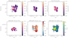 |
Fig. 6. Kinematic maps for VDES J0020–3653, after the subtraction of the quasar emission using the N&B subtraction technique. The top panels show the flux of the narrow component of the [O III] λ5007, Hβ, and Hα lines (GN), as fit by a Gaussian. The bottom left panel shows the flux of the broader GB component of the [O III] λ5007 line, a second Gaussian with a larger σ. The lower middle and right panels show our kinematic maps, showing the non-parametric central velocity of the line (v50; middle) and the line width (w80; right). As these are non-parametric, this combines both the GN and GB components. We describe our method for creating these maps in Sect. 2.3.4. The black ellipses in the lower middle panel depict the regions as in Fig. 7. |
Region 1 is a companion galaxy to the south-south-west of the quasar, with such a small separation that it is barely resolvable in the 0.1″/pix cube. The ellipse defining this region in Fig. 7 is offset 0.52″ from the quasar position. In WMAP9 cosmology at z = 6.854, 1″ = 5.429 kpc, and so this offset is 2.8 kpc, quasar-to-centre. The ellipse has a = 0.338″ = 1.8 kpc, b = 0.228″ = 1.2 kpc and a PA of 109°. As this region is blended with the host emission at this small separation, the emission does not follow a 2D Gaussian profile and so we did not quote the best fitting parameters as for the other regions. From the integrated spectrum, this region has a relative velocity shift of −30 ± 51 km s−1 with respect to the quasar’s peak [O III] λ5007 emission at z = 6.854. The GN Hβ, [O III] λλ4959, 5007, and Hα lines are all detected with a S/N ≥ 11, with a line σ of 319 ± 51 km s−1. These lines are well-fit by a single Gaussian component, with no secondary GB flux detected. When using the BLR subtracted cube, the flux is measured to be slightly larger due to contamination by the narrow-line flux from the quasar at this separation. The flux seen around [N II] λ6583 in Region 1 is likely remaining broad Hα flux from the quasar.
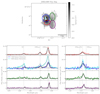 |
Fig. 7. Emission line regions surrounding VDES J0020–3653. Top: the [O III] λ5007 flux map for VDES J0020–3653 after N&B quasar subtraction, with four regions of interest marked. Bottom: the integrated spectrum for the four regions (coloured lines), along with our best fit model in black. The middle panel, for Region 2, also shows the integrated spectra from the BLR quasar subtraction, in cyan, with the best fit model in grey. This region is the host of the quasar (position marked as a cyan cross in the top panel), and so the residual spectrum in this region depends heavily on the type of quasar subtraction. We note that to account for the overlapping area between Regions 1 and 2, we assigned the flux in those spaxels to Region 1 only. For Region 2, we excluded the central nine pixels surrounding the quasar peak, as these are highly corrupted by the quasar subtraction and introduce significant noise and artefacts. This means that we slightly underestimate the total flux in this region, however the fluxes are significantly more reliable than if these nine most corrupted spaxels were included. In Regions 1, 3, and 4, the spectral lines can be described by a single narrow Gaussian (GN), whereas in Region 2 there is also a broader component which we fit with a second Gaussian (GB); these separate components can be seen as the dashed black lines for the N&B quasar subtraction, and dotted grey lines for the BLR quasar subtraction. We note that the emission around 3.8 μm in Regions 3 and 4 is likely an artefact in the cube. We did not see any significant detection of [N II] λλ6548, 6583. |
Region 2 is the host galaxy of the quasar. For reference, the circle defining this region in Fig. 7 has a radius r = 0.385″ = 2.1 kpc. By fitting a 2D Gaussian to the spatial distribution of the [O III] λ5007 flux in this region, we found that this can be best described with a σa = (0.18 ± 0.02)″ = (1.0 ± 0.1) kpc, an axis ratio of 0.66 ± 0.12, and a PA of 26 ± 10°. The GN [O III] λλ4959, 5007, Hβ and Hα lines are detected with a S/N ≥ 2.6. The brighter [O III] λλ4959, 5007 lines also exhibit a broader (GB) wing, detected with S/N ≥ 1.4. The GN line is offset from the quasar at z = 6.854 by +149 ± 51 km s−1, with a line σ of 369 ± 51 km s−1, while the broader wing is offset by −877 ± 51 km s−1 with a large line σ of 698 ± 51 km s−1.
As for the host region in DELS J0411–0907, the VDES J0020–3653 line properties for Region 2 vary significantly when considering the BLR quasar subtracted cube. The line properties for the BLR subtracted cube are presented in Table 3, alongside the N&B subtracted properties, and the integrated spectrum for Region 2 for the BLR subtraction is also shown in Fig. 7. As for DELS J0411–0907, this central region is coincident with the quasar, and so this BLR subtracted cube contains the unresolved narrow line flux from the NLR surrounding the quasar, spread across the image according to the PSF shape. This can also be seen in the kinematic maps for this cube, presented in Figs. 6 and B.1, which show the bright central emission.
Region 3 is likely a second companion galaxy to the north-west of the quasar. The ellipse defining this region in Fig. 7 is offset 0.77″ = 4.17 kpc from the quasar centre-to-centre, with a = 0.417″ = 2.3 kpc, b = 0.271″ = 1.5 kpc and a PA of 11°. By fitting a 2D Gaussian to the spatial distribution of the [O III] λ5007 flux in this region, we found that this can be best described with a σa = (0.4 ± 0.1)″ = (2.0 ± 0.5) kpc, an axis ratio of 0.6 ± 0.2, and a PA of 193 ± 5°. In this region there are significant detections of GN [O III] λλ4959, 5007, Hβ and Hα components, with S/N ≥ 8.9. The GN line component is offset from the quasar at z = 6.854 by +232 ± 51 km s−1, with a line σ of 250 ± 51 km s−1. No broader GB component is detected. The properties of Region 3 are relatively unaffected when considering instead the BLR quasar subtracted cube; these are also given in Tables 3 and 4. This region is spatially offset from the quasar such that no significant narrow flux from the central region contributes.
Region 4 is a companion galaxy to the south-west of the quasar. The ellipse defining this region in Fig. 7 is offset 1.03″ = 5.61 kpc from the quasar position, quasar-to-centre. For reference, the region ellipse that we fit by eye has a = 0.439″ = 2.4 kpc, b = 0.299″ = 1.6 kpc and a PA of 0°. By fitting a 2D Gaussian to the spatial distribution of the [O III] λ5007 flux in this region, we found that this region can be best described with a σa = 0.43 ± 0.08″ = 2.3 ± 0.4 kpc, an axis ratio of 0.47 ± 0.13, and a PA of −4 ± 2°. We note again that this is an unconvolved Gaussian fit to the observed shape. From the integrated spectrum, this region has a relative velocity shift of +367 ± 51 km s−1 with respect to the quasar’s peak [O III] λ5007 emission at z = 6.854. The GN Hβ, [O III] λλ4959, 5007, and Hα lines are all detected with a S/N ≥ 13, with a line σ of 189 ± 51 km s−1. These lines are well-fit by a single Gaussian component, with no GB flux detected. As for Region 3, the BLR subtracted cube has consistent results to the N&B quasar-subtracted cube, as Region 4 is spatially offset enough that the narrow-line flux from the quasar has negligible contribution.
3.2.2. Limits on star formation rates and excitation mechanisms
Using our integrated spectrum for each region, we estimated the SFR using the GN Hα line flux. Assuming no extinction, a solar abundance, and a Salpeter IMF, the SFR can be estimated as:
(Kennicutt & Evans 2012, we note that these values are 68% of those calculated assuming the Kennicutt 1998 relation). We used this equation to calculate the SFR for each of the regions in which Hα is detected. The resulting SFRs for DELS J0411–0907 and VDES J0020–3653 are given in Table 4.
This equation assumes that all of the Hα emission is from star formation; for our host galaxies, however, we note that even for our N&B quasar subtracted cubes we expect some AGN-photoionised narrow line flux to contribute. The N&B quasar subtraction removes all of the GN component that is emitted from the central unresolved region surrounding the quasar, although spatially resolved GN flux from both the NLR and star formation remains. Thus, while the N&B quasar subtracted cubes provide the most accurate measurement of the SFRs of our emission-line regions, in comparison to the BLR subtracted cubes, for our host components these are upper limits. For comparison, we also include the SFRs calculated using the BLR quasar subtracted cube in Table 4, which includes all quasar NLR emission, showing the significant improvement that the narrow-line quasar subtraction can have on being able to measure host galaxy properties. For DELS J0411–0907, the host SFR measured from the N&B subtraction is < 33 M⊙ yr−1, whereas the BLR subtraction can only constrain the SFR to < 91 M⊙ yr−1, a much larger upper limit. The host galaxy of VDES J0020–3653 has SFR constraints of < 55 M⊙ yr−1, consistent for both the BLR and N&B subtractions, likely due to the noisy subtraction around Hα.
In the absence of dust extinction, theoretically the ratio of Hα to Hβ flux is FHα/FHβ ≃ 2.86, estimated using a temperature T = 104 K and an electron density ne = 102 cm−3 for Case B recombination (Osterbrock 1989; Domínguez et al. 2013). Hence, the amount of dust can be estimated from these two lines via E(B − V) = 1.97log10[(FHα/FHβ)/2.86] following Domínguez et al. (2013), and so AHα = (3.33 ± 0.80)×E(B − V) assuming the Calzetti et al. (2000) reddening law. For companion regions where both Hα and Hβ are significantly detected and FHα/FHβ > 2.86, we calculated E(B − V), AHα and a dust-corrected SFR, which are given in Table 4. As the host regions contain NLR quasar-photoionised flux which can have significantly higher Hα/Hβ ratios than the 2.86 assumed here, we did not calculate dust-corrected SFR limits for the host galaxies.
For DELS J0411–0907, the companion galaxy Region 1 has a SFR of 27 ± 1 M⊙ yr−1, as measured from the N&B quasar subtracted spectrum. As the FHα/FHβ ratio is < 2.86, we did not estimate the dust corrected values. These flux ratios are unlikely to be truly < 2.86, with this more likely being an issue with the quasar subtraction technique and its removal of flux, as the N&B subtraction has FHα/FHβ = 2.4 ± 0.1 while the BLR subtraction has FHα/FHβ = 2.8 ± 0.1. The BLR quasar subtraction results in slightly more Hα flux, corresponding to a SFR of 29 ± 1 M⊙ yr−1, as well as a lower Hβ flux which also contributes to the larger FHα/FHβ. For this region only, we therefore consider the BLR subtraction to provide the best estimate of the SFR, 29 ± 1 M⊙ yr−1, whereas for all other regions the N&B subtraction provides the best estimate.
For VDES J0020–3653, the companion galaxy Region 1 has a SFR of 24 ± 2 M⊙ yr−1 as measured from the N&B quasar subtracted spectrum, or 51 yr−1 when corrected for dust attenuation. Using the BLR subtraction, the SFR is similarly 26 ± 2 M⊙ yr−1. However, this subtraction results in a much lower Hα/Hβ ratio of 2.91 ± 0.3, due to contamination from the unresolved quasar emission, and so in this case there is minimal change in the SFR when corrected for dust attenuation, 27
 yr−1. The companion galaxy Region 3 has a SFR of 18 ± 2 M⊙ yr−1, as measured from the N&B quasar subtracted spectrum, or 70
 yr−1 when corrected for dust attenuation, due to its large Hα/Hβ ratio. Region 4 has a SFR of 17 ± 1 M⊙ yr−1, as measured from both the N&B quasar subtracted and BLR quasar subtracted spectrum. When corrected for dust-attenuation, this SFR increases to 42
 yr−1. The subtraction method makes little difference for the companion regions 3 and 4, which are sufficiently spatially separated from the quasar such that the unresolved quasar emission has little contribution (see Table 4).
We note that our quasar hosts and companion galaxies have no detected [N II] λλ6548, 6583 emission, implying low metallicities. For our SFR calculation we used the typically used conversion from Hα in Eq. (7), which is calculated for solar abundances. Lee et al. (2009) recalculated the SFR–LHα relation for a range of metallicities using the Bruzual & Charlot (2003) population synthesis models. Assuming a case B recombination with nebular temperature of 104 K, a density of 100 cm−3, and a Salpeter IMF, Lee et al. (2009) found that the ratio SFR/LHα in Eq. (7) decreases from 7.9 × 10−42 at Z = Z⊙, to 6.2 × 10−42 at Z = 0.2 Z⊙ and 5.2 × 10−42 at Z = 0.02 Z⊙. This would reduce our calculated SFRs by 22% and 34%, respectively.
We did not detect any [N II] λλ6548, 6583 emission from our quasars, their hosts or their companions. To place upper limits on the amount of [N II] λ6583 present in the different emission-line regions, we integrated the ERR array at the expected location of the line, assuming a line width equal to that of [O III] λ5007. Our [N II] λ6583 limits are given in Table 3, with the resulting [N II] λ6583/Hα flux ratio limits in Table 4.
Using our measured flux values and limits, we were able to place our emission line regions on a BPT diagram (Baldwin et al. 1981), which we show in Fig. 8. We only considered regions where both the Hα and Hβ lines are significantly detected (see Table 4). This diagnostic aims to characterise the main photoionisation source based on the narrow line flux. For this we used the BLR quasar subtracted cube, as this gives the purest measure of the full narrow line flux, whereas in the N&B subtraction a large portion of the quasar NLR flux has been removed.
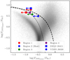 |
Fig. 8. BPT diagnostic diagram showing the flux ratios of the various emission regions for DELS J0411–0907 (squares) and VDES J0020–3653 (circles); the F[N II]λ6584 Å/FHα ratios are all upper limits due to a non-detection of [N II] λ6583. The different colours represent the different emission regions, following the colour scheme in Figs. 5 and 7. The flux ratios were measured from the BLR-subtracted cube. For reference, we show the Kauffmann et al. (2003, black dotted) and Kewley et al. (2001, black dashed) curves which attempt to differentiate between galaxies primarily ionised by star formation (lower left) and AGN (upper right) at low-z. We also show local sources from the SDSS (Abazajian et al. 2009) as the 2D histogram, for comparison. |
We found that for both quasars, the companion emission regions (Region 1 for DELS J0411–0907 and Regions 1, 3 and 4 for VDES J0020–3653) have log(F[O III]λ5007/FHβ) between 0.55 and 0.78. DELS J0411–0907 Region 1 lies within the region of the diagram typically populated by galaxies that are primarily ionised by star formation. The VDES J0020–3653 companion regions could lie in the star-forming regime or in the transition region, and Region 1 could also lie within the AGN regime, depending on the ratio F[N II]λ6584 Å/FHα, for which we only have upper limits due to a lack of [N II] λ6583 detected in our sources.
The quasar host galaxies (Region 2) have log(F[O III]λ5007/FHβ) = 0.85 and 0.48 for DELS J0411–0907 and VDES J0020–3653, with log(F[N II]λ6584 Å/FHα) < −0.77 and −0.48. For DELS J0411–0907 we found that the host lies in the upper left of the diagram, which is sparsely populated by low-z objects, although lies within the AGN-dominated regime according to the low-z Kewley et al. (2001) demarcation. For VDES J0020–3653, the quasar host lies within the low-z transition region or star-forming regime. Theoretical models predict that high-z AGN will reside in the left side of the BPT diagram, in the AGN regime that is sparsely populated at z = 0 as well in the star-forming regime, mainly due to their lower metallicities (see e.g. Feltre et al. 2016; Strom et al. 2017; Nakajima & Maiolino 2022; Hirschmann et al. 2023). This is consistent with our measurements for both quasar host galaxies. For further discussion on this topic, see Übler et al. (2023).
To accurately determine the primary photoionisation mechanism within these various regions, we would require either deeper observations for a [N II] λ6583 detection or tighter limit, or alternative line-ratio diagnostic methods. We could use a [S II] λλ6717, 6731-based diagnostic (e.g. Veilleux & Osterbrock 1987); however, [S II] λλ6717, 6731 emission was not detected for these quasars. For the integrated quasar spectrum, by integrating the corresponding ERR array across the expected location of the [S II] λ6717 line, assuming the same line width as the narrow Hα component (Table 1), and applying our aperture correction, we found F[SII]λ6717 < 2.8 × 10⁻¹⁸ erg s−1 cm−2 (3σ) for DELS J0411–0907. For VDES J0020–3653, this line is beyond the wavelength coverage of the detector. These lines are either very close to or just above the detectable wavelength range for this G395H/F290LP NIRSpec configuration, making accurate measurements difficult if a line was detected. We have also not detected any He IIλ4686 emission, which is particularly useful for distinguishing star formation and AGN dominated regions in the high-z Universe where metallicities are low (see e.g. Nakajima & Maiolino 2022; Übler et al. 2023). For the integrated quasar spectrum, following the same process for [S II] λ6717 but instead assuming the same line width as the narrow [O III] λ5007 component (Table 1), we found FHeIIλ4686 < 2.3 × 10⁻¹⁸ erg s−1 cm−2 (3σ) for DELS J0411–0907 and FHeIIλ4686 < 1.6 × 10⁻¹⁸ erg s−1 cm−2 (3σ) for VDES J0020–3653.
3.2.3. Dynamical masses and black hole–dynamical mass ratios
To calculate the dynamical masses of the various emission regions, we followed the method as in Decarli et al. (2018) for ALMA quasar host studies. Firstly, we assumed that each region is dispersion-dominated, with:
where R is the radius of the region, σ the integrated line width, and G the gravitational constant. As an alternative, we assumed that the regions are rotation-dominated thin discs, with:
where 0.75 FWHM scales the line FWHM to the width of the line at 20% of the peak as in Willott et al. (2015), and i is the inclination angle of the thin disc. Finally, we also considered the virial approximation
This commonly used scaling factor of five was found to be the optimal scaling factor when calibrated to a sample of 25 galaxies by Cappellari et al. (2006; see e.g. van der Wel et al. 2022, for further discussion). This estimate is a factor of 10/3 larger than Mdyn, dispersion by construction. As it is most common for high-z quasar host studies to assume a rotating disc geometry (e.g. Wang et al. 2013; Willott et al. 2015; Decarli et al. 2018), we chose our best dynamical mass estimate to be Mdyn, rotation.
To measure the radii, we fit a 2D Gaussian to the spatial distribution of the [O III] λ5007 emission from each region, and took R to be the σ of the semi-major axis; these values are described in Sect. 3.2.1. From this Gaussian fit we also measured the axis-ratio, b/a, from which we derived the inclination angle, i, via cos(i) = b/a. As above, we note that R and b/a have not been deconvolved by the PSF. For the emission line widths we took the GN [O III] λ5007 component, which is the brightest of the lines we have measured. We note that this line width represents the total dynamics of the gas, including rotation as well as non-rotational components such as dispersion and winds (see e.g. Wisnioski et al. 2018). We considered only the N&B quasar subtracted cube for this calculation, since otherwise the measurements could be skewed by the unresolved NLR regions around the quasar. The kinematics of this central NLR are not dominated by the larger-scale galaxy potential, thus this emission does not trace the dynamical mass. Considering only the N&B quasar subtracted cube ensures that we are measuring the spatially extended host regions and not the PSF shape, which is particularly important for the host regions (Region 2). The values used in these calculations and the resulting dynamical mass estimates are listed in Table 5.
Dynamical masses, and values used in their calculation, for the emission-line regions in DELS J0411–0907 (upper rows) and VDES J0020–3653 (lower rows), using the N&B quasar subtraction.
For DELS J0411–0907, for Region 1 we found a dynamical mass between 0.6 − 2.5 × 10¹⁰ M⊙, with a best estimate of  , from an inclination angle i = 45 ± 3°. For the host Region 2, we found that the rotational measure for the dynamical mass,
  , is larger than the two other estimates,
  and
and  , albeit with large uncertainties particularly due to the inclination angle,
  . This difference is due to our measured inclination angle for this region being relatively low, and so the inclination correction is relatively large. For their ALMA quasar host galaxies that are marginally resolved, and thus where their axis ratio could not be accurately measured, Willott et al. (2015) and Decarli et al. (2018) assumed an inclination of 55°, the median inclination of the resolved sources in Willott et al. (2015) and Wang et al. (2013). As our quasar hosts are difficult to measure, requiring the quasar subtraction, and they are interacting systems which complicates their structure, we are not confident in our inclination measurements. If we instead assumed the median i = 55°, the rotational dynamical mass is
  , similar to the virial estimate. For Region 2 of DELS J0411–0907, we therefore assumed a best dynamical mass estimate of
  . Region 3 cannot be well described by a 2D Gaussian, and so we could not perform our fit as for the other regions.
VDES J0020–3653 Region 1 also cannot be well described by a 2D Gaussian, due to contamination by the quasar host, and so we did not estimate its dynamical mass. For the VDES J0020–3653 host Region 2, we found a dynamical mass between 4.6 − 17 × 1010 M⊙, with a best estimate of  , from an inclination of
  . This is similar to the median inclination of the resolved sources in Willott et al. (2015) and Wang et al. (2013), i = 55°, which would reduce the value slightly to
  . Region 3 has dynamical mass estimates of 4.7 − 15 × 1010 M⊙, with our best estimate
  from an inclination of
  . For VDES J0020–3653 Region 4 we found a dynamical mass between 3.1 − 10 × 1010 M⊙, with a best estimate from Mdyn, rotation of
  with an inclination of i = 62 ± 9°.
We plot the dynamical mass–black hole mass relation in Fig. 9 for these two quasars. We found that both of our quasars lie above the local Kormendy & Ho (2013) black hole–stellar mass relation, although these are consistent within the scatter and uncertainties. Previous ALMA observations have found that luminous quasars generally lie above the local black hole–host relation, while lower luminosity quasars lie around or below the relation (see e.g. Willott et al. 2017; Izumi et al. 2019). Our luminous quasars lie above the relation, which is consistent with this existing picture, however a larger sample of high-z quasars is required to test this scenario with NIRSpec. For a true comparison to the local black hole–stellar mass relation, we require stellar and not dynamical masses.
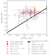 |
Fig. 9. Dynamical mass–black hole mass relation. Our two quasars DELS J0411–0907 (purple) and VDES J0020–3653 (orange) are shown, with the four Mdyn estimates, Mdyn, rotation, Mdyn, rotation assuming an inclination angle of 55°, Mdyn, dispersion and Mdyn, virial. The solid black hole mass error bars show the 1σ uncertainty on our best estimate of the black hole mass, while the transparent error bars very conservatively show the range of the lower limit of the lowest mass estimate to the upper limit of the largest mass estimate. The black line shows the local Kormendy & Ho (2013) relation. The grey points show a range of observations of high-z quasars as measured via their cold gas from ALMA (Willott et al. 2017; Izumi et al. 2018, 2019; Pensabene et al. 2020; Neeleman et al. 2021). |
We note that in the current observations the faint host galaxy continuum emission is not detectable, and so we could not measure their stellar masses. Our high spectral resolution (R ≃ 2700) observations were designed to study the emission lines in detail. This sacrifices the sensitivity that is required to detect the host continuum, which is expected to be achievable in similar exposure times at lower spectral resolution (either R ∼ 100 IFU spectra, or alternatively images as in e.g. Ding et al. 2023; Harikane et al. 2023). Future work within the GA-NIFS GTO programme will use the R ∼ 100 prism mode to search for the continuum emission of several high-z quasar host galaxies, which would make stellar mass measurements possible.
In Fig. 9 we also find that both of our quasars have dynamical masses and black hole–dynamical mass ratios consistent with ALMA observations of z ≳ 6 quasars. However, we note that DELS J0411–0907 and VDES J0020–3653 do not have published ALMA dynamical mass estimates that could be used for a direct comparison of these methods for our targets. A detailed comparison of ALMA and JWST NIRSpec dynamical mass and JWST stellar mass estimates will be a key aim of future quasar studies, which will allow for a much deeper understanding of the high-z black hole–host mass relations.
3.3. Outflow properties
The clear detection of an outflow component, as traced by the broad kinematic component (GB components in Fig. 2) via the analysis of the [O III] λ5007 velocity and spatial distribution, opens the possibility of investigating the ionised outflow properties in these early quasars. We note that this is the first time that it is possible to properly characterise the ionised outflows in quasars in the Epoch of Reionisation. Previous studies have relied on spatially unresolved information, and in particular on the detection of UV broad and blueshifted absorption features of UV resonant lines (e.g. Wang et al. 2018; Ginolfi et al. 2018; Onoue et al. 2019; Bischetti et al. 2022, 2023). These features trace primarily the nuclear outflow, which is generally a small fraction of the global, galactic scale outflow, and the lack of spatial information generally prevents a reliable estimate of the outflow parameters such as the outflow rate, kinetic power and momentum rate. We also note that NIRSpec fixed-slit spectroscopic observations of these two quasars covering the rest-frame UV do not reveal any broad absorption features (Willott, priv. comm.), indicating that the presence of ionised outflow is not necessarily traced by broad absorption features in the UV part of the spectrum (see e.g. Rankine et al. 2020).
In this work we have found outflow signatures within Hα, Hβ and [O III] λλ4959, 5007 for both quasars (GB components, Fig. 2). In this section we used the flux, velocity and spatial information of the Hβ and [O III] λ5007 broad galaxy (GB) components to infer some of the basic properties of the ionised outflow. We used the GB fluxes and velocities measured from our full integrated spectral fit for the quasar and host galaxy, prior to quasar subtraction, as described in Sect. 2.3.1 and shown in Fig. 2. This gives the most reliable measurements of the integrated quantities, as these are not affected by the quasar subtraction technique. To measure the spatial extent of the outflow, we used the quasar BLR-subtracted cube, from which we can measure the [O III] λ5007 line width in each spaxel without contamination from the quasar’s BLR. For this we considered the full cube, without splitting the emission into regions as in Sect. 3.2 above. The broad flux emanates from the quasar, approximately covering Region 2 for both quasars, as well as extending into Region 3 for DELS J0411–0907–this can be seen in the w80 maps in Fig. B.1.
To derive the mass of the ionised outflow as inferred from the blueshifted ‘outflow’ component of Hβ, we used the equation
from Carniani et al. (2015), assuming a density of the gas in the ionised outflow of ⟨ne⟩ = 500 cm−3, as in Carniani et al. (2015), and where C is a factor taking into account the clumpiness of the medium ( ), which we assume to be unity. Here we considered the LHβ to be the luminosity of the GB Hβ component as measured from our full integrated spectral fit for the quasar and host galaxy, as described in Sect. 2.3.1 and shown in Fig. 2. We note that as in our calculations above, we did not correct for extinction. We performed the equivalent calculation using the GB component of [O III] λ5007, using the corresponding equation from Carniani et al. (2015):
![$$ \begin{aligned} M_{\mathrm{out}} = 0.8\times 10^8 \frac{C}{10^{[\mathrm{O/H}] - [\mathrm{O/H}]_\odot }} \left(\frac{L_{[\mathrm{OIII}]}}{10^{44}\,\mathrm{erg\,s^{-1}}}\right) \left(\frac{\langle n_{\rm e}\rangle }{500\,\mathrm{cm}^{-3}}\right)^{-1}\,M_{\odot }, \end{aligned} $$](/articles/aa/full_html/2023/10/aa46113-23/aa46113-23-eq114.gif)
and assuming a solar oxygen abundance [O/H]=[O/H]⊙. These luminosities and calculated outflow masses are given in Table 6. By using the luminosities of the outflow component of Hβ we inferred outflow masses of ionised gas of  and
and  for DELS J0411–0907 and VDES J0020–3653, respectively. We note that the masses using the broad, blueshifted component of [O III] λ5007 are lower than the Hβ masses, by a factor of approximately two for DELS J0411–0907 and an order of magnitude for VDES J0020–3653. This is a well known issue and it is understood to be a consequence of the ionisation structure of the clouds in the NLR of AGNs, whereby the [O III] λ5007 only traces a small part of the mass of each cloud (e.g. Perna et al. 2015).
Once the outflow mass is inferred, the ionised outflow rate can be calculated under the thin shell approximation (which generally provides a better description of galactic outflow rates, relative to the uniformly filled outflows, as discussed in Lutz et al. 2020) by using the equation
where Rout is size of the outflow and vout is its velocity. To estimate Rout, we measured the maximum extent from the quasar centre of the [O III] λ5007 emission with w80 > 600 km s−1, in the BLR-subtracted cube. This w80 > 600 km s−1 is a conservative criterion that has been used in previous studies to classify outflows (e.g. Harrison et al. 2015; Kakkad et al. 2020). We note that for DELS J0411–0907 this outflow region extends from the host galaxy in Region 2 into Region 3, which is seen to have an outflow GB component in Fig. 5. For VDES J0020–3653, when we measured the maximum extent we excluded the south-south-west direction, avoiding the nearby Region 1 which may be artificially contributing to the large w80 values as its velocity is offset from the quasar. This Rout is a projected radius and it reproduces the true radius only if the directions of the outflow expansion include the plane of the sky. For the outflow velocity we adopted the same approach as Fluetsch et al. (2019) by defining vout = vpeak + vFWHM/2, where vpeak is the peak velocity of the GB component of [O III] λ5007 (and equivalently Hβ as they are kinematically tied in our spectral fits) and vFWHM its FWHM. These velocities are measured from our full integrated spectral fit for the quasar and host galaxy, which are given in Table 1. Our measured Rout and vout are given in Table 6. Based on these measured values we obtain ionised outflow rates from Hβ of  yr−1 and
  yr−1 for DELS J0411–0907 and VDES J0020–3653, respectively; the [O III] λ5007 rates are also quoted in Table 6.
We can also estimate the kinetic power of the outflows as
From the Hβ outflow, we obtain values of  erg s−1 and (51 ± 9)×1043 erg s−1 for DELS J0411–0907 and VDES J0020–3653, respectively, as given in Table 6.
The implications of these findings are discussed in Sect. 4.2.
4. Discussion
4.1. Quasar companions
Both of our quasars show additional emission-line regions nearby their host galaxies, which are consistent with being companion galaxies.
For DELS J0411–0907, Region 1 to the south-east of the quasar has a projected offset of ≃4.3 kpc from the quasar, with a widest extent of ≃8.8 kpc. From the integrated spectrum we found that this region has a velocity offset relative to the quasar host of −98 ± 72 km s−1, indicating minimal line-of-sight offset (Fig. 5 and Table 3). From the emission maps in Figs. 4 and B.1 we see that the velocity spans about 100 km s−1 either side of the host velocity. This companion galaxy is likely undergoing a merger with the quasar host. Region 3 exhibits some broader [O III] λλ4959, 5007 emission, indicating an ionised gas outflow in this region, and is likely a tidal tail.
For VDES J0020–3653, Region 1 to the south-south-west of the quasar has a projected offset of ≃2.8 kpc from the quasar, with a widest extent of ≃3.6 kpc. This region has a line-of-sight velocity offset by −55 ± 72 km s−1 from the host (Figs. 6 and B.1). Region 3 to the north-west of VDES J0020–3653 has a projected offset of ≃4.2 kpc from the quasar, with a widest extent of ≃4.6 kpc. This region has a line-of-sight velocity offset by +83 ± 72 km s−1 from the host, with the bulk of the gas at a similar offset. Region 4 to the south-west of the quasar has a projected offset of ≃5.6 kpc, and a widest extent of ≃4.8 kpc. This region has a line-of-sight velocity offset by +218 ± 72 km s−1 from the host, again with the bulk of this gas at a similar velocity.
All of these regions satisfy the common merger condition of having a projected distance of < 20 h−1 kpc, where h is the dimensionless Hubble constant h = H0/(100 km s−1 Mpc−1), and a velocity difference δV < 500 km s−1 (e.g. Patton et al. 2000; Conselice et al. 2009).
The presence of quasar companions, or lack thereof, provides important insights into quasar growth mechanisms. For example, theory predicts that kpc-scale interactions trigger AGN activity (e.g. Sanders et al. 1988; Hopkins et al. 2006), however mergers and companion galaxies are not ubiquitously observed around low-z quasars (Cisternas et al. 2011; Kocevski et al. 2012; Mechtley et al. 2016; Marian et al. 2019). However, these early quasars have more intense accretion, and higher merger rates are likely in the early Universe, suggesting that these mergers could be a key driver of this early black hole growth. ALMA observations have detected companion galaxies around high-z quasars at ≃8 − 60 kpc separations which are interpreted as major galaxy interactions (e.g. Wagg et al. 2012; Decarli et al. 2017), at rates of up to 50% in some samples (Trakhtenbrot et al. 2017; Nguyen et al. 2020). These companions are less frequently observed in the rest-frame UV (Willott et al. 2005), although some potential companions have been discovered with HST (McGreer et al. 2014; Marshall et al. 2020). The lack of UV-discovered companions may be due to dust obscuration (Trakhtenbrot et al. 2017), however our observations which reveal such close neighbours may indicate that resolution has previously limited our ability to identify merging quasars in the early Universe. It is indeed striking that both of our quasars have these companion galaxies, and it will be insightful to see whether other upcoming JWST observations also reveal similar structures around other high-z quasars, building up a larger statistical sample. Discovering these close companions highlights the ability of JWST to understand these early quasars in significantly greater detail, through detailed measurements of their environments and thus potential quasar triggering mechanisms (see also Perna et al. 2023).
4.2. Quasar driven outflows
In Fig. 10 we show the ionised outflow rate as a function of AGN luminosity for our two quasars at z ∼ 6.8, and for AGN whose ionised outflows had been measured at lower redshift (from the compilation of Fiore et al. 2017). Clearly, our two high-z quasars follow the same relation as lower redshift quasars.
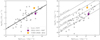 |
Fig. 10. Outflows of DELS J0411–0907 and VDES J0020–3653. Left: ionised gas outflow mass rate as a function of AGN luminosity, for the two quasars at z ∼ 6.8 presented in this paper, and for various other AGN at lower redshift (0 < z < 3; from Fiore et al. 2017). The solid line is a linear fit (in logarithmic scales) of the latter data. The ionised outflows of the two quasars at z ∼ 7 follow the same relation as quasars at lower redshifts. Right: kinetic power (PK) of the ionised outflows as a function of AGN luminosity (same symbols as in the left plot). The dashed lines show constant ratios of PK and LAGN as labelled. We note that the Fiore et al. (2017) galaxies have been shifted by log(5/2) for consistency with our density assumption of 500 cm−3, as they assume 200 cm−3. |
The inferred outflow rates (∼58 M⊙ yr−1 for DELS J0411–0907 and ∼525 M⊙ yr−1 for VDES J0020–3653) are significantly larger than the upper limits we have measured for the host SFRs (< 33 M⊙ yr−1 for DELS J0411–0907 and < 54 M⊙ yr−1 for VDES J0020–3653; see Sect. 3.2.2). These outflow rates are much larger than the SFRs, especially if we consider that the measured outflow rates are only for the ionised component and that the other phases, in particular the molecular phase, may also contribute. This result implies that, if prolonged, the quasar-driven outflow may be the main agent responsible for depleting the galaxy of its gas content. However, one has to take into account that the quasar activity is likely short lived and bursty, hence it may not continue for a time long enough to compete with star formation in depleting the gas mass.
More quantitative consideration on the potential feedback effect of the quasar driven outflow can be obtained by considering the kinetic power of the outflows. Efficient feedback, with high coupling with the ISM, in many scenarios requires that the kinetic power of the outflow should be about 5−7% of the AGN bolometric luminosity. The right panel of Fig. 10 shows the kinetic power of ionised outflows as a function of AGN luminosity, where locii of constant PK/LAGN ratio are also indicated with dashed lines. Clearly, the ionised outflows of two quasars at z ∼ 6.8 have a kinetic power that is less than 1% of LAGN (in the case of DELS J0411–0907 actually < 0.1%), indicating that the outflow may not be an effective feedback mechanism.
Moreover, the momentum rate (Ṁoutvout) of the two quasars is 0.07 LAGN/c and 1.28 LAGN/c for DELS J0411–0907 and VDES J0020–3653, respectively. These values are much lower than expected by the (very feedback-effective) energy-driven outflows, which expect a momentum boost by a factor of ∼20 relative to the radiation momentum rate LAGN/c. Based on these values, these outflows seem to be more consistent with momentum-driven outflows, possibly resulting from radiation pressure on the dusty clouds (Fabian 2012; Costa et al. 2014). However, once again, we caution that with our NIRSpec data we can only probe the ionised phase of these outflows. The other phases of the outflows, and in particular the molecular component, may be much more massive and energetic (Fluetsch et al. 2019), although Fiore et al. (2017) suggest that at such high luminosities the ionised outflows may be comparable or stronger than the other phases. Future deep observations with ALMA may provide constraints on the other phases of these outflows and, therefore, provide additional information on the feedback role of AGN-driven outflows in these two early quasars.
5. Conclusions
We have analysed JWST NIRSpec IFU observations of two z ≃ 6.8 quasars, DELS J0411–0907 and VDES J0020–3653. By analysing their integrated quasar spectrum, we measured black hole masses from the Hβ and Hα broad lines, which are the most reliable single-epoch mass estimators. These are some of the first observations of Balmer broad emission lines in high-z quasars, making such a measurement possible for the first time. We derived a best estimate for the black hole mass in DELS J0411–0907 of  , implying an Eddington ratio of
  . This is more massive than the Mg II mass estimates of MBH, MgII = (0.6 − 1)×109 M⊙ which implied more extreme Eddington ratios of λEdd = 1.3 − 2.4. By measuring a more accurate black hole mass, we have revised our understanding of the accretion physics of this early quasar. For VDES J0020–3653, our best estimate of the black hole mass is
  , corresponding to an Eddington ratio of
  . This is more consistent with the Mg II measurements of Reed et al. (2019). Together, these quasars show that the Mg II black hole mass can be significantly biased relative to the Hβ estimate for some high-z quasars, while for others these two techniques may give consistent black hole mass measurements, highlighting the benefit of measuring these more reliable Hβ masses.
We performed quasar subtraction on our IFU observations, by modelling the PSF using the variation in the flux of the quasar broad Hα and Hβ lines across the spatial domain. From this subtraction, we revealed that the host galaxy of DELS J0411–0907 shows emission extending to a radius of 2.5 kpc, described by a 2D Gaussian with semi-major axis σ = 0.75 kpc. This host has narrow [O III] λλ4959, 5007, Hβ, and Hα emission, alongside a broader wing emission from an outflow. We estimated that the host has a SFR of < 33 M⊙ yr−1, with a dynamical mass in the range of 2.6 − 16 × 1010 M⊙ with a best estimate of  . This host galaxy lies within the AGN-dominated regime of the low-z BPT diagram.
The host galaxy of VDES J0020–3653 has emission extending to a radius of 2.1 kpc, described by a 2D Gaussian with semi-major axis σ = 1.0 kpc. Both narrow [O III] λλ4959, 5007, Hβ, and Hα and broad-wing emission is detected. We estimated a SFR of < 54 M⊙ yr−1 for this host, with a dynamical mass between 4.6 − 17 × 1010 M⊙ with a best estimate of  . The host of VDES J0020–3653 lies within the star-forming or transition region of the low-z BPT diagram; however, this is likely due to the low metallicity of these quasar hosts, with low-metallicity, high-z AGN predicted to lie in this region.
We found that from our measured black hole and dynamical masses, DELS J0411–0907 and VDES J0020–3653 both lie slightly above the local black hole–host mass relation (Kormendy & Ho 2013) and are consistent with the existing observations of z ≳ 6 quasar host galaxies with ALMA. Both quasars are found to have additional emission-line regions near their host galaxies, with two regions for DELS J0411–0907 and three for VDES J0020–3653. We have studied these companion regions, measuring their SFRs, excitation mechanisms, and kinematics. We found that four companion regions are likely to be either galaxies merging with the quasar host galaxy, and one an extended tidal tail. It is striking that both of our high-z quasars are undergoing galaxy mergers, and it will be insightful to see the fraction of high-z quasars that are found to also have companions in future NIRSpec IFU observations.
We detect ionised outflows in [O III] λλ4959, 5007, and Hβ from both VDES J0020–3653 and DELS J0411–0907. We measured the rates of the ionised outflow from Hβ to be  yr−1 for DELS J0411–0907 and
  yr−1 for VDES J0020–3653. These outflow rates are much larger than the SFRs of the host galaxies, implying that if this is prolonged, the quasar-driven outflow may be the main driver for gas depletion within the galaxies. We found that these outflows are likely momentum-driven, and are not likely to be effective feedback mechanisms.
This work highlights the exquisite capabilities of the JWST NIRSpec IFU for observing high-z quasars. With the high-resolution spectral coverage in the infrared, we are able to study key rest-frame optical emission lines that have been previously unobservable, such as Hβ, [O III] λλ4959, 5007, and Hα. This has allowed us to measure the black hole masses and Eddington ratios of these quasars more accurately than had been previously possible. Obtaining spatially resolved IFU spectra has also allowed us to study the host galaxies, local environments, and outflow properties of these quasars in great detail. Overall, this work shows the possibilities of the NIRSpec IFU, and we look forward to the insights that this instrument will give about the formation and growth of quasars and their host galaxies in the early Universe.
Acknowledgments
We thank the anonymous referee for their constructive feedback which greatly improved the manuscript. We thank Bernd Husemann for his help with the QDeblend3D software and sharing his expertise on quasar subtraction. M.M. would like to thank Toby Brown for his helpful advice, particularly on creating the kinematic maps. This work is based on observations made with the NASA/ESA/CSA James Webb Space Telescope. The data were obtained from the Mikulski Archive for Space Telescopes at the Space Telescope Science Institute, which is operated by the Association of Universities for Research in Astronomy, Inc., under NASA contract NAS 5-03127 for JWST. These observations are associated with programme #1222, as part of the Galaxy Assembly with NIRSpec IFS GTO programme. M.A.M. acknowledges the support of a National Research Council of Canada Plaskett Fellowship, and the Australian Research Council Centre of Excellence for All Sky Astrophysics in 3 Dimensions (ASTRO 3D), through project number CE170100013. S.A., B.R.P. and M.P. acknowledge support from the research project PID2021-127718NB-I00 of the Spanish Ministry of Science and Innovation/State Agency of Research (MICIN/AEI). M.P. also acknowledges support from the Programa Atracción de Talento de la Comunidad de Madrid via grant 2018-T2/TIC-11715. R.M., J.S. and F.D.E. acknowledge support by the Science and Technology Facilities Council (STFC), from the ERC Advanced Grant 695671 ‘QUENCH’. R.M. and J.S. also acknowledge funding from a research professorship from the Royal Society. G.C. acknowledges the support of the INAF Large Grant 2022 ‘The metal circle: a new sharp view of the baryon cycle up to Cosmic Dawn with the latest generation IFU facilities’. H.Ü. gratefully acknowledges support by the Isaac Newton Trust and by the Kavli Foundation through a Newton-Kavli Junior Fellowship. A.J.B., G.C.J. and A.J.C. acknowledge funding from the ‘FirstGalaxies’ Advanced Grant from the European Research Council (ERC) under the European Union’s Horizon 2020 research and innovation programme (Grant agreement No. 789056). S.C. acknowledges support from the European Union (ERC, WINGS, 101040227). P.G.P.-G. acknowledges support from Spanish Ministerio de Ciencia e Innovación MCIN/AEI/10.13039/501100011033 through grant PGC2018-093499-B-I00. The Cosmic Dawn Center (DAWN) is funded by the Danish National Research Foundation under grant no. 140 This research has made use of NASA’s Astrophysics Data System, QFitsView, and SAOImageDS9, developed by Smithsonian Astrophysical Observatory. This paper made use of Python packages and software AstroPy (Astropy Collaboration 2013), Matplotlib (Hunter 2007), NumPy (van der Walt et al. 2011), Pandas (Pandas Development Team 2020), Photutils (Bradley et al. 2018), Regions (Bradley et al. 2022), SciPy (Virtanen et al. 2020), Seaborn (Waskom 2021), Spectral Cube (Ginsburg et al. 2019), QDeblend3D (Husemann et al. 2013, 2014), and QubeSpec (https://github.com/honzascholtz/Qubespec).
References
- Abazajian, K. N., Adelman-McCarthy, J. K., Agüeros, M. A., et al. 2009, ApJS, 182, 543 [Google Scholar]
- Astropy Collaboration (Robitaille, T. P., et al.) 2013, A&A, 558, A33 [NASA ADS] [CrossRef] [EDP Sciences] [Google Scholar]
- Baldwin, J. A., Phillips, M. M., & Terlevich, R. 1981, PASP, 93, 5 [Google Scholar]
- Banados, E., Schindler, J.-T., Venemans, B. P., et al. 2022, ApJS, 265, 29 [Google Scholar]
- Bañados, E., Venemans, B. P., Decarli, R., et al. 2016, ApJS, 227, 11 [Google Scholar]
- Bañados, E., Venemans, B. P., Mazzucchelli, C., et al. 2018, Nature, 553, 473 [Google Scholar]
- Bertoldi, F., Cox, P., Neri, R., et al. 2003, A&A, 409, L47 [NASA ADS] [CrossRef] [EDP Sciences] [Google Scholar]
- Bischetti, M., Feruglio, C., D’Odorico, V., et al. 2022, Nature, 605, 244 [NASA ADS] [CrossRef] [Google Scholar]
- Bischetti, M., Fiore, F., Feruglio, C., et al. 2023, ApJ, 952, 44 [NASA ADS] [CrossRef] [Google Scholar]
- Böker, T., Arribas, S., Lützgendorf, N., et al. 2022, A&A, 661, A82 [NASA ADS] [CrossRef] [EDP Sciences] [Google Scholar]
- Böker, T., Beck, T. L., Birkmann, S. M., et al. 2023, PASP, 135, 038001 [CrossRef] [Google Scholar]
- Bradley, L., Sipocz, B., Robitaille, T., et al. 2018, https://doi.org/10.5281/zenodo.1340699 [Google Scholar]
- Bradley, L., Deil, C., Ginsburg, A., et al. 2022, https://doi.org/10.5281/zenodo.7259631 [Google Scholar]
- Bruzual, G., & Charlot, S. 2003, MNRAS, 344, 1000 [NASA ADS] [CrossRef] [Google Scholar]
- Bushouse, H., Eisenhamer, J., Dencheva, N., et al. 2022, https://doi.org/10.5281/zenodo.7229890 [Google Scholar]
- Calzetti, D., Armus, L., Bohlin, R. C., et al. 2000, ApJ, 533, 682 [NASA ADS] [CrossRef] [Google Scholar]
- Cappellari, M., Bacon, R., Bureau, M., et al. 2006, MNRAS, 366, 1126 [Google Scholar]
- Carniani, S., Marconi, A., Maiolino, R., et al. 2015, A&A, 580, A102 [NASA ADS] [CrossRef] [EDP Sciences] [Google Scholar]
- Cisternas, M., Jahnke, K., Inskip, K. J., et al. 2011, ApJ, 726, 57 [NASA ADS] [CrossRef] [Google Scholar]
- Coatman, L., Hewett, P. C., Banerji, M., & Richards, G. T. 2016, MNRAS, 461, 647 [NASA ADS] [CrossRef] [Google Scholar]
- Conselice, C. J., Yang, C., & Bluck, A. F. L. 2009, MNRAS, 394, 1956 [NASA ADS] [CrossRef] [Google Scholar]
- Costa, T., Sijacki, D., & Haehnelt, M. G. 2014, MNRAS, 444, 2355 [Google Scholar]
- Cresci, G., Mainieri, V., Brusa, M., et al. 2015, ApJ, 799, 82 [Google Scholar]
- Decarli, R., Walter, F., Yang, Y., et al. 2012, ApJ, 756, 150 [NASA ADS] [CrossRef] [Google Scholar]
- Decarli, R., Walter, F., Venemans, B. P., et al. 2017, Nature, 545, 457 [Google Scholar]
- Decarli, R., Walter, F., Venemans, B. P., et al. 2018, ApJ, 854, 97 [Google Scholar]
- Ding, X., Onoue, M., Silverman, J. D., et al. 2023, Nature, 621, 51 [NASA ADS] [CrossRef] [Google Scholar]
- Domínguez, A., Siana, B., Henry, A. L., et al. 2013, ApJ, 763, 145 [CrossRef] [Google Scholar]
- Dunlop, J. S., McLure, R. J., Kukula, M. J., et al. 2003, MNRAS, 340, 1095 [NASA ADS] [CrossRef] [Google Scholar]
- Eilers, A.-C., Simcoe, R. A., Yue, M., et al. 2022, ApJ, 950, 68 [Google Scholar]
- Fabian, A. 2012, ARA&A, 50, 455 [CrossRef] [Google Scholar]
- Fan, X., White, R. L., Davis, M., et al. 2000, AJ, 120, 1167 [NASA ADS] [CrossRef] [Google Scholar]
- Fan, X., Narayanan, V. K., Lupton, R. H., et al. 2001, AJ, 122, 2833 [Google Scholar]
- Fan, X., Strauss, M. A., Schneider, D. P., et al. 2003, AJ, 125, 1649 [Google Scholar]
- Farina, E. P., Schindler, J.-T., Walter, F., et al. 2022, ApJ, 941, 106 [NASA ADS] [CrossRef] [Google Scholar]
- Feltre, A., Charlot, S., & Gutkin, J. 2016, MNRAS, 456, 3354 [Google Scholar]
- Fiore, F., Feruglio, C., Shankar, F., et al. 2017, A&A, 601, A143 [NASA ADS] [CrossRef] [EDP Sciences] [Google Scholar]
- Fluetsch, A., Maiolino, R., Carniani, S., et al. 2019, MNRAS, 483, 4586 [NASA ADS] [Google Scholar]
- Gardner, J. P., Mather, J. C., Clampin, M., et al. 2006, Space Sci. Rev., 123, 485 [Google Scholar]
- Gardner, J. P., Mather, J. C., Abbott, R., & Zondag, E. 2023, PASP, 135, 068001 [CrossRef] [Google Scholar]
- Ginolfi, M., Maiolino, R., Carniani, S., et al. 2018, MNRAS, 476, 2421 [NASA ADS] [CrossRef] [Google Scholar]
- Ginsburg, A., Koch, E., Robitaille, T., et al. 2019, https://doi.org/10.5281/zenodo.3558614 [Google Scholar]
- Greene, J. E., & Ho, L. C. 2005, ApJ, 630, 122 [NASA ADS] [CrossRef] [Google Scholar]
- Harikane, Y., Zhang, Y., Nakajima, K., et al. 2023, ArXiv e-prints [arXiv:2303.11946] [Google Scholar]
- Harrison, C. M., Alexander, D. M., Mullaney, J. R., et al. 2015, MNRAS, 456, 1195 [Google Scholar]
- Hinshaw, G., Larson, D., Komatsu, E., et al. 2013, ApJS, 208, 19 [Google Scholar]
- Hirschmann, M., Charlot, S., Feltre, A., et al. 2023, MNRAS, 526, 3610 [NASA ADS] [CrossRef] [Google Scholar]
- Hopkins, P. F., Hernquist, L., Cox, T. J., et al. 2006, ApJS, 163, 1 [Google Scholar]
- Hunter, J. D. 2007, Comput. Sci. Eng., 9, 90 [NASA ADS] [CrossRef] [Google Scholar]
- Husemann, B., Wisotzki, L., Sánchez, S. F., & Jahnke, K. 2013, A&A, 549, A43 [NASA ADS] [CrossRef] [EDP Sciences] [Google Scholar]
- Husemann, B., Jahnke, K., Sánchez, S. F., et al. 2014, MNRAS, 443, 755 [NASA ADS] [CrossRef] [Google Scholar]
- Hutchings, J. B. 2003, AJ, 125, 1053 [NASA ADS] [CrossRef] [Google Scholar]
- Izumi, T., Onoue, M., Shirakata, H., et al. 2018, PASJ, 70, 36 [NASA ADS] [Google Scholar]
- Izumi, T., Onoue, M., Matsuoka, Y., et al. 2019, PASJ, 71, 111 [CrossRef] [Google Scholar]
- Jakobsen, P., Ferruit, P., de Oliveira, C. A., et al. 2022, A&A, 661, A80 [NASA ADS] [CrossRef] [EDP Sciences] [Google Scholar]
- Kakkad, D., Mainieri, V., Vietri, G., et al. 2020, A&A, 642, A147 [NASA ADS] [CrossRef] [EDP Sciences] [Google Scholar]
- Kashikawa, N., Ishizaki, Y., Willott, C. J., et al. 2015, ApJ, 798, 28 [Google Scholar]
- Kashino, D., Lilly, S. J., Matthee, J., et al. 2022, ApJ, 950, 66 [Google Scholar]
- Kaspi, S., Smith, P. S., Netzer, H., et al. 2000, ApJ, 533, 631 [Google Scholar]
- Kaspi, S., Brandt, W. N., Maoz, D., et al. 2021, ApJ, 915, 129 [NASA ADS] [CrossRef] [Google Scholar]
- Kauffmann, G., Heckman, T. M., Tremonti, C., et al. 2003, MNRAS, 346, 1055 [Google Scholar]
- Kennicutt, R. C. 1998, ARA&A, 36, 189 [NASA ADS] [CrossRef] [Google Scholar]
- Kennicutt, R. C., & Evans, N. J. 2012, ARA&A, 50, 531 [NASA ADS] [CrossRef] [Google Scholar]
- Kewley, L. J., Dopita, M. A., Sutherland, R. S., Heisler, C. A., & Trevena, J. 2001, ApJ, 556, 121 [Google Scholar]
- Kocevski, D. D., Faber, S. M., Mozena, M., et al. 2012, ApJ, 744, 148 [NASA ADS] [CrossRef] [Google Scholar]
- Kormendy, J., & Ho, L. C. 2013, ARA&A, 51, 511 [Google Scholar]
- Kovacevic, J., Popovic, L. C., & Dimitrijevic, M. S. 2010, ApJS, 189, 15 [CrossRef] [Google Scholar]
- Kuraszkiewicz, J. K., Green, P. J., Forster, K., et al. 2002, ApJS, 143, 257 [NASA ADS] [CrossRef] [Google Scholar]
- Law, D. D., Morrison, J. E., Argyriou, I., et al. 2023, AJ, 166, 45 [NASA ADS] [CrossRef] [Google Scholar]
- Lee, J. C., de Paz, A. G., Tremonti, C., et al. 2009, ApJ, 706, 599 [NASA ADS] [CrossRef] [Google Scholar]
- Lutz, D., Sturm, E., Janssen, A., et al. 2020, A&A, 633, A134 [NASA ADS] [CrossRef] [EDP Sciences] [Google Scholar]
- Marian, V., Jahnke, K., Mechtley, M., et al. 2019, ApJ, 882, 141 [CrossRef] [Google Scholar]
- Marshall, M. A., Mechtley, M., Windhorst, R. A., et al. 2020, ApJ, 900, 21 [NASA ADS] [CrossRef] [Google Scholar]
- Marshall, M. A., Wyithe, J. S. B., Windhorst, R. A., et al. 2021, MNRAS, 506, 1209 [CrossRef] [Google Scholar]
- Matsuoka, Y., Onoue, M., Kashikawa, N., et al. 2018, PASJ, 70, S10 [NASA ADS] [CrossRef] [Google Scholar]
- McElwain, M. W., Feinberg, L. D., Perrin, M. D., et al. 2023, PASP, 135, 058001 [NASA ADS] [CrossRef] [Google Scholar]
- McGreer, I. D., Fan, X., Strauss, M. A., et al. 2014, AJ, 148, 73 [NASA ADS] [CrossRef] [Google Scholar]
- McLeod, K. K., & Rieke, G. H. 1994, ApJ, 420, 58 [CrossRef] [Google Scholar]
- Mechtley, M., Windhorst, R. A., Ryan, R. E., et al. 2012, ApJ, 756, L38 [NASA ADS] [CrossRef] [Google Scholar]
- Mechtley, M., Jahnke, K., Windhorst, R. A., et al. 2016, ApJ, 830, 156 [NASA ADS] [CrossRef] [Google Scholar]
- Nagao, T., Marconi, A., & Maiolino, R. 2006, A&A, 447, 157 [NASA ADS] [CrossRef] [EDP Sciences] [Google Scholar]
- Nakajima, K., & Maiolino, R. 2022, MNRAS, 513, 5134 [NASA ADS] [CrossRef] [Google Scholar]
- Neeleman, M., Novak, M., Venemans, B. P., et al. 2021, ApJ, 911, 141 [NASA ADS] [CrossRef] [Google Scholar]
- Nguyen, N. H., Lira, P., Trakhtenbrot, B., et al. 2020, ApJ, 895, 74 [NASA ADS] [CrossRef] [Google Scholar]
- Onoue, M., Kashikawa, N., Matsuoka, Y., et al. 2019, ApJ, 880, 77 [Google Scholar]
- Osterbrock, D. E. 1989, Astrophysics of Gaseous Nebulae and Active Galactic Nuclei (Mill Valley: University Science Books) [Google Scholar]
- Pandas Development Team 2020, https://doi.org/10.5281/zenodo.3509134 [Google Scholar]
- Patton, D. R., Carlberg, R. G., Marzke, R. O., et al. 2000, ApJ, 536, 153 [NASA ADS] [CrossRef] [Google Scholar]
- Pensabene, A., Carniani, S., Perna, M., et al. 2020, A&A, 637, A84 [NASA ADS] [CrossRef] [EDP Sciences] [Google Scholar]
- Perna, M., Brusa, M., Cresci, G., et al. 2015, A&A, 574, A82 [NASA ADS] [CrossRef] [EDP Sciences] [Google Scholar]
- Perna, M., Arribas, S., Marshall, M., et al. 2023, A&A, accepted [arXiv:2304.06756] [Google Scholar]
- Peterson, B. M. 2009, Proc. Int. Astron. Union, 5, 151 [CrossRef] [Google Scholar]
- Pons, E., McMahon, R. G., Simcoe, R. A., et al. 2019, MNRAS, 484, 5142 [NASA ADS] [CrossRef] [Google Scholar]
- Rankine, A. L., Hewett, P. C., Banerji, M., & Richards, G. T. 2020, MNRAS, 492, 4553 [CrossRef] [Google Scholar]
- Reed, S. L., Banerji, M., Becker, G. D., et al. 2019, MNRAS, 487, 1874 [Google Scholar]
- Riechers, D. A., Walter, F., Carilli, C. L., & Bertoldi, F. 2007, ApJ, 671, L13 [NASA ADS] [CrossRef] [Google Scholar]
- Rigby, J., Perrin, M., McElwain, M., et al. 2022, PASP, 135, 048001 [Google Scholar]
- Sanders, D. B., Soifer, B. T., Elias, J. H., et al. 1988, ApJ, 325, 74 [Google Scholar]
- Schmidt, M. 1963, Nature, 197, 1040 [Google Scholar]
- Shen, Y., & Kelly, B. C. 2012, ApJ, 746, 169 [NASA ADS] [CrossRef] [Google Scholar]
- Shen, Y., Greene, J. E., Strauss, M. A., Richards, G. T., & Schneider, D. P. 2008, ApJ, 680, 169 [Google Scholar]
- Shen, Y., Richards, G. T., Strauss, M. A., et al. 2011, ApJS, 194, 45 [Google Scholar]
- Sijacki, D., Springel, V., & Haehnelt, M. G. 2009, MNRAS, 400, 100 [NASA ADS] [CrossRef] [Google Scholar]
- Strom, A. L., Steidel, C. C., Rudie, G. C., et al. 2017, ApJ, 836, 164 [NASA ADS] [CrossRef] [Google Scholar]
- Sun, J. 2020, Sun_Astro_Tools, GitHub [Google Scholar]
- Sun, J., Leroy, A. K., Schruba, A., et al. 2018, ApJ, 860, 172 [NASA ADS] [CrossRef] [Google Scholar]
- Trakhtenbrot, B., Lira, P., Netzer, H., et al. 2017, ApJ, 836, 8 [NASA ADS] [CrossRef] [Google Scholar]
- Trevese, D., Perna, M., Vagnetti, F., Saturni, F. G., & Dadina, M. 2014, ApJ, 795, 164 [NASA ADS] [CrossRef] [Google Scholar]
- Übler, H., Maiolino, R., Curtis-Lake, E., et al. 2023, A&A, 677, A145 [NASA ADS] [CrossRef] [EDP Sciences] [Google Scholar]
- van der Walt, S., Colbert, S. C., & Varoquaux, G. 2011, Comput. Sci. Eng., 13, 22 [Google Scholar]
- van der Wel, A., van Houdt, J., Bezanson, R., et al. 2022, ApJ, 936, 9 [NASA ADS] [CrossRef] [Google Scholar]
- van Dokkum, P. G. 2001, PASP, 113, 1420 [Google Scholar]
- Vayner, A., Wright, S. A., Do, T., et al. 2016, ApJ, 821, 64 [NASA ADS] [CrossRef] [Google Scholar]
- Veilleux, S., & Osterbrock, D. E. 1987, ApJS, 63, 295 [Google Scholar]
- Venemans, B. P., Walter, F., Zschaechner, L., et al. 2015, ApJ, 816, 37 [CrossRef] [Google Scholar]
- Venemans, B. P., Walter, F., Decarli, R., et al. 2017, ApJ, 837, 146 [NASA ADS] [CrossRef] [Google Scholar]
- Vestergaard, M., & Osmer, P. S. 2009, ApJ, 699, 800 [Google Scholar]
- Vestergaard, M., & Peterson, B. M. 2006, ApJ, 641, 689 [Google Scholar]
- Virtanen, P., Gommers, R., Oliphant, T. E., et al. 2020, Nat. Meth., 17, 261 [Google Scholar]
- Volonteri, M., & Rees, M. J. 2005, ApJ, 633, 624 [NASA ADS] [CrossRef] [Google Scholar]
- Volonteri, M., Silk, J., & Dubus, G. 2015, ApJ, 804, 148 [Google Scholar]
- Wagg, J., Wiklind, T., Carilli, C. L., et al. 2012, ApJ, 752, L30 [NASA ADS] [CrossRef] [Google Scholar]
- Walter, F., Bertoldi, F., Carilli, C., et al. 2003, Nature, 424, 406 [Google Scholar]
- Walter, F., Carilli, C., Bertoldi, F., et al. 2004, ApJ, 615, L17 [NASA ADS] [CrossRef] [Google Scholar]
- Walter, F., Neeleman, M., Decarli, R., et al. 2022, ApJ, 927, 21 [NASA ADS] [CrossRef] [Google Scholar]
- Wandel, A., Peterson, B. M., & Malkan, M. A. 1999, ApJ, 526, 579 [NASA ADS] [CrossRef] [Google Scholar]
- Wang, R., Carilli, C. L., Neri, R., et al. 2010, ApJ, 714, 699 [Google Scholar]
- Wang, R., Wagg, J., Carilli, C. L., et al. 2011, AJ, 142, 101 [NASA ADS] [CrossRef] [Google Scholar]
- Wang, R., Wagg, J., Carilli, C. L., et al. 2013, ApJ, 773, 44 [Google Scholar]
- Wang, F., Yang, J., Fan, X., et al. 2018, ApJ, 869, L9 [NASA ADS] [CrossRef] [Google Scholar]
- Wang, F., Yang, J., Fan, X., et al. 2019, ApJ, 884, 30 [Google Scholar]
- Waskom, M. 2021, J. Open Source Softw., 6, 3021 [CrossRef] [Google Scholar]
- Willott, C. J., Percival, W. J., McLure, R. J., et al. 2005, ApJ, 626, 657 [NASA ADS] [CrossRef] [Google Scholar]
- Willott, C. J., Delorme, P., Reylé, C., et al. 2009, AJ, 137, 3541 [Google Scholar]
- Willott, C. J., Albert, L., Arzoumanian, D., et al. 2010, AJ, 140, 546 [NASA ADS] [CrossRef] [Google Scholar]
- Willott, C. J., Bergeron, J., & Omont, A. 2015, ApJ, 801, 123 [NASA ADS] [CrossRef] [Google Scholar]
- Willott, C. J., Bergeron, J., & Omont, A. 2017, ApJ, 850, 108 [Google Scholar]
- Wisnioski, E., Mendel, J. T., Schreiber, N. M. F., et al. 2018, ApJ, 855, 97 [NASA ADS] [CrossRef] [Google Scholar]
- Wu, X.-B., Wang, F., Fan, X., et al. 2015, Nature, 518, 512 [Google Scholar]
- Yang, J., Wang, F., Fan, X., et al. 2021, ApJ, 923, 262 [NASA ADS] [CrossRef] [Google Scholar]
- Yang, J., Fan, X., Gupta, A., et al. 2023a, AAS, submitted [arXiv:2302.01777] [Google Scholar]
- Yang, J., Wang, F., Fan, X., et al. 2023b, ApJ, 951, L5 [NASA ADS] [CrossRef] [Google Scholar]
- Zakamska, N. L., & Greene, J. E. 2014, MNRAS, 442, 784 [Google Scholar]
Appendix A: Measured PSFs
The measured PSFs from the N&B quasar subtraction, for both Hα and Hβ, are shown for the two quasars in Figure A.1. We note that for VDES J0020–3653 the PSF shape does not follow the typical expected 6-pointed JWST PSF. This data cube is a combination of two separate observations taken at different position angles, 160.169 and 188.177 degrees, and so the resulting PSF of this combined cube would theoretically be two of the standard 6-point PSFs superimposed, one rotated by 28 degrees.
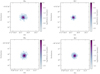 |
Fig. A.1. PSFs measured from the broad Hα and Hβ lines from DELS J0411–0907 (top) and VDES J0020–3653 (bottom), from the N&B quasar subtraction, as described in Section 2.3.3. These were created from the best fit quasar cube, which is the peak quasar spectrum scaled in flux to match the observed broad line flux in each spaxel. The relative intensity here depicts this scaling factor, which is the amount of flux in each spaxel relative to the brightest spaxel. We created two PSFs for each quasar, one from each of Hα and Hβ, as the PSF varies with wavelength. |
As the quasar subtraction technique measures the PSF from the data cube itself, and does not rely on PSF models, this does not affect our results. We have performed the quasar subtraction separately on both halves of the observation as a test, and verify that the host and companion features appear in both halves and are not distorted by this combination.
Appendix B: Kinematic maps using the BLR subtraction technique
Our kinematic maps for DELS J0411–0907 and VDES J0020–3653 as measured from the BLR quasar subtracted cubes are shown in Figure B.1. This can be compared to Figures 4 and Figures 6, which show the equivalent maps for the N&B quasar subtracted cubes for DELS J0411–0907 and VDES J0020–3653 respectively.
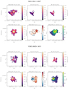 |
Fig. B.1. Kinematic maps for DELS J0411–0907 (top) and VDES J0020–3653 (bottom), after the subtraction of the quasar emission using the BLR subtraction technique. The top panels show the flux of the narrow component of the [O III] λ5007, Hβ, and Hα lines (GN), as fit by a Gaussian. The [O III] λ4959 line is not shown as it was constrained to have an amplitude three times fainter than that of [O III] λ5007. The bottom left panel shows the flux of the broader GB component of the [O III] λ5007 line, a second Gaussian with a larger σ. The lower middle and right panels show our kinematic maps, showing the non-parametric central velocity of the line (v50; middle) and the line width (w80; right). As these are non-parametric, this combines both the GN and GB components. We describe our method for creating these maps in Section 2.3.4. The black ellipses in the lower middle panels depict the regions as in Figures 5 and 7. |
Appendix C: Data cubes with pixel sub-sampling
Throughout this work we used data cubes with the native spaxel spatial size of 0.1″/pix, produced using the EMSM weighting to combine the various dither positions. With our dithering strategy it is also possible to sub-sample the data down to a pixel size of 0.05″/pix, to improve the spatial resolution which is limited by the pixel scale. For the best possible spatial resolution, we used cubes with a pixel scale of 0.05″ that have been combined using the drizzle weighting. This weighting optimises the resolution, but is more affected by the PSF effects (see Perna et al. 2023, for details). These 0.05″/pix drizzle cubes are highly affected by the PSF oscillations and chromatic effects, which we found result in very poor results for the quasar subtraction. Because the 0.1″/pix pixels optimise the S/N, and, most critically, give significantly improved results for the quasar subtraction that is the focus of our work, we used these 0.1″/pix EMSM cubes throughout this paper.
However, the 0.05″/pix drizzle cubes are more optimal for looking at the structural or morphological properties beyond the quasar host galaxy itself. In Figure C.1 we show the [O III] λ5007 flux maps for DELS J0411–0907 and VDES J0020–3653 using cubes that have been produced with 0.05″ pixels, combined using the drizzle weighting, following the method described in detail in Perna et al. (2023). This shows the companion galaxy morphology in greater detail. We found that in general, the morphology is consistent with our results from the 0.1″/pix cubes, showing a companion to the south-east of DELS J0411–0907 with a potential outflow to the north-west, and the two companion regions to the west of VDES J0020–3653.
 |
Fig. C.1. [O III] λ5007 flux maps for DELS J0411–0907 (left) and VDES J0020–3653 (right) using data cubes that have been produced with 0.05″/pix pixels, combined using the drizzle weighting, following the method described in detail in Perna et al. (2023). These maps were made using the original, non-continuum subtracted cubes. The stacked red, green, and blue images depict the integral of the flux across each of the specified wavelength or velocity windows, relative to the quasar redshift. The quasar peak location is marked as a black cross. |
One key difference is that the higher spatial resolution data for VDES J0020–3653 reveals a second distinct peak in the [O III] λ5007 emission, separated by only ∼0.37″ or 2 kpc (quasar peak to companion peak) to the south-south-west of the quasar. This very nearby companion, with a velocity offset by -179 km/s from the host Region 2 (GN), or -30 km/s with respect to the quasar’s peak [O III] λ5007 emission at z = 6.854, would be significantly interacting with the quasar host galaxy. This is so close to the quasar host that in the 0.1″/pix cubes this appears to be one elongated galaxy. Thus, if this region is not considered separately, and instead one elongated ellipse for this full emission region was chosen, we would overestimate the fluxes of the host galaxy of VDES J0020–3653. To account for this, we used the structure seen in Figure C.1 to define our region ellipses as seen in Figure 7, which we used to extract and thus analyse the individual regions’ spectra.
As we could not perform a reliable quasar subtraction on the higher resolution cubes, we did not use the cubes throughout this work. Our results focus on the host detection and thus require an accurate quasar subtraction.
All Tables
Measured line velocity offsets and velocity dispersions (relative to the quoted redshift) from the integrated quasar spectra.
Fluxes and luminosities measured for the 5100 Å continuum, Hα and Hβ BLR lines, alongside the derived black hole masses and Eddington ratios using these properties.
Flux ratios, SFRs, dust properties, and dust-corrected SFRs for the emission-line regions in DELS J0411–0907 (upper rows) and VDES J0020–3653 (lower rows).
Dynamical masses, and values used in their calculation, for the emission-line regions in DELS J0411–0907 (upper rows) and VDES J0020–3653 (lower rows), using the N&B quasar subtraction.
All Figures
|
Fig. 1. Quasar spectrum for DELS J0411–0907 (top) and VDES J0020–3653 (bottom), showing the spectrum from the brightest spaxel (navy), alongside the integrated spectrum (orange). The integrated spectrum was integrated over a radius of 0.35″ for the wavelengths bluewards of the detector gap, and 0.45″ redwards of the gap, corresponding to the apertures selected for our quasar fitting (Sect. 2.3.1). Our flux corrections of 81.4% and 86.6% have been applied to the integrated spectrum. The spectrum of the brightest spaxel is increased by a constant scaling factor, 8.230 for DELS J0411–0907 and 9.354 for VDES J0020–3653, such that the peak of Hα is equal for both spectra in the plots. The lower panel in each shows the spectra after continuum subtraction. For the brightest spaxel spectrum, the continuum model subtracted from the spectrum is shown in black in the top panel. For the continuum-subtracted integrated spectrum in the lower panel, the integration was performed on the continuum-subtracted cube (i.e. the continuum subtraction was first performed on each of the spaxels individually). The dotted grey vertical lines depict lines of interest at the redshift of the quasar (z = 6.854 for VDES J0020–3653 and z = 6.818 for DELS J0411–0907), and the grey regions show the continuum windows. The detector gap from 4.06 to 4.17 μm has been masked. We note that some minor oscillations are present in the single spaxel spectrum (navy), which can be particularly noticed below 3.3 μm in the single spaxel spectrum. These are caused by spatial undersampling of the PSF, which is a known issue when considering spectra in individual NIRSpec IFU spaxels; we describe this in detail in Perna et al. (2023). When measuring the quasar properties in Sect. 3.1, we used the integrated spectrum (orange), thus removing these single pixel effects. For the quasar subtraction, we found the best performance using the single spaxel spectrum (navy), however these oscillations do not significantly affect our results which directly focus on the regions around Hα and Hβ. |
| In the text | |
|
Fig. 2. Integrated quasar spectra for DELS J0411–0907 (top) and VDES J0020–3653 (bottom) (orange curve), showing the regions around Hβ (left) and Hα (right). The integrated spectrum was integrated over a radius of 0.35″ for the wavelengths bluewards of the detector gap, and 0.45″ redwards of the gap, corresponding to the apertures selected for our quasar fitting (Sect. 2.3.1). No flux correction has been applied. The best model fit (black) is shown alongside the narrow GN line components (green dot-dashed), the broader GB components (blue dashed lines), and the broken power law component for the BLR (red dotted lines). The lower panels show the residual of the model fit. |
| In the text | |
|
Fig. 3. Visualisation of the quasar subtraction using the broad Hβ (left) and Hα (right) lines from DELS J0411–0907. This shows the spectrum in spaxel (23, 24), with the quasar peak located at spaxel (26, 24), in image coordinates. The orange spectrum is the original continuum-subtracted spectrum in the spaxel, containing line flux from both the quasar and host galaxy. The black line is the quasar model spectrum. The top panels show the choice that the quasar model spectrum is that of the central brightest quasar spaxel, which contains both narrow and broad emission – the N&B subtraction. The bottom panel shows the choice that the quasar model spectrum is the BLR component from our best-fit model to the quasar spectrum (Fig. 2) – the BLR subtraction. Using the broad spectral windows marked in grey, the quasar model (black) was scaled to fit the combined spectrum (orange). The purple spectrum shows the residual to that fit, which is the host spectrum. |
| In the text | |
|
Fig. 4. Flux and kinematic maps for DELS J0411–0907, after the subtraction of the quasar emission using the N&B subtraction technique. The top panels show the flux of the narrow component of the [O III] λ5007, Hβ, and Hα lines (GN), as fit by a Gaussian. The bottom left panel shows the flux of the broader GB component of the [O III] λ5007 line, a second Gaussian with a larger σ. The lower middle and right panels show our kinematic maps, showing the non-parametric central velocity of the line (v50; middle) and the line width (w80; right). As these are non-parametric, this combines both the GN and GB components. We describe our method for creating these maps in Sect. 2.3.4. The black ellipses in the lower middle panel depict the regions as in Fig. 5. |
| In the text | |
|
Fig. 5. Emission line regions surrounding DELS J0411–0907. Top: the [O III] λ5007 flux map for DELS J0411–0907 after N&B quasar subtraction, with three regions of interest marked. Bottom: the integrated spectrum for the three regions (coloured lines), along with our best fit model in black. The middle panel, for Region 2, also shows the integrated spectra from the BLR quasar subtraction, in cyan, with the best fit model in grey. This region is the host of the quasar (position marked as a cyan cross in the top panel), and so the residual spectrum in this region depends heavily on the type of quasar subtraction. For Regions 1 and 3 the spectrum for both subtraction methods look equivalent, and so the BLR-subtracted spectra are not shown. For Region 2, we exclude the central nine pixels surrounding the quasar peak, as these are highly corrupted by the quasar subtraction and introduce significant noise and artefacts. This means that we slightly underestimate the total flux in this region; however, the fluxes are significantly more reliable than if these nine most corrupted spaxels were included. In Region 1, the spectral lines can be described by a single narrow Gaussian (GN), whereas in Regions 2 and 3 there is also a broader component fit with a second Gaussian (GB); these separate components can be seen as the dashed black lines for the N&B quasar subtraction, and dotted grey lines for the BLR quasar subtraction. |
| In the text | |
|
Fig. 6. Kinematic maps for VDES J0020–3653, after the subtraction of the quasar emission using the N&B subtraction technique. The top panels show the flux of the narrow component of the [O III] λ5007, Hβ, and Hα lines (GN), as fit by a Gaussian. The bottom left panel shows the flux of the broader GB component of the [O III] λ5007 line, a second Gaussian with a larger σ. The lower middle and right panels show our kinematic maps, showing the non-parametric central velocity of the line (v50; middle) and the line width (w80; right). As these are non-parametric, this combines both the GN and GB components. We describe our method for creating these maps in Sect. 2.3.4. The black ellipses in the lower middle panel depict the regions as in Fig. 7. |
| In the text | |
|
Fig. 7. Emission line regions surrounding VDES J0020–3653. Top: the [O III] λ5007 flux map for VDES J0020–3653 after N&B quasar subtraction, with four regions of interest marked. Bottom: the integrated spectrum for the four regions (coloured lines), along with our best fit model in black. The middle panel, for Region 2, also shows the integrated spectra from the BLR quasar subtraction, in cyan, with the best fit model in grey. This region is the host of the quasar (position marked as a cyan cross in the top panel), and so the residual spectrum in this region depends heavily on the type of quasar subtraction. We note that to account for the overlapping area between Regions 1 and 2, we assigned the flux in those spaxels to Region 1 only. For Region 2, we excluded the central nine pixels surrounding the quasar peak, as these are highly corrupted by the quasar subtraction and introduce significant noise and artefacts. This means that we slightly underestimate the total flux in this region, however the fluxes are significantly more reliable than if these nine most corrupted spaxels were included. In Regions 1, 3, and 4, the spectral lines can be described by a single narrow Gaussian (GN), whereas in Region 2 there is also a broader component which we fit with a second Gaussian (GB); these separate components can be seen as the dashed black lines for the N&B quasar subtraction, and dotted grey lines for the BLR quasar subtraction. We note that the emission around 3.8 μm in Regions 3 and 4 is likely an artefact in the cube. We did not see any significant detection of [N II] λλ6548, 6583. |
| In the text | |
|
Fig. 8. BPT diagnostic diagram showing the flux ratios of the various emission regions for DELS J0411–0907 (squares) and VDES J0020–3653 (circles); the F[N II]λ6584 Å/FHα ratios are all upper limits due to a non-detection of [N II] λ6583. The different colours represent the different emission regions, following the colour scheme in Figs. 5 and 7. The flux ratios were measured from the BLR-subtracted cube. For reference, we show the Kauffmann et al. (2003, black dotted) and Kewley et al. (2001, black dashed) curves which attempt to differentiate between galaxies primarily ionised by star formation (lower left) and AGN (upper right) at low-z. We also show local sources from the SDSS (Abazajian et al. 2009) as the 2D histogram, for comparison. |
| In the text | |
|
Fig. 9. Dynamical mass–black hole mass relation. Our two quasars DELS J0411–0907 (purple) and VDES J0020–3653 (orange) are shown, with the four Mdyn estimates, Mdyn, rotation, Mdyn, rotation assuming an inclination angle of 55°, Mdyn, dispersion and Mdyn, virial. The solid black hole mass error bars show the 1σ uncertainty on our best estimate of the black hole mass, while the transparent error bars very conservatively show the range of the lower limit of the lowest mass estimate to the upper limit of the largest mass estimate. The black line shows the local Kormendy & Ho (2013) relation. The grey points show a range of observations of high-z quasars as measured via their cold gas from ALMA (Willott et al. 2017; Izumi et al. 2018, 2019; Pensabene et al. 2020; Neeleman et al. 2021). |
| In the text | |
|
Fig. 10. Outflows of DELS J0411–0907 and VDES J0020–3653. Left: ionised gas outflow mass rate as a function of AGN luminosity, for the two quasars at z ∼ 6.8 presented in this paper, and for various other AGN at lower redshift (0 < z < 3; from Fiore et al. 2017). The solid line is a linear fit (in logarithmic scales) of the latter data. The ionised outflows of the two quasars at z ∼ 7 follow the same relation as quasars at lower redshifts. Right: kinetic power (PK) of the ionised outflows as a function of AGN luminosity (same symbols as in the left plot). The dashed lines show constant ratios of PK and LAGN as labelled. We note that the Fiore et al. (2017) galaxies have been shifted by log(5/2) for consistency with our density assumption of 500 cm−3, as they assume 200 cm−3. |
| In the text | |
|
Fig. A.1. PSFs measured from the broad Hα and Hβ lines from DELS J0411–0907 (top) and VDES J0020–3653 (bottom), from the N&B quasar subtraction, as described in Section 2.3.3. These were created from the best fit quasar cube, which is the peak quasar spectrum scaled in flux to match the observed broad line flux in each spaxel. The relative intensity here depicts this scaling factor, which is the amount of flux in each spaxel relative to the brightest spaxel. We created two PSFs for each quasar, one from each of Hα and Hβ, as the PSF varies with wavelength. |
| In the text | |
|
Fig. B.1. Kinematic maps for DELS J0411–0907 (top) and VDES J0020–3653 (bottom), after the subtraction of the quasar emission using the BLR subtraction technique. The top panels show the flux of the narrow component of the [O III] λ5007, Hβ, and Hα lines (GN), as fit by a Gaussian. The [O III] λ4959 line is not shown as it was constrained to have an amplitude three times fainter than that of [O III] λ5007. The bottom left panel shows the flux of the broader GB component of the [O III] λ5007 line, a second Gaussian with a larger σ. The lower middle and right panels show our kinematic maps, showing the non-parametric central velocity of the line (v50; middle) and the line width (w80; right). As these are non-parametric, this combines both the GN and GB components. We describe our method for creating these maps in Section 2.3.4. The black ellipses in the lower middle panels depict the regions as in Figures 5 and 7. |
| In the text | |
|
Fig. C.1. [O III] λ5007 flux maps for DELS J0411–0907 (left) and VDES J0020–3653 (right) using data cubes that have been produced with 0.05″/pix pixels, combined using the drizzle weighting, following the method described in detail in Perna et al. (2023). These maps were made using the original, non-continuum subtracted cubes. The stacked red, green, and blue images depict the integral of the flux across each of the specified wavelength or velocity windows, relative to the quasar redshift. The quasar peak location is marked as a black cross. |
| In the text | |
Current usage metrics show cumulative count of Article Views (full-text article views including HTML views, PDF and ePub downloads, according to the available data) and Abstracts Views on Vision4Press platform.
Data correspond to usage on the plateform after 2015. The current usage metrics is available 48-96 hours after online publication and is updated daily on week days.
Initial download of the metrics may take a while.