| Issue |
A&A
Volume 677, September 2023
|
|
|---|---|---|
| Article Number | A17 | |
| Number of page(s) | 15 | |
| Section | Interstellar and circumstellar matter | |
| DOI | https://doi.org/10.1051/0004-6361/202346052 | |
| Published online | 28 August 2023 | |
The edge-on protoplanetary disk HH 48 NE
I. Modeling the geometry and stellar parameters
1
Leiden Observatory, Leiden University,
PO Box 9513,
N2300
RA Leiden,
The Netherlands
e-mail: This email address is being protected from spambots. You need JavaScript enabled to view it.
2
Center for Astrophysics | Harvard & Smithsonian,
60 Garden St.,
Cambridge, MA
02138,
USA
3
Institute of Astronomy, Department of Physics, National Tsing Hua University,
Hsinchu,
Taiwan
4
Department of Chemistry, University of California,
Berkeley, California
94720-1460,
USA
5
Institut des Sciences Moléculaires d’Orsay, CNRS, Univ. Paris-Saclay,
91405
Orsay,
France
6
Center for Space and Habitability, Universität Bern,
Gesellschaftsstrasse 6,
3012
Bern,
Switzerland
7
Center for Interstellar Catalysis, Department of Physics and Astronomy, Aarhus University,
Ny Munkegade 120,
Aarhus C
8000,
Denmark
8
INAF – Osservatorio Astrofisico di Catania,
via Santa Sofia 78,
95123
Catania,
Italy
9
Department of Physics, University of Central Florida,
Orlando, FL
32816,
USA
10
Laboratory for Astrophysics, Leiden Observatory, Leiden University,
PO Box 9513,
2300
RA Leiden,
The Netherlands
11
TMT International Observatory,
100 W Walnut St, Suite 300,
Pasadena, CA
USA
12
National Astronomical Observatory of Japan, National Institutes of Natural Sciences (NINS),
2-21-1 Osawa,
Mitaka, Tokyo
181-8588,
Japan
Received:
1
February
2023
Accepted:
10
April
2023
Abstract
Context. Observations of edge-on disks are an important tool for constraining general protoplanetary disk properties that cannot be determined in any other way. However, most radiative transfer models cannot simultaneously reproduce the spectral energy distributions (SEDs) and resolved scattered light and submillimeter observations of these systems because the geometry and dust properties are different at different wavelengths.
Aims. We simultaneously constrain the geometry of the edge-on protoplanetary disk HH 48 NE and the characteristics of the host star. HH 48 NE is part of the JWST early-release science program Ice Age. This work serves as a stepping stone toward a better understanding of the physical structure of the disk and of the icy chemistry in this particular source. This type of modeling lays the groundwork for studying other edge-on sources that are to be observed with the JWST.
Methods. We fit a parameterized dust model to HH 48 NE by coupling the radiative transfer code RADMC-3D and a Markov chain Monte Carlo framework. The dust structure was fit independently to a compiled SED, a scattered light image at 0.8 µm, and an ALMA dust continuum observation at 890 µm.
Results. We find that 90% of the dust mass in HH 48 NE is settled to the disk midplane. This is less than in average disks. The atmospheric layers of the disk also exclusively contain large grains (0.3–10 µm). The exclusion of small grains in the upper atmosphere likely has important consequences for the chemistry because high-energy photons can penetrate very deeply. The addition of a relatively large cavity (~50 au in radius) is necessary to explain the strong mid-infrared emission and to fit the scattered light and continuum observations simultaneously.
Key words: protoplanetary disks / radiative transfer / scattering / planets and satellites: formation
© The Authors 2023
 Open Access article, published by EDP Sciences, under the terms of the Creative Commons Attribution License (https://creativecommons.org/licenses/by/4.0), which permits unrestricted use, distribution, and reproduction in any medium, provided the original work is properly cited.
This article is published in open access under the Subscribe to Open model. This email address is being protected from spambots. You need JavaScript enabled to view it. to support open access publication.
1 Introduction
Protoplanetary disks that are viewed at high inclination to the line of sight provide a unique opportunity to study the physical structures and processes that give rise to the formation of planets. In these systems, the cold outer disk occults both the star and the warm inner disk. This reveals the optical and infrared emission in scattered light from small dust grains in the upper disk layers, as resolved in a limited number of Hubble Space Telescope observations (Padgett et al. 1999) and ground-based telescopes. Since the scattered light is highly sensitive to the grain properties, these observations can be used to infer the grain size distributions and bulk composition (Pontoppidan et al. 2005, 2007). At submillimeter wavelengths, the vertical distributions of gas and millimeter-sized dust can be resolved with Atacama Large (sub-)Millimeter Array (ALMA), for example, which allows direct observations of the temperature structure of the gas, of the CO snowline in disk atmospheres, and of dynamical dust processes such as settling and radial drift (Dutrey et al. 2017; Podio et al. 2020; Teague et al. 2020; Flores et al. 2021; Villenave et al. 2022). The combination of these resolved infrared and submillimeter observations allows deriving these fundamental physical quantities directly, without the integrated optical depth effects seen in face-on disks.
Although the resolved observations may be more straightforward, the modeling of edge-on disks presents three unique challenges. First, the stellar light is blocked, which means that the stellar properties for any given disk are generally poorly constrained. Second, the inner disk midplane is also occulted, which hides potential radial structure that might impact the physical structure of the disk. Several studies have found suggestive evidence for hidden cavities or gaps in edge-on disks using submillimeter observations, but the impact of this on the spectral energy distribution (SED) is unclear (Sauter et al. 2009; Madlener et al. 2012). Third, the infrared and submillimeter emissions trace very different regions of the disk and are impacted by the details of the dust-gas dynamics in the vertical and radial directions. This means that modeling multiwavelength observations including scattered light observations and resolved millimeter emission often converges to different physical models for the individual observables, or does not match the SED (Wolff et al. 2017, 2021). Furthermore, the scattered light continuum emission may involve complicated anisotropic radiative transfer from stellar radiation due to the nontrivial scattering functions as well as mid-infrared radiation from the warm inner disk (Pontoppidan et al. 2007).
In this paper, we solve these challenges using multiwavelength observations and modeling to find a model that reproduces all key observables. We focus on the edge-on protoplanetary disk HH 48 NE in the Chamaeleon I molecular cloud, which is part of the James Webb Space Telescope (JWST) early-release science program Ice Age (proposal ID: 1309, PI: McClure). This disk is spatially resolved by the HST (Stapelfeldt et al. 2014) and by ALMA (Villenave et al. 2020), which allows us to determine the disk geometry and the dynamical stellar mass. This paper serves as a stepping stone toward understanding upcoming resolved JWST ice observations of HH 48 NE in the mid-infrared and is the first in a short series of papers. In this series, we combine our knowledge of the disk geometry and radiative transfer to robustly quantify future inferences from mid-infrared ice observations. In this first paper (Paper I) of the series, we introduce the source and constrain the stellar properties and disk geometry. In Sturm et al. (2023b, hereafter Paper II), we use the constraints from this work on the source structure to model the icy composition of HH 48 NE and determine how well we can constrain the chemistry from resolved and unresolved scattered light observations. In later papers, we will present resolved observations and compare them with our models to ultimately measure the ice chemistry in planet-forming regions in the disk and explore what determines the chemical composition of planetary atmospheres and surfaces.
The structure of this paper is as follows: We introduce the HH 48 source and existing observations that are used for a comparison to the models in Sect. 2. We then describe the model setup and the fitting procedures we used in Sect. 3. In Sect. 4 we present the fitting results, which we discuss in detail in Sect. 5. Section 6 summarizes the results and contains our conclusions.
2 Source and observational data
2.1 Source description
HH 48 (RA: 11h04m22.8s, Dec: −77°18′08.0″) is a binary system of protostars in the Chamaeleon I star-forming region, with a close to edge-on disk around the northeast protostar and a less strongly inclined disk around the southwest source (see Fig. 1). The separation between the two protostars is a projected distance of 2.3″ (425 au). In this work, we focus on the northeast component of the binary, which is referred to as HH 48 NE. HH 48 is located at a distance of 185 pc according to recent Gaia measurements (Gaia Collaboration 2016, 2021) of HH 48 SW, and we assumed that HH 48 NE has the same distance. The HH 48 NE disk appears asymmetric in scattered light observations, and its bipolar jet is tilted with respect to the polar axis of the disk mid-plane by 6°, as observed at optical wavelengths (Stapelfeldt et al. 2014, and see Fig. 1). The disk has a sharp cutoff in millimeter continuum emission (∆r/r = 0.4 ± 0.1; Villenave et al. 2020) and the gas disk is distorted (see Fig. 1). Taken together, this indicates that the disks of the two young systems likely interact with each other.
Little else is known about the system, including its central star and the protoplanetary disk. In the literature, only spectral types for the combined system are found because the separation between the two sources is small. Luhman (2007) reported a K7 spectral type star, which is consistent with an effective temperature of 4000 K. The local visual extinction (Av) in the region was estimated to be ~3 mag based on Gaia estimates of nearby background stars (Gaia Collaboration 2021). The inclination of the disk is currently not well constrained. Villenave et al. (2020) reported a lower limit of 68° based on the radial and vertical extent of the disk in the millimeter continuum. No attempts have been published to constrain the inclination from scattered light observations.
2.2 Description of observations
The primary constraints on the physical properties and geometry of HH 48 NE are provided by archival HST scattered light observations, ALMA observations, and the SED. In the following sections, we introduce each of these observations.
2.2.1 HST observations
The HST observations were obtained using the Advanced Camera for Surveys (ACS) in a single orbit and were first described in Stapelfeldt et al. (2014; GO program 12514; PI: Stapelfeldt). For comparison with the model, we selected the exposure with the F814w filter at 0.8 µm because this image has the best trade-off between high spatial resolution and the signal-to-noise ratio (S/N), and it is least contaminated by the jet. The pipeline-calibrated observations were taken from the Mikulski Archive for Space Telescopes (MAST). The diffuse local background in the science frame was subtracted by taking the median in an angular mask around the source at a distance of 2″ between position angles (PAs) [−40°,10°] to avoid any contamination by the diffraction spikes and jet emission of the SW companion (see Fig. 1). The scattered light observations are presented in Fig. 1.
The scattered light observations reveal the two surfaces of the disk separated by the dark lane that is typical for close to edge-on protoplanetary disks. The intensity of the lower half of the disk is weaker by a factor of ~ 10 than that of the upper half of the disk, which indicates that the source is inclined by less than 90°. The disk extends radially to 1.3″, or 240 au. The west side of the disk is brighter in the lower surface, which is likely a result of disk asymmetries caused by the companion. The jet of HH 48 NE is detected in optical light (0.6 µm), but is not significantly detected at 0.8 µm. This is likely a result of the strong [OI] lines in the (0.6 µm) filter that trace the jet outflow. No direct starlight is visible at 0.8 µm, which allows us to place tight constraints on the flaring, mass, and inclination of the disk.
2.2.2 ALMA observations
Observational details and imaging
We obtained ALMA archival data (2016.1.00460.S; PI: Ménard) of the HH 48 system. These data consist of observations of CO J = 3−2 and the 0.89 mm continuum in ALMA Band 7. See Villenave et al. (2020) for a detailed description of the observational setup and details.
The continuum observations were taken from the supplemental data products in Villenave et al. (2020). For the CO gas observations, we recalibrated the data using the ALMA calibration pipeline in CASA v5.4.0 (McMullin et al. 2007). We then self-calibrated the 0.89 mm continuum using two rounds of phase self-calibration, with solution intervals of 60 s and 18 s, respectively. The resulting calibration solutions were then applied to the full visibilities before we subtracted the continuum with a zeroth-order polynomial using the uvcontsub task.
We then switched to CASA v6.3.0 for all subsequent imaging. We used tclean to produce images of CO J = 3−2 with a Briggs robust weighting of -2 (uniform weighting) to achieve the highest possible angular resolution. All images were made using the multiscale deconvolver with pixel scales of [0,5,10,25] and CLEANed down to a 4σ level, where σ was the RMS measured from the dirty image. This resulted in a beam of 0″.51 × 0″.31, PA = −11.2° for the CO J = 3−2 image. The CO J = 3−2 image cubes had a channel spacing of 0.21 km s−1 and a root mean square (RMS) value of 23 mJy beam−1 channel−1. The right panel in Fig. 1 shows the 0.89 mm continuum image and the zeroth-moment maps for CO J = 3−2. The CO zeroth-moment map was generated using bettermoments (Teague & Foreman-Mackey 2018) with a 2σ clipping. Our reprocessed continuum and that of Villenave et al. (2020) were consistent, so we just opted to use their data.
Additional continuum observations of HH 48 in Band 6 (2019.1.01792.S; PI: Mardones) were obtained from the ALMA archive. These data were observed on 19 September 2021 at a wavelength of 1.3 mm. The observations were carried out in two execution blocks for a total on-source integration time of 2910 s. In the first execution, 42 antennas were used with projected baseline lengths ranging from 15 to 3697 m. In the second execution, 34 antennas were used with baselines ranging from 47 to 8547 m. The observations were taken in the time-division mode, which means that any line emission was unresolved in the ~40 km s−1 wide channels. The data were calibrated using the CASA pipeline v6.2.1 and self-calibrated using three rounds of phase-only solutions (60 s, 30 s, and 15 s). The continuum image was made by combining the four spectral windows with a Briggs robust weighting of 0.5 for a trade-off between sensitivity and angular resolution. This resulted in a beam of 0″.10 × 0″.07, PA = −1.2° with an RMS of 0.07 mJy km s−1channel−1. The left panel in Fig. 1 shows the 1.3 mm continuum image on top of the scattered light observations.
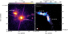 |
Fig. 1 Overview of the HH 48 system. Left: scattered light observations of HH 48 with HST at 0.8 µm on a logarithmic scale to highlight the weak features. The jets observed with HST at 0.6 µm are overlaid in orange, and the ALMA Band 6 continuum (1.3 mm) is overlaid in white. The beam of the ALMA Band 6 observations (0″.10 × 0″.07) is shown in the lower left corner. Right: the integrated CO J = 3−2 emission in HH 48, with Band 7 continuum (0.89 mm) contours overlaid in red. The beams of both observations (0″.51 × 0″.31) are shown in the lower left corner. |
Gas and dust morphologies
The ALMA observations include the NE and SW components of the HH 48 system, which are both detected in CO J = 3−2 and continuum emission. The SW source is considerably brighter than the NE source in both line emission and continuum. HH 48 SW has a diffuse tail of low-intensity CO emission that extends ~4–5″ toward the southwest (see Fig. 1). However, as HH 48 NE is the primary focus of this paper, further exploration of HH 48 SW is left to future work.
HH 48 NE shows a clear disk-like morphology with evidence of possible radial substructure in both continuum and CO line emission. A few suggestive emission minima and maxima are visible in Fig. 1. In the 0.9 and 1.3 mm continuum observations, the disk is resolved along the radial direction with a major axis size of 1.7″ (310 au at the distance of HH 48 NE), but is unresolved along the vertical direction. The beam of the observations is elongated in the North-South direction due to the southern position of HH 48 on the sky. The size of the CO gas disk extends 2.4 times further than the Band 7 continuum, with radii that enclose 95% of the effective flux of 1.7″ and 0.7″, respectively. The CO shows a nonaxisymmetric feature at the western edge of the NE source. At the current resolution of the ALMA observations, it is particularly difficult to discern the origin of this CO feature, which might be the physical disk structure (i.e., a warp), an elevated CO emitting surface (e.g., Law et al. 2021), or dynamical interactions between the outer edges of the NE and SW sources.
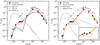 |
Fig. 2 Comparison between the observed and modeled spectral energy distributions of HH 48 NE. Left: observed SED of HH 48 NE (black) and observations for the two components of the binary system combined (gray). The flux values for HH 48 NE are listed in Table 1. The colored lines show the results of the three different MCMC runs described in Sect. 3. The dashed gray line shows the 4155 K stellar input spectrum scaled to a distance of 185 pc. The purple diamonds mark the two points that are scaled from the combined spectrum, as explained in the main text. Right: comparison of the best-fitting model in the SED runs with and without a cavity. |
2.2.3 Spectral energy distribution
The SED was carefully compiled from the literature using observations that resolved the NE and SW components (Fig. 2; Table 1). All observations with a beam larger than twice the distance between the two sources in the binary (i.e., >4.6″) are dominated by the southwest component and should therefore be taken as upper limits. We included observations taken by Gaia, the HST, Spitzer, and ALMA. Unfortunately, the SED has a gap between 24 and 890 µm, where photometry of the combined system was taken at a resolution that was insufficient to separate the binary pair. No observatory is currently able to observe at this wavelength, so we were forced to scale the combined photometry to account for the NE component. In this part of the spectrum, the continuum mainly corresponds to thermal emission from the cold dust in the outer disk. From 890–2800 µm, the flux ratio of the two components remains approximately the same. Therefore, we assumed the same fraction of flux (Fv = HH 48 NE / HH 48 combined) as was measured at 890 µm for the 100 and 300 µm observations and scaled the Herschel intensities by this factor. The addition of these wavelength points, although with intensities including a higher error bar, are essential to discard models with SEDs that significantly deviate in this wavelength range. In Fig. 2 we also show the observed fluxes of the two sources combined, which must not be exceeded by either of the binary components. The uncertainties on all data points were increased to 5% to account for short-term variability that often occurs in young systems like these (Espaillat et al. 2019; Zsidi et al. 2022).
3 Modeling
Our modeling was based on the full anisotropic scattering radiative transfer capabilities of RADMC-3D (Dullemond et al. 2012). The specific steps of our modeling and fitting procedure are described in the following sections.
3.1 Model setup
The model setup we used was fully parameterized, assuming an azimuthally symmetric disk with a power-law density structure and an exponential outer taper (Lynden-Bell & Pringle 1974),
![Mathematical equation: $\sum\nolimits_{{\rm{dust}}} { = {{\sum\nolimits_{\rm{c}} {} } \over }{{\left( {{r \over {{R_{\rm{c}}}}}} \right)}^{ - \gamma }}\exp \,\left[ { - {{\left( {{r \over {{R_{\rm{c}}}}}} \right)}^{2 - \gamma }}} \right]} ,$](/articles/aa/full_html/2023/09/aa46052-23/aa46052-23-eq1.png) (1)
(1)
where Σc is the surface density at the characteristic radius, Rc, γ is the power-law index, and e is the gas-to-dust ratio. The inner radius of the disk was set to the sublimation radius, approximated by  , and the outer radius of the grid was set to 300 au (1.6″). The stellar input spectrum was approximated by a blackbody with temperature (Ts) scaled to the stellar luminosity (Ls).
The height of the disk is described by
 (2)
(2)
where h is the aspect ratio, hc is the aspect ratio at the characteristic radius, and ψ is the flaring index. The dust density has a vertical Gaussian distribution,
![Mathematical equation: ${\rho _{\rm{d}}} = {{\sum\nolimits_{{\rm{dust}}} {} } \over {\sqrt {2\pi } rh}}\exp \,\left[ { - {1 \over 2}{{\left( {{{{\pi \mathord{\left/ {\vphantom {\pi {2 - \theta }}} \right. \kern-\nulldelimiterspace} {2 - \theta }}} \over h}} \right)}^2}} \right],$](/articles/aa/full_html/2023/09/aa46052-23/aa46052-23-eq4.png) (3)
(3)
where θ is the opening angle from the midplane as seen from the central star.
We adopted the canonical gas-to-dust ratio of 100 to scale between the total disk mass and the total mass in dust grains. Dust settling was parameterized by separating the total dust mass over two dust populations: one population of small grains covering the full vertical extent of the disk, and another population with large grains that was limited in height to X • h with X ϵ [0, 1]. The minimum grain size and maximum grain size of the small dust population were allowed to vary to simulate variations in grain growth. The minimum grain size of the large dust population was fixed to the minimum size of the small dust population, and the maximum grain size of the large dust population was fixed to 1 mm. The two dust populations followed a power-law size distribution with a fixed slope of −3.5. The fraction of the total dust mass that resides in the large dust population was defined as fe. We assumed a grain composition consistent with inter stellar matter (ISM) dust, consisting of 85% amorphous pyroxene Mg0.8Fe0.2SiO3, 15% amorphous carbon, and a porosity of 25% (see, e.g., Weingartner & Draine 2001 and Andrews et al. 2011 for an observational justification of these fixed parameters).
The dust and ice opacities were calculated using OpTool (Dominik et al. 2021), using the distribution of hollow spheres (DHS; Min et al. 2005) approach to account for grain shape effects. We used the full anisotropic scattering capabilities of RADMC-3D because isotropic scattering assumptions can have a significant impact on the amount of observed scattered light in the near- to mid-infrared (Pontoppidan et al. 2007).
The ALMA continuum and CO gas observations suggest that the system has an inner cavity, which we discuss in more detail in Sect. 4.5. To account for this in the models, we removed dust and gas inside Rcav by multiplying the surface density by a constant factor δcav, following the approach taken in Madlener et al. (2012), to simulate the removal of gas and dust in the inner disk region.
In total, we have 14 free parameters that were varied to find the best-fitting model for HH 48 NE: two stellar parameters (Ls, Ts), six geometric parameters (Rc, hc, ψ, i, γ, Mgas), four parameters describing the two dust populations (fe, X, amin, amax), and two variables describing the cavity (Rcav and δcav).
SED of HH 48 NE.
3.2 MCMC modeling
To find a model that represents HH 48 NE the best, we applied Markov chain Monte Carlo (MCMC) modeling on resolved observations of the disk in scattered light, the highest S/N ALMA Band 7 millimeter continuum, and the SED. MCMC is a method for sampling from probability distributions with an unknown normalization constant to converge to a global minimum in the difference between a model and observations. Since we explored a highly degenerate multiparameter space, we used a parallel tempered approach (Earl & Deem 2005). In parallel tempered MCMC, multiple runs sample from the probability distribution at the same time, each with a different measure (temperature) of how likely low-probability regions in the probability distribution will be crossed. By occasionally exchanging states between these different runs, the chain of interest is less likely to remain stuck in local minima of the probability space. We used the python MCMC implementation emcee (Foreman-Mackey et al. 2013), using two different likelihood temperatures in the parallel tempered approach.
We used three observables on wich we evaluated our model: a complete SED from 0.5–3000 µm (see Fig. 2), HST scattered light observation at 0.8 µm (see Fig. 1, left panel), and ALMA continuum observation at 890 µm (see Fig. 1, right panel). We only used the ALMA Band 7 continuum data because data set has the highest S/N, but we compare the Band 6 continuum data extensively to the model outcome in Sect. 4.5. Combining the different observables in one evaluation at every step in the Markov process is nontrivial because the sources of uncertainty are different in each step. Weighting the importance of the individual χ2 values is therefore not straightforward. For the easiest understanding of the likelihood of each data set given by our model, we conducted three independent MCMC runs with one of the observables as input. We refer to these MCMC runs as the SED run, the HST run, and the ALMA run. An additional MCMC fit on the SED was performed without a cavity in the model for a comparison with the runs with the cavity, and to gauge how robust the different parameters are. We refer to this run as the SED run without a cavity.
The models were evaluated using a χ2 value,
 (4)
(4)
where N is the number of observables, µi is the modeled observable, Oi is the data points, and  is the corresponding error estimate. The log-likelihood in emcee was set to
 (5)
(5)
For the SED runs, evaluating χ2 is straightforward because we can directly compare the total flux in the model with the observations and their respective uncertainty. The modeled SEDs were corrected for foreground visual extinction. The Av value was treated as an independent parameter that was determined after every run by reducing the  value to a minimum assuming Av ≥ 0 mag. The correction functions were taken from Cardelli et al. (1989) if Av < 3 mag and from McClure (2009) otherwise. For the HST and ALMA runs, we convolved the ray-traced 2D images with a Gaussian beam/point spread function (PSF) similar to that of the observations and rebinned the images to the same resolution as the observations. After this, we used an autocorrelation to find the optimal position of the model. The χ2 value was then determined over the pixels in the region with a 5σ detection in the data (white contours in Fig. 3) to avoid overfitting on noise features. The images were normalized to the peak flux in the observations and models to focus on the spatial distribution without the total flux at only one wavelength in the fit (as opposed to the SED run, which fit the total flux from 0.5–3000 µm).
We let 200 walkers (more than ten times the number of free parameters) explore the parameter space for 500 steps in each of the three different runs, resulting in 2 × 10⁵ models per run. A physically motivated prior was applied to the parameter space, which means that we rejected models that were not feasible given our knowledge of the general population of T Tauri stars to avoid long run-times and to facilitate convergence. The priors were uniform distributions within the ranges given in Table 2. The disk mass, cavity depletion, grain sizes, and settling fraction were sampled logarithmically to support the variations of many orders of magnitude that are physically possible. The starting position of each of the walkers was randomly sampled using a uniform distribution in a region around a selected model that fit the SED reasonably well. The walkers quickly spread out to sample every corner of the parameter space. The first 100 steps were considered the burn-in stage and were not taken into account for the statistics.
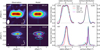 |
Fig. 3 Comparison between the ALMA (890 µm, top) and HST (0.8 µm, bottom) observations with the ray-traced model. Far left: observations of HH 48 NE normalized to the peak emission. The size of the beam/PSF is indicated in the bottom left corner. The white lines trace the 5σ contours of the observations. Center left: best-fitting model at the same wavelengths as the observation, convolved with a model of the beam or PSF. The colored lines trace the same value relative to the peak flux, as the 5σ contour of the observation in the model images for the SED run (red), the HST run (cyan), and the ALMA run (purple). The dashed cyan line illustrates the position of the radial and vertical cuts shown in the right panel. Center right: radial cut through the observations (black) and the three models using the SED (red), the resolved HST observation (cyan), the ALMA observation (purple) (see Sect. 3). The radial cuts are normalized to their respective peak flux. Far right: normalized vertical cut through the data and models as for the radial distribution. The vertical cut through the HST observations is 0.25″ off-center to obtain the highest S/N of the lower lobe. |
4 Results
The results of the individual runs are summarized in Table 2, and the uncertainties are given by the 16th and 84th percentiles. The full posterior distributions can be found in Appendix A. The MCMC runs converge to a very similar model in terms of physical parameters and geometry.
In the next section, we describe the results from the four independent MCMC runs on the SED, the HST observation in scattered light, and the ALMA observation of the warm dust continuum. We selected of the best-fitting representative (all parameters within 1σ) models out of each run for a comparison with the data, and we discuss the import of each of the parameters on the geometry and dust distribution of the HH 48 NE disk. The choice of parameters for the best model in each run is indicated in Fig. A.1 and given in Table 2 with the corresponding χ2 value on each observable. The simulated observations are compared to the data in Figs. 2 and 3. In the ideal case, all MCMC runs would end in the same place in the parameter space, but this is unrealistic because each of the observables is sensitive to a different subset of the free parameters and because the parameterized model does not account for local changes in surface density, settling, or radial drift, for instance. The benefit of having separate runs for the different observables is that we can provide our own weights for the constraints of the different runs. In this particular case, the outcomes of the different MCMC runs are consistent with each other within the error bars for most parameters (see Table 2). The best-fitting model from the SED run was taken as the overall best fit to the data and will be used as a fiducial model in the ice analysis in Paper II. This specific model was chosen as it fits the photometric data points in the mid-infrared (see Fig. 2), which is crucial for modeling the ices in Paper II and for the comparison with JWST data in later papers. It also reproduces the main features of the ALMA and HST observations (see Fig. 3).
4.1 Stellar parameters
The best fit stellar parameters are consistent with the K7 spectral type in the literature for the combined system (Luhman 2007). We find a slightly higher mean stellar effective temperature than the typical temperature of ~4000 K for a K7 star (Pickles 1998), but the uncertainty on the temperature is significant (10–15%) in each of the runs. The luminosity is well constrained at 0.4±0.1 L⊙ but is partly degenerate with the foreground extinction (Av) that could not be constrained from other observations due to the obscuration of the star. The visual extinction from foreground clouds is ~5 in the best-fitting model, which is consistent with Gaia measurements of the extinction toward nearby stars.
To better constrain the stellar parameters of HH 48 NE, we applied dynamical mass fitting to the CO J = 3−2 rotation map. CO rotation maps can be used to derive the dynamical mass of the HH 48 NE disk, assuming that the gas is in Keplerian rotation around the central star. We generated a rotation map of CO J = 3−2 using the quadratic method of bettermoments and excluded regions in which the peak intensities were lower than three times the RMS. Figure 4 shows the resulting map. We then fit this rotation map with eddy (Teague 2019), which uses the emcee (Foreman-Mackey et al. 2013) Python code for MCMC fitting. We used 64 walkers to explore the posterior distributions of the free parameters, which take 500 steps to burn in and an additional 500 steps to sample the posterior distribution function.
We considered only two free parameters for modeling the Keplerian velocity fields: the stellar host mass (M*), and the systemic velocity (vlsr). Due to difficulties in interpreting the source morphology, as noted in Sect. 2.2.2, and the relatively large and asymmetric beam size, we fixed the coordinates of the disk center, which were visually estimated from the CO J = 3−2 map. We adopted the best-fit model inclination value of 82.3°. The estimates of M*, were found to be particularly sensitive to the choice of PA, which is again difficult to constrain due to uncertainties in the gas structure of HH 48 NE and the significant non-Keplerian gas motions, as labeled in Fig. 4. We thus ran fits with a range of plausible PA values between 80 and 95° in increments of 2.5°. We note that when we adopted the PA value of 75° derived from the continuum in Villenave et al. (2020), a nonconverging fit resulted, which again suggests that HH 48 NE likely has a complex gas and dust structure that is only marginally resolved in the current ALMA observations.
Overall, we find best-fit velocity fields consistent with a vlsr of ∼4.4−4.9 km s−1 and a stellar host mass of ∼1−1.4 M⊙. Statistical uncertainties on any individual fit are ∼20−40%, which do not include the systematic uncertainties on each fixed parameter. Figure 4 shows a representative fit to the rotation map. Higher angular resolution observations of gas in the HH 48 system would greatly alleviate these difficulties and allow for a significantly more robust dynamical mass determination.
With the modeled evolutionary tracks, we determined whether the combination of stellar parameters we found was theoretically feasible. Siess et al. (2000) modeled the physical evolution of protostars using the Grenoble stellar evolution code in an extensive grid of initial conditions and listed the main stellar properties as a function of time (mass, luminosity, temperature, etc.). Using their evolutionary tracks for solar metallicity, we find that the luminosity (0.41 L⊙) and temperature (4070 K) of the best-fitting model from the SED run are consistent, within the uncertainty of the MCMC runs, with the dynamical mass. These values agree with the literature K7 spectral type, as we discuss further in Sect. 5.1.
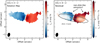 |
Fig. 4 Dynamical mass fitting of HH 48 NE. Left: rotation map of the ALMA CO J = 3−2 observations in HH 48 NE. The spatial offset on the axes is with respect to the telescope pointing (HH 48 SW; RA: 166.0953°, Dec: −77.30207°). The beam size is shown as a black ellipse in the bottom left corner (0″.51 × 0″.31). Right: residuals after subtracting the model from the observations. The gray ellipses indicate the regions we used for the fitting. The innermost two beams were masked to avoid confusion from beam dilution, and the outer radius was visually determined to avoid nondisk-like emission. |
4.2 Spatial disk parameters
The disk in HH 48 NE has a characteristic radius of ∼90 au, with a power-law density index slightly lower than the canonical value of 1. The physical disk size estimate is 30% smaller in the ALMA run than in the SED and HST runs, with a best-fitting  au and γ = 0.5 ± 0.1, compared to
  au and γ = 1.0 ± 0.2 in the HST observation. The disk appears similarly extended in the ALMA continuum image compared to the scattered light observations (see Fig. 1), but with a very steep outer cutoff (∆r/r = 0.4 ± 0.1; Villenave et al. 2020). In the model, we show that the disk might be significantly smaller in the millimeter continuum than in the scattered light observations when radiative transfer and optical depth effects are taken into account. This is consistent with most observations of protoplanetary disks (Villenave et al. 2020), and it may be due to radial drift of the largest dust grains. It might also arise because small dust grains follow the gas interaction between the two components (see Fig. 1).
The disk is moderately thick with an aspect ratio, hc, of 0.2–0.25 and a flaring index, ψ, of 0.15−0.2. These values are constrained the most by the HST run, but agree within the error bars with the SED and ALMA runs. hc and the settling height X are degenerate in the ALMA run because the millimeter continuum wavelengths trace the largest grains that only exist in the large-grain population that is settled with a constant X with respect to the height of the small dust grains and gas. By comparing the outcomes of the SED and HST runs, both of which trace small grains and can therefore constrain the aspect ratio better, we can conclude that the large millimeter-sized grains are settled to 20–25% of the disk scale height. The mass fraction of grains that is settled to the midplane is discussed in Sect. 4.4.
The disk is found to be inclined at 82–84° from the SED and HST runs. The ALMA MCMC run suggests a higher inclination of 88°, but these high inclinations clearly contradict the scattered light observations (see Fig. 3). A similar anomaly has been seen in the extensive modeling of Oph 163131 by Wolff et al. (2021), who reported a similar offset in inclination between the scattered light observations and the ALMA continuum (which was subsequently resolved by observations at a higher angular resolution; Villenave et al. 2022). Because the ALMA image is not resolved in the vertical direction and is only resolved with four to five beams along the radial direction, it is hard to break the degeneracies between the inclination and several other parameters such as hc and Rc (see Appendix A). In the end, we find that an inclination of ~83° is more probable based on the appearance of the disk in scattered light, and this inclination reproduces the ALMA image relatively well (see Fig. 3).
4.3 Mass
The total mass of the disk is determined from the MCMC runs to be 2.5 − 10 × 10−3 M⊙, assuming a gas-to-dust ratio of 100. The disk mass and fraction of large grains are directly proportional with each other in the ALMA run (see Appendix A) because the ALMA observations only trace the large grains. The mass found in the ALMA run is consistent with the SED run within the systematic error when a best-fit value of fe = 0.9 is used. The mass estimate we found based on the HST run is four times higher than the values found in the ALMA and SED runs. High density is needed to explain the broad radial emission seen in scattered light. The SED run fits the west wing of the upper surface in the scattered light image reasonably well (Fig. 3), but fails to fit the asymmetric extension on the east side of the disk. However, the higher total disk mass clearly contradicts the SED (see Fig. 2), which is visible as an underprediction of flux in the near- and mid-infrared and as an excess of flux at millimeter wavelengths. Therefore, the lower mass estimate is more probable.
Using the continuum flux at 0.89 mm (Villenave et al. 2020) and 2.8 mm (Dunham et al. 2016), we compared these values to the lower limit of the total disk mass from the observed millimeter flux using
 (6)
(6)
where d is the distance, Bv(Td) is the Planck function at the isothermal temperature Td, taken as 20 K, κv is the dust opacity at the observed frequency, and the factor 100 is used to convert dust mass into total disk mass. Using our opacities for the large dust grain population, we find an opacity of 9.1 cm2 g−1 and 2.3 cm2 g−1, corresponding to a mass estimate of 1.2 ± 0.1 × 10⁻³ M⊙ and 2.4 ± 0.3 × 10⁻³ M⊙ for the observations at 0.89 mm and 2.8 mm, respectively. The mass estimate at 0.89 mm is significantly lower than the estimate at 2.8 mm, which indicates that the observations at 0.89 mm are still optically thick and that we do not trace the full column of dust. Because the column densities along the line of sight increase with inclination, this is not surprising for a disk this massive (see also the discussion in Villenave et al. 2020). The mass we find in the MCMC runs agrees with these direct estimates when the bulk of the disk is assumed to be optically thin at 2.8 mm.
4.4 Grain properties
The minimum grain size of the small dust distribution is constrained to be 0.2–0.4 µm, excluding nanometer-sized dust grains in the disk atmosphere completely. The maximum grain size of the small dust distribution is constrained to be 8–12 µm. The small grain size distribution is best constrained by the mid-infrared part of the SED (5–100 µm) and the scattered light observations. The posterior distribution in the ALMA run is much broader because the millimeter wavelength radiation is only changed via the disk temperature structure when the grain size distribution is varied, rather than directly via the scattering properties. However, the estimates based on ALMA agree well with the HST and SED runs.
We consistently find that about 90% of the dust mass is settled toward the midplane in large grains at a maximum height of 20–25% of the small grains (see Sect. 4.2 for the discussion of the settling height). Both the SED and the HST observations are extremely sensitive to the amount of settling, resulting in small uncertainties on the number of small grains in the disk atmosphere. At inclinations <85°, the disk needs to be vertically extended and to have a sufficient number of small dust grains in the upper layers of the disk to block direct lines of sight or strong forward scattering from the star. More dust settling hence quickly results in a strong central peak in the synthesized scattered light image. This is not observed in the HST observation (see also Fig. 5 in Paper II).
4.5 Cavity
A cavity must be included in the model to fit all three observables at the same time. To show this, we ran an additional MCMC fit on the SED without a cavity (last column in Table 2), and we show the SED of the resulting best-fit model in Fig. 2.
4.5.1 SED comparison
The modeled SEDs of the runs with and without a cavity look largely the same, but the mid-infrared flux is underestimated in the model without a cavity. The cavity decreases the amount of warm dust in the inner regions of the disk, but photons from the warm inner disk regions can escape much easier because the density is significantly lower. These photons can then again scatter at the surface into our line of sight. Since scattering of dust-emitted photons dominates the observed flux in the mid-infrared (2–15 µm) and this process is more efficient at longer wavelengths, where a larger part of the inner disk is optically thin, the cavity effectively boosts the flux at mid-infrared wavelengths (2–15 µm) compared to optical wavelengths (0.4–0.8 µm). This allows combinations of parameters that fit both the optical wavelengths and the mid-infrared wavelengths in the SED.
The parameters of the SED without a cavity largely agree with the SED run with a cavity (see Table 2), but this run prefers a significantly cooler star (3500 K) with a lower level of visual extinction to compensate for the flux deficit in the mid-infrared. This lower temperature contradicts the measured dynamical mass and is still not able to account fully for the excess flux between 2 and 15 µm (see Fig. 2).
4.5.2 Resolved continuum comparison
Additionally, the steep radial profile with a dip in the continuum detected at 3σ (see Fig. 5) suggests that the inner region of the disk is either depleted in solids or is inclined close to 90° and thus is optically thick (Villenave et al. 2020). Since the latter is excluded by the HST and SED runs, it is likely that these signatures are due to an inner cavity. The model of the SED run without a cavity has a strongly centrally peaked radial profile in ALMA and does not reproduce the 1″ emission plateau and potential dip at the center (see Fig. 5). We would like to note that the effect of the cavity in the HST image is small because of the high optical depth at visible wavelengths.
The ALMA Band 6 (1.3 mm) continuum lacks any obvious cavity, which sets clear limits on the size and depth of the cavity. Our best-fitting model reproduces the size of the radial extent in the ALMA Band 6 continuum, as well as the emission plateau of ∼1″. Models without a cavity and similar inclinations are centrally peaked and do not result in the flat profile that we observed in the ALMA Band 6 and Band 7 continuum. Only very high inclinations would be an option (see the discussion in Villenave et al. 2020), but they are excluded by the SED and scattered light observations. As a next step, an inner disk or a radius-dependent dust depletion factor inside the cavity might be included in order to produce a better combined fit to the Band 6 and Band 7 data. This is beyond the scope of this paper, however.
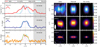 |
Fig. 5 Observed radial profiles of CO and millimeter continuum from ALMA observations compared to models with and without a cavity. Left: radial profile of the CO J = 3−2 integrated emission map (red, top), Band 7 continuum (blue, middle), and Band 6 continuum (orange, bottom). The beam size of the observations in the radial direction is illustrated with a black Gaussian profile in the upper left corner. The modeled emission is shown with a dashed line and is normalized to the peak of the observed profile. The best-fitting or fiducial model is shown in cyan, the best-fitting model without a cavity is shown in purple, a similar model to the best model, but with a cavity that is 100 times more depleted in gas, and dust is shown in gray. The position of HH 48 SW is marked with a gray shaded area. Right: 2D maps of the CO J = 3−2 integrated emission (top), Band 7 continuum (middle), and Band 6 continuum (bottom). Images are rotated by 12 degrees so that the disk is aligned horizontally. From left to right: observations, overall best-fitting model, and best-fitting model without a cavity. The beam sizes of the observations are shown in the lower left corner. |
4.5.3 Comparison of the gas observation
Last, the CO J = 3−2 line emission reveals a 50% dip at a position similar to that seen in the dust continuum (see Fig. 5), and this can only be reproduced when a cavity is included or when the foreground cloud contributes significantly to the observations. Since the foreground visual extinction is low (Av ∼ 5 mag) and a similar dip is not observed toward HH 48 SW, the latter is unlikely. To estimate the depth of the cavity in the gas, we added CO gas to the model at a number abundance of 10−4 with respect to H nuclei. To mimic freeze-out, we removed all CO gas from disk regions that were colder than 20 K, the typical desorption temperature of CO. Photodissociation was approximated by removing all CO at gas densities lower than 107 cm−3. The CO level populations were determined in RADMC–3D using anonlocal thermal equilibrium large velocity gradient approach assuming that the gas temperature is the same as the dust temperature. The CO J = 3−2 line was then ray-traced at a velocity resolution of 0.5 km s−1. This simple approach is not meant to build the perfect gas model of HH 48 NE because it has severe limitations and crude approximations, but should only be considered as a quick comparison.
We show the integrated emission of the modeled CO J = 3−2 line with its radial profile in Fig. 5. The radial profile of the best-fitting model has a clear dip at the center, similar to the observations. The dip is not as deep as in the observations, which could be due to the fact that we assumed the gas temperature to be the same as the dust temperature, which is no longer true in a cavity (Bruderer 2013; Leemker et al. 2022). Decreasing the amount of material in the cavity by two additional orders of magnitude does reproduce the depth of the gas cavity (gray line in Fig. 5), but is a poorer fit to the continuum and has a significant impact on the SED. The best-fitting model without a cavity does not reproduce the observed radial profile and is strongly centrally peaked. Hence, the gas observations show additional evidence that the disk likely is depleted in dust and gas in a central region of the disk. The modeled emission agrees with the observations in the inner 1″, but fails to reproduce the wings that extend beyond the size of the disk in millimeter emission. The gas in the disk extends farther out than the dust, which is likely a result of radial drift (see, e.g., Andrews et al. 2011; Trapman et al. 2019).
4.5.4 Size and depth
The cavity is constrained to be 50–70 au, where dust is depleted by two orders of magnitude. An empty cavity results in an underestimation of the mid-infrared part of the SED, so some warm dust must be available in the inner cavity. However, it is impossible to distinguish between a depleted but not empty cavity and a fully depleted cavity with a small inner disk with sufficiently warm dust. The cavity appears larger in the millimeter observations ( ) than in the SED and HST observations (∼50 au), which may be partly attributed to the poor spatial resolution of the latter observations. However, this may also be partly due to radial dust segregation if the small dust grains follow the gas further into the cavity than the large dust grains. Similar dissimilarities between the scattered light observations and millimeter continuum are seen in almost all transition disks (Villenave et al. 2019; Sturm et al. 2023a; van der Marel 2023; Benisty et al. 2022).
5 Discussion
The source structure of HH 48 NE is in many ways in line with our current understanding of protoplanetary disk physics. The height, mass, and radial extent of the disk suggest that HH 48 NE has a typical T Tauri disk that would not stand out of the population of observed protoplanetary disks at lower inclination (see, e.g., Ansdell et al. 2016; Manara et al. 2023). Cavities are relatively common in class II disks (see, e.g., van der Marel & Mulders 2021). The two main differences between this disk and the average disk are its relatively low-mass fraction of settled large dust grains and high inclination. Previous infrared surveys of disks in Chamaeleon I reported that between 99 and 99.9% of the dust mass in the upper layers of the disk had settled to the midplane (Manoj et al. 2011), consistent with disks in other 1–3 Myr old molecular clouds such as Taurus and rho Ophiuchus (Furlan et al. 2011; McClure et al. 2010). In contrast, only 90% of the dust has settled in the disk around HH 48 NE. Based on the paucity of bona fide edge-on disk detections, we speculate that the known edge-on disks might be detectable because they possess the combination of (at most) moderate dust settling and high inclination. We address this question in Paper II and discuss the implications of our concordant best-fitting model for the disk physical properties below (see also the recent paper by Angelo et al. 2023).
5.1 Convergence of fit
Multiwavelength dust fitting including the SED and resolved observations often leads to discrepancies in which the scattered light observations push the model geometry in a different direction than either the continuum observations or the SED, for example (see, e.g., Wolff et al. 2017, 2021). Therefore, more complicated attempts such as using a staggered Markov chain (Madlener et al. 2012) or covariance matrices (Wolff et al. 2017) are explored in the literature, each with their promises and limitations. We have shown that three separate MCMC runs on the SED, scattered light HST observations, and millimeter-continuum ALMA observations converge to a model that reproduces these three observables to a reasonable extent. Additionally, we show in Fig. 6 that the temperature and luminosity in the best-fitting model are in line with the measured dynamical mass of the system, and the age spread in the Chamaeleon I star-forming region (4–5 Myr is on the old end of the age spread in the Chamaeleon I star-forming region; Galli et al. 2021). For this reason, we kept the procedure as simple as possible, without combining the different observations. As we have shown in Sect. 4, individual differences between the outputs of the runs can provide insight into the effects of dust dynamics on differently sized grains. In principle, radial segregation of grain sizes and/or radial drift in the model could be accounted for, but this would introduce additional free parameters and would complicate the MCMC fits while the data may not have high enough S/N and/or spatial resolution to definitively draw conclusions on the differences between large and small grains.
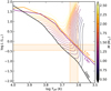 |
Fig. 6 Hertzsprung-Russel diagram with stellar tracks from Siess et al. (2000) for stellar masses from 0.5 to 2.5 M⊙. The orange and purple lines denote the 4 and 5 Myr isochrones. The crosshair points at the range of effective temperature and luminosity found in the MCMC runs, which agrees well with a ∼1 M⊙ star derived from the dynamical fits to the CO emission. |
5.2 Grain size distribution
The dust grains in the atmospheric layers of the disk in HH 48 NE are constrained to have a size between 0.3 and 10 µm. The minimum grain size found in the disk is much larger than in the ISM dust distribution (typically 0.005 µm). This result is consistent with previous findings of Pontoppidan et al. (2007), showing that the high mid-infrared scattered light continuum in the Flying Saucer can only be explained by a dust distribution in the disk atmosphere with large grains (0.25−16 µm). Our result is also consistent with previous simple comparisons of opacities with single-grain sizes to Spitzer/IRS observations of the silicate feature at 10 µm. Olofsson et al. (2009) find that the observed silicate features in a large (96) sample of T Tauri disks are mainly produced by micrometer-sized grains. They show that there cannot be a large number of submicrometer-sized dust grains in the disk atmosphere because their emission would overwhelm the few large grains. Additionally, Tazaki et al. (2021) reported evidence for grains greater than micrometers in the upper layers of the HD 142527 disk with an independent method, using resolved H2O ice observations in coronagraphic imaging of scattered light (see also Honda et al. 2009). The grain size limits are on the high end compared to the range found using the SEDs of 30 well-known (low-inclination) protoplanetary disks (Kaeufer et al. 2023). Kaeufer et al. (2023) used a Bayesian analysis to determine accurate parameter values with their uncertainties, and found a minimum grain size of typically 0.01–0.2 µm and a maximum grain size of typically 1–9 µm.
Grains larger than 1 µm are thought to settle quickly to the midplane (<105 yr; Dullemond & Dominik 2004) in the relevant regions (<100 au) because of the frictional force between the Keplerian orbit of the grain and the slightly sub-Keplerian orbit of the gas because of the pressure support. Together with the very low levels of turbulence in lower disk regions (e.g., Pinte et al. 2016; Villenave et al. 2022; Flaherty et al. 2020, and the references therein), this means that some mechanism has to segregate dust vertically and prevent the micrometer-sized dust grains from settling to the midplane or replenishes the micrometer-sized dust grains via grain-grain fragmentation, but does not affect the millimeter-sized dust grains observed with ALMA. Some theoretical sources of turbulence can cause efficient vertical mixing, but do not reach all the way to the midplane (zombie vortex instability; Barranco et al. 2018; see also Lesur et al. 2022). This particular source of turbulence is likely available in the strongly stratified regions of all protoplanetary disks as long as there is modest grain settling and/or growth (Barranco et al. 2018; Lesur et al. 2022). Only non-physically fast cooling and a high viscosity are known to suppress the instability (Lesur & Latter 2016). Mechanisms such as these are a promising solution to the micrometer-sized dust grains in the upper layers of the disk, but need to be studied further in simulations to determine whether any direct observational signatures can serve as proof of their existence.
In addition, there has to be a mechanism that efficiently removes submicrometer grains from the disk atmosphere, but leaves approximately micrometer sized dust grains in the upper disk. This could be possible if growth timescales for these small grains are significantly shorter than the fragmentation timescales (see, e.g., Birnstiel et al. 2011; Windmark et al. 2012). This would require low levels of turbulence, or porous fluffy grains that easily stick together to form larger grains (Birnstiel et al. 2011). Because no ice is available in the disk atmospheres to make the grains stickier due to the extreme temperatures and UV irradiation, this would require that the products of grain-grain fragmentation are inherently porous and fluffy. An additional hypothesis is that the smallest dust grains can be lifted from the surface by disk winds, while the larger grains are too heavy to be carried away (Olofsson et al. 2009; Booth & Clarke 2021). Disk winds might be a ubiquitous driving mechanism for accretion in T Tauri protoplanetary disks (see, e.g., Tabone et al. 2022) and may be launched from a substantial fraction of the disk surface (Tabone et al. 2020). Dust lifting by the wind is only efficient for smaller dust grains (<1 µm) and might significantly deplete the small-dust population if it is sustained for timescales of millions of years (Booth & Clarke 2021). Understanding the vertical dust segregation could be a key element in understanding the origin of turbulence in protoplanetary disks and the weight-lifting capabilities of disk winds.
The exclusion of small nanometer-sized grains from the upper atmosphere of the disk has strong implications for the disk chemistry. In many chemical disk models, the minimum grain size distribution is taken to be the same as for ISM grains (~5 nm; e.g., Bruderer et al. 2012; Walsh et al. 2015). When the average surface area of dust grains in the disk atmosphere were decreased, a higher degree of UV radiation in the deeper disk layers would result. An excess of UV radiation enhances photodissociation and photodesorption processes that ultimately result in a very rich chemistry (Bergner et al. 2019, 2021; Calahan et al. 2023).
5.3 Inner cavity
We have shown that HH 48 NE likely has an inner cavity in the disk in both gas and dust of ~50 au. Similar cavities are found in a relatively large number of face-on disks (transition disks; ~10%; Ercolano & Pascucci 2017), but have not been directly observed in edge-on protoplanetary disks so far. The radial structure of some of the disks in the large sample of Villenave et al. (2020) suggests that radial substructure is present in edge-on disks. However, detailed multiwavelength modeling is necessary to exclude increased dust opacity due to high inclinations in combination with a high disk mass as an alternative explanation for disks with a flat radial flux distribution or central dip. The inclusion of a cavity in our model is crucial to fit the SED in the mid-infrared. The cavity allows photons emitted by warm dust in the innermost region of the disk to escape if they have an ideal angle to scatter along our line of sight. Similar conclusions are drawn from optical and near-infrared observations (see Benisty et al. 2022, for a review) and also lead to a distinction of Herbig Ae/Be stars into group I and group II sources. Group I includes the sources with high levels of optical scattering due to large inner cavities, and group II includes the sources without a cavity and much lower levels of scattering.
Without a cavity, we would need to add a 1400 K black-body to the source spectrum in a similar way as Pontoppidan et al. (2007) to mimic the increasing amount of photons originating from the inner disk regions. Adding a 1400 K blackbody manually solves the discrepancy in the SED fit but is not self-consistent because the 1400 K emission is thought to arise from the inner disk, not from the central star. The difference in solid angle between a stellar point source with an additional 1400 K component and warm inner disk could result in crucial differences when ice features in the mid-infrared are to be modeled because the mid-infrared continuum would be dominated by photons that scatter off of the disk that are produced in the warm inner disk, not in the star itself (see Appendix A in Paper II). We showed that our model is self-consistent and naturally reproduces the flux in the mid-infrared.
Additional research, preferably with higher angular resolution ALMA data, is necessary to determine whether the unnoticed existence of a cavity can resolve this issue in more sources. In edge-on disks, many of the smaller cavities or rings will be hidden behind the optically thick dust in the midplane, and a multiwavelength analysis is necessary to constrain it. In the specific case of the Flying Saucer, where a similar deficit in mid-infrared flux is found as in our model without a cavity (Pontoppidan et al. 2007), the continuum indicates a double-peaked continuum in the radial direction (Guilloteau et al. 2016), even though the dip is weaker and less well resolved than in HH 48. Additional detailed multiwavelength studies of other edge-on disks are necessary to determine whether more of them harbor a cavity.
6 Conclusions
We have developed a disk model using the radiative transfer code RADMC-3D, which includes anisotropic scattering. We ran MCMC fits to HST observations, ALMA observations, and the SED for HH 48 NE to constrain the geometry and physical features of this edge-on class II system. We can conclude the following:
The best-fitting model (SED run) reproduces both the spatially resolved features of the emission in scattered light observations, millimeter dust continuum observations, CO gas observations, and the SED.
HH 48 NE is a K7 star with a mass of 1–1.4 M⊙, an effective temperature of ~4150 K, and a luminosity of ~0.4 L⊙. These values agree with the estimated age of the Chamaeleon I star-forming region following evolutionary stellar tracks from the literature.
HH 48 NE is a typical T Tauri disk in many ways, but stands out due to the lack of small (<0.3 µm) grains in the disk atmosphere. Mechanisms that remove the small dust grains can be the result of efficient sticking of the smallest grains, or of lifting in large-scale disk winds. The exclusion of small grains may have a major impact on the chemistry in the disk because UV radiation can likely penetrate much deeper into the disk because the average surface area of the grains is smaller.
The disk in HH 48 NE likely has a ∼50 au inner cavity in gas and dust that is mostly invisible due to optically thick dust. The cavity boosts the mid-infrared emission in the SED and allows for a unique model that is consistent with the scattered light observations and the millimeter continuum observations at the same time.
Understanding the mechanisms that set grain size distributions and physical properties of protoplanetary disks is crucial. Edge-on disks can be a unique tool for constraining some parameters that are hard to constrain in less strongly inclined disks, such as dust settling and the grain size distribution.
Acknowledgements
We would like to thank the anonymous referee for suggestions that improved the manuscript. We also thank Ewine van Dishoeck for useful discussions and constructive comments on the manuscript. Astrochemistry in Leiden is supported by the Netherlands Research School for Astronomy (NOVA), by funding from the European Research Council (ERC) under the European Union’s Horizon 2020 research and innovation programme (grant agreement No. 101019751 MOLDISK). M.K.M. acknowledges financial support from the Dutch Research Council (NWO; grant VI.Veni.192.241). D.H. is supported by Center for Informatics and Computation in Astronomy (CICA) grant and grant number 110J0353I9 from the Ministry of Education of Taiwan. D.H. acknowledges support from the National Technology and Science Council of Taiwan through grant number 111B3005191. M.N.D. acknowledges the Swiss National Science Foundation (SNSF) Ambizione grant no. 180079, the Center for Space and Habitability (CSH) Fellowship, and the IAU Gruber Foundation Fellowship. This paper makes use of the following ALMA data: ADS/JAO.ALMA#2016.1.00460.S, ADS/JAO.ALMA#2019.1.01792.S. ALMA is a partnership of ESO (representing its member states), NSF (USA) and NINS (Japan), together with NRC (Canada), MOST and ASIAA (Taiwan), and KASI (Republic of Korea), in cooperation with the Republic of Chile. The Joint ALMA Observatory is operated by ESO, AUI/NRAO and NAOJ. The National Radio Astronomy Observatory is a facility of the National Science Foundation operated under cooperative agreement by Associated Universities, Inc. This work makes use of the following software: numpy (van der Walt et al. 2011), matplotlib (Hunter 2007), astropy (Astropy Collaboration 2013, 2018), bettermoments (Teague & Foreman-Mackey 2018), CASA (McMullin et al. 2007), eddy (Teague 2019), emcee (Foreman-Mackey et al. 2013), OpTool (Dominik et al. 2021), RADMC-3D (Dullemond et al. 2012).
Appendix A Posterior distribution continuum fits
In Figure A.1 we present the posterior distribution of the three independent runs using the SED, the resolved scattered light observation, and the resolved millimeter continuum observations. In Figure A.2 we present the posterior distribution of the SED run without a cavity, the physical parameters of which overall agree well with the SED run with a cavity.
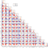 |
Fig. A.1 Posterior distributions of the three different MCMC runs. The SED run is shown in red, the HST run is plotted in orange, and the ALMA run is shown in blue. The median value for each parameter and the 16% and 84% confidence intervals are given in Table 2. |
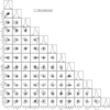 |
Fig. A.2 Posterior distribution of the SED run without a cavity. The median value for each parameter and the 16% and 84% confidence intervals are given in Table 2. |
References
- Andrews, S. M., Wilner, D. J., Espaillat, C., et al. 2011, ApJ, 732, 42 [Google Scholar]
- Angelo, I., Duchêne, G., Stapelfeldt, K., et al. 2023, ApJ, 945, 130 [NASA ADS] [CrossRef] [Google Scholar]
- Ansdell, M., Williams, J. P., van der Marel, N., et al. 2016, ApJ, 828, 46 [Google Scholar]
- Astropy Collaboration (Robitaille, T. P., et al.) 2013, A&A, 558, A33 [NASA ADS] [CrossRef] [EDP Sciences] [Google Scholar]
- Astropy Collaboration (Price-Whelan, A. M., et al.) 2018, AJ, 156, 123 [Google Scholar]
- Barranco, J. A., Pei, S., & Marcus, P. S. 2018, ApJ, 869, 127 [NASA ADS] [CrossRef] [Google Scholar]
- Benisty, M., Dominik, C., Follette, K., et al. 2022, ArXiv e-prints [arXiv:2203.09991] [Google Scholar]
- Bergner, J. B., Öberg, K. I., Bergin, E. A., et al. 2019, ApJ, 876, 25 [Google Scholar]
- Bergner, J. B., Öberg, K. I., Guzmán, V. V., et al. 2021, ApJS, 257, 11 [NASA ADS] [CrossRef] [Google Scholar]
- Birnstiel, T., Ormel, C. W., & Dullemond, C. P. 2011, A&A, 525, A11 [NASA ADS] [CrossRef] [EDP Sciences] [Google Scholar]
- Booth, R. A., & Clarke, C. J. 2021, MNRAS, 502, 1569 [NASA ADS] [CrossRef] [Google Scholar]
- Bruderer, S. 2013, A&A, 559, A46 [NASA ADS] [CrossRef] [EDP Sciences] [Google Scholar]
- Bruderer, S., van Dishoeck, E. F., Doty, S. D., & Herczeg, G. J. 2012, A&A, 541, A91 [NASA ADS] [CrossRef] [EDP Sciences] [Google Scholar]
- Calahan, J. K., Bergin, E. A., Bosman, A. D., et al. 2023, Nat. Astron., 7, 49 [Google Scholar]
- Cardelli, J. A., Clayton, G. C., & Mathis, J. S. 1989, ApJ, 345, 245 [Google Scholar]
- Dominik, C., Min, M., & Tazaki, R. 2021, Astrophysics Source Code Library [record ascl:2104.010] [Google Scholar]
- Dullemond, C. P., & Dominik, C. 2004, A&A, 421, 1075 [NASA ADS] [CrossRef] [EDP Sciences] [Google Scholar]
- Dullemond, C. P., Juhasz, A., Pohl, A., et al. 2012, Astrophysics Source Code Library [record ascl:1202.015] [Google Scholar]
- Dunham, M. M., Offner, S. S. R., Pineda, J. E., et al. 2016, ApJ, 823, 160 [NASA ADS] [CrossRef] [Google Scholar]
- Dutrey, A., Guilloteau, S., Piétu, V., et al. 2017, A&A, 607, A130 [CrossRef] [EDP Sciences] [Google Scholar]
- Earl, D. J., & Deem, M. W. 2005, Phys. Chem. Chem. Phys., 7, 3910 [CrossRef] [Google Scholar]
- Ercolano, B., & Pascucci, I. 2017, Roy. Soc. Open Sci., 4, 170114 [Google Scholar]
- Espaillat, C. C., Macías, E., Hernández, J., & Robinson, C. 2019, ApJ, 877, L34 [NASA ADS] [CrossRef] [Google Scholar]
- Flaherty, K., Hughes, A. M., Simon, J. B., et al. 2020, ApJ, 895, 109 [NASA ADS] [CrossRef] [Google Scholar]
- Flores, C., Duchêne, G., Wolff, S., et al. 2021, AJ, 161, 239 [NASA ADS] [CrossRef] [Google Scholar]
- Foreman-Mackey, D., Hogg, D. W., Lang, D., & Goodman, J. 2013, PASP, 125, 306 [Google Scholar]
- Furlan, E., Luhman, K. L., Espaillat, C., et al. 2011, ApJS, 195, 3 [Google Scholar]
- Gaia Collaboration (Prusti, T., et al.) 2016, A&A, 595, A1 [NASA ADS] [CrossRef] [EDP Sciences] [Google Scholar]
- Gaia Collaboration (Brown, A. G. A., et al.) 2021, A&A, 649, A1 [NASA ADS] [CrossRef] [EDP Sciences] [Google Scholar]
- Galli, P. A. B., Bouy, H., Olivares, J., et al. 2021, A&A, 646, A46 [NASA ADS] [CrossRef] [EDP Sciences] [Google Scholar]
- Guilloteau, S., Piétu, V., Chapillon, E., et al. 2016, A&A, 586, L1 [NASA ADS] [CrossRef] [EDP Sciences] [Google Scholar]
- Honda, M., Inoue, A. K., Fukagawa, M., et al. 2009, ApJ, 690, L110 [Google Scholar]
- Hunter, J. D. 2007, Comput. Sci. Eng., 9, 90 [NASA ADS] [CrossRef] [Google Scholar]
- Kaeufer, T., Woitke, P., Min, M., Kamp, I., & Pinte, C. 2023, A&A, 672, A30 [NASA ADS] [CrossRef] [EDP Sciences] [Google Scholar]
- Law, C. J., Teague, R., Loomis, R. A., et al. 2021, ApJS, 257, 4 [NASA ADS] [CrossRef] [Google Scholar]
- Leemker, M., Booth, A. S., van Dishoeck, E. F., et al. 2022, A&A, 663, A23 [NASA ADS] [CrossRef] [EDP Sciences] [Google Scholar]
- Lesur, G. R. J., & Latter, H. 2016, MNRAS, 462, 4549 [NASA ADS] [CrossRef] [Google Scholar]
- Lesur, G., Ercolano, B., Flock, M., et al. 2022, ArXiv e-prints [arXiv:2203.09821] [Google Scholar]
- Luhman, K. L. 2007, ApJS, 173, 104 [Google Scholar]
- Lynden-Bell, D., & Pringle, J. E. 1974, MNRAS, 168, 603 [Google Scholar]
- Madlener, D., Wolf, S., Dutrey, A., & Guilloteau, S. 2012, A&A, 543, A81 [NASA ADS] [CrossRef] [EDP Sciences] [Google Scholar]
- Manara, C. F., Ansdell, M., Rosotti, G. P., et al. 2023, ASP Conf. Ser., 534, 539 [NASA ADS] [Google Scholar]
- Manoj, P., Kim, K. H., Furlan, E., et al. 2011, ApJS, 193, 11 [NASA ADS] [CrossRef] [Google Scholar]
- Marton, G., Calzoletti, L., Perez Garcia, A. M., et al. 2017, ArXiv e-prints [arXiv:1705.05693] [Google Scholar]
- McClure, M. 2009, ApJ, 693, L81 [NASA ADS] [CrossRef] [Google Scholar]
- McClure, M. K., Furlan, E., Manoj, P., et al. 2010, ApJS, 188, 75 [NASA ADS] [CrossRef] [Google Scholar]
- McMullin, J. P., Waters, B., Schiebel, D., Young, W., & Golap, K. 2007, ASP Conf. Ser., 376, 127 [Google Scholar]
- Min, M., Hovenier, J. W., & de Koter, A. 2005, A&A, 432, 909 [NASA ADS] [CrossRef] [EDP Sciences] [Google Scholar]
- Olofsson, J., Augereau, J. C., van Dishoeck, E. F., et al. 2009, A&A, 507, 327 [NASA ADS] [CrossRef] [EDP Sciences] [Google Scholar]
- Padgett, D. L., Brandner, W., Stapelfeldt, K. R., et al. 1999, AJ, 117, 1490 [CrossRef] [Google Scholar]
- Pickles, A. J. 1998, PASP, 110, 863 [NASA ADS] [CrossRef] [Google Scholar]
- Pinte, C., Dent, W. R. F., Ménard, F., et al. 2016, ApJ, 816, 25 [Google Scholar]
- Podio, L., Garufi, A., Codella, C., et al. 2020, A&A, 642, L7 [NASA ADS] [CrossRef] [EDP Sciences] [Google Scholar]
- Pontoppidan, K. M., Dullemond, C. P., van Dishoeck, E. F., et al. 2005, ApJ, 622, 463 [NASA ADS] [CrossRef] [Google Scholar]
- Pontoppidan, K. M., Stapelfeldt, K. R., Blake, G. A., van Dishoeck, E. F., & Dullemond, C. P. 2007, ApJ, 658, L111 [CrossRef] [Google Scholar]
- Robberto, M., Spina, L., Da Rio, N., et al. 2012, AJ, 144, 83 [NASA ADS] [CrossRef] [Google Scholar]
- Sauter, J., Wolf, S., Launhardt, R., et al. 2009, A&A, 505, 1167 [NASA ADS] [CrossRef] [EDP Sciences] [Google Scholar]
- Siess, L., Dufour, E., & Forestini, M. 2000, A&A, 358, 593 [Google Scholar]
- Stapelfeldt, K. R., Duchêne, G., Perrin, M., et al. 2014, IAU Symp., 299, 99 [NASA ADS] [Google Scholar]
- Sturm, J. A., Booth, A. S., McClure, M. K., Leemker, M., & van Dishoeck, E. F. 2023a, A&A, 670, A12 [NASA ADS] [CrossRef] [EDP Sciences] [Google Scholar]
- Sturm, J. A., McClure, M. K., Bergner, J. B., et al. 2023b, A&A, 677, A18 (Paper II) [NASA ADS] [CrossRef] [EDP Sciences] [Google Scholar]
- Tabone, B., Cabrit, S., Pineau des Forêts, G., et al. 2020, A&A, 640, A82 [CrossRef] [EDP Sciences] [Google Scholar]
- Tabone, B., Rosotti, G. P., Lodato, G., et al. 2022, MNRAS, 512, L74 [NASA ADS] [CrossRef] [Google Scholar]
- Tazaki, R., Murakawa, K., Muto, T., Honda, M., & Inoue, A. K. 2021, ApJ, 921, 173 [NASA ADS] [CrossRef] [Google Scholar]
- Teague, R. 2019, J. Open Source Softw., 4, 1220 [Google Scholar]
- Teague, R., & Foreman-Mackey, D. 2018, Res. notes Am. Astron. Soc., 2, 173 [Google Scholar]
- Teague, R., Jankovic, M. R., Haworth, T. J., Qi, C., & Ilee, J. D. 2020, MNRAS, 495, 451 [NASA ADS] [CrossRef] [Google Scholar]
- Trapman, L., Facchini, S., Hogerheijde, M. R., van Dishoeck, E. F., & Bruderer, S. 2019, A&A, 629, A79 [NASA ADS] [CrossRef] [EDP Sciences] [Google Scholar]
- van der Marel, N. 2023, Eur. Phys. J. Plus, 138, 225 [NASA ADS] [CrossRef] [Google Scholar]
- van der Marel, N., & Mulders, G. D. 2021, AJ, 162, 28 [NASA ADS] [CrossRef] [Google Scholar]
- van der Walt, S., Colbert, S. C., & Varoquaux, G. 2011, Comput. Sci. Eng., 13, 22 [Google Scholar]
- Villenave, M., Benisty, M., Dent, W. R. F., et al. 2019, A&A, 624, A7 [NASA ADS] [CrossRef] [EDP Sciences] [Google Scholar]
- Villenave, M., Ménard, F., Dent, W. R. F., et al. 2020, A&A, 642, A164 [EDP Sciences] [Google Scholar]
- Villenave, M., Stapelfeldt, K. R., Duchêne, G., et al. 2022, ApJ, 930, 11 [NASA ADS] [CrossRef] [Google Scholar]
- Walsh, C., Nomura, H., & van Dishoeck, E. 2015, A&A, 582, A88 [NASA ADS] [CrossRef] [EDP Sciences] [Google Scholar]
- Weingartner, J. C., & Draine, B. T. 2001, ApJ, 548, 296 [Google Scholar]
- Windmark, F., Birnstiel, T., Güttler, C., et al. 2012, A&A, 540, A73 [NASA ADS] [CrossRef] [EDP Sciences] [Google Scholar]
- Winston, E., Cox, N. L. J., Prusti, T., et al. 2012, A&A, 545, A145 [NASA ADS] [CrossRef] [EDP Sciences] [Google Scholar]
- Wolff, S. G., Perrin, M. D., Stapelfeldt, K., et al. 2017, ApJ, 851, 56 [NASA ADS] [CrossRef] [Google Scholar]
- Wolff, S. G., Duchêne, G., Stapelfeldt, K. R., et al. 2021, AJ, 161, 238 [NASA ADS] [CrossRef] [Google Scholar]
- Zsidi, G., Manara, C. F., Kóspál, Á., et al. 2022, A&A, 660, A108 [NASA ADS] [CrossRef] [EDP Sciences] [Google Scholar]
All Tables
All Figures
|
Fig. 1 Overview of the HH 48 system. Left: scattered light observations of HH 48 with HST at 0.8 µm on a logarithmic scale to highlight the weak features. The jets observed with HST at 0.6 µm are overlaid in orange, and the ALMA Band 6 continuum (1.3 mm) is overlaid in white. The beam of the ALMA Band 6 observations (0″.10 × 0″.07) is shown in the lower left corner. Right: the integrated CO J = 3−2 emission in HH 48, with Band 7 continuum (0.89 mm) contours overlaid in red. The beams of both observations (0″.51 × 0″.31) are shown in the lower left corner. |
| In the text | |
|
Fig. 2 Comparison between the observed and modeled spectral energy distributions of HH 48 NE. Left: observed SED of HH 48 NE (black) and observations for the two components of the binary system combined (gray). The flux values for HH 48 NE are listed in Table 1. The colored lines show the results of the three different MCMC runs described in Sect. 3. The dashed gray line shows the 4155 K stellar input spectrum scaled to a distance of 185 pc. The purple diamonds mark the two points that are scaled from the combined spectrum, as explained in the main text. Right: comparison of the best-fitting model in the SED runs with and without a cavity. |
| In the text | |
|
Fig. 3 Comparison between the ALMA (890 µm, top) and HST (0.8 µm, bottom) observations with the ray-traced model. Far left: observations of HH 48 NE normalized to the peak emission. The size of the beam/PSF is indicated in the bottom left corner. The white lines trace the 5σ contours of the observations. Center left: best-fitting model at the same wavelengths as the observation, convolved with a model of the beam or PSF. The colored lines trace the same value relative to the peak flux, as the 5σ contour of the observation in the model images for the SED run (red), the HST run (cyan), and the ALMA run (purple). The dashed cyan line illustrates the position of the radial and vertical cuts shown in the right panel. Center right: radial cut through the observations (black) and the three models using the SED (red), the resolved HST observation (cyan), the ALMA observation (purple) (see Sect. 3). The radial cuts are normalized to their respective peak flux. Far right: normalized vertical cut through the data and models as for the radial distribution. The vertical cut through the HST observations is 0.25″ off-center to obtain the highest S/N of the lower lobe. |
| In the text | |
|
Fig. 4 Dynamical mass fitting of HH 48 NE. Left: rotation map of the ALMA CO J = 3−2 observations in HH 48 NE. The spatial offset on the axes is with respect to the telescope pointing (HH 48 SW; RA: 166.0953°, Dec: −77.30207°). The beam size is shown as a black ellipse in the bottom left corner (0″.51 × 0″.31). Right: residuals after subtracting the model from the observations. The gray ellipses indicate the regions we used for the fitting. The innermost two beams were masked to avoid confusion from beam dilution, and the outer radius was visually determined to avoid nondisk-like emission. |
| In the text | |
|
Fig. 5 Observed radial profiles of CO and millimeter continuum from ALMA observations compared to models with and without a cavity. Left: radial profile of the CO J = 3−2 integrated emission map (red, top), Band 7 continuum (blue, middle), and Band 6 continuum (orange, bottom). The beam size of the observations in the radial direction is illustrated with a black Gaussian profile in the upper left corner. The modeled emission is shown with a dashed line and is normalized to the peak of the observed profile. The best-fitting or fiducial model is shown in cyan, the best-fitting model without a cavity is shown in purple, a similar model to the best model, but with a cavity that is 100 times more depleted in gas, and dust is shown in gray. The position of HH 48 SW is marked with a gray shaded area. Right: 2D maps of the CO J = 3−2 integrated emission (top), Band 7 continuum (middle), and Band 6 continuum (bottom). Images are rotated by 12 degrees so that the disk is aligned horizontally. From left to right: observations, overall best-fitting model, and best-fitting model without a cavity. The beam sizes of the observations are shown in the lower left corner. |
| In the text | |
|
Fig. 6 Hertzsprung-Russel diagram with stellar tracks from Siess et al. (2000) for stellar masses from 0.5 to 2.5 M⊙. The orange and purple lines denote the 4 and 5 Myr isochrones. The crosshair points at the range of effective temperature and luminosity found in the MCMC runs, which agrees well with a ∼1 M⊙ star derived from the dynamical fits to the CO emission. |
| In the text | |
|
Fig. A.1 Posterior distributions of the three different MCMC runs. The SED run is shown in red, the HST run is plotted in orange, and the ALMA run is shown in blue. The median value for each parameter and the 16% and 84% confidence intervals are given in Table 2. |
| In the text | |
|
Fig. A.2 Posterior distribution of the SED run without a cavity. The median value for each parameter and the 16% and 84% confidence intervals are given in Table 2. |
| In the text | |
Current usage metrics show cumulative count of Article Views (full-text article views including HTML views, PDF and ePub downloads, according to the available data) and Abstracts Views on Vision4Press platform.
Data correspond to usage on the plateform after 2015. The current usage metrics is available 48-96 hours after online publication and is updated daily on week days.
Initial download of the metrics may take a while.