| Issue |
A&A
Volume 692, December 2024
|
|
|---|---|---|
| Article Number | A111 | |
| Number of page(s) | 11 | |
| Section | Interstellar and circumstellar matter | |
| DOI | https://doi.org/10.1051/0004-6361/202451475 | |
| Published online | 04 December 2024 | |
The grazing-angle icy protoplanetary disk PDS 453
1
Univ. Grenoble Alpes, CNRS, IPAG,
38000
Grenoble,
France
2
Astronomy Department, University of California Berkeley,
Berkeley
CA
94720-3411,
USA
3
Space Telescope Science Institute,
Baltimore,
MD
21218,
USA
4
Jet Propulsion Laboratory, California Institute of Technology,
4800 Oak Grove Drive,
Pasadena,
CA
91109,
USA
5
Monash Centre for Astrophysics (MoCA) and School of Physics and Astronomy, Monash University,
Clayton,
Vic 3800,
Australia
6
Steward Observatory and the Department of Astronomy, The University of Arizona,
933 N Cherry Ave,
Tucson,
AZ,
85719,
USA
7
Eureka Scientific,
2452 Delmer Street, Suite 1,
Oakland,
CA
96402,
USA
8
Anton Pannekoek Institute for Astronomy, University of Amsterdam,
Science Park 904,
1098 XH
Amsterdam,
The Netherlands
9
Centre for Astronomy, Dept. of Physics, National University of Ireland Galway,
University Road,
Galway
H91 TK33,
Ireland
10
Université Côte d’Azur, Observatoire de la Côte d’Azur, CNRS, Laboratoire Lagrange,
06304
Nice,
France
11
Department of Earth Science and Astronomy, The University of Tokyo,
Tokyo
153-8902,
Japan
★ Corresponding author; This email address is being protected from spambots. You need JavaScript enabled to view it.
Received:
12
July
2024
Accepted:
5
November
2024
Abstract
Context. Observations of highly inclined protoplanetary disks provide a different point of view, in particular, they provide a more direct access to the vertical disk structure when compared to less steeply inclined more pole-on disks.
Aims. PDS 453 is a rare highly inclined disk where the stellar photosphere is seen at grazing incidence on the disk surface. Our goal is take advantage of this geometry to constrain the structure and composition of this protoplanetary disk. In particular, it shows a 3.1 µm water-ice band in absorption that can be uniquely related to the disk.
Methods. We observed the system in polarized intensity with the VLT/SPHERE instrument, as well as in polarized light and total intensity using the HST/NICMOS camera. Infrared archival photometry and a spectrum showing the water-ice band were used to model the spectral energy distribution under the Mie scattering theory. Based on these data, we fit a model using the radiative transfer code MCFOST to retrieve the geometry and dust and ice content of the disk.
Results. PDS 453 has the typical morphology of a highly inclined system with two reflection nebulae in which the disk partially attenuates the stellar light. The upper nebula is brighter than the lower nebula and shows a curved surface brightness profile in polarized intensity. This indicates a ring-like structure. With an inclination of 80° estimated from models, the line of sight crosses the disk surface, and a combination of absorption and scattering by ice-rich dust grains produces the water-ice band.
Conclusions. PDS 453 is seen at high inclination and is composed of a mixture of silicate dust and water ice. The radial structure of the disk includes a significant jump in density and scale height at a radius of 70 au that produces a ring-like image. The depth of the 3.1 µm water-ice band depends on the amount of water ice, until it saturates when the optical thickness along the line of sight becomes too large. Therefore, quantifying the exact amount of water from absorption bands in edge-on disks requires a detailed analysis of the disk structure and tailored radiative transfer modeling. Further observations with JWST and ALMA will allow us to refine our understanding of the structure and content of this interesting system.
Key words: protoplanetary disks / stars: individual: PDS 453 / stars: variables: T Tauri, Herbig Ae/Be
© The Authors 2024
 Open Access article, published by EDP Sciences, under the terms of the Creative Commons Attribution License (https://creativecommons.org/licenses/by/4.0), which permits unrestricted use, distribution, and reproduction in any medium, provided the original work is properly cited.
This article is published in open access under the Subscribe to Open model. This email address is being protected from spambots. You need JavaScript enabled to view it. to support open access publication.
1 Introduction
Protoplanetary disks around young stars are the birth places of planets (e.g., Keppler et al. 2018). High-contrast images with a high angular resolution obtained with modern facilities unambiguously revealed a wide variety of structures within the disks, such as gaps, rings, and spiral arms. Each of these indicates the presence of undetected planets. These structures were detected both in scattered light in the optical and nearinfrared, for instance, with the Hubble Space Telescope (HST) and the Spectro-Polarimetric High-contrast Exoplanet REsearch (SPHERE) instrument at the Very Large telescope (VLT) (for a recent review, see Benisty et al. 2023), and in thermal continuum emission at longer millimeter (mm) wavelengths, for example, with the Atacama Large Millimeter/submillimeter Array (ALMA Andrews et al. 2018; Long et al. 2018). To make progress in this direction, it is necessary to estimate the structural parameters of protoplanetary disks in more detail.
Interest in a particular subgroup of disks, those seen at high inclinations, has increased in recent years (e.g., Burrows et al. 1996; Watson & Stapelfeldt 2007; Duchêne et al. 2024; Villenave et al. 2024) as they offer a different view because they reveal the vertical distribution of material above and below the disk midplane more directly (Andrews et al. 2018; Long et al. 2018). This is complementary to other studies that probed the radial distribution of material more directly. This material is more easily observed in star+disk systems at intermediate or at close to pole-on inclinations. In particular, edge-on disk images have allowed us to direct identify vertical dust settling. The general trend emerges from the sample observed so far that small dust particles (traced by optical and near-infrared scattered light) are well coupled to the gas, which produces two reflection nebulae that are clearly separated from the disk midplane. In contrast, the millimeter dust thermal emission (tracing larger millimeter sized particles) is massively concentrated in a very thin vertical layer (Villenave et al. 2020).
Edge-on disks also offer the possibility to probe the absorption band of solid-state material, for instance, H2O, CO, and CO2 ice coatings on grains (Terada & Tokunaga 2017; Sturm et al. 2023c, 2024). This is relevant in the context of grain growth because ice coatings on grains are expected to favor sticking, and therefore, growth (e.g., Johansen et al. 2014). These studies are possible when the line of sight to the photosphere is at a grazing incidence on the disk surface (Glauser et al. 2008). New observations with the James Webb Space Telescope (JWST) are primed to yield new insight into this topic, as recently demonstrated by Sturm et al. (2023c), who attempted to estimate the column density of different species of ice in the HH48 system. Interestingly, PDS 453 is another system where this can be performed to test whether the behavior of absorption ice bands is ubiquitous in these disks.
PDS 453 is an F2e-type star located at the periphery of the Scorpius-Centaurus OB association (Sartori et al. 2010). Assuming PDS 453 belongs to the association, and in the absence of a reliable Gaia parallax due to the spatially extended nature of the source, it is assumed to be a young (≈5–10 Myr Preibisch & Mamajek 2008; Ratzenböck et al. 2023) intermediate-mass star located at 130 pc. Based on its spectral type, it is intermediate between a low-mass T Tauri star and a Herbig Ae star (Vioque, M. et al. 2018). The disk of PDS 453 was first identified by Perrin (2006) using the Lick Observatory Shane 3m telescope with the IRCAL polarimeter. A finer image was subsequently obtained with the Near-Infrared Camera and Multi-Object Spectrograph (NICMOS) on board HST, which revealed the nearly edge-on nature of the disk (Perrin et al. 2010). Terada & Tokunaga (2017) presented a 3 µm spectrum acquired with the Infrared Camera and Spectrograph (IRCS) instrument at the Subaru telescope, which revealed a water-ice absorption band at 3.1 µm, as well as two near-infrared images acquired by the Subaru AO system that showed a bright central point source.
In this paper, we present archival HST/NICMOS and new VLT/SPHERE data that provide the sharpest and highest- contrast image of the disk to date. We also present a radiative transfer model of the system to match the HST/NICMOS and VLT/SPHERE images, the HST/NICMOS polarimetry, the water-ice band absorption detected with Subaru/IRCS, and the spectral energy distribution. The data and results are presented in Sect. 2. In Sect. 3 we describe the radiative transfer model. The results from the modeling are presented in Sect. 4 and are discussed in Sect. 5. Sect. 6 summarizes the main conclusions.
Observation log.
2 Data and observational results
2.1 Data acquisition and reduction
We present archival scattered-light observations of PDS 453. Specifically, we analyzed SPHERE polarized intensity and NIC- MOS total intensity and polarization fraction maps (see Table 1 for observing details). All of these observations trace small grains in the upper surface layers of the disk.
2.1.1 VLT/SPHERE polarized intensity image
PDS 453 was observed with the SPHERE instrument (Beuzit et al. 2019) at ESO/VLT in the differential polarimetric imaging mode (see van Holstein et al. 2020; de Boer et al. 2020) with the InfraRed Dual Imaging and Spectrograph (IRDIS) camera (Dohlen et al. 2008). The full polarimetric imaging sequence was obtained in the broadband H filter as part of the SPHERE GTO program 1100.C-0481(R). PDS 453 was observed for a total of 2304 s on-source (38.4 min), separated into 24 individual exposures of 96 s. The atmospheric conditions were favorable, with a seeing in the range 0″.6-0″.7 for the complete sequence. The SPHERE apodized-pupil Lyot coronagraph mask N_ALC_YJH_S with an 0″.1 radius was used to block the light from the central source.
The data reduction was performed with the IRDIS data reduction for accurate polarimetry (IRDAP) pipeline1 (see van Holstein et al. 2020, for details on the observing procedure and data reduction process). In short, the pipeline first performs the basic steps of data reduction (dark subtraction, flat fielding, badpixel correction, and centering). Then, Stokes Q and U frames are calculated using the double-difference method. The data are then corrected for instrumental polarization and cross-talk by applying a detailed instrument model (a Mueller matrix) that takes the complete optical train of the telescope and instrument into account. From the final Q and U images, a linear polarized intensity (PI) image is finally obtained by  . The total intensity images were not used because the bright central star leaves significant point spread function (PSF) residuals and the procedure did not allow us a clean retrieval of the total intensity. We therefore focused on the polarized intensity alone. This final image is corrected for true north (Maire et al. 2016). The SPHERE PI image of PDS 453 is shown in the left panel of Fig. 1.
2.1.2 HST/NICMOS total intensity image and polarization fraction map
PDS 453 was observed using HST NICMOS coronagraphy as part of program 11155 (PI: Perrin). Following the recommended observational strategy for NICMOS coronagraphy, the data were obtained in two roll angles to allow us to minimize instrumental artifacts. At each roll angle, the target was centered behind the NIC2 coronagraph occulter, and images were taken using the three 2.0 µm linear polarizers (POL0L, POL120L, and POL240L; spectral range 1.89-2.1 microns), and subsequently, the F110W filter (spectral range 0.8-1.4 microns).
The data reduction followed methods previously described in Schneider et al. (2005) and Perrin et al. (2009), including basic pipeline reductions, detection and correction for outlier bad pixels, thermal background subtractions, and PSF subtraction. To remove stellar PSF residuals, classical PSF subtraction was performed using a small library of PSF reference stars observed in programs 10847 and 11155. For the PDS 453 data, the best subtractions were obtained using PSF references GJ 273 and HD 21447 for the F110W and POL*L data, respectively. Following PSF subtraction, remaining artifacts such as diffraction spikes were masked out, images were rectified for geometric distortion, and were rotated to a common orientation For the NICMOS polarization data set, the POLARIZE software transforms the three POL*L images into I, Q, and U images (Hines et al. 2000) The polarized images were smoothed by a one-resolution-element Gaussian to reduce noise. The linear polarization fraction was computed in the usual fashion as  from the Stokes images. The two images at both roll angles were averaged together after they were rotated so that north was at the top of the image.
The resulting 1.1 µm total intensity image and 2 µm polarization fraction map are shown in Fig. 1 (middle and right panels). The total intensity and polarized intensity images at 2 µm are shown in Fig. A.1. At the longer wavelength, the total intensity image is too contaminated by PSF subtraction residuals, and we chose to only analyze the polarization fraction map. Despite its worse angular resolution, the polarization fraction map provides unique insight into dust properties when compared to the SPHERE PI image.
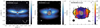 |
Fig. 1 High-resolution observations of PDS 453. The size of the corresponding PSF is shown in the bottom left corner of each panel, and the gray circles represent the size of coronagraphic masks. The red star corresponds to the position of the bright central point source. Left panel: VLT/SPHERE 1.6 µm polarized intensity image shown with a logarithmic stretch. Middle panel: HST/NICMOS scattered-light F110W total intensity image shown using a logarithmic stretch. Right panel: HST/NICMOS scattered-light 2 µm polarization fraction map along with polarization vectors. The polarization fraction is only computed in the area in which the total intensity is detected at the 1 σ level. All images have the same scale, 3 × 3 arcsec. |
2.2 Observational results
The SPHERE and NICMOS images presented here confirm that the disk around PDS 453 is highly inclined, as identified by Perrin et al. (2010). The outer radius of the disk is ≈1″.2, and a well-resolved dark lane bisects the two disk surfaces. The curved ring-like nature of the upper surface indicates that the disk is inclined at ~80°. Furthermore, this suggests a sharp transition in the disk density profile at a radius of ≈0″.5 (~70 au) from the star, similar to 2MASS J16083070-382826 (Villenave et al. 2019).
A bright central point source is observed along the top surface. This is a rare configuration among such highly inclined disks. This bright central point source is not visible in our observations because it was blocked by the coronagraph and subtracted as part of the data reduction process. To determine the nature of this component, we compiled the spectral energy distribution (SED) of the system. To this end, we complement existing optical through mid-infrared photometry from all-sky surveys available in VizieR2 with new far-infrared Herschel photometry. PDS 453 is included in one of the wide-field Spectral and Photometric Imaging Receiver (SPIRE) maps taken as part of the Herschel Gould Belt Survey Guaranteed Time Key Program (André et al. 2010). We retrieved the level 2.5 SPIRE (250, 350, and 500 µm) data products from the Herschel archive. PDS 453 is clearly detected in all three filters. Following the SPIRE handbook, we estimated the photometry for the system using Gaussian fitting and applying band-appropriate aperture corrections. This yielded flux densities of 1.30±0.06, 0.77±0.08, and 0.40±0.06Jy at 250, 350, and 500 µm, respectively. The resulting SED is shown in Figure 2. The optical photometry shows that the system is underluminous in the visible and nearinfrared compared to other F-type stars in Sco-Cen (Pecaut et al. 2012). This indicates that the central point source is a forwardscattering glint through the upper layer of the disk rather than a direct view of the star.
Moreover, the SED of the system is typical of so-called flat-spectrum sources (Greene et al. 1994). While these objects are generally understood as an intermediate evolutionary stage between embedded and revealed young stellar objects, edge- on disks around T Tauri stars can yield similarly shaped SEDs depending on their exact orientation, (e.g., Glauser et al. 2008). The images of PDS 453 do not indicate the presence of a remnant envelope, and we thus interpret it as a similar object. In other words, the system is viewed at a peculiar angle, at a grazing incidence through the upper layers of the disk. This enables us to directly trace its surface.
The 2 µm polarization fraction measured with NICMOS increases monotonously from ~20% at the edge of the coronagraphic mask to ~50% near the edge of the disk. We estimated these fractions by averaging the total and polarized intensity signals between two horizontal lines that bracket the spine of the top nebula. The orientation of the polarization vectors is orthoradial in all regions, consistent with scattering of stellar photons off dust grains (see the right panel of Fig. 1).
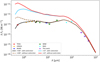 |
Fig. 2 Spectral energy distributions of the best model of PDS 453 with and without foreground extinction (solid black line with AV = 1.9 mag and dashed brown line, respectively). The SEDs of the same model viewed pole-on are shown with and without the same visual extinction (solid blue line and dashed red line, respectively). The upper limits are indicated with downward-pointing arrows (see Sect. 4 for a description of the models). |
3 Modeling setup
In this section, we describe a model that reproduces the various observational elements established in the previous section, namely the system SED, the 1.6 µm polarized intensity image, and the 2 µm polarization fraction map. While the model was not optimized for the 1.1 µm NICMOS total intensity image, it provides an additional constraint on the dust properties and is included for discussion.
We used the MCFOST radiative transfer code (Pinte et al. 2006), which produces synthetic SEDs, scattered-light images, and polarization maps, and we assumed that the disk is axisymmetric. The model exploration started from a setup designed by Perrin et al. (2010), which we modified to improve the global adjustment, in particular, to match the higher resolution of the SPHERE image. We caution that we did not attempt to obtain the best quantitative match to the data. We leave a detailed model fit to a future study. Nonetheless, as shown below, we achieved a satisfactory match to all key aspects of the selected observations.
We fixed the disk inclination to 80° based on the morphology of the SPHERE image. We used a photospheric spectrum to represent the star (Baraffe et al. 1998) and set the effective temperature of the star to 6810 K, which is appropriate for an F2- type star (Pecaut & Mamajek 2013), and the stellar luminosity to 8.69 L⊙, typical of early-F stars in the nearby Upper Centaurus Lupus star-forming region (Pecaut et al. 2012).
We initially considered a simple model, with a single surface density profile extending smoothly to the outer disk radius. However, this model produced a smooth image without the sharp ring seen in the SPHERE observation (see Fig. B.1). We therefore designed a model with two partially overlapping regions, and the outer region was characterized by a higher scale height and a higher degree of flaring. This combination was necessary to reproduce the scattered-light polarized intensity distribution. We note that two distinct regions are often necessary to reproduce observations of protoplanetary disks (e.g., Woitke et al. 2019; Kaeufer et al. 2023). Fig. 3 presents a sketch of the geometry we adopted for the PDS 453 disk.
We adopted a power-law distribution, Σ(R) ∝ Rp, with sharp edges for the surface density profile in the inner region. Conversely, we needed to use a tapered-edge profile,  , where Rc is a so-called critical radius, in the outer region. We assumed a Gaussian vertical density profile, which is appropriate for a vertically isothermal disk in hydrostatic equilibrium. The disk scale height is parametrized as
  , where β is the flaring index and R0 is an arbitrary reference radius that we set to 135 au. Each region has its inner and outer radius, Rin and Rout, and dust mass, Md.
We assumed that all grains are spherical and homogeneous. This allowed us to use the Mie theory. While it is numerically convenient, the Mie theory is known to reproduce scattered-light images only imperfectly (e.g., Min et al. 2012), as grains likely have more complex structures (Pinte et al. 2008; Tazaki et al. 2023). It is nonetheless widely used in the field (e.g., Birnstiel et al. 2018), and we adopted it because it does not alter our conclusions qualitatively. The grains are composed of a mixture of two solid species: dirty water ice that is mostly crystalline, as described in Li & Greenberg (1998), and a mixture of graphite, silicate, and amorphous carbon developed by Mathis & Whiffen (1989) to match the interstellar dust properties. We applied the Bruggeman rule effective medium theory (EMT) to compute the effective refractive index, including an additional level of porosity. We explored different proportions for the two species, with an ice volume fraction ranging from 5 to 50% in the outer disk region. In the inner region, we consistently assumed a lower ice proportion (by 10% in an absolute sense, or by half, whichever was smaller) than in the outer region. Finally, close to the star, the disk is warm enough to sublimate water ice. In a preliminary model, we found that the midplane temperature is higher than 90 K inside of 3.7 au, and we therefore removed all water ice inside of this radius for all models. To determine the depth of the water-ice band, we normalized the spectrum by a second- or third-order polynomial fit to the 1.65–2.3 µm and 4.0–4.6 µm continuum regions and obtained the relative depth of the band from its minimum.
We assumed a power-law grain size distribution n(a)da ∝a–qda, with q = 3.5 extending from amin = 0.03 µm to amax = 3000 µm, where the maximum grain size was set to match the long-wavelength end of the SED. The dust grains were assumed to be in radiative equilibrium and local thermodynamic equilibrium (LTE), as appropriate for an optically thick disk.
As we compared the resulting model images and SED to the observed images, we varied the mass, scale height, flaring index, surface density index, and radial extent of both regions, as well as the water-ice fraction through a manual exploration. All the model parameters (fixed and varied) are summarized in Table 2.
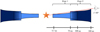 |
Fig. 3 Sketch of the PDS 453 model viewed at 80°. |
Parameters of the PDS 453 model.
4 Results
4.1 Disk morphology
The synthetic images and polarization map of our final model are presented in Fig. 4. The model satisfyingly matches all observations in terms of morphology (radius, aspect ratio, and presence of a bright ring), width of the dark lane, brightness ratio of the two nebulae, size, and maximum polarization. The outer disk radius is 160 au, as indicated by the extent of the SPHERE scattered-light image. The curved upper surface (above the dark lane in Fig. 1) and the flatter nature of the lower surface (below the dark lane) are well reproduced. As discussed in Sect. 2, the turnaround points toward the far side on the top surface suggest a ring-like structure, similar to a transition disk. However, the SED of the system shows infrared excess extending from 2 µm to the submillimeter regime, so that a fully cleared inner disk is ruled out. We note that the temperature of water-ice sublimation is reached at ~60 au at the surface of the disk in our model, suggesting that this transition could be due to the location of the snow line in the system. The lack of polarized intensity on the far side of the ring is well matched when porosity is included in our model.
The main shortcomings of our model are related to the lower nebula. In the SPHERE observation, the polarized intensity is fainter in the center than at the edges of the disk, whereas in the NICMOS 1.1 µm image, its radial extent is shorter than the upper nebula. Neither feature is well reproduced (see Fig. 4), suggesting that the scattering phase function and/or polarizability curves of the dust model we adopted are imperfect, possibly because we chose to use the Mie theory. Moreover, because the HST and SPHERE observations are separated by 10 years, another possible explanation is the change in illumination, for instance, as the result of a misaligned inner disk (e.g., Benisty et al. 2022).
Because of our grazing-angle perspective of the system, the disk surface is traced primarily by single-scattered photons. Still, the disk blocks our direct view of the star, such that the bright central point source we see is substantially fainter than the star itself. In our model, the central point source when the system is observed at an inclination of 80° has ~3% of the brightness of the star at 1.1 µm (as measured in a pole-on view of the same model).
Very few protoplanetary disks match this peculiar geometry. Most prominently, MY Lup, with an inclination of i = 73°, also presents a bright inner ring feature, a dark lane, and a bright central point source (Avenhaus et al. 2018). In this system, Jennings et al. (2022) demonstrated that the ring feature coincides with a trough in the submillimeter continuum emission. Unfortunately, no resolved submillimeter observations of PDS 453 exist to date. A few additional systems in other star-forming regions present similar morphologies: DoAr 25, V1012 Ori, PDS 111, V409 Tau, and RY Tau (Garufi et al. 2020; Valegård et al. 2024; Derkink et al. 2024; Garufi et al. 2024). They might represent a valuable coherent sample for future systematic studies.
4.2 Spectral energy distribution
The SED of the model (Fig. 2) matches the observed SED well when we include a foreground extinction of AV = 1.9 mag (assuming an extinction law characterized by Rv = 3.1). The extinction estimate we obtained is consistent with the low Galactic latitude of PDS 453. Esplin & Luhman (2020) estimated an extinction of AV = 2–3 mag for the stellar population of the nearby Upper Scorpius star-forming region. This is significantly higher than the extinction of Av = 0.1 mag estimated by Sartori et al. (2010). This difference arises because scattering off the circumstellar medium does not preserve the colors of the central source and therefore biases the extinction estimates.
The spectral index between 350 and 1000 µm of the model was estimated to be α = –2.1 using Fν ∝ να. This suggests that the disk is optically thick in this regime. Longer-wavelength observations in the millimeter regime are required to estimate this index empirically and confirm this conclusion.
The model presented here produces a relatively shallow water-ice absorption band around 3.1 µm. This qualitatively agrees with the observations of Terada & Tokunaga (2017). We note that the foreground extinction is too low to be expected to produce water-ice absorption, for which AV must be ≳3 mag according to Boogert et al. (2015), and that there is no evidence that a remnant envelope is associated with the system. We conclude that the water-ice band originates from the disk itself.
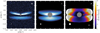 |
Fig. 4 Synthetic observations of our best PDS 453 model with two zones, with similar scales and stretches as in Fig. 1. All images have been convolved by the appropriate PSF after we subtracted the central point source to mimic the effect of the coronagraph. Left panel: scattered-light 1.6 µm polarized intensity image shown at the SPHERE resolution. Middle panel: scattered-light F110W total intensity image at the NICMOS resolution. Right panel: scattered-light 2 µm polarized fraction map. The polarization vectors are superimposed. The solid red line approximates the location of the spine of the top nebula. The two gray lines represent the vertical range over which the total and polarized intensities are measured to compute the polarized fraction shown in Fig. 9. |
4.3 Water-ice absorption band
Regardless of whether absorption or scattering dominates, the peculiar geometry of PDS 453 is such that we can conclude that water ice is present in disk layers that are located much above the midplane. This is despite the fact that in this layer, water ice could easily sublimate over a large fraction of the radial disk extent. Water-ice absorption is usually attributed to an effect of transmission of starlight through foreground material. However, in the case of highly inclined disks, where scattering dominates, the dust albedo spectrum becomes relevant and can also contribute significantly to the 3 µm water-ice band.
Our model produces a clear water-ice band (Fig. 2), although it does not perfectly match the observed band. Discrepancies in the detailed shape and central wavelength of the profile might arise from the assumed type of water ice. We considered amorphous ice, while Terada & Tokunaga (2017) used highly crystalline ice. As shown in Fig. 14 of Tazaki et al. (2021), there are significant differences in the refractive indices of these two types of ices. Moreover, Terada & Tokunaga (2017) measured a relative depth of the minimum of the water band of ~24%, taking into account the bias introduced by the limited wavelength range from their continuum estimate. In our model, the water-ice band is deeper, with a depth of ~33% relative to the continuum. A slightly lower inclination or ice content might improve this aspect (see Sect. 5.1), but it would come at the cost of poorer matches to the other observable quantities.
Finally, we note that the ice volume fraction used in our PDS 453 model 10–20% is similar to what is typically suggested from water-ice observations for disks in a wide range of inclinations (Pontoppidan et al. 2005; Tazaki et al. 2021; Sturm et al. 2023b, 2024). This value is significantly lower than the value that is often used to model the dust opacity in protoplanetary disks (Pollack et al. 1994; D’Alessio et al. 2001; Birnstiel et al. 2018), where a water-ice volume fraction of about 36–60% is assumed based on the solar abundances or cometary observations. The relatively low ice abundances in the disk surface might point to a disruption of water ice via nonthermal processes (Hollenbach et al. 2009; Oka et al. 2011), although a detail physical-chemical modeling (e.g., Ballering et al. 2021) is needed to clarify the origin.
4.4 Polarization fraction
The 2 µm polarization fraction increases with distance from the star in the model (Fig. 4, right panel), in agreement with the measured polarization fraction from the NICMOS data (Fig. 1, right panel). This effect is due to a scattering-angle effect: close to the star, the light is perceived as forward-scattering, while near the outer edge of the disk, the light is scattered at a 90° scattering angle. The latter generally produces higher polarization fractions. The pattern of polarization vectors in the model is centro-symmetric, consistent with the observations and with previous studies of nearly edge-on young stellar objects (Murakawa 2010).
The general behavior is satisfactorily reproduced by our model, with a continuous rise from the inside to the outside of the disk as well as the correct maximum polarization at the edge of the disk ≈40%. However, the model underpredicts the polarization fraction at small projected separations (see Sect. 5.1.2). Close to the star, this difference may be caused by imperfectly subtracted starlight leakage at the edge of the coronagraph and/or by the intrinsically biased nature of the polarization fraction. The difference could arise from a density profile with too sharp an edge compared to observations. Moreover, no noise was added in the HST image model. The difference in radius between the observations and our model arises from the fact that Rout of the model is based on the dimension of the disk as seen in the SPHERE image. However, in the polarization map based on the 2 µm NICMOS image, we defined the limited radius of the observations based on the detection limit of the 2 µm total intensity scattered-light image presented in Fig. A.1.
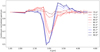 |
Fig. 5 Continuum-normalized synthetic model spectra centered around the water-ice band as a function of inclination. We only present every other inclination for clarity. The spectrum at 80° represents our best model of PDS 453. |
5 Discussion
The model we constructed reproduces the observations of PDS 453 despite small shortcomings and unsolved degeneracies inherent to such an exercise. In the absence of higher-resolution observations, in particular, with ALMA (a good tracer of the total mass of millimeter dust), we consider it premature to try and refine the model to fit the data with more accuracy. Nonetheless, we consider that the two-zone nature of our model, as well as the presence of water ice in the upper disk layers that absorbs and/or scatters light from the central star, are directly established from observations. Beyond the properties of this disk, we took advantage of our model to explore how the water-ice band and the polarization fraction are dependent on physical parameters in general, such as viewing angle, disk vertical structure, and dust properties.
5.1 Water-ice absorption band
5.1.1 Sensitivity to inclination
We explored the influence of the system inclination on the depth and spectral shape of the water-ice band. To this end, we started from our best PDS 453 model including star and disk and computed the emergent spectrum in the range 1.6–4.6 µm while varying the inclination from 75 to 90°, where i = 80° corresponds to the PDS 453 geometry (see Fig. 5). For i < 75°, the stellar photosphere of the central star is directly visible and no water-ice band is detected. Above this limit, in addition to an increase in the depth of the water-ice band, the spectral profile of the band varies with inclination. The minimum of the band shifts from ~3.1 µm ~to 2.9 µm as the inclination increases. Furthermore, the water-ice band is asymmetrical, with a wider wing that switches from the blue to the red side of band. The water-ice band is almost symmetrical at ~82°. Finally, there is a small bump over the continuum that also switches from the blue to the red side as the inclination increases.
The refractive index of water ice provides an explanation for this behavior with inclination. Fig. 6 shows the refractive index and opacity of water ice. Broadly speaking, the real and imaginary parts are linked to scattering and absorption, respectively. At intermediate inclinations (78-82°), where the optical depth through the disk is not negligible but moderate, absorption dominates scattering, and we essentially find a transmittance spectrum. Based on the absorption opacity curve, the waterice band is centered at ≳3.0 µm, as observed in our model. At even higher inclinations, the optical depth becomes so high that no photons are directly transmitted to the observer. The spectrum is then dominated by scattering. Since the minimum albedo occurs at ≈2.9 µm, this explains the shift to shorter wavelengths in our model. This behavior agrees with Boogert et al. (2015), who showed that detection of the water-ice band at 2.9 µm is indicative of scattering. In the case of PDS 453, the waterice band is located around 3.1 µm (Terada & Tokunaga 2017), which is therefore primarily linked to the absorption by water ice. This agrees with the assumption that the line of sight to the photosphere is at a grazing incidence on the disk surface, that is, at a moderate optical depth of 3.1 µm.
The asymmetry in the water-ice band wings may be explained in a similar manner. The blue wing at low inclinations is influenced by the wavelength dependence of the optical constants of the materials (McClure et al. 2023), whereas the asymmetry of the red wing is due to a strong scattering effect by large grains (Leger et al. 1983; Boogert et al. 2015). The fact that large grains produce this effect means that a distortion in ice bands may be an indicator of grain growth, with sizes well above the those in the ISM (Dartois et al. 2024).
5.1.2 Sensitivity to the water-ice abundance
The amount of ice also affects the depth of the water ice band. We varied the amount of water ice in the model and show the results in Fig. 7. Except for the water-ice proportion in both regions, all other model parameters remain unchanged. The water-ice band is detectable with the lowest volume fraction of ice we considered (2.5 and 5% in the inner and outer regions, respectively). In contrast to the variation in inclination, the wavelength of the water-ice band minimum does not depend on the ice content and remains at ≈3.0µm. The wings of the waterice band are symmetrical for low ice abundances and become asymmetrical with a more pronounced blue wing for higher ice abundances.
5.1.3 Implication for the interpretation of the depth of the water-ice band
Fig. 8 summarizes our findings about the dependence of the water-ice band on inclination and ice fraction. For our best PDS 453 model, the depth of the water-ice band rises sharply between 76 and 80° as the column density increases, but it reaches a nearly flat plateau at i ≳ 81° (edge-on disks). In other words, the water-ic e band reaches saturation beyond a critical inclination, where it becomes impossible to quantify the amount of water ice. This phenomenon was reported in models by Pontoppidan et al. (2005) and Sturm et al. (2023b), as well as in observations of the edge-on disk surrounding the L1527 protostar (Aikawa et al. 2012). While the critical inclination is dependent on the disk properties (mass, scale height, flaring, etc.), this saturation effect will be relevant in the interpretation of upcoming JWST observations of highly inclined disks. Moreover, the depth of the water-ice band evolves rapidly in the range of inclinations between ~79° and 81°, which means that a unique solution for the model is hard to obtain. In addition, while the spectrum we used only covers the water-ice band at 3.1 µm, other ice species can be detected in edge-on disks that also show asymmetric water-ice bands (e.g., Aikawa et al. 2012). For instance, CO2 presents two absorption ice bands at 4.27 and 15 µm, while CO features an ice band at 4.67 µm. We defer the modeling CO and CO2 ices in preparation of future PDS 453 observations to a subsequent paper.
This water-ice band saturation phenomenon is also observed as a function of the ice quantity (Fig. 8). In our best model for PDS 453, saturation occurs when the water-ice volume fraction reaches ∼40%. Sturm et al. (2023a) also found that the H2O, CO, and possibly CO2 ice bands are saturated in the HH 48 NE edge-on disk.
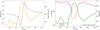 |
Fig. 6 Properties of water ice. Left panel: refractive indices of water ice from Li & Greenberg (1998). The real part is displayed on a linear scale, and the imaginary part is shown on a logarithmic scale. Right panel: opacities on a logarithmic scale, and albedo of water ice on a linear scale. |
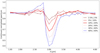 |
Fig. 7 Continuum-normalized synthetic model spectra centered around the water-ice band as a function of the volume fraction of ice in the disk. The spectrum with 10:20% of water-ice represents our best model of PDS 453. |
5.2 Dust properties
In addition to the water-ice band, the polarization map across the disk provides information on the dust properties. Our best model broadly reproduces the trend of the increasing polarization fraction as a function of projected distance from the star as well as the maximum polarization fraction of ∼40% (Fig. 9). In an attempt to alter the polarization fraction profile, we computed another model in which the maximum grain size was set to 50 µm instead of 3mm. Since our model assumed fully mixed dust, a reduced maximum grain size represents a simplified approach to incorporating dust settling, as the millimeter grains are known to be concentrated in a thin midplane where they cannot scatter starlight (Villenave et al. 2020). The resulting polarization fraction throughout the disk is slightly lower than what is observed, but the shape of the curve is unchanged. It is likely necessary to further reduce amax to obtain a better match. However, in fully mixed models, the long-wavelength end of the SED requires the presence of millimeter grains, and the models are much poorer overall matches to the observed properties of PDS 453. Models with settling would likely help us to solve this conundrum, but they are beyond the scope of this work.
Tazaki et al. (2019) suggested that a high polarization fraction of 65–75% indicates highly porous dust aggregates that consist of small monomer grains, whereas a lower polarization fraction of about 30% corresponds to more compact grains. Porosity, which we set at 50% in our model, strongly affects the way in which light is scattered off grains, in particular, it reduces back-scattering. In addition, the degree of polarization can also be affected by the composition and the monomer radius within the aggregates (Tazaki & Dominik 2022).
In addition to porosity, the shape of the grains also affects the polarization fraction. We adopted spherically homogeneous grains (Mie theory) for simplicity in this study. However, while little is known about the structure of dust particles in protoplan- etary disks, studies of Solar System particles clearly indicate that their aggregate nature is complex (Brownlee 1985; Bentley et al. 2016; Mannel et al. 2016). Tazaki et al. (2023) have studied the disk around IM Lup and demonstrated that these particles with a complex morphology, with a fractal dimension of ~1.5 and a characteristic radius greater than 2 µm, are necessary to reproduce observations. Considering particles like this in the case of PDS 453 may also help us to improve the match to observations.
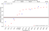 |
Fig. 8 Variations in the relative depth of the water-ice band as a function of the system inclination and the ice quantity. All model parameters remain unchanged, except for the inclination for the red dots and ice quantities for the blue dots. The horizontal dashed red line indicates the measured band depth (Terada & Tokunaga 2017). |
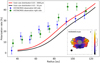 |
Fig. 9 Observed (data points) and model (curves) polarization fraction measured along the top disk surface from the edge of the coronagraphic mask to the outer edge of the disk. The red and black model curves only differ by the maximum grain size, with amax = 3000 and 50 µm, respectively. The inset presents the same image as in Fig. 4, and the solid blue and green lines correspond to the radius along which the polarization rate is measured. The limits between the average pixel values are represented by the two dashed gray lines. |
6 Conclusions
We have presented new high-resolution near-infrared polarized intensity, total intensity, and linear polarization fraction images of the PDS 453 protoplanetary disk. We developed a radiative transfer model that adequately reproduced the geometry and size of the disk in the SPHERE image, the behavior of the polarization map from the NICMOS observation, and the system SED and depth of the 3.1 µm water-ice band. Our main conclusions are listed below.
The surface density profile of PDS 453 extends from near the stellar surface to 160 au, with a sharp transition at 70 au that produces a clear ring-like feature in the SPHERE image. Our model incorporates this as two distinct regions. The location of this transition roughly matches that of the water snow line in the upper disk surface.
The PDS 453 disk is inclined at 80° which results in combination with the disk scale height in a rare configuration in which our line of sight to the star grazes the disk upper surface. The bright central point source that is observed in the system, which is much fainter than the star itself, is best interpreted as a forward-scattering glint. This particular viewing geometry, in combination with a modest amount of foreground extinction, also accounts for the flat SED of the system from the optical to 100 µm.
The disk of PDS 453 is composed of a mixture of dust and water ice. This accounts for the observed absorption band at 3.1 µm. In our model, the inner and outer disk contain 10 and 20% by volume of water ice assuming Mie theory. Our dust mixture also reproduces the fact that we partially detect the far side of the 70 au ring in polarized intensity, as well as the observed near-infrared polarization fraction.
Exploring variations in inclination and water-ice content from the best model for the PDS 453, we found that the central wavelength, spectral shape, and depth of the 3.1 µm water-ice band result from a balance between absorption and scattering. In particular, for disks seen at a grazing angle (like PDS 453) or higher inclinations, we found that the depth of the water-ice band easily saturates when the column density through the line of sight becomes too high. This effect constitutes a barrier to the quantification of the water ice within highly inclined disks and will affect forthcoming edge-on disk observations by JWST. In general, it will only be possible to place a lower limit on the water-ice content of these disks.
Observations from JWST and ALMA are expected to provide new images to constrain more parameters and thus to improve the PDS 453 model presented here. From a JWST spectrum, it will be possible to obtain ice profiles, notably CO and CO2, which are currently unknown for this source. ALMA will notably help us to constrain the mass and inclination of the disk, which are two crucial parameters for building more accurate models.
Understanding the vertical structure through the study of edge-on disks and how grains grow is crucial to our understanding of planetary formation mechanisms.
Acknowledgements
This project has received funding from the European Research Council (ERC) under the European Union’s Horizon Europe research and innovation program (grant agreement No. 101053020, project Dust2Planets, PI: F. Ménard and grant agreement No. 101002188, project PROTOPLANETS, PI: M. Benisty). K.R.S., G.D., and S.G.W. acknowledge funding support from JWST GO program #2562 provided by NASA through a grant from the Space Telescope Science Institute, which is operated by the Association of Universities for Research in Astronomy, Incorporated, under NASA contract NAS5-26555. We are thankful to John P. Wisniewski for his help with the NICMOS data and discussion about the paper. We are thankful to Gaël Chauvin for the overall management of the SPHERE GTO survey. SPHERE was designed and built by a consortium made of IPAG (Grenoble, France), MPIA (Heidelberg, Germany), LAM (Marseille, France), LESIA (Paris, France), Laboratoire Lagrange (Nice, France), INAF–Osservatorio di Padova (Italy), Observatoire de Genève (Switzerland), ETH Zurich (Switzerland), NOVA (Netherlands), ONERA (France) and ASTRON (Netherlands) in collaboration with ESO. SPHERE was funded by ESO, with additional contributions from CNRS (France), MPIA (Germany), INAF (Italy), FINES (Switzerland) and NOVA (Netherlands).
Appendix A HST/NICMOS total intensity and polarization intensity image at 2 µm
Figure A.1 presents the 2 µm HST/NICMOS scattered-light total intensity and polarized intensity images.
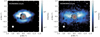 |
Fig. A.1 Observations of PDS 453. The size of the corresponding PSF is shown in the bottom left corner of each panel, and the gray circles represent the size of coronagraphic masks. The red star corresponds to the position of the bright central point source. Left panel: HST/NICMOS scattered-light total intensity image at 2 µm shown using a logarithmic stretch. Right panel: HST/NICMOS scattered-light polarized intensity image 2 µm shown using a logarithmic stretch. |
Appendix B Single-zone model
In Figure B.1, we present the same model as PDS 453 but with only one zone defined between Rin = 0.2 au and Rout = 160 au. The dust mass is Md = 1.8 × 10⁻⁵ M⊙, the scale height is fixed at H0 = 8.5 au, the flaring index at β = 1.13 and the surface density at P = –1.
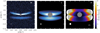 |
Fig. B.1 Synthetic observations of our PDS 453 model with a single zone, with similar scales and stretches as in Fig. 1 and Fig. 4. All images have been convolved by the appropriate PSF after subtracting the central point source to mimic the effect of the coronagraph. Left panel: Scattered-light 1.6 µm polarized intensity image shown a the SPHERE resolution. Middle panel: Scattered-light F110W total intensity image at the NICMOS resolution. Right panel: Scattered-light 2 µm polarized fraction map with polarization vectors superimposed. |
References
- Aikawa, Y., Kamuro, D., Sakon, I., et al. 2012, A&A, 538, A57 [NASA ADS] [CrossRef] [EDP Sciences] [Google Scholar]
- André, P., Men’shchikov, A., Bontemps, S., et al. 2010, A&A, 518, L102 [NASA ADS] [CrossRef] [EDP Sciences] [Google Scholar]
- Andrews, S. M., Huang, J., Pérez, L. M., et al. 2018, ApJ, 869, L41 [NASA ADS] [CrossRef] [Google Scholar]
- Avenhaus, H., Quanz, S. P., Garufi, A., et al. 2018, ApJ, 863, 44 [NASA ADS] [CrossRef] [Google Scholar]
- Ballering, N. P., Cleeves, L. I., & Anderson, D. E. 2021, ApJ, 920, 115 [NASA ADS] [CrossRef] [Google Scholar]
- Baraffe, I., Chabrier, G., Allard, F., & Hauschildt, P. H. 1998, A&A, 337, 403 [Google Scholar]
- Bentley, M. S., Schmied, R., Mannel, T., et al. 2016, Nature, 537, 73 [Google Scholar]
- Benisty, M., Dominik, C., Follette, K., et al. 2022, Protostars and Planets VII, Optical and Near-infrared View of Planet-forming Disks and Protoplanets (Tucson: University of Arizona Press) [Google Scholar]
- Benisty, M., Dominik, C., Follette, K., et al. 2023, ASP Conf. Ser., 534, 605 [NASA ADS] [Google Scholar]
- Beuzit, J. L., Vigan, A., Mouillet, D., et al. 2019, A&A, 631, A155 [NASA ADS] [CrossRef] [EDP Sciences] [Google Scholar]
- Birnstiel, T., Dullemond, C. P., Zhu, Z., et al. 2018, ApJ, 869, L45 [CrossRef] [Google Scholar]
- Boogert, A. C. A., Gerakines, P. A., & Whittet, D. C. B. 2015, ARA&A, 53, 541 [Google Scholar]
- Brownlee, D. E. 1985, Ann. Rev. Earth Planet. Sci., 13, 147 [Google Scholar]
- Burrows, C. J., Stapelfeldt, K. R., Watson, A. M., et al. 1996, ApJ, 473, 437 [Google Scholar]
- D’Alessio, P., Calvet, N., & Hartmann, L. 2001, ApJ, 553, 321 [Google Scholar]
- Dartois, E., Noble, J. A., Caselli, P., et al. 2024, Nature Astronomy, 8, 359 [NASA ADS] [CrossRef] [Google Scholar]
- de Boer, J., Langlois, M., van Holstein, R. G., et al. 2020, A&A, 633, A63 [NASA ADS] [CrossRef] [EDP Sciences] [Google Scholar]
- Derkink, A., Ginski, C., Pinilla, P., et al. 2024, A&A, 688, A149 [NASA ADS] [CrossRef] [EDP Sciences] [Google Scholar]
- Dohlen, K., Langlois, M., Saisse, M., et al. 2008, SPIE Conf. Ser., 7014, 70143L [Google Scholar]
- Duchêne, G., Ménard, F., Stapelfeldt, K. R., et al. 2024, AJ, 167, 77 [CrossRef] [Google Scholar]
- Esplin, T. L., & Luhman, K. L. 2020, AJ, 159, 282 [Google Scholar]
- Garufi, A., Avenhaus, H., Pérez, S., et al. 2020, A&A, 633, A82 [NASA ADS] [CrossRef] [EDP Sciences] [Google Scholar]
- Garufi, A., Ginski, C., van Holstein, R. G., et al. 2024, A&A, 685, A53 [NASA ADS] [CrossRef] [EDP Sciences] [Google Scholar]
- Glauser, A. M., Ménard, F., Pinte, C., et al. 2008, A&A, 485, 531 [NASA ADS] [CrossRef] [EDP Sciences] [Google Scholar]
- Greene, T. P., Wilking, B. A., Andre, P., Young, E. T., & Lada, C. J. 1994, ApJ, 434, 614 [NASA ADS] [CrossRef] [Google Scholar]
- Hines, D. C., Schmidt, G. D., & Schneider, G. 2000, AAS Meeting Abstracts, 197, 12.10 [NASA ADS] [Google Scholar]
- Hollenbach, D., Kaufman, M. J., Bergin, E. A., & Melnick, G. J. 2009, ApJ, 690, 1497 [NASA ADS] [CrossRef] [Google Scholar]
- Jennings, J., Tazzari, M., Clarke, C. J., Booth, R. A., & Rosotti, G. P. 2022, MNRAS, 514, 6053 [NASA ADS] [CrossRef] [Google Scholar]
- Johansen, A., Blum, J., Tanaka, H., et al. 2014, in Protostars and Planets VI, eds. H. Beuther, R. S. Klessen, C. P. Dullemond, & T. Henning (Tucson: University of Arizona Press), 547 [Google Scholar]
- Kaeufer, T., Woitke, P., Min, M., Kamp, I., & Pinte, C. 2023, A&A, 672, A30 [NASA ADS] [CrossRef] [EDP Sciences] [Google Scholar]
- Keppler, M., Benisty, M., Müller, A., et al. 2018, A&A, 617, A44 [NASA ADS] [CrossRef] [EDP Sciences] [Google Scholar]
- Leger, A., Gauthier, S., Defourneau, D., & Rouan, D. 1983, A&A, 117, 164 [NASA ADS] [Google Scholar]
- Li, A., & Greenberg, J. M. 1998, A&A, 331, 291 [NASA ADS] [Google Scholar]
- Long, F., Pinilla, P., Herczeg, G. J., et al. 2018, ApJ, 869, 17 [Google Scholar]
- Maire, A.-L., Langlois, M., Dohlen, K., et al. 2016, SPIE Conf. Ser., 9908, 990834 [Google Scholar]
- Mannel, T., Bentley, M. S., Schmied, R., et al. 2016, MNRAS, 462, S304 [NASA ADS] [CrossRef] [Google Scholar]
- Mathis, J. S., & Whiffen, G. 1989, ApJ, 341, 808 [Google Scholar]
- McClure, M. K., Rocha, W. R. M., Pontoppidan, K. M., et al. 2023, Nat. Astron., 7, 431 [NASA ADS] [CrossRef] [Google Scholar]
- Min, M., Canovas, H., Mulders, G. D., & Keller, C. U. 2012, A&A, 537, A75 [NASA ADS] [CrossRef] [EDP Sciences] [Google Scholar]
- Murakawa, K. 2010, A&A, 518, A63 [NASA ADS] [CrossRef] [EDP Sciences] [Google Scholar]
- Oka, A., Nakamoto, T., & Ida, S. 2011, ApJ, 738, 141 [Google Scholar]
- Pecaut, M. J., & Mamajek, E. E. 2013, ApJS, 208, 9 [Google Scholar]
- Pecaut, M. J., Mamajek, E. E., & Bubar, E. J. 2012, ApJ, 746, 154 [Google Scholar]
- Perrin, M. D. 2006, PhD thesis, University of California, Berkeley, USA [Google Scholar]
- Perrin, M. D., Schneider, G., Duchene, G., et al. 2009, ApJ, 707, L132 [Google Scholar]
- Perrin, M. D., Schnieder, G., Duchene, G., et al. 2010, AAS Meeting Abs., 215, 428.12 [Google Scholar]
- Pinte, C., Ménard, F., Duchêne, G., & Bastien, P. 2006, A&A, 459, 797 [NASA ADS] [CrossRef] [EDP Sciences] [Google Scholar]
- Pinte, C., Padgett, D. L., Ménard, F., et al. 2008, A&A, 489, 633 [NASA ADS] [CrossRef] [EDP Sciences] [Google Scholar]
- Pollack, J., Hollenbach, D., Beckwith, S., et al. 1994, ApJ, 421, 615 [NASA ADS] [CrossRef] [Google Scholar]
- Pontoppidan, K. M., Dullemond, C. P., van Dishoeck, E. F., et al. 2005, ApJ, 622, 463 [NASA ADS] [CrossRef] [Google Scholar]
- Preibisch, T., & Mamajek, E. 2008, Handbook of Star Forming Regions, The Nearest OB Association: Scorpius-Centaurus (Sco OB2) (USA: ASP Books) [Google Scholar]
- Ratzenböck, S., Großschedl, J. E., Alves, J., et al. 2023, A&A, 678, A71 [NASA ADS] [CrossRef] [EDP Sciences] [Google Scholar]
- Sartori, M. J., Gregorio-Hetem, J., Rodrigues, C. V., Hetem, A., & Batalha, C. 2010, AJ, 139, 27 [NASA ADS] [CrossRef] [Google Scholar]
- Schneider, G., Silverstone, M. D., & Hines, D. C. 2005, ApJ, 629, L117 [NASA ADS] [CrossRef] [Google Scholar]
- Sturm, J. A., McClure, M. K., Beck, T. L., et al. 2023a, A&A, 679, A138 [NASA ADS] [CrossRef] [EDP Sciences] [Google Scholar]
- Sturm, J. A., McClure, M. K., Bergner, J. B., et al. 2023b, A&A, 677, A18 [NASA ADS] [CrossRef] [EDP Sciences] [Google Scholar]
- Sturm, J. A., McClure, M. K., Law, C. J., et al. 2023c, A&A, 677, A17 [NASA ADS] [CrossRef] [EDP Sciences] [Google Scholar]
- Sturm, J. A., McClure, M. K., Harsono, D., et al. 2024, A&A, 689, A92 [NASA ADS] [CrossRef] [EDP Sciences] [Google Scholar]
- Tazaki, R., & Dominik, C. 2022, A&A, 663, A57 [NASA ADS] [CrossRef] [EDP Sciences] [Google Scholar]
- Tazaki, R., Tanaka, H., Kataoka, A., Okuzumi, S., & Muto, T. 2019, ApJ, 885, 52 [Google Scholar]
- Tazaki, R., Murakawa, K., Muto, T., Honda, M., & Inoue, A. K. 2021, ApJ, 921, 173 [NASA ADS] [CrossRef] [Google Scholar]
- Tazaki, R., Ginski, C., & Dominik, C. 2023, ApJ, 944, L43 [NASA ADS] [CrossRef] [Google Scholar]
- Terada, H., & Tokunaga, A. T. 2017, ApJ, 834, 115 [NASA ADS] [CrossRef] [Google Scholar]
- Valegård, P. G., Ginski, C., Derkink, A., et al. 2024, A&A, 685, A54 [NASA ADS] [CrossRef] [EDP Sciences] [Google Scholar]
- van Holstein, R. G., Girard, J. H., de Boer, J., et al. 2020, A&A, 633, A64 [NASA ADS] [CrossRef] [EDP Sciences] [Google Scholar]
- Villenave, M., Benisty, M., Dent, W. R. F., et al. 2019, A&A, 624, A7 [NASA ADS] [CrossRef] [EDP Sciences] [Google Scholar]
- Villenave, M., Ménard, F., Dent, W. R. F., et al. 2020, A&A, 642, A164 [EDP Sciences] [Google Scholar]
- Villenave, M., Stapelfeldt, K. R., Duchêne, G., et al. 2024, ApJ, 961, 95 [NASA ADS] [CrossRef] [Google Scholar]
- Vioque, M., Oudmaijer, R. D., Baines, D., Mendigutía, I., & Pérez-Martínez, R. 2018, A&A, 620, A128 [NASA ADS] [CrossRef] [EDP Sciences] [Google Scholar]
- Watson, A. M., & Stapelfeldt, K. R. 2007, AJ, 133, 845 [NASA ADS] [CrossRef] [Google Scholar]
- Woitke, P., Kamp, I., Antonellini, S., et al. 2019, PASP, 131, 064301 [NASA ADS] [CrossRef] [Google Scholar]
All Tables
All Figures
|
Fig. 1 High-resolution observations of PDS 453. The size of the corresponding PSF is shown in the bottom left corner of each panel, and the gray circles represent the size of coronagraphic masks. The red star corresponds to the position of the bright central point source. Left panel: VLT/SPHERE 1.6 µm polarized intensity image shown with a logarithmic stretch. Middle panel: HST/NICMOS scattered-light F110W total intensity image shown using a logarithmic stretch. Right panel: HST/NICMOS scattered-light 2 µm polarization fraction map along with polarization vectors. The polarization fraction is only computed in the area in which the total intensity is detected at the 1 σ level. All images have the same scale, 3 × 3 arcsec. |
| In the text | |
|
Fig. 2 Spectral energy distributions of the best model of PDS 453 with and without foreground extinction (solid black line with AV = 1.9 mag and dashed brown line, respectively). The SEDs of the same model viewed pole-on are shown with and without the same visual extinction (solid blue line and dashed red line, respectively). The upper limits are indicated with downward-pointing arrows (see Sect. 4 for a description of the models). |
| In the text | |
|
Fig. 3 Sketch of the PDS 453 model viewed at 80°. |
| In the text | |
|
Fig. 4 Synthetic observations of our best PDS 453 model with two zones, with similar scales and stretches as in Fig. 1. All images have been convolved by the appropriate PSF after we subtracted the central point source to mimic the effect of the coronagraph. Left panel: scattered-light 1.6 µm polarized intensity image shown at the SPHERE resolution. Middle panel: scattered-light F110W total intensity image at the NICMOS resolution. Right panel: scattered-light 2 µm polarized fraction map. The polarization vectors are superimposed. The solid red line approximates the location of the spine of the top nebula. The two gray lines represent the vertical range over which the total and polarized intensities are measured to compute the polarized fraction shown in Fig. 9. |
| In the text | |
|
Fig. 5 Continuum-normalized synthetic model spectra centered around the water-ice band as a function of inclination. We only present every other inclination for clarity. The spectrum at 80° represents our best model of PDS 453. |
| In the text | |
|
Fig. 6 Properties of water ice. Left panel: refractive indices of water ice from Li & Greenberg (1998). The real part is displayed on a linear scale, and the imaginary part is shown on a logarithmic scale. Right panel: opacities on a logarithmic scale, and albedo of water ice on a linear scale. |
| In the text | |
|
Fig. 7 Continuum-normalized synthetic model spectra centered around the water-ice band as a function of the volume fraction of ice in the disk. The spectrum with 10:20% of water-ice represents our best model of PDS 453. |
| In the text | |
|
Fig. 8 Variations in the relative depth of the water-ice band as a function of the system inclination and the ice quantity. All model parameters remain unchanged, except for the inclination for the red dots and ice quantities for the blue dots. The horizontal dashed red line indicates the measured band depth (Terada & Tokunaga 2017). |
| In the text | |
|
Fig. 9 Observed (data points) and model (curves) polarization fraction measured along the top disk surface from the edge of the coronagraphic mask to the outer edge of the disk. The red and black model curves only differ by the maximum grain size, with amax = 3000 and 50 µm, respectively. The inset presents the same image as in Fig. 4, and the solid blue and green lines correspond to the radius along which the polarization rate is measured. The limits between the average pixel values are represented by the two dashed gray lines. |
| In the text | |
|
Fig. A.1 Observations of PDS 453. The size of the corresponding PSF is shown in the bottom left corner of each panel, and the gray circles represent the size of coronagraphic masks. The red star corresponds to the position of the bright central point source. Left panel: HST/NICMOS scattered-light total intensity image at 2 µm shown using a logarithmic stretch. Right panel: HST/NICMOS scattered-light polarized intensity image 2 µm shown using a logarithmic stretch. |
| In the text | |
|
Fig. B.1 Synthetic observations of our PDS 453 model with a single zone, with similar scales and stretches as in Fig. 1 and Fig. 4. All images have been convolved by the appropriate PSF after subtracting the central point source to mimic the effect of the coronagraph. Left panel: Scattered-light 1.6 µm polarized intensity image shown a the SPHERE resolution. Middle panel: Scattered-light F110W total intensity image at the NICMOS resolution. Right panel: Scattered-light 2 µm polarized fraction map with polarization vectors superimposed. |
| In the text | |
Current usage metrics show cumulative count of Article Views (full-text article views including HTML views, PDF and ePub downloads, according to the available data) and Abstracts Views on Vision4Press platform.
Data correspond to usage on the plateform after 2015. The current usage metrics is available 48-96 hours after online publication and is updated daily on week days.
Initial download of the metrics may take a while.