| Issue |
A&A
Volume 676, August 2023
|
|
|---|---|---|
| Article Number | A33 | |
| Number of page(s) | 17 | |
| Section | Extragalactic astronomy | |
| DOI | https://doi.org/10.1051/0004-6361/202346441 | |
| Published online | 02 August 2023 | |
Radial velocities and stellar population properties of 56 MATLAS dwarf galaxies observed with MUSE
1
Institute of Physics, Laboratory of Astrophysics, École Polytechnique Fédérale de Lausanne (EPFL), 1290 Sauverny, Switzerland
e-mail: This email address is being protected from spambots. You need JavaScript enabled to view it.
2
Institut für Astro- und Teilchenphysik, Universität Innsbruck, Technikerstraße 25/8, Innsbruck 6020, Austria
3
Observatoire Astronomique de Strasbourg (ObAS), Université de Strasbourg – CNRS, UMR 7550 Strasbourg, France
4
UK Astronomy Technology Centre, Royal Observatory, Blackford Hill, Edinburgh EH9 3HJ, UK
5
Space Physics and Astronomy Research Unit, University of Oulu, PO Box 3000 90014 Oulu, Finland
6
Department of Astronomy and Center for Galaxy Evolution Research, Yonsei University, Seoul 03722, South Korea
7
Youngstown State University, One University Plaza, Youngstown, OH 44555, USA
Received:
17
March
2023
Accepted:
3
May
2023
Abstract
Dwarf galaxies have been extensively studied in the Local Group, in nearby groups, and selected clusters, giving us a robust picture of their global stellar and dynamical properties, such as their circular velocity, stellar mass, surface brightness, age, and metallicity in particular locations in the Universe. Intense study of these properties has revealed correlations between them, called the scaling relations, including the well-known universal stellar mass-metallicity relation. However, since dwarfs play a role in a vast range of different environments, much can be learned about galaxy formation and evolution through extending the study of these objects to various locations. We present MUSE spectroscopy of a sample of 56 dwarf galaxies as a follow-up to the MATLAS survey in low- to moderate-density environments beyond the Local Volume. The dwarfs have stellar masses in the range of M*/M⊙ = 106.1–109.4 and show a distance range of D = 14–148 Mpc, the majority of which (75%) are located in the range targeted by the MATLAS survey (10–45 Mpc). We thus report a 75% success rate for the semi-automatic identification of dwarf galaxies (79% for dwarf ellipticals) in the MATLAS survey on the subsample presented here. Using pPXF full spectrum fitting, we determine their line-of-sight velocity and can match the majority of them with their massive host galaxy. Due to the observational setup of the MATLAS survey, the dwarfs are located in the vicinity of massive galaxies. Therefore, we are able to confirm their association through recessional velocity measurements. Close inspection of their spectra reveals that ∼30% show clear emission lines, and thus star formation activity. We estimate their stellar population properties (age and metallicity) and compare our results with other works investigating Local Volume and cluster dwarf galaxies. We find that the dwarf galaxies presented in this work show a systematic offset from the universal stellar mass-metallicity relation toward lower metallicities at the same stellar mass. A similar deviation is present in other works in the stellar mass range probed in this work and might be attributed to the use of different methodologies for deriving the metallicity.
Key words: galaxies: dwarf / galaxies: stellar content / dark matter / cosmology: observations
© The Authors 2023
 Open Access article, published by EDP Sciences, under the terms of the Creative Commons Attribution License (https://creativecommons.org/licenses/by/4.0), which permits unrestricted use, distribution, and reproduction in any medium, provided the original work is properly cited.
This article is published in open access under the Subscribe to Open model. This email address is being protected from spambots. You need JavaScript enabled to view it. to support open access publication.
1. Introduction
Dwarf galaxies are regarded as the oldest and most numerous galaxy type in the Universe (Binggeli et al. 1990; Ferguson & Binggeli 1994), responsible for the formation of the more luminous and higher mass galaxies we see today (Frenk & White 2012). They are typically defined as galaxies with stellar masses ≤109 M⊙ (Bullock & Boylan-Kolchin 2017), small physical sizes, and magnitudes fainter than −17 mag in the V-band (Tammann 1994; Tolstoy et al. 2009).
Since most dwarf galaxies have low surface brightness they are elusive when compared to massive host galaxies. Thus, their study has been limited by instrumental constraints for a long time, leading to well-studied populations only in the Local Group (LG; e.g., Mateo 1998; Martin et al. 2006, 2016; Ibata et al. 2007, 2014; Koposov et al. 2008; Bell et al. 2011; McConnachie 2012; McConnachie et al. 2018, 2009; Simon 2019; Drlica-Wagner et al. 2020) and a few nearby groups in the Local Volume (LV; D ≲ 10 Mpc; e.g., Chiboucas et al. 2013; Danieli et al. 2017; Crnojević et al. 2019; Carlsten et al. 2019; Bennet et al. 2020; Müller et al. 2021b), and some galaxy clusters (e.g., Ferrarese et al. 2012; Eigenthaler et al. 2018; Venhola et al. 2019). In order to model and understand galaxy formation and evolution across cosmic time, it is essential to answer the question of whether the dwarfs studied in the Local Volume are representative of dwarfs in the nearby Universe at large.
Even though galaxy formation and evolution is thought to depend on a number of different factors and processes, galaxies show remarkably tight correlations between some of their basic stellar and dynamical properties (e.g., Binggeli & Jerjen 1997; Tassis et al. 2008). These scaling relations have been extensively studied for different galaxy types, in a range of environments, and in particular in light of a possible evolution with time (see, e.g., D’Onofrio et al. 2021, for a recent review). A few examples of well-established galaxy scaling relations are the velocity-luminosity or Tully-Fisher relation (Tully & Fisher 1977; Courteau et al. 2007), the Faber-Jackson relation (Faber & Jackson 1976), the Kormendy relation (Kormendy 1977), the fundamental plane of galaxies (e.g., Djorgovski & Davis 1987; Dressler et al. 1987; Cappellari et al. 2006; La Barbera et al. 2008), the bulge-to-black hole mass relation (Magorrian et al. 1998) and the mass-radius relation (Chiosi et al. 2020).
The mass-metallicity relation (MZR) is another long-known and well-studied scaling relation that exists for both gas and stellar metallicities (see, e.g., Maiolino & Mannucci 2019, for a recent review). Stellar spectroscopy and the analysis of color-magnitude diagrams first revealed this connection in nearby elliptical galaxies (McClure & van den Bergh 1968; Sandage 1972; Mould et al. 1983; Buonanno et al. 1985). An analysis of the Sloan Digital Sky Survey (SDSS) optical spectra has shown that this relation persists in galaxies with stellar masses in the range M*/M⊙ = 109–1012 for stellar and gas metallicities (Tremonti et al. 2004; Gallazzi et al. 2005, 2006; Lee et al. 2006; Panter et al. 2008; Mannucci et al. 2010; González Delgado et al. 2014). The study of this correlation was extended to dwarf galaxies in the LG, where Kirby et al. (2013) found that dwarf galaxies follow the same stellar MZR as more massive galaxies. This result was also found in semi-analytical galaxy formation and evolution models (SAMs) by several authors (e.g., Li et al. 2010; Font et al. 2011; Hou et al. 2014; Lu et al. 2014, 2017). Xia & Yu (2019a,b) demonstrate that the relation is universal in SAMs for different types of galaxies and over a large range of stellar (M*/M⊙ ∼ 103–1011) and dark matter halo masses (Mhalo/M⊙ ∼ 109–1015 h−1).
There are various mechanisms that potentially drive the MZR and have been discussed in the literature (see Maiolino & Mannucci 2019, and references therein). The most important ones are outflows due to stellar feedback (e.g., Garnett 2002; Brooks et al. 2007); downsizing (e.g., Cowie et al. 1996); low-mass galaxies being in an earlier evolutionary stage, and therefore showing larger gas fractions (e.g., Erb et al. 2006); a potentially mass-dependent initial mass function for higher mass galaxies (e.g., Köppen et al. 2007; Trager et al. 2000; Mollá et al. 2015; Vincenzo et al. 2016; Lian et al. 2018); and finally metal rich accreted gas from a previous burst of star formation in higher mass systems compared to lower mass ones (Brook et al. 2014; Ma et al. 2016).
In addition to the mass of a galaxy, its environment is one of the main independent factors when it comes to galaxy evolution, and as such has been studied extensively in the context of the MZR (Trager et al. 2000; Kuntschner et al. 2001; Thomas et al. 2005, 2010; Sheth et al. 2006; Sánchez-Blázquez et al. 2006; Pasquali et al. 2010; Zhang et al. 2018). It has been found that while the environment has a significant influence on the morphology, age, and star formation activity of a galaxy, its direct contribution to the shape of the MZR is small (Thomas et al. 2010; Mouhcine et al. 2011; Fitzpatrick & Graves 2015; Sybilska et al. 2017). Peng et al. (2015) and Trussler et al. (2020), however, find that dwarf satellite galaxies in high-density environments are more metal rich compared to dwarfs residing in lower density environments. This observation is attributed to the process of starvation (i.e., the lack of cold gas accretion in these high-density regions).
One caveat when calculating the MZR and comparing it with results from other works is the variety of methods that can be used to determine the metallicity (e.g., Kewley & Ellison 2008). Another important factor in the context of this work is that there have been few studies investigating the MZR in the dwarf galaxy mass regime (Lequeux et al. 1979; Lee et al. 2006; Vaduvescu et al. 2007; Zahid et al. 2012; Kirby et al. 2013; Andrews & Martini 2013), and these have mostly been limited to the LG. Therefore, increasing the sample size of dwarf galaxies in different environments will greatly benefit these discussions. In recent years there has been a great effort to advance our knowledge of dwarf galaxies beyond the boundaries of the LG (e.g., Irwin et al. 2009; Stierwalt et al. 2009; Kim et al. 2011; Chiboucas et al. 2013; Bennet et al. 2017; Danieli et al. 2017; Park et al. 2017; Cohen et al. 2018; Crnojević et al. 2019; Müller & Jerjen 2020; Davis et al. 2021; Drlica-Wagner et al. 2021; Müller et al. 2021b; Mutlu-Pakdil et al. 2022; Carlsten et al. 2022) and farther beyond the LV (e.g., Geha et al. 2017; Greco et al. 2018; Zaritsky et al. 2019; Habas et al. 2020; Su et al. 2021; Prole et al. 2021; Tanoglidis et al. 2021; Mao et al. 2021; La Marca et al. 2022). The MATLAS survey (Duc et al. 2015; Bílek et al. 2020), the basis for this study, is among the latter and delivers a large number (2210) of newly discovered dwarf galaxies beyond the LV. The vast majority of the dwarf galaxies identified in the MATLAS fields around ∼140 targeted early-type galaxies (ETGs), however, only have photometric data, and thus their distance, satellite nature, and environment is uncertain. In the case of the M101 group in the Local Volume, it has been shown that ∼80% of the candidates in a dwarf catalog have been contaminants (Bennet et al. 2017, 2019). However, due to a careful detection and selection procedure (see Habas et al. 2020), the degree of contamination in the MATLAS dwarf catalog is likely significantly lower. In order to advance our understanding of structure formation as a function of the environment, it is therefore of great importance to obtain distance or recessional velocity estimates for dwarf galaxies in order to confirm their dwarf and satellite nature.
In this study we aim to add information about line-of-sight velocities of dwarf galaxies identified in the MATLAS fields beyond the LV and to compare their extracted stellar population properties with results from other studies. This information contributes to the connection between host halo and number of subhalos (e.g., Kim et al. 2018; Nadler et al. 2019; Munshi et al. 2021), the morphology-density relation, the role the environment plays in the formation and evolution of dwarf galaxies (e.g., Ferguson et al. 1990; McConnachie 2012; Ferguson & Sandage 1989; Sawala et al. 2012; Steyrleithner et al. 2020); the discussion on phase-space correlations in dwarf satellites (e.g., Kunkel & Demers 1976; Lynden-Bell 1976; Pawlowski et al. 2012; Ibata et al. 2013; Müller et al. 2016, 2018, 2019, 2021c; Heesters et al. 2021; Sawala et al. 2023); and the study of scaling relations for low-mass galaxies beyond the LV (see Habas et al. 2020; Poulain et al. 2021, 2022; Marleau et al. 2021, on scaling relations in the MATLAS dwarfs based on photometry).
This paper is structured as follows. In Sect. 2 we describe the MATLAS survey as a precursor and base for this study, as well as the observational details utilizing the Multi Unit Spectroscopic Explorer (MUSE) instrument (Bacon et al. 2010, 2012). We then map out the individual steps we used to reduce the data, to fit the spectra, and to estimate our errors. In Sect. 3 we present our findings regarding the dwarf line-of-sight velocities and resulting satellite nature. We then discuss background contamination as mentioned above and comment on the assumptions regarding satellite membership made in the MATLAS survey. We extract the stellar populations and discuss our results in light of the universal stellar mass-metallicity relation. In Sect. 4 we summarize our results and give an outlook.
2. Observations and data reduction
2.1. The MATLAS dwarf galaxy candidate sample
The dwarf galaxies were identified (Habas et al. 2020) in the MegaCam images of the MATLAS survey (Duc et al. 2015), an extension of the ATLAS3D project (Cappellari et al. 2011a), which aims to characterize the morphology and the kinematics of 260 ETGs in the context of galaxy formation and evolution. The ETGs are between 10 and 45 Mpc, have declinations within |δ − 29|< 35 degrees, galactic latitudes > 15 degrees, and K-band absolute magnitudes below −21.5. The hosts mostly reside in group environments and a few are isolated.
The MATLAS fields were observed between 2012 and 2015. Each pointing has an ETG in its center and may contain additional ETGs and late-type galaxies. The MATLAS data was observed in the g-, r-, and i-bands for 150, 148, and 78 fields, respectively, and in the u-band for 12 fields. A surface brightness limit of 28.5 − 29.0 mag arcsec−2 was reached in the g-band.
In total 2210 dwarf galaxies were identified in these fields using a visual and semi-automatic approach (Habas et al. 2020). Their structural parameters were presented in Poulain et al. (2021). About 75% of the dwarf galaxy candidates are dwarf ellipticals (dEs). The dwarfs are located in 1 deg2 fields around the targeted ETG with a median value of 17 dwarf galaxies per field (see Habas et al. 2020, for details on the MATLAS dwarf catalog). Since there are no distance estimates for the majority of the dwarfs (∼85%) and the fields often contain massive ETGs and/or late-type galaxies (LTGs) in addition to the targeted ETGs, the satellite nature and association of the dwarfs to the massive galaxies are uncertain. In Habas et al. (2020), distances were estimated for 14% based on literature spectroscopic and HI measurements (Poulain et al. 2022), of which 90% were confirmed to be members of the host system based on their relative velocities being consistent with the host’s velocity. Out of the 2210 dwarf galaxies, 3% fall into the regime of the ultra-diffuse galaxies (Marleau et al. 2021). Based on their globular cluster count, one of the most extreme cases of these ultra-diffuse galaxies is MATLAS-2019, which has been observed with the Hubble Space Telescope (Müller et al. 2021a; Danieli et al. 2022) and MUSE (Müller et al. 2020). Based on the MUSE observations, it has a metal poor and old stellar population (Müller et al. 2020).
2.2. MUSE observations
For this work we followed up on 56 dwarf galaxies from the MATLAS survey. We obtained the data from MUSE (Bacon et al. 2010, 2012) at the Very Large Telescope (VLT) of the European Southern Observatory (ESO) from four different proposals and observational periods: P103 (PI: Marleau, proposal ID: 0103.B-0635), P106 (PI: Marleau, proposal ID: 106.21A1), P108 (PI: Marleau, proposal ID: 108.2214), and P109 (PI: Marleau, proposal ID: 109.22ZV). The goal of these proposals was to obtain a reference sample of dwarf galaxies identified in the low- to moderate-density MATLAS fields and the galaxies were observed under relaxed seeing conditions (filler conditions), with an average seeing of 1.0 arcsec. We selected our targets to have an average surface brightness ⟨μe, g⟩< 25.5 mag arcsec−2 in the g-band and an effective radius reff > 3 arcsec. All targets satisfy 2reff < 1 arcmin, and are thus well matched with the field of view (FOV) of the MUSE Wide Field Mode (WFM) of 1 × 1 arcmin2 with a spatial sampling of 0.2 × 0.2 arcsec2. The instrument covers a spectral range of 4750–9350 Å with a sampling of 1.25 Å and a resolving power of 1770 (480 nm) – 3590 (930 nm). Each galaxy was observed for a single observational block (OB) with four science exposures (O) amounting to an on-target integration time of 2700 s. We chose an OOOO observing sequence with 90 degree rotations and small dithering. The size of the galaxies in relation to the MUSE FOV allows us to obtain the sky spectra directly from the science exposure by implementing an offset from the target of ±∼10 arcsec in right ascension (RA) and declination (Dec). All of our targets are thus situated in a corner of the MUSE FOV, so as to optimize sky exposure and minimize contamination from stars and background galaxies. This strategy was used in other works in the literature (e.g., Emsellem et al. 2019; Fensch et al. 2019; Müller et al. 2020).
2.3. Sky subtraction
In order to enhance the sky subtraction performed in the reduced MUSE data cubes by the ESO pipeline, we first used the MUSE Python Data Analysis Framework (MPDAF) to collapse the data cube along the wavelength axis. We then detected all sources in the produced 2D image and created a binary mask, with 1 corresponding to a detection and 0 to the background. For this task we used a combination of Source Extractor (Bertin & Arnouts 1996) and MTObjects (Teeninga et al. 2015), employing their respective strengths of detecting faint point sources (Source Extractor) and the low surface brightness galaxy itself (MTObjects). This mask was used as an input for the Zurich Atmosphere Purge (ZAP; Soto et al. 2016) developed for MUSE, which uses principal component analysis in order to isolate and subtract sky features from the data cube.
2.4. Spectral extraction
To extract the galaxy spectra, we created masks for all of the dwarf galaxies on an individual basis, in order to isolate the dwarf spectra from those coming from other sources in the field of view. We used a combination of Source Extractor and manual masking in order to eliminate bright sources. Depending on the shape of the dwarf we drew circular or elliptical apertures centered on the galaxy. The resulting mask contained values 1 for the dwarf flux and 0 in all other regions (i.e., for radii beyond the defined aperture), where the collapsed image contains bright sources and where the median flux has values ≤0.2 × 10⁻²⁰ erg/(Å cm2 s). The latter constraint aids the optimization of the signal-to-noise ratio (S/N) per spaxel. We extracted the noise from the second extension of the MUSE data cube using the same mask. In addition to a spatial mask, we also created a spectral mask, manually eliminating residual sky lines, which are not considered in the following full spectrum fitting (see the gray bands in Fig. 1).
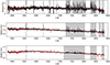 |
Fig. 1. Examples of different quality spectra with different S/N values. Shown is the relative flux on the y-axis and the wavelength on the x-axis (in angstroms). These spectra have not been shifted to the rest frame. The black line is the galaxy spectrum and the red line the fit produced by pPXF. The gray regions were manually masked out to improve the fit. From top to bottom are shown the spectra for the galaxies MATLAS-269, MATLAS-1232, and MATLAS-10 with S/N values of 8.7, 26.0, and 61.9, respectively. |
2.5. Full spectrum fitting
We fit the dwarf galaxy spectra using the Penalized Pixel-Fitting algorithm (pPXF; Cappellari & Emsellem 2004; Cappellari 2017), a standard full spectrum fitting method to extract stellar and gas kinematics as well as stellar populations. Employing a strategy similar to that used in the literature (e.g., Emsellem et al. 2019; Fensch et al. 2019; Müller et al. 2021b; Fahrion et al. 2022), we used single stellar population (SSP) models form the E-MILES library (Vazdekis et al. 2016) with ages ranging from 70 Myr to 14 Gyr and metallicites from solar down to −2.27 dex. We used a Kroupa initial mass function (IMF; Kroupa 2001) and accounted for the slightly varying MUSE resolution across the spectral range by convolving with a MUSE line spread function, as described in Guérou et al. (2017). In order to extract the line-of-sight velocities we used additive and multiplicative polynomials of degrees 8 and 12, respectively (Emsellem et al. 2019). For the stellar population properties of age and metallicity we fixed the determined velocity and rerun pPXF using only multiplicative polynomials of degree 12 (Fensch et al. 2019). In dwarf galaxies featuring emission lines, we determined the line-of-sight velocity by fitting absorption and emission lines simultaneously. For the stellar populations we first masked all emission lines, only leaving the absorption spectrum. We utilized the weights returned by pPXF to calculate the mean age and metallicity as well as the mass-to-light ratio (ML) in the V-band from the E-MILES SSPs for each galaxy. Here the ML is not a fitted parameter (such as age and metallicity), but is rather inferred from the age and metallicity grid returned by pPXF.
2.6. Signal-to-noise ratio optimization
The dwarf galaxies in this sample show a wide variety of S/N values. In Fig. 1 we show examples of different quality dwarf spectra (i.e., different S/N values). The black lines show the galaxy flux, while the red ones are the best-fit lines returned by pPXF. The gray regions were manually masked and were not considered in the fit. This can lead to curves in the fit line in these unconstrained regions. An example of this can be seen in the second and third spectra in Fig. 1 in the gray shaded region (∼7200–8000 Å). This does, however, not affect the quality of the fit.
In order to gain the maximum value from our MUSE data, we selected the aperture from which we extract the spectrum so that the S/N is optimized. To do this, we used the center of the dwarf galaxy and performed pPXF fitting for increasing aperture radii in a range r ∈ [10, 100] pix in steps of 10 pix. We chose this range based on the apparent sizes these dwarfs have in the MUSE image (∼300 × 300 pix). We used the aperture at the peak of the S/N to extract the spectrum and proceeded with the analysis. To illustrate the difference between the spectrum extracted using a visually intuited aperture and the S/N optimized one, we show the corresponding spectra for one of the dwarfs (MATLAS-445) in Fig. 2. As is done in other studies (e.g., Fahrion et al. 2019a, 2020; Müller et al. 2020, 2021b), we calculated the S/N in a region of the spectrum featuring no strong absorption or emission lines. Other works (e.g., Fahrion et al. 2019a; Müller et al. 2021b) have used the wavelength interval [6600,6800] Å for this purpose. Since the dwarf galaxies analyzed in this work show a range of different redshifts, we used this wavelength interval and shifted it using the estimated redshift for each galaxy via the best-fit recessional velocity. The S/N was calculated as the mean fraction between the flux and the square root of the variance. For this, the variance was multiplied by the χ2 value returned by pPXF, thus using a better estimate for the local noise (Fensch et al. 2019; Müller et al. 2020).
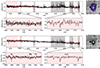 |
Fig. 2. Comparison of dwarf spectra from visually intuited aperture (top) vs. S/N optimized aperture (bottom). Right: stacked MUSE cube of the dwarf MATLAS-445. The spectra were extracted from the colored regions. The S/N was improved from 29.3 (visually intuited aperture) to 32.4 (optimized aperture) for this galaxy. |
For galaxies that are best described by an elliptical aperture, we increased the size by varying the semimajor axis a ∈ [10, 100] and keeping the axis ratio between minor and major axis of the ellipse constant. We used the radius or semimajor axis a for which the S/N peaks for all further analysis. In some instances the S/N does not show a peak in the tested interval but diverges. Individual inspection of these cases reveals that this only occurs in low S/N (≲10) and very faint galaxies. In these cases we manually set the aperture to best match visual intuition from the stacked data cube. It should be noted that for nucleated dwarfs we masked the nucleus for this S/N optimization in order to avoid a bias toward smaller apertures due to the nucleus dominating the S/N. We subsequently unmasked the nucleus when extracting the dwarf properties.
In the top panel of Fig. 3 we show the S/N distribution of all dwarfs in our sample, which takes values in the range ∼[5, 63]. In the bottom panel of the same figure we show the distribution of apertures (radius or semimajor axis), which lead to the maximum S/N for our dwarf sample, and relate these apertures to the effective radius from their GALFIT model (Habas et al. 2020; Poulain et al. 2021). We can see a prominent peak around ∼5 arcsec. In the top panel of Fig. 4 we see that the effective radius reff roughly traces the S/N optimized aperture, albeit with a rather large scatter, which increases significantly as the dwarf size increases. Since we obtained profiles describing the S/N as a function of the radius and have similar profiles of the surface brightness (measured in the g-band) as a function of the radius (see Poulain et al. 2021), we can relate the S/N with the surface brightness. In the bottom panel of Fig. 4 we show the distribution of the surface brightness at the S/N optimized dwarf radius. For eight dwarfs the S/N curve diverged and we set the optimal aperture manually at the first peak (if applicable) or based on visual intuition. We omitted these dwarfs from the plot. In a few cases we were not able to obtain the surface brightness profile from the MATLAS images directly, and measured it on the dwarf’s GALFIT model. These cases are shown in blue. We note a clear peak at ∼25.5 mag arcsec−2 and a second smaller one at ∼20 mag arcsec−2. Out of these 11 dwarfs in the lower peak, 8 show strong emission lines, which may explain the optimal radius at such high surface brightnesses. This distribution illustrates the gains expected in terms of S/N by probing deeper surface brightnesses.
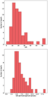 |
Fig. 3. Distributions of signal-to-noise ratios and corresponding optimized apertures from which the spectra were extracted. Top: distribution of S/N values for the sample of dwarf galaxies analyzed in this work. Bottom: distribution of S/N optimized apertures for the dwarf galaxies studied in this work. |
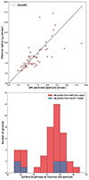 |
Fig. 4. Comparison of photometric properties with S/N optimized apertures. Top: comparison between S/N optimized radius from this work and the effective radius from Poulain et al. (2021). The black dashed line indicates the equality of the two measurements. Bottom: distribution of the dwarf g-band surface brightness from Poulain et al. (2021) at the radius that optimizes the S/N of the extracted spectrum. |
2.7. Error estimation
We estimated the errors for all properties by running a Monte Carlo (MC) simulation. We determined the best fit to the galaxy spectrum using pPXF and calculated the residuals between the best fit and input spectrum at each wavelength. We then created new realizations of the spectrum by using the best fit as a base line. At each wavelength we randomly added the residual or subtracted it from the best fit. We re-ran pPXF for the newly generated spectrum and compared the original values for the radial velocity, age, and metallicity with the returned values for the new realization. We repeated this 400 times for each galaxy. This number is motivated by the error estimation for the lowest S/N galaxy in our sample for which a recessional velocity is obtainable. We varied the number of MC runs in an interval NMC ∈ [100, 1000] in steps of 100 for this galaxy and observed stable values after 400 runs. The 1σ confidence interval of these MC simulations give the errors for each extracted property. We used the value of the initial best fit and calculated the errors in relation to the MC 1σ interval. If the best-fit value was outside of this interval (see Fig. 5), we used the mean and 1σ bounds of the MC simulation. In Appendix A we show the residuals of the best-fit value (velocity, age, and metallicity) minus the mean and median of the respective MC realizations and indicate whether the best-fit values lie within or outside the 1σ from the MC simulation. While overall the best-fit values are consistent with the mean and median of the MC realizations, there are some cases where the two values differ, in particular for the age.
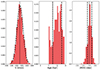 |
Fig. 5. Results from the MC error estimation with 400 iterations for the galaxy MATLAS-269. The histograms show the distributions of the fit values for the recessional velocity V, the age, and the metallicity obtained from pPXF by randomly flipping the sign of the residual between the galaxy spectrum and the initial best fit. The solid lines indicate the best-fit values of the original spectrum, while the dashed lines show the standard deviation of the MC realizations. For the recessional velocity shown in the leftmost panel, we fit a Gaussian curve (dashed line) to the distribution of MC realizations. |
3. Results and discussion
In the following we present the results of our analysis of the 56 noncluster dwarf galaxies and compare them against dwarfs in the literature. First, we discuss the line-of-sight velocities obtained from the MUSE spectra and relate this new information to the assumptions made in the MATLAS studies (e.g., Habas et al. 2020; Poulain et al. 2021, 2022; Marleau et al. 2021; Heesters et al. 2021). Next we illustrate the photometric properties of the subsample of MATLAS dwarfs observed with MUSE in relation to the MATLAS sample as a whole. We then examine the stellar population properties metallicity and age of this sample and compare them with dwarf properties from other works. We summarize the derived properties of the dwarf sample studied in this work in Table A.1.
3.1. Line-of-sight velocity
We obtain recessional velocity estimates from all but four galaxies in our sample (∼7%), for which the S/N is too low to identify or fit any spectral lines. The distribution of these velocities is shown in Fig. 6. The bulk of our sample (∼75%) shows velocities in an interval [1000, 3000] km s−1. This is consistent with the distance probed by the MATLAS survey of ∼10–45 Mpc with line-of-sight velocities ∈ [−300, 3800] km s−1. The dwarf galaxies in this velocity interval closely match the recessional velocities of nearby massive galaxies targeted in the ATLAS3D survey. The semi-automatic dwarf identification approach described in Habas et al. (2020) thus shows a success rate of 75% on this sample (79% for the dEs). We note that these numbers are lower limits for our dwarfs since the four dwarfs for which we could not obtain a velocity estimation may still be satellites of nearby host galaxies and were classified as nonsatellites for the sake of this calculation. We find that ten dwarf galaxies identified in the MATLAS fields, and previously assumed satellites of the respective targeted ETG in the field, show velocities that are inconsistent with any host in the distance range probed by ATLAS3D. These appear to lie farther in the background. We note that seven out of these ten galaxies show strong emission lines, indicating ongoing star formation. We expected this correlation since star forming objects appear brighter, and are thus detectable in our fields, whereas distant quiescent ones may largely be too faint, and thus elusive in this context. Another reason for this correlation is likely connected to the selection process of the MATLAS dwarfs during which a size cut was applied in order to remove background objects. Background dwarfs that remain in the sample after this cut are likely to be on the high end of the mass range and have a higher reservoir of gas and dust for star formation. Furthermore, star forming objects are challenging to classify and distance estimation based on visual intuition through surface brightness fluctuation is inapplicable for such objects.
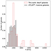 |
Fig. 6. Distribution of measured dwarf line-of-sight velocities studied in this work. The first peak corresponds to the velocity space, which is consistent with the hosts targeted in the ATLAS3D survey. |
We matched the dwarf recessional velocities with the one of nearby ATLAS3D host galaxies and declared them satellites of the host with the smallest velocity difference ΔV = Vsat − Vhost. We find a maximum ΔVmax = 460 km s−1 and a maximum projected separation between host and satellite of Δdmax = 391 kpc. There is a clear gap in the velocity distribution shown in Fig. 6 between the dwarfs matching the hosts in the probed MATLAS distance range (first peak) and the background dwarfs. We reassign the dwarfs from the assumed host in the MATLAS studies (targeted ETG in each field) to new hosts according to their best ΔV match and show the results of this procedure in Fig. 7. We plot the projected distance between satellite and host in kiloparsec on the x-axis and the difference in recessional velocities on the y-axis. The gray circles indicate the values following the MATLAS assumptions, which are shifted toward the red points (black arrows) by assigning a better matching host galaxy with the new spectral information. For the red points circled in gray the assumed MATLAS host does not change with new velocity information. We indicate the ±300 km s−1 boundaries as dashed lines, which is a typical relative velocity cut for satellite populations. This is, however, not a strict cutoff as greater velocity dispersions are possible in group environments. If we instead adopt a cut of ΔV ∼ 500 km s−1, as is done in Habas et al. (2020), all of our matched dwarfs lie within.
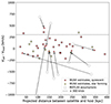 |
Fig. 7. Projected distance between satellite and assumed host galaxy in kpc vs. recessional velocity difference between satellite and host (ΔV = Vsat − Vhost) in km s−1. The projected distance and velocity difference to the host assumed in MATLAS are plotted (gray circles) compared with the updated host based on minimal ΔV through MUSE spectral fitting (red points). These shifts are indicated by black arrows. For the red points circled in gray the assumed host stays the same with new velocity information on the dwarf. The dashed black lines show ±300 km s−1. |
3.2. Photometric properties
In order to illustrate whether our MATLAS subsample with MUSE observations is representative of the MATLAS sample overall, we compare their photometric properties from the GALFIT (Peng et al. 2002, 2010) modeling (see Habas et al. 2020; Poulain et al. 2021) in Fig. 8. We show the Sersic index, the g-band apparent magnitude mg, the effective radius reff in arcsec, and the axis ratio. The MATLAS sample consisting of 1589 dwarfs with successful GALFIT models and reliable reff estimates is shown in gray; the subsample with MUSE observations is in red. Both samples are displayed normalized for improved visibility. The samples overlap well in general. We note a shift toward brighter magnitudes and larger effective radii for the MUSE sample. This is caused by our observational selection criteria, which are in place to ensure sufficient S/N for our main objectives in a single OB. We note that there are no ultra-diffuse galaxies (UDGs; i.e., dwarfs with excess effective radius) in our MUSE sample.
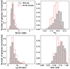 |
Fig. 8. Photometric properties of MATLAS subsample targeted with MUSE (red) and overall distribution of the MATLAS dwarf galaxies (gray) with robust GALFIT modeling. Top left: Sersic index; top right: apparent g-band magnitude mg; bottom left: effective radius reff; bottom right: axis ratio. |
We show the scaling relation absolute magnitude Mg versus effective radius reff in Fig. 9 (see also Habas et al. 2020; Poulain et al. 2021, 2022; Marleau et al. 2021). Since there are no distance or velocity estimates for the majority of the MATLAS dwarfs, Mg was estimated by assuming the distance of central ETG of the field the dwarf appears in. Some of the dwarf galaxies (≈15%) have a distance or velocity estimate from other surveys, in which case we use this estimate. For the MUSE sample we use the distance of the massive galaxy which best matches the MUSE estimate in terms of line-of-sight velocity. These host distances are taken from the ATLAS3D survey and are mostly based on redshift and surface brightness fluctuation (SBF) measurements (see Cappellari et al. 2011a). For dwarfs that are not satellites of any host in the ATLAS3D catalog, we use the recessional velocity obtained via MUSE spectroscopy and transform it into the distance space via Hubble’s law D = V/H0. Here D denotes the distance to the dwarf, v the line-of-sight velocity, and H0 the Hubble constant (H0 = (69.8 ± 1.7) km s−1 Mpc−1; Freedman 2021). There is no notable difference between the subsample with MUSE observations (red) and the full MATLAS sample (gray) with GALFIT models. We therefore conclude that our MUSE sample is representative of the dwarf galaxies identified in the MATLAS survey.
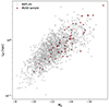 |
Fig. 9. Scaling relation absolute g-band magnitude Mg vs. effective radius reff in kpc. Comparison between the dwarf sample studied in this work (red) and the overall MATLAS sample (gray). To get these measurements for the sample with MUSE observations, the associated host galaxy is used to estimate the distance; if not available, the dwarf velocity via Hubble’s law is used. |
3.3. Stellar populations
Dwarf galaxies in the Local Universe follow the universal stellar mass-metallicity relation (Kirby et al. 2013). In order to relate our data to this observation, we estimate the stellar mass M* of our dwarf galaxies by first transforming the apparent g-band magnitude mg from Poulain et al. (2021) to the V-band by using the transformation equation from Lupton (2005),
 (1)
(1)
and use the g–r colors from Poulain et al. (2021). For the galaxies without g–r values from GALFIT we use the g–r estimates from Source Extractor on the MATLAS images by using an aperture of 3reff. We then transform the apparent V-band magnitude to the absolute magnitude MV. For this we estimate the distance to the dwarf galaxy as described in Sect. 3.2. Finally, we convert the absolute magnitude MV to LV and use the stellar mass-to-light estimate from pPXF to estimate the stellar mass M*.
In Fig. 10 we present the results from our sample (red) and compare it with the relation shown in Kirby et al. (2013) and data points from other works. It should be noted that we show all LG dwarfs listed in Table 4 of Kirby et al. (2013). The presented fit, however, excludes the M31 dwarfs, since a different technique (coadded spectra) was used to estimate the metallicities and their uncertainties are larger when compared to the Milky Way (MW) dwarfs. We note that our dwarf sample shows a wide range of different S/N values (see Fig. 3). In order to gain robust estimates on the stellar populations high S/N values are needed (see Fig. A.1. in Fahrion et al. 2019b). We are not able to reach high values for all galaxies but distinguish our results accordingly (see Fig. 10, left vs. right).
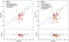 |
Fig. 10. Plot of universal stellar mass-metallicity relation from Kirby et al. (2013; blue solid line) with its rms (blue dashed lines). On the x-axis is plotted the logarithm of the stellar mass in units of solar mass. Left: data from this work (red circles), but excluding star forming and low S/N galaxies. Right: full sample from this work. Star forming galaxies are shown as yellow upward pointing triangles, while low S/N galaxies are gray downward pointing triangles. Shown is a comparison of our results with galaxies from other works: LG dwarfs (blue; Kirby et al. 2013), Cen A dwarfs (pink; Müller et al. 2021b), galaxies in Fornax and Virgo (green; Fahrion et al. 2021), nucleated dwarf LTGs (purple; Fahrion et al. 2022), and UDGs in the Coma cluster (orange; Chilingarian et al. 2019). Bottom: residual plots (i.e., metallicity dwarf-metallicity fit). The blue dashed lines indicate the rms of the fit from Kirby et al. (2013). The LG dwarf metallicities from Kirby et al. (2013) are iron metallicities ([Fe/H]), while all other data points show total metallicities ([M/H]). |
In the left plot in Fig. 10 we show only quiescent dwarf galaxies, and exclude cases with low S/N (≲ 8) spectra. In the right plot, we show the full sample, including star forming galaxies (yellow) and galaxies with low S/N spectra (gray). As discussed in Sect. 2.5, we masked all emission lines in star forming galaxies to determine the stellar population properties age and metallicity. This leaves only the calcium triplet (CaT) for the estimation of these properties. Since the S/N in the remaining absorption spectrum is not high enough to make robust estimates, we treat these cases separately and note reduced reliability. For all but one of the galaxies with low S/N values (gray) the metallicity estimation is on the lower end of the possible values from the considered SSPs. For these cases we cannot derive meaningful results.
We see a systematic shift to lower metallicites in our sample compared with the LG dwarf galaxies. This shift is consistent with observations in other works, Fahrion et al. (2021, Fornax & Virgo galaxies, and 2022, nucleated dwarf LTGs), for this stellar mass range. As mentioned in Sect. 1, however, this shift may be attributed to different strategies of measuring the metallicities between Kirby et al. (2013), this work, and the other works cited in this study. Kirby et al. (2013) perform spectroscopy on individual RGB stars in order to obtain the metallicity, whereas we and other studies used for comparison (Fahrion et al. 2021, 2022; Müller et al. 2021b; Chilingarian et al. 2019) measure the metallicity with full spectrum fitting. We are thus sensitive to the entire stellar population properties, whereas Kirby et al. (2013) present the mean metallicity over the RGB population in each galaxy. Another factor to consider is that the metallicities from Kirby et al. (2013) are based on the iron absorption lines (Fe I), while we use lines across the entire spectral range probed by MUSE (including Hβ, Hα, the Mg Triplet, Fe I, the Ca Triplet). The E-MILES “base” models we are using assume that the integrated metallicity [M/H] is equal to the iron metallicity [Fe/H]. This assumption, however, only holds true at high metallicities (≳ − 1 dex). Low-metallicity stars, which are abundant in our dwarf galaxies, are alpha-enhanced, which boosts [M/H] compared to [Fe/H]. Considering this assumption, the [Fe/H] as measured in Kirby et al. (2013) should be lower than the [M/H] in our dwarf sample, which would make the discrepancy even stronger. We find that the S/N in our sample is too low to estimate [Fe/H] directly via line index measurements (Vazdekis et al. 2010) or to determine [Mg/Fe] as an additional fit parameter, which would help bridge the difference in the two measurement methods for the metallicity.
Boecker et al. (2020) use MUSE to compare age and metallicity measurements from individual stars and full spectrum fitting for the nuclear star cluster (NSC) M54. Interestingly, they find that the two methods show excellent agreement, and note only a 3% difference in age and 0.2 dex in metallicity. The values for full spectrum fitting suggest older and more metal poor stellar populations when compared to the integrated spectra from individual stars. The study finds a metal poor and a metal rich component in the NSC. The two methods are consistent on the low-metallicity component, while full spectrum fitting returns a higher metallicity estimate for the high-metallicity component. Similar to our study, the authors discuss alpha-abundances and find that alpha-enhancement in metal poor stars cannot explain the difference in these measurements since the exact opposite behavior would be expected in this context.
Below the mass-metallicity plots in Fig. 10, we show the residual (i.e., the difference between the Kirby et al. (2013) relation and the data points). The gray dotted lines show the rms from Kirby et al. (2013). The systematic shift toward lower metallicities with the exception of three galaxies is even more apparent in this plot. A two-sample Kolmogorov–Smirnov (KS) test comparing the residual values for the LG dwarfs from Kirby et al. (2013) and the residuals from the clean sample (quiescent, medium to high S/N) in this work, reveals a p-value of p = 0.002. This indicates that the two samples show significant differences. While there is a significant scatter in other works (most notably Chilingarian et al. 2019), it is interesting that all but three galaxies in our sample show on average lower metallicity values than the MW dwarfs.
In order to test whether the insufficient S/N in some of our dwarf spectra could be a contributing factor in the discrepancy between Kirby et al. (2013) and this study, we deteriorated the quality of our highest S/N dwarf spectrum (MATLAS-553). To do this we first determined the best fit via pPXF and calculated the residuals between the best fit and the input galaxy spectrum at each wavelength. We then multiplied the residuals with values from a Gaussian distribution with mean 0 and standard deviation σ and added the products back to the best fit at every wavelength. We then ran pPXF on this newly generated spectrum and noted the returned metallicity. In order to increase the statistical significance of this test, we created 100 realizations for a range of σ ∈ [2, 8] in steps of one. A higher value for σ leads to a higher degree of S/N deterioration compared to the original spectrum. In Fig. 11 we present the results of this test, which shows the mean metallicity from 100 realizations as a function of σ. The error bars show the standard deviation of the MC metallicity distributions. As we would expect, the errors increase as the S/N becomes lower. If the low S/N in our sample would push the metallicity estimates toward lower values, we would expect a decreasing trend in this plot. Since we note no obvious behavior in that regard, we can rule out the S/N in our sample as a leading factor in the observed offset.
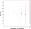 |
Fig. 11. Mean metallicity as a function of different degrees of spectrum deterioration for the highest S/N dwarf in the sample (MATLAS-553; S/N ∼ 62). The error bars on the y-axis show the standard deviation of 100 MC realizations for every σ. The best-fit value for the metallicity is −1.29 dex. |
Considering the results from Boecker et al. (2020), the offset in the quiescent medium to high S/N dwarfs is fully mitigated by shifting the entire sample by 0.2 dex toward higher metallicities. A two-sample KS test yields a p-value of pshift = 0.8928 after this shift, suggesting that the two samples are consistent with following the same distribution. If we add the star forming galaxies to this test (low S/N galaxies excluded), however, the offset is still statistically significant with a KS p-value of pshift all = 0.0432.
Another factor that could contribute to the offset in metallicities is the different environments in which the dwarf galaxies reside. We tested this hypothesis by investigating the local density as described in Cappellari et al. (2011b) as a function of the residuals between the relation presented in Kirby et al. (2013) and the values from this study. The local density parameter
 (2)
(2)
is defined as the ten nearest massive galaxies Ngal of the assumed host galaxy divided by the sphere of radius r10 which encloses these ten neighbors. In Habas et al. (2020) a correlation between this parameter and the morphology of the MATLAS dwarfs is found. We used the dwarf galaxies in our sample for which we could find a matching host in the ATLAS3D survey volume and compared its ρ10 measure with the metallicity offset from the MZR. We show the results of this test in Fig. 12. Quiescent dwarfs are shown as red circles and star forming ones as yellow triangles. We see no apparent trend, and can therefore not attribute the offset to the different density environments.
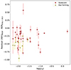 |
Fig. 12. Residuals between metallicities for our dwarfs and the MZR from Kirby et al. (2013) as a function of the local density parameter ρ10. |
Finally, we tested whether the nucleus has any influence on the metallicity estimate, and compare our results if we mask the nucleus or extract the spectra from the entire galaxy. We find very small differences between extracted metallicities with shifts in no particular direction. On average we find a difference of 0.002 dex toward lower metallicities with masked nuclei. For the dENs in our sample, the nucleus therefore does not contribute to the observed systematic offset.
In Fig. 13 we show our results of the estimated age (in Gyr) versus the metallicity of our dwarf sample and compare them with results from other works. It is important to note the large error bars for the age estimates, showing the difficulty of constraining this property with the quality type of spectra at hand. Overall we report an average old (6–14 Gyr) and metal poor (−1.9 to −1.3 dex) stellar population for most of these dwarf galaxies with a few outliers at the upper and lower end for the metallicity. We once again compare our sample with other works: galaxies in the Fornax and Virgo clusters are shown in green (Fahrion et al. 2021), nucleated dwarf LTGs in purple (Fahrion et al. 2022), the dwarf galaxies around Centaurus A in pink (Müller et al. 2021b), and UDGs in the Coma cluster in orange (Chilingarian et al. 2019). Even though the measurement errors are rather large, we can see that our sample is concentrated in the lower right corner of Fig. 13, comparable with the Cen A dwarfs (Müller et al. 2021b). Cluster dwarfs and nucleated dwarf LTGs appear to span a larger range of ages in comparison.
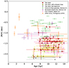 |
Fig. 13. Age vs. metallicity. The dwarf galaxies presented in this work are shown as red circles, yellow upward pointing triangles (star forming), and gray downward pointing triangles (low-quality spectra). Shown is a comparison with the results from other studies: galaxies in the Fornax and Virgo clusters (green; Fahrion et al. 2021), nucleated dwarf LTGs (purple; Fahrion et al. 2022), Cen A dwarfs (pink; Müller et al. 2021b), and UDGs in the Coma cluster (orange; Chilingarian et al. 2019). |
4. Conclusions
In this work we analyzed 56 dwarf galaxies based on MUSE spectroscopic observations. These galaxies are part of a large sample of dwarfs that had been previously identified in the MATLAS low- to moderate-density fields beyond the Local Volume. Through comparison with the overall photometric properties of the MATLAS dwarf sample, we find that our subsample observed with MUSE is representative of the dwarfs identified in MATLAS. Through full spectrum fitting with pPXF, we retrieved their line-of-sight velocity and stellar population properties age and metallicity. Our main results are the following:
-
The bulk of the 56 dwarfs (42, or 75%) show line-of-sight velocities that match the velocities of massive ATLAS3D galaxies in the field: ∼1000–3000 km s−1. This increases to 79% for dEs. Almost one-third (∼30%) of the dwarf galaxies in the ATLAS3D velocity range show star forming activity. Based on the minimal velocity difference ΔV between massive and dwarf galaxy, we determine the satellite membership of the dwarf galaxies in our sample. We updated the previously assumed association in Fig. 7 and conclude that our assumption (that dwarfs are associated with the central targeted ETG in each field) is correct in 57% of the cases for the presented sample.
-
We find that ∼18% (10) of the dwarfs in this sample are located farther in the background, outside of the ATLAS3D survey volume. Of these ten dwarfs, 70% show emission lines, which is not unexpected in light of the semi-automatic identification approach for the MATLAS dwarfs (see Habas et al. 2020). There are no spectral lines apparent for 7% (4) of the dwarfs in this sample, thus we cannot extract any velocity information.
-
We demonstrate the viability of the MUSE instrument for the study of low surface brightness dwarf galaxies in filler conditions and with a single observational block per galaxy. We determined the radius that optimizes the S/N of the extracted spectrum for each galaxy and related it to the surface brightness in Fig. 4. The distribution of surface brightnesses at the optimized radius illustrates that there are significant gains in probing to a depth of ∼27 mag arcsec−2, but diminishing returns in terms of S/N thereafter.
-
We find that the dwarfs presented in this work deviate from the universal stellar mass-metallicity relation shown in Kirby et al. (2013). The bulk of our sample is systematically offset toward lower metallicities, a property which, in this stellar mass range, can also be seen in dwarfs analyzed in other works. While the bulk of the sample with stellar masses in the range 106.5–108.5M*/M⊙ is more metal poor than the LG dwarfs, only the two dwarfs with the highest stellar mass agree well with the universal mass-metallicity relation. We note that the star forming dwarfs in particular show a greater offset when compared to the quiescent ones. This could be due to the fact that only the CaT is left for this estimation since all other lines show emissions and are therefore masked. The CaT may be insufficient to obtain a robust metallicity measurement.
-
The overall shift toward lower metallicities at a given stellar mass cannot be attributed to insufficient S/N values in our dwarf spectra nor to the different density environments the dwarf galaxies reside in.
-
We compare the age versus metallicity of the dwarfs presented in this work with the results from other comparable studies in Fig. 13. Although the error bars on the age are quite large, we can say that our sample is old (6–14 Gyr) and mostly metal poor (−1.9 to −1.3 dex), which is consistent with the Centaurus A satellites (Müller et al. 2021b). Dwarfs located in clusters are more metal rich and span a wider range of ages (Chilingarian et al. 2019; Fahrion et al. 2021).
Our results suggest that there may be a systematic deviation from the LG stellar mass-metallicity relation. However, this deviation may be due to the difference in methodologies for deriving metallicities. Kirby et al. (2013) base their results on individual RGB stars, while we use full spectrum fitting, as do other works. Boecker et al. (2020) find a measurement shift of 0.2 dex toward lower metallicities for full spectrum fitting when compared to the resolved stellar population analysis. By applying this shift toward higher metallicities, the offset is fully mitigated for the quiescent dwarfs, but remains when also considering star forming dwarfs. However, this measurement difference is based on the analysis of a single object, and therefore does not hold statistical significance. In order to be able to paint a clearer picture of this matter, more methodology comparisons such as Boecker et al. (2020) are needed. In addition, more high-quality spectra of dwarfs, particularly in the mass domain between the dwarf and massive galaxy regime, will help clarify whether the offset only occurs for dwarfs below a certain stellar mass threshold since our highest mass galaxies, as well as high-mass galaxies from other works, are consistent with the MZR. From our results it is plausible that full spectrum fitting of dwarf galaxies may lead to a steeper slope for the MZR or even a nonlinear relation.
Acknowledgments
We thank the referee for the constructive report, which helped to clarify and improve the manuscript. N.H. and O.M. are grateful to the Swiss National Science Foundation for financial support under the grant number PZ00P2_202104. M.P. is supported by the Academy of Finland grant no: 347089. S.L. acknowledges the support from the Sejong Science Fellowship Program by the National Research Foundation of Korea (NRF) grand funded by the Korea goverment (MSIT) (No. NRF-2021R1C1C2006790). N.H. and O.M. thank Guisseppina Battaglia for pointing out the work by Boecker et al. (2020). We thank the International Space Science Institute (ISSI) in Bern (Switzerland) for hosting our international team for a workshop on “Space Observations of Dwarf Galaxies from Deep Large Scale Surveys: The MATLAS Experience”.
References
- Andrews, B. H., & Martini, P. 2013, ApJ, 765, 140 [NASA ADS] [CrossRef] [Google Scholar]
- Bacon, R., Accardo, M., Adjali, L., et al. 2010, Proc. SPIE, 7735, 131 [Google Scholar]
- Bacon, R., Accardo, M., Adjali, L., et al. 2012, The Messenger, 147, 4 [NASA ADS] [Google Scholar]
- Bell, E. F., Slater, C. T., & Martin, N. F. 2011, ApJ, 742, L15 [NASA ADS] [CrossRef] [Google Scholar]
- Bennet, P., Sand, D., Crnojević, D., et al. 2017, ApJ, 850, 109 [NASA ADS] [CrossRef] [Google Scholar]
- Bennet, P., Sand, D., Crnojević, D., et al. 2019, ApJ, 885, 153 [NASA ADS] [CrossRef] [Google Scholar]
- Bennet, P., Sand, D. J., Crnojević, D., et al. 2020, ApJ, 893, L9 [CrossRef] [Google Scholar]
- Bertin, E., & Arnouts, S. 1996, A&AS, 117, 393 [NASA ADS] [CrossRef] [EDP Sciences] [Google Scholar]
- Bílek, M., Duc, P.-A., Cuillandre, J.-C., et al. 2020, MNRAS, 498, 2138 [Google Scholar]
- Binggeli, B., & Jerjen, H. 1997, in Galaxy Scaling Relations: Origins, Evolution and Applications: Proceedings of the ESO Workshop Held at Garching, Germany, 18–20 November 1996 (Springer), 103 [Google Scholar]
- Binggeli, B., Tarenghi, M., & Sandage, A. 1990, A&A, 228, 42 [NASA ADS] [Google Scholar]
- Boecker, A., Alfaro-Cuello, M., Neumayer, N., Martín-Navarro, I., & Leaman, R. 2020, ApJ, 896, 13 [NASA ADS] [CrossRef] [Google Scholar]
- Brook, C., Stinson, G., Gibson, B. K., et al. 2014, MNRAS, 443, 3809 [NASA ADS] [CrossRef] [Google Scholar]
- Brooks, A. M., Governato, F., Booth, C., et al. 2007, ApJ, 655, L17 [NASA ADS] [CrossRef] [Google Scholar]
- Bullock, J. S., & Boylan-Kolchin, M. 2017, ARA&A, 55, 343 [Google Scholar]
- Buonanno, R., Corsi, C., Fusi Pecci, F., Hardy, E., & Zinn, R. 1985, A&A, 152, 65 [NASA ADS] [Google Scholar]
- Cappellari, M. 2017, MNRAS, 466, 798 [Google Scholar]
- Cappellari, M., & Emsellem, E. 2004, PASP, 116, 138 [Google Scholar]
- Cappellari, M., Bacon, R., Bureau, M., et al. 2006, MNRAS, 366, 1126 [Google Scholar]
- Cappellari, M., Emsellem, E., Krajnović, D., et al. 2011a, MNRAS, 413, 813 [Google Scholar]
- Cappellari, M., Emsellem, E., Krajnović, D., et al. 2011b, MNRAS, 416, 1680 [Google Scholar]
- Carlsten, S. G., Beaton, R. L., Greco, J. P., & Greene, J. E. 2019, ApJ, 878, L16 [NASA ADS] [CrossRef] [Google Scholar]
- Carlsten, S. G., Greene, J. E., Beaton, R. L., Danieli, S., & Greco, J. P. 2022, ApJ, 933, 47 [CrossRef] [Google Scholar]
- Chiboucas, K., Jacobs, B. A., Tully, R. B., & Karachentsev, I. D. 2013, AJ, 146, 126 [Google Scholar]
- Chilingarian, I. V., Afanasiev, A. V., Grishin, K. A., Fabricant, D., & Moran, S. 2019, ApJ, 884, 79 [NASA ADS] [CrossRef] [Google Scholar]
- Chiosi, C., D’Onofrio, M., Merlin, E., Piovan, L., & Marziani, P. 2020, A&A, 643, A136 [NASA ADS] [CrossRef] [EDP Sciences] [Google Scholar]
- Cohen, Y., van Dokkum, P., Danieli, S., et al. 2018, ApJ, 868, 96 [Google Scholar]
- Courteau, S., Dutton, A. A., van den Bosch, F. C., et al. 2007, ApJ, 671, 203 [Google Scholar]
- Cowie, L. L., Songaila, A., Hu, E. M., & Cohen, J. 1996, AJ, 112, 839 [NASA ADS] [CrossRef] [Google Scholar]
- Crnojević, D., Sand, D. J., Bennet, P., et al. 2019, ApJ, 872, 80 [Google Scholar]
- Danieli, S., van Dokkum, P., Merritt, A., et al. 2017, ApJ, 837, 136 [NASA ADS] [CrossRef] [Google Scholar]
- Danieli, S., van Dokkum, P., Trujillo-Gomez, S., et al. 2022, ApJ, 927, L28 [NASA ADS] [CrossRef] [Google Scholar]
- Davis, A. B., Nierenberg, A. M., Peter, A. H. G., et al. 2021, MNRAS, 500, 3854 [Google Scholar]
- Djorgovski, S., & Davis, M. 1987, ApJ, 313, 59 [Google Scholar]
- D’Onofrio, M., Marziani, P., & Chiosi, C. 2021, Front. Astron. Space Sci., 8, 157 [Google Scholar]
- Dressler, A., Lynden-Bell, D., Burstein, D., et al. 1987, ApJ, 313, 42 [Google Scholar]
- Drlica-Wagner, A., Bechtol, K., Mau, S., et al. 2020, ApJ, 893, 47 [CrossRef] [Google Scholar]
- Drlica-Wagner, A., Carlin, J. L., Nidever, D. L., et al. 2021, ApJS, 256, 2 [NASA ADS] [CrossRef] [Google Scholar]
- Duc, P.-A., Cuillandre, J.-C., Karabal, E., et al. 2015, MNRAS, 446, 120 [Google Scholar]
- Eigenthaler, P., Puzia, T. H., Taylor, M. A., et al. 2018, ApJ, 855, 142 [Google Scholar]
- Emsellem, E., van der Burg, R. F. J., Fensch, J., et al. 2019, A&A, 625, A76 [NASA ADS] [CrossRef] [EDP Sciences] [Google Scholar]
- Erb, D. K., Steidel, C. C., Shapley, A. E., et al. 2006, ApJ, 646, 107 [NASA ADS] [CrossRef] [Google Scholar]
- Faber, S., & Jackson, R. E. 1976, ApJ, 204, 668 [NASA ADS] [CrossRef] [Google Scholar]
- Fahrion, K., Georgiev, I., Hilker, M., et al. 2019a, A&A, 625, A50 [NASA ADS] [CrossRef] [EDP Sciences] [Google Scholar]
- Fahrion, K., Lyubenova, M., van de Ven, G., et al. 2019b, A&A, 628, A92 [NASA ADS] [CrossRef] [EDP Sciences] [Google Scholar]
- Fahrion, K., Müller, O., Rejkuba, M., et al. 2020, A&A, 634, A53 [NASA ADS] [CrossRef] [EDP Sciences] [Google Scholar]
- Fahrion, K., Lyubenova, M., van de Ven, G., et al. 2021, A&A, 650, A137 [NASA ADS] [CrossRef] [EDP Sciences] [Google Scholar]
- Fahrion, K., Bulichi, T.-E., Hilker, M., et al. 2022, A&A, 667, A101 [NASA ADS] [CrossRef] [EDP Sciences] [Google Scholar]
- Fensch, J., van der Burg, R. F. J., Jeřábková, T., et al. 2019, A&A, 625, A77 [NASA ADS] [CrossRef] [EDP Sciences] [Google Scholar]
- Ferguson, H. C., & Binggeli, B. 1994, A&ARv, 6, 67 [NASA ADS] [CrossRef] [Google Scholar]
- Ferguson, H. C., & Sandage, A. 1989, ApJ, 346, L53 [NASA ADS] [CrossRef] [Google Scholar]
- Ferguson, H., Sandage, A., Hollenbach, D., & Thronson Harley, A. J. 1990, NASA Conference Publication (Washington, DC: National Aeronautics and Space Administration), 3084 [Google Scholar]
- Ferrarese, L., Cote, P., Cuillandre, J.-C., et al. 2012, ApJS, 200, 4 [NASA ADS] [CrossRef] [Google Scholar]
- Fitzpatrick, P. J., & Graves, G. J. 2015, MNRAS, 447, 1383 [NASA ADS] [CrossRef] [Google Scholar]
- Font, A. S., Benson, A. J., Bower, R. G., et al. 2011, MNRAS, 417, 1260 [NASA ADS] [CrossRef] [Google Scholar]
- Freedman, W. L. 2021, ApJ, 919, 16 [NASA ADS] [CrossRef] [Google Scholar]
- Frenk, C. S., & White, S. D. M. 2012, Ann. Phys., 524, 507 [NASA ADS] [CrossRef] [Google Scholar]
- Gallazzi, A., Charlot, S., Brinchmann, J., White, S. D. M., & Tremonti, C. A. 2005, MNRAS, 362, 41 [Google Scholar]
- Gallazzi, A., Charlot, S., Brinchmann, J., & White, S. D. M. 2006, MNRAS, 370, 1106 [Google Scholar]
- Garnett, D. R. 2002, ApJ, 581, 1019 [NASA ADS] [CrossRef] [Google Scholar]
- Geha, M., Wechsler, R. H., Mao, Y.-Y., et al. 2017, ApJ, 847, 4 [NASA ADS] [CrossRef] [Google Scholar]
- González Delgado, R. M., Cid Fernandes, R., García-Benito, R., et al. 2014, ApJ, 791, L16 [CrossRef] [Google Scholar]
- Greco, J. P., Greene, J. E., Strauss, M. A., et al. 2018, ApJ, 857, 104 [NASA ADS] [CrossRef] [Google Scholar]
- Guérou, A., Krajnović, D., Epinat, B., et al. 2017, A&A, 608, A5 [Google Scholar]
- Habas, R., Marleau, F. R., Duc, P.-A., et al. 2020, MNRAS, 491, 1901 [NASA ADS] [Google Scholar]
- Heesters, N., Habas, R., Marleau, F. R., et al. 2021, A&A, 654, A161 [NASA ADS] [CrossRef] [EDP Sciences] [Google Scholar]
- Hou, J., Yu, Q., & Lu, Y. 2014, ApJ, 791, 8 [NASA ADS] [CrossRef] [Google Scholar]
- Ibata, R., Martin, N. F., Irwin, M., et al. 2007, ApJ, 671, 1591 [CrossRef] [Google Scholar]
- Ibata, R. A., Lewis, G. F., Conn, A. R., et al. 2013, Nature, 493, 62 [NASA ADS] [CrossRef] [Google Scholar]
- Ibata, R. A., Lewis, G. F., McConnachie, A. W., et al. 2014, ApJ, 780, 128 [Google Scholar]
- Irwin, J. A., Hoffman, G. L., Spekkens, K., et al. 2009, ApJ, 692, 1447 [NASA ADS] [CrossRef] [Google Scholar]
- Kewley, L. J., & Ellison, S. L. 2008, ApJ, 681, 1183 [Google Scholar]
- Kim, E., Kim, M., Hwang, N., et al. 2011, MNRAS, 412, 1881 [NASA ADS] [CrossRef] [Google Scholar]
- Kim, S. Y., Peter, A. H. G., & Hargis, J. R. 2018, Phys. Rev. Lett., 121, 211302 [CrossRef] [Google Scholar]
- Kirby, E. N., Cohen, J. G., Guhathakurta, P., et al. 2013, ApJ, 779, 102 [Google Scholar]
- Koposov, S., Belokurov, V., Evans, N. W., et al. 2008, ApJ, 686, 279 [NASA ADS] [CrossRef] [Google Scholar]
- Köppen, J., Weidner, C., & Kroupa, P. 2007, MNRAS, 375, 673 [CrossRef] [Google Scholar]
- Kormendy, J. 1977, ApJ, 218, 333 [NASA ADS] [CrossRef] [Google Scholar]
- Kroupa, P. 2001, MNRAS, 322, 231 [NASA ADS] [CrossRef] [Google Scholar]
- Kunkel, W. E., & Demers, S. 1976, IAU Symp., 182, 241 [NASA ADS] [Google Scholar]
- Kuntschner, H., Lucey, J. R., Smith, R. J., Hudson, M. J., & Davies, R. L. 2001, MNRAS, 323, 615 [NASA ADS] [CrossRef] [Google Scholar]
- La Barbera, F., Busarello, G., Merluzzi, P., et al. 2008, ApJ, 689, 913 [NASA ADS] [CrossRef] [Google Scholar]
- La Marca, A., Peletier, R., Iodice, E., et al. 2022, A&A, 659, A92 [NASA ADS] [CrossRef] [EDP Sciences] [Google Scholar]
- Lee, H., Skillman, E. D., Cannon, J. M., et al. 2006, ApJ, 647, 970 [NASA ADS] [CrossRef] [Google Scholar]
- Lequeux, J., Peimbert, M., Rayo, J., Serrano, A., & Torres-Peimbert, S. 1979, A&A, 80, 155 [NASA ADS] [Google Scholar]
- Li, Y.-S., De Lucia, G., & Helmi, A. 2010, MNRAS, 401, 2036 [NASA ADS] [CrossRef] [Google Scholar]
- Lian, J., Thomas, D., & Maraston, C. 2018, MNRAS, 481, 4000 [Google Scholar]
- Lu, Y., Wechsler, R. H., Somerville, R. S., et al. 2014, ApJ, 795, 123 [CrossRef] [Google Scholar]
- Lu, Y., Benson, A., Wetzel, A., et al. 2017, ApJ, 846, 66 [NASA ADS] [CrossRef] [Google Scholar]
- Lupton, R. 2005, Transformations between SDSS magnitudes and other systems, https://www.sdss3.org/dr10/algorithms/sdssUBVRITransform.php/ [Google Scholar]
- Lynden-Bell, D. 1976, MNRAS, 174, 695 [NASA ADS] [Google Scholar]
- Ma, X., Hopkins, P. F., Faucher-Giguère, C.-A., et al. 2016, MNRAS, 456, 2140 [NASA ADS] [CrossRef] [Google Scholar]
- Magorrian, J., Tremaine, S., Richstone, D., et al. 1998, AJ, 115, 2285 [Google Scholar]
- Maiolino, R., & Mannucci, F. 2019, A&ARv, 27, 3 [Google Scholar]
- Mannucci, F., Cresci, G., Maiolino, R., Marconi, A., & Gnerucci, A. 2010, MNRAS, 408, 2115 [NASA ADS] [CrossRef] [Google Scholar]
- Mao, Y.-Y., Geha, M., Wechsler, R. H., et al. 2021, ApJ, 907, 85 [NASA ADS] [CrossRef] [Google Scholar]
- Marleau, F. R., Habas, R., Poulain, M., et al. 2021, A&A, 654, A105 [NASA ADS] [CrossRef] [EDP Sciences] [Google Scholar]
- Martin, N. F., Ibata, R. A., Irwin, M. J., et al. 2006, MNRAS, 371, 1983 [NASA ADS] [CrossRef] [Google Scholar]
- Martin, N. F., Ibata, R. A., Lewis, G. F., et al. 2016, ApJ, 833, 167 [NASA ADS] [CrossRef] [Google Scholar]
- Mateo, M. L. 1998, ARA&A, 36, 435 [NASA ADS] [CrossRef] [Google Scholar]
- McClure, R. D., & van den Bergh, S. 1968, AJ, 73, 1008 [NASA ADS] [CrossRef] [Google Scholar]
- McConnachie, A. W. 2012, AJ, 144, 4 [Google Scholar]
- McConnachie, A. W., Irwin, M. J., Ibata, R. A., et al. 2009, Nature, 461, 66 [Google Scholar]
- McConnachie, A. W., Ibata, R., Martin, N., et al. 2018, ApJ, 868, 55 [Google Scholar]
- Mollá, M., Cavichia, O., Gavilán, M., & Gibson, B. K. 2015, MNRAS, 451, 3693 [CrossRef] [Google Scholar]
- Mouhcine, M., Kriwattanawong, W., & James, P. 2011, MNRAS, 412, 1295 [NASA ADS] [Google Scholar]
- Mould, J. R., Kristian, J., & Da Costa, G. S. 1983, ApJ, 270, 471 [CrossRef] [Google Scholar]
- Müller, O., & Jerjen, H. 2020, A&A, 644, A91 [NASA ADS] [CrossRef] [EDP Sciences] [Google Scholar]
- Müller, O., Jerjen, H., Pawlowski, M. S., & Binggeli, B. 2016, A&A, 595, A119 [NASA ADS] [CrossRef] [EDP Sciences] [Google Scholar]
- Müller, O., Pawlowski, M. S., Jerjen, H., & Lelli, F. 2018, Science, 359, 534 [CrossRef] [Google Scholar]
- Müller, O., Rejkuba, M., Pawlowski, M. S., et al. 2019, A&A, 629, A18 [Google Scholar]
- Müller, O., Marleau, F. R., Duc, P.-A., et al. 2020, A&A, 640, A106 [Google Scholar]
- Müller, O., Durrell, P. R., Marleau, F. R., et al. 2021a, ApJ, 923, 9 [CrossRef] [Google Scholar]
- Müller, O., Fahrion, K., Rejkuba, M., et al. 2021b, A&A, 645, A92 [NASA ADS] [CrossRef] [EDP Sciences] [Google Scholar]
- Müller, O., Pawlowski, M. S., Lelli, F., et al. 2021c, A&A, 645, L5 [NASA ADS] [CrossRef] [EDP Sciences] [Google Scholar]
- Munshi, F., Brooks, A. M., Applebaum, E., et al. 2021, ApJ, 923, 35 [NASA ADS] [CrossRef] [Google Scholar]
- Mutlu-Pakdil, B., Sand, D. J., Crnojević, D., et al. 2022, ApJ, 926, 77 [NASA ADS] [CrossRef] [Google Scholar]
- Nadler, E. O., Mao, Y.-Y., Green, G. M., & Wechsler, R. H. 2019, ApJ, 873, 34 [NASA ADS] [CrossRef] [Google Scholar]
- Panter, B., Jimenez, R., Heavens, A. F., & Charlot, S. 2008, MNRAS, 391, 1117 [Google Scholar]
- Park, H. S., Moon, D.-S., Zaritsky, D., et al. 2017, ApJ, 848, 19 [NASA ADS] [CrossRef] [Google Scholar]
- Pasquali, A., Gallazzi, A., Fontanot, F., et al. 2010, MNRAS, 407, 937 [NASA ADS] [CrossRef] [Google Scholar]
- Pawlowski, M., Pflamm-Altenburg, J., & Kroupa, P. 2012, MNRAS, 423, 1109 [NASA ADS] [CrossRef] [Google Scholar]
- Peng, C. Y., Ho, L. C., Impey, C. D., & Rix, H.-W. 2002, AJ, 124, 266 [Google Scholar]
- Peng, C. Y., Ho, L. C., Impey, C. D., & Rix, H.-W. 2010, AJ, 139, 2097 [Google Scholar]
- Peng, Y., Maiolino, R., & Cochrane, R. 2015, Nature, 521, 192 [Google Scholar]
- Poulain, M., Marleau, F. R., Habas, R., et al. 2021, MNRAS, 506, 5494 [NASA ADS] [CrossRef] [Google Scholar]
- Poulain, M., Marleau, F. R., Habas, R., et al. 2022, A&A, 659, A14 [NASA ADS] [CrossRef] [EDP Sciences] [Google Scholar]
- Prole, D. J., van der Burg, R. F. J., Hilker, M., & Spitler, L. R. 2021, MNRAS, 500, 2049 [Google Scholar]
- Sánchez-Blázquez, P., Gorgas, J., Cardiel, N., & González, J. 2006, A&A, 457, 809 [NASA ADS] [CrossRef] [EDP Sciences] [Google Scholar]
- Sandage, A. 1972, ApJ, 176, 21 [CrossRef] [Google Scholar]
- Sawala, T., Scannapieco, C., & White, S. 2012, MNRAS, 420, 1714 [NASA ADS] [CrossRef] [Google Scholar]
- Sawala, T., Cautun, M., Frenk, C., et al. 2023, Nat. Astron., 7, 481 [Google Scholar]
- Sheth, R. K., Jimenez, R., Panter, B., & Heavens, A. F. 2006, ApJ, 650, L25 [NASA ADS] [CrossRef] [Google Scholar]
- Simon, J. D. 2019, ARA&A, 57, 375 [NASA ADS] [CrossRef] [Google Scholar]
- Soto, K. T., Lilly, S. J., Bacon, R., Richard, J., & Conseil, S. 2016, MNRAS, 458, 3210 [Google Scholar]
- Steyrleithner, P., Hensler, G., & Boselli, A. 2020, MNRAS, 494, 1114 [Google Scholar]
- Stierwalt, S., Haynes, M. P., Giovanelli, R., et al. 2009, AJ, 138, 338 [Google Scholar]
- Su, A. H., Salo, H., Janz, J., et al. 2021, A&A, 647, A100 [EDP Sciences] [Google Scholar]
- Sybilska, A., Lisker, T., Kuntschner, H., et al. 2017, MNRAS, 470, 815 [NASA ADS] [CrossRef] [Google Scholar]
- Tammann, G. 1994, in European Southern Observatory Conference and Workshop Proceedings, 49, 3 [NASA ADS] [Google Scholar]
- Tanoglidis, D., Drlica-Wagner, A., Wei, K., et al. 2021, ApJS, 252, 18 [Google Scholar]
- Tassis, K., Kravtsov, A. V., & Gnedin, N. Y. 2008, ApJ, 672, 888 [NASA ADS] [CrossRef] [Google Scholar]
- Teeninga, P., Moschini, U., Trager, S. C., & Wilkinson, M. H. 2015, in International Symposium on Mathematical Morphology and Its Applications to Signal and Image Processing (Springer), 157 [Google Scholar]
- Thomas, D., Maraston, C., & Bender, R. 2005, in Multiwavelength Mapping of Galaxy Formation and Evolution: Proceedings of the ESO Workshop Held at Venice, Italy, 13–16 October 2003 (Springer), 296 [CrossRef] [Google Scholar]
- Thomas, D., Maraston, C., Schawinski, K., Sarzi, M., & Silk, J. 2010, MNRAS, 404, 1775 [NASA ADS] [Google Scholar]
- Tolstoy, E., Hill, V., & Tosi, M. 2009, ARA&A, 47, 371 [Google Scholar]
- Trager, S., Faber, S., Worthey, G., & González, J. J. 2000, AJ, 120, 165 [NASA ADS] [CrossRef] [Google Scholar]
- Tremonti, C. A., Heckman, T. M., Kauffmann, G., et al. 2004, ApJ, 613, 898 [Google Scholar]
- Trussler, J., Maiolino, R., Maraston, C., et al. 2020, MNRAS, 491, 5406 [Google Scholar]
- Tully, R. B., & Fisher, J. R. 1977, A&A, 54, 661 [NASA ADS] [Google Scholar]
- Vaduvescu, O., McCall, M. L., & Richer, M. G. 2007, AJ, 134, 604 [NASA ADS] [CrossRef] [Google Scholar]
- Vazdekis, A., Sánchez-Blázquez, P., Falcón-Barroso, J., et al. 2010, MNRAS, 404, 1639 [NASA ADS] [Google Scholar]
- Vazdekis, A., Koleva, M., Ricciardelli, E., Röck, B., & Falcón-Barroso, J. 2016, MNRAS, 463, 3409 [Google Scholar]
- Venhola, A., Peletier, R., Laurikainen, E., et al. 2019, A&A, 625, A143 [EDP Sciences] [Google Scholar]
- Vincenzo, F., Matteucci, F., Belfiore, F., & Maiolino, R. 2016, MNRAS, 455, 4183 [Google Scholar]
- Xia, M., & Yu, Q. 2019a, ApJ, 874, 105 [NASA ADS] [CrossRef] [Google Scholar]
- Xia, M., & Yu, Q. 2019b, ApJ, 880, 5 [NASA ADS] [CrossRef] [Google Scholar]
- Zahid, H., Bresolin, F., Kewley, L., Coil, A. L., & Davé, R. 2012, ApJ, 750, 120 [CrossRef] [Google Scholar]
- Zaritsky, D., Donnerstein, R., Dey, A., et al. 2019, ApJS, 240, 1 [Google Scholar]
- Zhang, H.-X., Puzia, T. H., Peng, E. W., et al. 2018, ApJ, 858, 37 [NASA ADS] [CrossRef] [Google Scholar]
Appendix A: Supplementary materials
A.1. Dwarf galaxy cutouts
In Figure A.1 we present cutouts of the 56 dwarf galaxies studied in this work. We collapsed the MUSE datacubes along the wavelength axis by taking the median of each spaxel to produce the images.
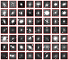 |
Fig. A.1. Cutouts of all dwarf galaxies produced by collapsing the MUSE data cubes along the wavelength axis, resulting in 2D images. The size of the cutouts are chosen to be the diameter of the dwarf’s visual appearance in the MUSE image plus a margin of 2 arcsec. |
A.2. Error estimation
In this section we show the results of the error estimation via MC simulations. The signs of the residuals between the galaxy spectrum and best fit are flipped randomly and refitted with pPXF. This was done in 400 realizations per galaxy which resulted in distributions for the extracted properties velocity, age, and metallicity. In some cases the best-fit value lies outside of the 1σ confidence interval from the MC realizations (see Figure 5). In Figure A.2 we show the residual of the best fit minus the mean and median of the MC realizations, and indicate by color whether or not the best-fit value lies within (green) or outside (red) the 1σ bounds of the MC simulations.
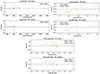 |
Fig. A.2. Residual plots of pPXF best-fit values subtracted by mean and median of the MC realizations for the parameters: recessional velocity (v; top left), age (top right), metallicity (bottom center). The green dots indicate that the best-fit value resides inside the 1σ bounds of the MC realizations; red means the value is outside of these bounds. |
A.3. Data table
We summarize the properties of the 56 dwarfs studied in this work in Table A.1. We obtained the values from Habas et al. (2020), Poulain et al. (2021), and this work.
Properties of the dwarf galaxies studied in this work.
All Tables
All Figures
|
Fig. 1. Examples of different quality spectra with different S/N values. Shown is the relative flux on the y-axis and the wavelength on the x-axis (in angstroms). These spectra have not been shifted to the rest frame. The black line is the galaxy spectrum and the red line the fit produced by pPXF. The gray regions were manually masked out to improve the fit. From top to bottom are shown the spectra for the galaxies MATLAS-269, MATLAS-1232, and MATLAS-10 with S/N values of 8.7, 26.0, and 61.9, respectively. |
| In the text | |
|
Fig. 2. Comparison of dwarf spectra from visually intuited aperture (top) vs. S/N optimized aperture (bottom). Right: stacked MUSE cube of the dwarf MATLAS-445. The spectra were extracted from the colored regions. The S/N was improved from 29.3 (visually intuited aperture) to 32.4 (optimized aperture) for this galaxy. |
| In the text | |
|
Fig. 3. Distributions of signal-to-noise ratios and corresponding optimized apertures from which the spectra were extracted. Top: distribution of S/N values for the sample of dwarf galaxies analyzed in this work. Bottom: distribution of S/N optimized apertures for the dwarf galaxies studied in this work. |
| In the text | |
|
Fig. 4. Comparison of photometric properties with S/N optimized apertures. Top: comparison between S/N optimized radius from this work and the effective radius from Poulain et al. (2021). The black dashed line indicates the equality of the two measurements. Bottom: distribution of the dwarf g-band surface brightness from Poulain et al. (2021) at the radius that optimizes the S/N of the extracted spectrum. |
| In the text | |
|
Fig. 5. Results from the MC error estimation with 400 iterations for the galaxy MATLAS-269. The histograms show the distributions of the fit values for the recessional velocity V, the age, and the metallicity obtained from pPXF by randomly flipping the sign of the residual between the galaxy spectrum and the initial best fit. The solid lines indicate the best-fit values of the original spectrum, while the dashed lines show the standard deviation of the MC realizations. For the recessional velocity shown in the leftmost panel, we fit a Gaussian curve (dashed line) to the distribution of MC realizations. |
| In the text | |
|
Fig. 6. Distribution of measured dwarf line-of-sight velocities studied in this work. The first peak corresponds to the velocity space, which is consistent with the hosts targeted in the ATLAS3D survey. |
| In the text | |
|
Fig. 7. Projected distance between satellite and assumed host galaxy in kpc vs. recessional velocity difference between satellite and host (ΔV = Vsat − Vhost) in km s−1. The projected distance and velocity difference to the host assumed in MATLAS are plotted (gray circles) compared with the updated host based on minimal ΔV through MUSE spectral fitting (red points). These shifts are indicated by black arrows. For the red points circled in gray the assumed host stays the same with new velocity information on the dwarf. The dashed black lines show ±300 km s−1. |
| In the text | |
|
Fig. 8. Photometric properties of MATLAS subsample targeted with MUSE (red) and overall distribution of the MATLAS dwarf galaxies (gray) with robust GALFIT modeling. Top left: Sersic index; top right: apparent g-band magnitude mg; bottom left: effective radius reff; bottom right: axis ratio. |
| In the text | |
|
Fig. 9. Scaling relation absolute g-band magnitude Mg vs. effective radius reff in kpc. Comparison between the dwarf sample studied in this work (red) and the overall MATLAS sample (gray). To get these measurements for the sample with MUSE observations, the associated host galaxy is used to estimate the distance; if not available, the dwarf velocity via Hubble’s law is used. |
| In the text | |
|
Fig. 10. Plot of universal stellar mass-metallicity relation from Kirby et al. (2013; blue solid line) with its rms (blue dashed lines). On the x-axis is plotted the logarithm of the stellar mass in units of solar mass. Left: data from this work (red circles), but excluding star forming and low S/N galaxies. Right: full sample from this work. Star forming galaxies are shown as yellow upward pointing triangles, while low S/N galaxies are gray downward pointing triangles. Shown is a comparison of our results with galaxies from other works: LG dwarfs (blue; Kirby et al. 2013), Cen A dwarfs (pink; Müller et al. 2021b), galaxies in Fornax and Virgo (green; Fahrion et al. 2021), nucleated dwarf LTGs (purple; Fahrion et al. 2022), and UDGs in the Coma cluster (orange; Chilingarian et al. 2019). Bottom: residual plots (i.e., metallicity dwarf-metallicity fit). The blue dashed lines indicate the rms of the fit from Kirby et al. (2013). The LG dwarf metallicities from Kirby et al. (2013) are iron metallicities ([Fe/H]), while all other data points show total metallicities ([M/H]). |
| In the text | |
|
Fig. 11. Mean metallicity as a function of different degrees of spectrum deterioration for the highest S/N dwarf in the sample (MATLAS-553; S/N ∼ 62). The error bars on the y-axis show the standard deviation of 100 MC realizations for every σ. The best-fit value for the metallicity is −1.29 dex. |
| In the text | |
|
Fig. 12. Residuals between metallicities for our dwarfs and the MZR from Kirby et al. (2013) as a function of the local density parameter ρ10. |
| In the text | |
|
Fig. 13. Age vs. metallicity. The dwarf galaxies presented in this work are shown as red circles, yellow upward pointing triangles (star forming), and gray downward pointing triangles (low-quality spectra). Shown is a comparison with the results from other studies: galaxies in the Fornax and Virgo clusters (green; Fahrion et al. 2021), nucleated dwarf LTGs (purple; Fahrion et al. 2022), Cen A dwarfs (pink; Müller et al. 2021b), and UDGs in the Coma cluster (orange; Chilingarian et al. 2019). |
| In the text | |
|
Fig. A.1. Cutouts of all dwarf galaxies produced by collapsing the MUSE data cubes along the wavelength axis, resulting in 2D images. The size of the cutouts are chosen to be the diameter of the dwarf’s visual appearance in the MUSE image plus a margin of 2 arcsec. |
| In the text | |
|
Fig. A.2. Residual plots of pPXF best-fit values subtracted by mean and median of the MC realizations for the parameters: recessional velocity (v; top left), age (top right), metallicity (bottom center). The green dots indicate that the best-fit value resides inside the 1σ bounds of the MC realizations; red means the value is outside of these bounds. |
| In the text | |
Current usage metrics show cumulative count of Article Views (full-text article views including HTML views, PDF and ePub downloads, according to the available data) and Abstracts Views on Vision4Press platform.
Data correspond to usage on the plateform after 2015. The current usage metrics is available 48-96 hours after online publication and is updated daily on week days.
Initial download of the metrics may take a while.