| Issue |
A&A
Volume 699, July 2025
|
|
|---|---|---|
| Article Number | A207 | |
| Number of page(s) | 10 | |
| Section | Extragalactic astronomy | |
| DOI | https://doi.org/10.1051/0004-6361/202452923 | |
| Published online | 07 July 2025 | |
MUSE observations of dwarf galaxies and a stellar stream in the M 83 group⋆
1
Institute of Physics, Laboratory of Astrophysics, Ecole Polytechnique Fédérale de Lausanne (EPFL), 1290 Sauverny, Switzerland
2
Institute of Astronomy, Madingley Rd, Cambridge CB3 0HA, UK
3
Visiting Fellow, Clare Hall, University of Cambridge, Cambridge, UK
4
European Southern Observatory, Karl-Schwarzschild Strasse 2, 85748 Garching, Germany
5
Department of Astrophysics, University of Vienna, Türkenschanzstraße 17, 1180 Wien, Austria
6
European Space Agency, European Space Research and Technology Centre, Keplerlaan 1, 2201 AZ Noordwijk, The Netherlands
7
Leibniz-Institut für Astrophysik Potsdam (AIP), An der Sternwarte 16, D-14482 Potsdam, Germany
8
Observatoire Astronomique de Strasbourg (ObAS), Université de Strasbourg – CNRS, UMR 7550 Strasbourg, France
9
INAF, Arcetri Astrophysical Observatory, Largo E. Fermi 5, 50125 Florence, Italy
10
DARK, Niels Bohr Institute, University of Copenhagen, Blegdamsvej 17, 2100 Copenhagen, Denmark
⋆⋆ Corresponding author: This email address is being protected from spambots. You need JavaScript enabled to view it.
Received:
8
November
2024
Accepted:
21
April
2025
Abstract
Spectroscopy for faint dwarf galaxies outside of our own Local Group is challenging. Here, we present MUSE spectroscopy to study the properties of four known dwarf satellites and one stellar stream (KK 208) surrounding the nearby grand spiral M 83, which resides together with the lenticular galaxy Cen A in the Centaurus group. This data completes the phase-space information for all known dwarf galaxies around M 83 down to a completeness of −10 mag in the V band. All studied objects have an intermediate to old and metal-poor stellar population and follow the stellar luminosity-metallicity relation defined by the Local Group dwarfs. For the stellar stream, we serendipitously identify a previously unknown globular cluster that is old and metal-poor. Two dwarf galaxies (NGC 5264 and dw1341-29) may be a bound satellite of a satellite system due to their proximity and shared velocities. With our access to the positions and velocities of 13 dwarfs around M 83, we estimated the mass of the group with different estimators. Ranging between 1.3 and 3.0 × 10¹² M⊙ for the halo mass, we find it to be larger than previously assumed. This may impact the previously reported tension for cold dark matter cosmology with the count of dwarf galaxies. In contrast to Cen A, we do not find a corotating plane of satellites around M 83.
Key words: galaxies: distances and redshifts / galaxies: dwarf / galaxies: groups: general / galaxies: kinematics and dynamics / dark matter
Based on observations collected at the European Organisation for Astronomical Research in the Southern Hemisphere under ESO program 112.262H.
© The Authors 2025
 Open Access article, published by EDP Sciences, under the terms of the Creative Commons Attribution License (https://creativecommons.org/licenses/by/4.0), which permits unrestricted use, distribution, and reproduction in any medium, provided the original work is properly cited.
This article is published in open access under the Subscribe to Open model. This email address is being protected from spambots. You need JavaScript enabled to view it. to support open access publication.
1. Introduction
The Centaurus group is one of the closest neighbors of our own Local Group. It is made up of two giant galaxies, the lenticular galaxy Cen A at 3.8 Mpc (Harris et al. 2010) and the grand design spiral galaxy M 83 at 4.9 Mpc (Jacobs et al. 2009). Each comes with its own set of dwarf galaxy satellites. Past surveys doubled the number of known dwarf galaxies around Cen A (Crnojević et al. 2014, 2016; Müller et al. 2017a; Taylor et al. 2018) and increased the numbers by 30% around M 83 (Müller et al. 2015), while putting the completeness of known dwarfs on a par with the classical regime of dwarf galaxies within our Local Group (down to MV ≈ −10 mag). The confirmation of dwarf galaxy membership was mainly done by measuring the tip of the red giant branch (Müller et al. 2018a, 2019a; Crnojević et al. 2019), getting distances with an accuracy of 5 to 10%. Other characterizations of properties, such as their velocities or stellar populations, require spectroscopy, which is a much more time-consuming task, especially for the quenched dwarf spheroidals without emission lines. Fortunately, with facilities such as the Very Large Telescope (VLT) getting the necessary spectroscopy to measure these properties is within reach.
The Cen A galaxy group, being closer and more populated than the M 83 group, has been used for extending near-field cosmology tests. Müller et al. (2019a) compared the abundance of the dwarf galaxies around Cen A with expectations from cosmological simulations and found an agreement within 2σ. More puzzling though in the context of Λ cold dark matter (ΛCDM) cosmology is the arrangement and motion of dwarf galaxies around Cen A. The dwarf galaxies are arranged in a thick disk (Tully et al. 2015; Müller et al. 2016), in which the dwarfs are co-moving based on their line-of-sight velocities (Müller et al. 2018b, 2021a), which may indicate corotation (Kanehisa et al. 2023). This is at odds with ΛCDM at the 3σ level. This is reminiscent to the Local Group, where two such corotating planes have been discovered around the Milky Way (Kroupa et al. 2005; Metz et al. 2008; Pawlowski et al. 2012) and the Andromeda galaxy (Koch & Grebel 2006; McConnachie & Irwin 2006; Ibata et al. 2013) and pose a challenge to ΛCDM (see e.g., the reviews by Pawlowski 2021 and Sales et al. 2022).
M 83 is farther away and less populated than Cen A, making such cosmological tests more difficult. Nevertheless, Müller et al. (2024a) compared the abundance of the dwarf galaxies around M 83 with expectations from ΛCDM. In this case, however, the count was too high compared to the expectations at a 3 to 5σ level, depending on how the ΛCDM predictions are made (either through a comparison to cosmological simulations or using the stellar-halo mass relation).
Müller et al. (2018a) suggested the existence of a plane of satellites around M 83 based on the 3D distribution of dwarf galaxies, but noted that the uncertainties are as large as the dimensions of this plane. However, this putative plane is seen edge-on, meaning that if it is indeed a rotationally supported planar structure, we would find a signature with line-of-sight velocity observations, namely that the dwarfs on one side should be redshifted, and on the other side blueshifted, with respect to the group’s mean motion. Such velocity information was only available for eight dwarf galaxies and was inconclusive. Here, we present follow-up observations with the VLT to acquire accurate spectroscopy and derive the line-of-sight velocities of the five remaining known dwarf galaxies (including a tidally disrupting one). Except for dw1341-29, all of them were already confirmed members of the M 83 based on distance measurements through the tip of the red giant branch. The spectroscopy also allows us to estimate the stellar population properties of these targets and search for compact stellar objects such as star clusters.
The manuscript is organized as follows. In Section 2 we present the observations and data reduction, in Section 3 the luminosity-metallicity relation, in Section 4 the discovery of a globular cluster, in Section 5 the phase-space distribution of the dwarf galaxies, and in Section 6 several mass estimations for the M 83 group. Finally, in Section 7 we discuss the results and draw our conclusions.
2. Observations, data reduction, and spectroscopy
The data were collected through the European Southern Observatory (ESO) program 112.262H (PI: Müller) using the Multi Unit Spectroscopic Explorer (MUSE; Bacon et al. 2010, 2012) on UT4 of the VLT at Cerro Paranal, Chile. MUSE is an integral field spectrograph (IFS) with a 1 × 1 arcmin2 field of view, spatial sampling of 0.2 arcsec/pixel, a nominal wavelength range of 480–930 nm, and a resolving power between 1740 (480 nm) and 3450 (930 nm). From a list of confirmed dwarf galaxies around M 83 (Müller et al. 2024a), we observed the remaining five dwarf galaxies without velocity information, listed in Table 1. We note that for one dwarf galaxy, dw1341-29, the value from surface brightness fluctuation measurements is closer to the distance of Cen A, but the large uncertainties makes it plausible that it is a member of M 83 as well. Here, we assume that it is a satellite member of M 83, based on its projected proximity to M 83 and its derived velocity being equal to a nearby dwarf (making it a potential satellite of a satellite, see below).
Observed dwarf galaxies and globular cluster with MUSE.
For one object – the tidally disrupted dwarf KK 208 – we took additional sky exposures because the target filled the MUSE field of view. The total exposure time for this object was 1813s and 453s for the target and sky stacks, respectively. For the remaining objects, we observed on target for a total of 2559s with no extra sky exposures. The MUSE data products, processed through the standard MUSE pipeline (Weilbacher et al. 2012, 2020), are available via the ESO Science Archive. This processing included bias and flat-field corrections, astrometric calibration, sky subtraction, and wavelength and flux calibration (Hanuschik 2020)1.
For sky subtraction, we used the data cube directly where possible for the dwarf galaxies that are small enough to leave sufficient space for sky estimation, eliminating the need for separate sky exposures. Müller et al. (2021b) suggest that with 20% of the MUSE field available for sky subtraction, better results are achieved using the science data cube instead of including a separate sky offset. For KK 208, we still got better results by deriving the sky on a small area within the science exposure rather than the sky exposure. To reduce the sky residual lines, we applied the Zurich atmosphere purge (ZAP) principal component analysis algorithm (Soto et al. 2016). We used the Python implementation (Barbary 2016, SEP) of Source Extractor (Bertin & Arnouts 1996) with a sigma threshold of 0.5 to select empty sky patches, creating a segmented FITS file of all detected sources. Additionally, we added a generous elliptical mask over the dwarf galaxies, because often SEP did not segment their outskirts. This segmentation map was used as a mask for ZAP.
To extract the integrated spectrum of the galaxy body, we used an elliptical aperture adjusted on the collapsed cubes and used SEP to mask foreground stars and background objects, with threshold being between one to ten sigma. Additionally, we manually masked objects as needed. Further, we masked regions that had a median value of 0.1 or lower. This removed empty regions without any signal. The centroid, ellipticity, and position angle of the ellipse were chosen by hand on the white image (i.e., the stacked data cube). The white image and the aperture are shown in Fig. 1.
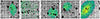 |
Fig. 1. Stacked MUSE cubes. The colored areas indicate the regions where the spectra were extracted. The magenta circle indicates the GC discovered around KK 208. |
To determine the line-of-sight velocities and stellar population properties, we employed the Python implementation of the penalized PiXel-Fitting (pPXF, Cappellari & Emsellem 2004; Cappellari 2017) algorithm, following the procedures used in previous studies with MUSE and pPXF (see Emsellem et al. 2019; Fensch et al. 2019; Müller et al. 2020, 2025; Fahrion et al. 2020a, 2022; Heesters et al. 2023 for more details). We utilized single stellar population (SSP) spectra from the eMILES library (Vazdekis et al. 2016), covering metallicities from solar to –2.27 dex and ages from 70 Myr to 14.0 Gyr, with a Kroupa initial mass function Kroupa 2001. The SSP library spectra were convolved with the line-spread function following Guérou et al. (2017) and detailed in Emsellem et al. (2019). A variance spectrum derived from the masked data cube was incorporated into pPXF to enhance the fitting process. For the kinematic fit, we used 8 degrees of freedom for the additive polynomial and 12 degrees for the multiplicative polynomial (Emsellem et al. 2019). In the age and metallicity fits, we constrained the velocity, omitted additive polynomials, and maintained the 12th degree in the multiplicative polynomial (Fensch et al. 2019). We used pPXF weights to compute mean metallicities, mean ages, and stellar mass-to-light ratios from the SSP models for each galaxy. These stellar population properties are mass-weighted. To improve the fits, we masked residual sky lines not removed by ZAP. The spectra and best-fit models, together with some of the major absorption line regions (Hβ, Mgb, Fe, Hα, and CaT), are presented in Fig. 2, and the derived properties are compiled in Table 1.
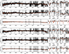 |
Fig. 2. Spectra and zoom-ins around absorption lines of the observed dwarf galaxies. The spectra (black line) and the best fit from pPXF (red line) are plotted in the left panel over the full spectral coverage of MUSE. The gray areas indicate masked regions. The middle and right panels show the two most prominent absorption line regions to derive the velocities, namely the region around Hα and the Calcium Triplet (CaT). |
Uncertainties on the best-fit parameters were estimated using a Monte Carlo method, whereby residuals were reshuffled in a bootstrap approach, with uncertainties given as the 1σ standard deviation of the posterior distribution. The signal-to-noise ratio (S/N) per pixel was calculated in a region between 660 and 680 nm, devoid of strong absorption or emission lines, as the mean fraction between flux and the square root of the variance, multiplied by the χ2 value estimated by pPXF. Since the main objective was to measure line-of-sight velocities, the targeted S/N was 5, and caution is advised regarding age and metallicity estimates. Based on tests of the recovery of SSP input parameters as a function of the S/N with pPXF, Fahrion et al. 2019 suggest that a S/N of > 10 is needed to determine metallicity within 0.2 dex with MUSE, and such ratios are achieved only for one target (KK 218). For ages, an even larger S/N of > 15 is needed for a constraint within 1 Gyr; below, it scatters with almost ±5 Gyr. Again, only KK 218 achieves this S/N (S/N = 22). The other dwarfs have age estimates between 6 to 12 Gyr and can therefore be considered to be of intermediate (2–8 Gyr) to old (> 8 Gyr) age, but we omit the values in Table 1 and only show the ones that have a secured estimate.
To find any compact objects associated with the dwarfs, namely globular clusters or nuclear star clusters, we used the SEP segmentation map of all MUSE stacks as an input of x and y positions. For each segmented object, we used a small circular aperture and extracted the spectrum within, weighting the spectra of each spaxel with a PSF (approximated with a Gaussian) to boost the signal. We visually inspected each spectrum and its derived parameters. For KK 208, we detected a globular cluster, which is also presented in Fig. 2, and in Table 1. No other compact stellar object associated with the dwarfs was found.
To estimate the structural properties of the globular cluster around KK 208, we performed aperture photometry on Legacy Survey data (Dey et al. 2019) in the g and r bands. The effective radius was estimated by modeling the object using a Sérsic profile with Galfit (Peng et al. 2002). We used two different stars in the MUSE field of view as a PSF model. The known dwarf galaxy system surrounding M 83 is listed in Table 2.
Currently known dwarf galaxy system of M 83.
3. The luminosity-metallicity relation
The stellar bodies of dwarf galaxies follow a relation in mass and/or luminosity and metallicity: the fainter – and thus less massive – a galaxy becomes, the more metal-poor it is. This was found first for the dwarf irregular galaxies in the Local Group (Skillman et al. 1989) and later extended to nearby dwarf irregulars (Lee et al. 2006). Lee et al. (2006) showed that the mass-metallicity relation established for large galaxies (Tremonti et al. 2004) extends to the dwarf galaxy regime. Using high-quality data for Local Group dwarf spheroidal galaxies, Kirby et al. (2013) showed that the mass-metallicity relation holds all the way from large galaxies to dwarfs, and also considered metallicities based on absorption line measurements (e.g., Gallazzi et al. 2005).
With modern facilities, it is possible to estimate metallicities for dwarf galaxies outside our own Local Group. Most recently, Heesters et al. (2023) observed 56 dwarf galaxies from the MATLAS survey (Habas et al. 2020; Poulain et al. 2021) with MUSE and found an offset with respect to the Local Group dwarfs’ luminosity-metallicity relation toward more metal-poor stellar populations. Additional observations of nine dwarf galaxies in the MATLAS survey with MUSE strengthened this trend (Müller et al. 2025). However, it is not clear whether this has a physical or systematic cause due to the way the metallicities are measured (fitting CaT absorption lines on individual stars or the multiple lines of the integrated stellar body of the galaxy).
We show the luminosity-metallicity relation of the M 83 dwarfs in Fig. 3 and compare it to the MATLAS dwarfs observed with MUSE, the M 31 dwarfs, and observations of Cen A dwarfs with MUSE (Müller et al. 2021b). We find that the M 83 (and Cen A) dwarfs follow the luminosity-metallicity relation expected from the Local Group dwarfs (Kirby et al. 2013) within ∼3σ (including the uncertainty). However, we note that in the mass range where the dwarf galaxies in the MATLAS survey deviate most from the relation (between 107.0 to 108.5 L⊙), the observed M 83 dwarf’s value is at the lower 3σ limit. However, this is KK 208, which has a low S/N, and therefore large uncertainties. Compared to the MATLAS dwarfs, the Centaurus dwarfs (which include the Cen A dwarfs and the M 83 dwarfs), seem to generally follow the luminosity-metallicity relation. This is striking, because the code used for the MATLAS and Centaurus dwarfs is essentially the same, indicating that the deviation may not come from systematics alone but rather be physical in nature.
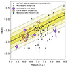 |
Fig. 3. Luminosity-metallicity relation for a reference sample of dwarf galaxies from the MATLAS survey (Heesters et al. 2023; Müller et al. 2025), the ultra-diffuse galaxy NGC 1052-DF2 (Fensch et al. 2019), the Cen A dwarfs (Müller et al. 2021b), and the M 83 dwarf galaxies observed here. The line and intervals indicate the fit by Kirby et al. (2013) for the Local Group dwarfs and the 1, 2, and 3σ intervals. |
4. The globular cluster of KK 208
The velocity of the stellar body of KK 208 is 439.9 ± 15.6 km/s and that of the globular cluster found in the MUSE pointing is 432.08 ± 3.3 km/s. These values are consistent with each other. The globular cluster is therefore likely associated with the dwarf galaxy. It seems unlikely that the globular cluster could be a contaminant star, according to the Besançon model of Galactic foreground stars (Robin et al. 2003). The expected velocity distribution for the Milky Way stars in the direction of M 83 is well approximated by the sum of two Gaussian profiles, with means of VBes, 1 = −3 km/s, VBes, 2 = 76 km/s, and standard deviations of σBes, 1 = 38 km/s, σBes, 2 = 102 km/s. Therefore, the objects velocity is at the tail end of the velocity distribution, more than 3 sigma above the mean. The line-of-sight velocity of M 83 is vM83 = 519 ± 18 km/s, which is further away from the velocity of the globular cluster. While it is still reasonable to assume that it could be a GC in the halo of M 83, the closeness in phase-space to KK 208 makes this unlikely and we conclude that it is a GC associated with KK 208.
In Fig. 4, we show the white image of the GC and the Sérsic subtracted residual image. We note that there is a residual in the center, which is typical for slightly extended objects. In Fig. 4, we also show the normalized radial profile of the GC, as well as a radial profile of two PSF stars. It is evident that the globular cluster is marginally resolved, with more extended wings compared to the PSF. This is expected. GCs at the distance of Cen A/M 83 are partly resolved, showing broader and less peaked light distributions when compared to the stellar PSF (see e.g. Fig 1 in Rejkuba 2001).
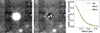 |
Fig. 4. Globular cluster associated with KK 208. Left: MUSE stacked image. Middle: Sérsic model subtracted image. Right: Normalized radial profile of the globular cluster (black line) associated with KK 208 and two PSF stars (dashed orange lines). The vertical gray line indicates the half-light radius of the globular cluster estimated by Galfit. |
We measured the size of the GC using
 (1)
(1)
and
 (2)
(2)
where FWHMGC = 0.40 arcsec and FWHMPSF = 0.33 arcsec correspond to the measured full width half max of the GC and PSF, respectively. At the distance of KK 208, this translates into 5.6 pc. Calculating σGC from this, we estimate an effective radius of 2.4 pc for the GC. At a distance of 5.01 Mpc for KK 208 (Anand et al. 2021) and correcting for galactic extinction, we find an absolute magnitude of −5.5 mag in the V band for the globular cluster. The size and brightness of the GC are typical for such objects (e.g., Georgiev et al. 2009).
With a metallicity estimate of [M/H]= − 1.48 ± 0.04 dex and an age estimate of 13.7 ± 1.6 Gyr, the globular cluster of KK 208 is consistent with measurements of other globular clusters observed with MUSE (see Fig. 5) and has a stellar mass of 3.0 × 10⁴ M⊙. It is old and metal-poor and has a similar metallicity as its host KK 208 ([M/H]= − 1.53 ± 0.23 dex).
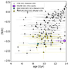 |
Fig. 5. Age-metallicity relation for a reference sample of globular clusters from the F3D survey (Fahrion et al. 2020b), the ultra-diffuse galaxy MATLAS-2019 (Müller et al. 2020), the stacked clusters of the ultra-diffuse galaxy NGC 1052-DF2 (Fensch et al. 2019), and the globular cluster of KK 208 observed here. |
5. The phase-space distribution of the satellites
Now that we have a complete set of dwarf galaxies around M 83 with both confirmed membership from distances and velocities, we can study the phase-space distribution of the satellite system.
5.1. The dwarf galaxy population
Müller et al. (2018a) studied the spatial distribution of the satellites around M 83 and noted that a 3D analysis is unfeasible compared to the studies in the Local Group and Cen A. This is due to the fact that the average distance uncertainties are on the order of ≈300 kpc, which is larger than the virial radius of the host. Therefore, we have solely worked with projected distances. First, we estimated the geometry. For that, we applied a principle component analysis, which returns the eigenvectors corresponding to the major and minor axes of the projected satellite distribution. These vectors are indicated in Fig. 6. The minor-to-major axis ratio is 0.65, with a semimajor axis length of 111 kpc. As is seen in Fig. 6, there are two dwarf galaxies outside of the virial radius (see Sect. 6 for the calculation of the radius): KK195 and HIDEEPJ1337-33. While the former is within the extension of the major axis, the latter is almost perpendicular to it and rather isolated. Removing the two, and repeating the analysis (effectively studying the dwarfs within the virial radius), we get a semimajor axis of 92 kpc and a ratio of 0.44. In both cases, the flattening is not strong.
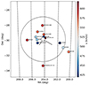 |
Fig. 6. Field around M 83 (large white dot) and its surrounding dwarfs (colored dots) in equatorial coordinates (J2000.0). The colors represent the line-of-sight velocity of the galaxies, as is indicated with the color bar. The two black lines correspond to the minor and major axes of the satellite system (see text), and the circle to the virial radius. |
We next investigated the motion of the satellites within the system. For that, we projected their distances from the minor axis (derived from the full sample) along the major axis, centered on M 83. As a convention, we assigned negative distances to the left side of the minor axis (i.e., in the direction of a larger RA). In Fig. 7, we plot the line of sight velocity as a function of the projected distance and split the figure in four quadrants. A fully rotationally supported system will occupy two opposing quadrants, whereas a fully pressure-supported and isotropically distributed system will occupy all four equally. For M 83, we find no signal for a rotationally supported system, with 7/13 and 6/13 satellites being on opposing quadrants, respectively. To summarize, we find neither a significant flattening nor signals of corotation for the M 83 satellite system aligned with this flattening.
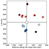 |
Fig. 7. Position velocity diagram of the satellite system (small colored dots) of M 83 (large white dot). The x axis corresponds to the projected distance along the major axis of the satellite system, and the y axis to the line-of-sight velocities. The color coding corresponds to the velocity and is the same as for Fig. 6. |
The dwarf galaxy dw1335-29 has a higher velocity than the rest of the system. This is evident in Fig. 7. The 1σ standard deviation of the velocity of the full satellite system is 81 km/s. With a relative velocity to M 83 of 187 km/s, dw1335-29 is at the 2.3σ tail of the distribution. It is the closest system to M 83, with a projected separation of only 27 kpc, and may therefore be on or close to its pericenter. Notably, the tidally disrupted dwarf KK 208 is close by in projection to dw1335-29 (see Fig. 10 in Müller et al. 2018a); however, the two have a velocity difference of 266 km/s, making an association unlikely.
5.2. A satellite-of-a-satellite system
Two dwarf galaxies are close in phase-space. They are NGC5264 and dw1341-29. Their projected separation is only 32 kpc and they share a common velocity, 478 ± 9 km/s and 483 ± 20 km/s, respectively. NGC 5264 has an absolute V band magnitude of −16.7 (4.1 × 10⁸ L⊙) and is the brightest satellite of M 83, while dw1341-29 is the faintest satellite discovered so far, with −8.8 mag (2.8 × 10⁵ L⊙). They have a luminosity ratio of 1445. This pair may be a satellite-of-a-satellite system. We quantify this below.
Geha et al. (2010) provided a criterion for a pair of satellites to be bound when
 (3)
(3)
where Δr is the physical separation between the objects, Δv is their total velocity difference, Mpair is the total mass of the pair, and G is the gravitational constant. Using this formula, we can solve for the minimal mass, Mpair, to be bound by assuming b ≈ 1. We find that Mpair > 9.3 × 10⁷ M⊙ to be considered bound. Including the uncertainties in distance (taking half the projected distance as uncertainty in depth) and velocity, we find a conservative criteria of Mpair > 2.6 × 10⁹ M⊙. For the former, the stellar mass of NGC 5264 (8 × 10⁸ M⊙, using a stellar M/L ratio of two to transform the luminosity into a stellar mass) alone is large enough to satisfy this criteria. For the latter, the pair would need only three times the observed stellar mass in form of gas or dark matter to satisfy the criteria. This is realistic (see e.g., Fig. 11 in McConnachie 2012), with dwarf galaxies at this luminosity hosting such dark matter halos. We therefore conclude that dw1341-29 is a bound satellite of NGC5264 and that the two represent a satellite-of-a-satellite system.
6. Mass estimations of the M 83 group
In the following, we compare different methods of deriving the mass of the M 83 halo. Since we did not detect any sign of coherent rotation of the satellite system, we did not include any correction for possible rotation when using the satellites as tracers.
6.1. Virial theorem
Previously, the mass was estimated by Karachentsev et al. (2002, 2007) based on the virial theorem. We used their equation,
 (4)
(4)
where N is the number of tracers, G the gravitational constant, σlos the measured velocity dispersion along the line of sight, and ⟨Rij⟩ the mean pairwise projected separation between the dwarf galaxies. For the M 83 group, we find higher values for both σlos and ⟨Rij⟩ compared to Karachentsev et al. (2007). We estimate σlos = 80.6 ± 15.4 km/s and RH = 163 kpc (compared to 61 km/s and 89 kpc, respectively). This leads to a higher mass estimation for M 83, namely Mvir = 2.5 ± 0.7 × 10¹² M⊙ (compared to 0.8 × 10¹² M⊙, Karachentsev et al. 2007). The errors were estimated by Monte Carlo simulations. First, a new set of velocities was created for each iteration by drawing the velocity from a Gaussian distribution with the mean set as the observed velocity and the standard deviation corresponding to the velocity uncertainties. These new velocities were randomly assigned to the dwarfs. Then, we sampled from the dwarf galaxy catalog by drawing between 8 and 13 dwarfs for each iteration. The 1σ bound in log space of the Mvir posterior gives the uncertainties.
6.2. Density contrast
We examined whether the updated virial mass of M 83 is realistic. In a ΛCDM cosmological context, the masses of galaxy groups can be estimated for a density contrast, Δ, with respect to the critical density of the Universe, ρc. The radius, RΔ, defines the volume where the density is equal to Δρc. If we assume that the measured flat part of the rotation curve of M 83 – vflat = 190 km/s (Dykes et al. 2021) – corresponds to the circular velocity, vcirc, at the radius, RΔ, the total encompassed mass (baryons and dark matter) is given by (see, e.g. McGaugh 2012)
 (5)
(5)
where H0 = 75.1 ± 3.8 km/s/Mpc (Schombert et al. 2020) is the Hubble constant2, and RΔ is given by
 (6)
(6)
Adopting the commonly used value of Δ = 200, we derived for the M 83 group a mass of M200 = 2.1 ± 0.3 × 10¹² M⊙ within R200 = 253 ± 0.3 kpc. The uncertainties were derived by assuming an uncertainty of 10 km/s for the rotation curve measurement. This mass estimate is consistent with the mass estimate following the virial theorem we derived before (Mvir = 2.5 ± 0.7 × 10¹² M⊙) and is higher than the values suggested by Karachentsev et al. (2007).
6.3. Abundance matching
Using abundance matching, we can directly estimate the halo mass from the stellar mass of M 83. Using Table 3 of Behroozi et al. (2010) as a look-up table (and interpolating between their data points), we derived a halo mass for M 83 of MAM = 3.0 ± 0.5 × 10¹² M⊙. The error was derived by assuming a 10 percent uncertainty on the stellar mass of M 83. This value is higher than the previous two estimates, but still within 1 to 2σ, and thus compatible.
Using the abundance matching relation between the effective radius and R200 (Kravtsov 2013) with an effective radius of M 83 of 3.5 kpc (Leroy et al. 2021), we derived a virial radius of 233 kpc, which is similar to the value estimated from the density contrast (253 kpc). Now, if we estimate the halo mass from the virial radius through the relation
 (7)
(7)
we can get another estimate for the mass through abundance matching. With H0 and Δ as before, we find that MAM, reff = 1.7 ± 0.5 × 10¹² M⊙. This is lower than the Behroozi et al. (2010) abundance matching halo mass by a factor of two. For the estimation of the uncertainties, we used the error on the Hubble constant (3.8 km/s/Mpc, Schombert et al. 2020) and a 10 percent uncertainty on the effective radius.
6.4. Integrated Jeans-based analysis
Another approach to measuring the mass of the M 83 group is through direct Jeans analysis. This has the advantage that we have control over the mass profile and the velocity anisotropy and can factor in these unknown parameters in the error estimation. For a low number of discrete data points, it is, however, advisable to instead use an integrated version of the Jeans equations that avoids binning the already sparse data. Watkins et al. (2010) presented mass estimators to compute the enclosed mass of galaxy halos from samples of discrete positional and kinematical data of tracers, such as dwarf satellites. Among these estimators, there is one for using only projected positions and line-of-sight velocities. An & Evans (2011) expanded on this work. Following their section 4.2, the enclosed mass is given as
 (8)
(8)
where ω(R) is a weighting function and vi is the line-of-sight velocity of the ith tracer. The weighting function was calculated as
 (9)
(9)
and
 (10)
(10)
where Γ(x) is the gamma function, α the power index of the scale-free potential (with α = 1 representing a point mass and α = 0 a logarithmic – i.e., truncated – singular isothermal sphere), and β the anisotropy parameter for the spherical system. In an isothermal system where the radial and tangential dispersions are equal, β = 0. For systems in which the orbits are predominantly radial the anisotropy parameter is β > 0 and for predominantly tangential orbits it is β < 0. Here, we know the values for neither α nor β. Assuming α = 0 and the β = 0.3 based on simulated halos (Mamon et al. 2013), we derive a mass of Mout = 1.5 ± 0.1 × 10¹² M⊙ within rout = 325 kpc (the largest projected separation of a dwarf galaxy to M 83). The uncertainties are based on sampling the velocities of the tracers using their uncertainties around the value as a normal distribution. This, however, does not include varying α or β values. If we allow α to vary between −1.5 and 0.5, and β within a Gaussian distribution centered on log(−β + 1) with β = 0.3 with a standard deviation of 0.3 dex, we can construct a distribution of possible masses. Its standard deviation informs us about the uncertainty. We estimate Mout, possible = 2.2 ± 0.5 × 10¹² M⊙, with the nominal value giving the mean of the distribution. If we calculate the mean density within a sphere with rout = 325 kpc, it is below the critical density we previously calculated using the density contrast by a factor of three. This means that the virial mass must be lower than the value we estimated here; in other words, the estimations are upper limits.
The value estimated through a Jeans-based analysis is still higher than previous literature values, but smaller than the three other approaches we have used in the previous two subsections. Within the uncertainties, all of the values are mutually consistent, though.
6.5. Modified Newtonian dynamics (MOND)
In the context of alternative gravity scenarios, such as MOND (Milgrom 1983), the missing mass is explained by a modification of the laws of gravity rather than by a dark matter particle (e.g., Famaey & McGaugh 2012, and references therein).. In MOND, Newton’s law of gravity is changed for accelerations below the threshold a0 ≈ 10−13 km/s2. In a MOND Universe, one could ask what the dark matter inferred from observations would be when applying Newton’s law of gravity (without any MOND effect). In a MOND cosmology, this would be called phantom dark matter. Oria et al. (2021) explored the predictions of the phantom dark matter mass inferred from the baryonic content of a galaxy in such a scenario. Their Eq. 10 gives a form to calculate the phantom dark matter mass encompassed within a radius, r:
 (11)
(11)
Following the steps in Müller et al. (2019b) to estimate the baryonic mass of spiral galaxies from the K band magnitude, we estimate that Mb = 0.6 × 10¹¹ M⊙ for M 83. This yields a phantom dark matter mass at R200 of MPDM = 1.9 ± 0.3 × 10¹² M⊙, with the uncertainties estimated from a Monte Carlo run where the baryonic mass is assigned an uncertainty of 30 percent and R200 are sampled. This value is consistent with the derived masses for the M 83 halo in the previous four subsections.
7. Discussion and conclusions
With the new MUSE observations of five dwarf galaxies in the vicinity of M 83, we have completed the line-of-sight velocity information for all 13 known dwarfs around M 83. Together with tip of the red giant branch distances for all but one dwarf (dw1341-29, which only has surface brightness fluctuation distances), this yields a complete picture of the M 83 group. Spectroscopic analysis of the five dwarf galaxies reveals that their stellar populations follow the universal luminosity-metallicity relation. The brightest dwarf galaxy (in terms of integrated luminosity) – the tidally disrupted dwarf KK 208 – lies at the 3σ border of the relation, but we note that the S/N is low for accurate spectroscopy. It is still noteworthy that Heesters et al. (2023) found a systematic offset from the relation, on which KK 208 would fall. Better spectroscopy of KK 208 is needed to test this, though.
For KK 208, we discovered a globular cluster in the field of view of MUSE. Based on its velocity, it is associated with KK 208. Its high S/N allowed us to derive accurate age and metallicity properties. It is old and metal-poor, as is expected from observations of other globular clusters around metal-poor dwarf galaxies.
Satellite-of-a-satellite systems have been studied in Müller et al. (2023) with respect to cosmological expectations. There, it was found that observed satellites of satellites are unusually bright (i.e., there is a low luminosity ratio between the dwarf galaxy and its brightest satellite) when compared to state-of-the-art ΛCDM simulations (Revaz & Jablonka 2018), especially in the brightness ranges between 106 to 108 L⊙. The potential satellite pair discovered here – NGC 5264 and dw1341-29 – is at the bright end of their inspected sample, and is likely gravitationally bound based on their common velocity and small separation. The observed pair resembles the model dwarf h021 and its satellite (from Revaz & Jablonka 2018), where the main satellite has a luminosity of 2.3 × 10⁸ L⊙ and the luminosity ratio with its brightest satellite is 865. To compare, NGC 5264 has a luminosity of 4.1 × 10⁸ L⊙ and is 1445 times brighter than dw1341-29. These observed properties are well within the spread of the simulated models. We therefore find that this satellite-of-satellite pair is in agreement with ΛCDM expectations based on the simulations of Revaz & Jablonka (2018). More confirmed satellite of satellite systems need to be studied to test whether they follow the expectations from standard cosmology or not.
The M 83 group forms, together with the Cen A group, the Centaurus aggregation (or Centaurus group). Cen A with its satellite system is one of the best-studied systems outside of our Local Group and was found to host a corotating plane-of-satellites. Compared to high-resolution ΛCDM simulations, such corotating systems are outliers and should be rare. It is therefore natural to ask whether the M 83 group hosts a similar structure. For M 83, it was put forward that there might be a flattened structure based on the 3D distribution of its satellites (see Fig. 9 in Müller et al. 2018a), but at the same time the 3D distance uncertainties are as large as such a putative structure. Also, no kinematic study was conducted. Here, we are using the on-sky projection and motion of the 13 dwarf galaxies around M 83 to study whether there might be a corotating plane of satellites around M 83. We do not find convincing evidence for that, though. Rather, the motion is uncorrelated and, while there is some flattening of the system, it is well consistent with expectations from cosmological simulations. For example, Müller et al. (2024b) find for analogs of the M 81 group in the TNG50 simulation a typical flattening between 0.4 and 0.8 for its 19 satellites with velocity and distance information. The direct comparison to M 81 is valid because their stellar luminosity is similar (log K = 10.95 for M 81 and log K = 10.86 for M 83, according to the updated Local Volume catalog, Karachentsev et al. 2004) and the halo mass range for the selection in TNG50 was set to be between 0.5 and 2.0 ×10¹² M⊙, which is the range of masses we find here for the M 83 halo. With a measured flattening of 0.6 for the M 83 satellite system, it is within 1σ of expectations (see Fig. 6 in Müller et al. 2024b). We conclude that current observations do not support a scenario in which M 83 hosts a corotating plane of satellites seen edge-on and that the system is well within ΛCDM expectations. The Cen A/M83 pair of galaxies is therefore different from the Milky Way and Andromeda galaxy pair when it comes to phase-space correlations.
There are some caveats to consider concerning the non-detection of a coherently moving plane of satellites. We will only be able to detect a corotating plane if it is (a) well-populated and (b) observed under a low inclination. For example, only half the satellites of the Andromeda galaxy make up the corotating plane of satellites. The velocities of the dwarfs outside the plane are uncorrelated in phase-space. If we were to include all dwarf galaxies of the Andromeda galaxy in an analysis such as the one we performed, we would draw similar conclusions as for M 83 (i.e., find no corotating structure). Only by studying the subpopulation of the Andromeda satellite system does the phase-space correlation become significant. The reason why we do not consider subpopulations around M 83, then, is due to sample size. While around the Andromeda galaxy there are more than 20 dwarf galaxies, here we have a sample of 13 dwarfs. The binomial chance of finding a correlated signal with half the population (six dwarfs) would be 3 percent and would not allow us to draw any conclusions at a 3σ level. So, while the subpopulation of dwarfs around the Andromeda galaxy is large enough (15 dwarf galaxies are in the plane) to establish a phase-space correlation, the same is currently not given for M 83. The other caveat is the inclination. Only when seeing a corotating plane of satellites almost edge-on, such as is the case for the Andromeda galaxy or Cen A, are we able to detect them in the first place. A face-on plane or one with a high inclination will be difficult, albeit not impossible to detect. There are ongoing efforts to enable us to detect face-on planes of satellites from line-of-sight velocity measurements and it should in principle be possible to distinguish a corotating plane-of-satellites seen edge-on from a pressure-supported system by the absolute value of the velocity dispersion (Crosby et al., in prep.).
It is interesting to note that the planes of satellites around Cen A and the Andromeda galaxy are aligned with the large-scale structure nearby (Libeskind et al. 2019). In their work, the putative plane of M 83 stands out as an outlier and no alignment with the shear tensors that define the directions of collapse was found. This is now unsurprising, as the existence of the putative M 83 plane is not supported anymore by current data. Other outliers in their analysis were the Milky Way plane, for which we have excellent data supporting the existence of a plane (Pawlowski 2018), and M 101 (Müller et al. 2017b), which was further studied by Anand et al. (2018) and appears to be a filament stretching out from the Local Sheet (see their Fig. 7) and extending several megaparsecs toward NGC 6946 and beyond. It is therefore wrong to conclude that an outlier from the alignment with the shear tensors necessitates that the structure is not real.
With the velocities at hand for the whole satellite system, we can estimate the mass of the M 83 group. Applying the virial theorem, we estimate that the M 83 group has a total mass of 2.5 ± 0.7 × 10¹² M⊙. This mass is consistent with the expected mass derived from the flat part of the rotation curve of M 83 (2.1 ± 0.3 × 10¹² M⊙) and from abundance matching (3.0 ± 0.5 × 10¹² M⊙). The face value is larger than previous estimates but follows from a larger measured velocity dispersion. Using instead an estimator based on Jeans modeling and reasonable assumptions for the velocity anisotropy (β = 0.3) and an isothermal mass profile, we estimate a mass of 1.5 ± 0.1 × 10¹² M⊙. However, when sampling α and β with realistic values, the masses are larger with 2.2 ± 0.5 × 10¹² M⊙. At a 2σ level, all these measurements of the halo mass of M 83 are in line with measurements from our own Milky Way group, ranging between 1.0 to 1.5 × 10¹² M⊙ (Piffl et al. 2014; Posti & Helmi 2019; Shen et al. 2022; Kravtsov & Winney 2024). The halo mass values for M 83 estimated here are larger than previously assumed, which would have an impact on a recent study of the number of expected satellites around M 83 (see next paragraph). The average halo mass from different tracers estimated here is 2.1 ± 1.0 × 10¹² M⊙. This yields a dynamical mass-to-light ratio for the M 83 group of 30, which indicates a dark-matter-dominated halo. As a test for alternative gravity models, namely MOND, we calculated the expected phantom dark matter mass in such a scenario. With a phantom dark matter mass of 1.9 ± 0.3 × 10¹² M⊙, MOND correctly predicts the inferred total mass of M 83 within the uncertainties.
In Müller et al. (2024a), the authors estimated that the count of 13 dwarf galaxies is too large in ΛCDM based on comparisons to cosmological simulations and predictions from the subhalo mass function. Similar findings have been reported for a statistical sample from the MATLAS survey (Kanehisa et al. 2024) and our own Milky Way system (Homma et al. 2024). For the comparison to cosmological simulations, Müller et al. (2024a) used only the baryonic mass of M 83 to select the halos within TNG50 of the Illustris suite (not the halo mass); therefore, the updated total halo mass will not affect their results and the tension remains. For the theoretical predictions from the subhalo mass function, they however assumed halo masses for M 83 between 0.8 to 1.0 × 10¹² M⊙ and found a 5σ to 3σ discrepancy, respectively, with theoretical predictions. The larger the halo mass, the higher the number of expected satellites. A halo mass more than two times as large as the one used in Müller et al. (2024a) will move the tension below the 3σ limit.
It is critical to get an accurate halo mass estimation of M 83 for such kinds of studies. Recently, Hughes et al. (2023), and Dumont et al. (2024) used different tracers such as dwarf galaxies, streams, and globular clusters to update the virial mass of the Cen A group from previous estimations using only the dwarf galaxies (Karachentsev et al. 2002, 2007; Müller et al. 2022). Such an analysis can be extended to the M 83 group. The stream KK 208, especially, may constrain the halo mass of M 83, as was done for Cen A (Pearson et al. 2022). Such an effort might push down the uncertainties and yield more accurate estimations of the halo mass of M 83, which in turn will help constrain cosmological models. Furthermore, wide-area searches for globular clusters and a spectroscopic radial velocity follow-up survey can provide additional constraints for a detailed cosmological mass modeling of M 83.
The value of the Hubble constant is still debated, but ranges between 67 and 75 (Freedman et al. 2019; Planck Collaboration VI 2020; Kourkchi et al. 2020; Khetan et al. 2021; Riess et al. 2021; Javanmardi et al. 2021). We adopted a Hubble constant derived from the baryonic Tully-Fisher relation, which favors higher values.
Acknowledgments
We thank the referee for the constructive report, which helped to clarify and improve the manuscript. O.M. and N.H. are grateful to the Swiss National Science Foundation for financial support under the grant number PZ00P2_202104. M.S.P. acknowledges funding of a Leibniz-Junior Research Group (project number J94/2020). This project has received funding from the European Union’s Horizon Europe research and innovation programme under the Marie Skłodowska-Curie grant agreement No 101103830. SP was supported by a research grant (VIL53081) from VILLUM FONDEN.
References
- An, J. H., & Evans, N. W. 2011, MNRAS, 413, 1744 [Google Scholar]
- Anand, G. S., Rizzi, L., & Tully, R. B. 2018, AJ, 156, 105 [NASA ADS] [CrossRef] [Google Scholar]
- Anand, G. S., Rizzi, L., Tully, R. B., et al. 2021, AJ, 162, 80 [CrossRef] [Google Scholar]
- Bacon, R., Accardo, M., Adjali, L., et al. 2010, in Proc. SPIE, 7735, 773508 [Google Scholar]
- Bacon, R., Accardo, M., Adjali, L., et al. 2012, The Messenger, 147, 4 [NASA ADS] [Google Scholar]
- Banks, G. D., Disney, M. J., Knezek, P. M., et al. 1999, ApJ, 524, 612 [NASA ADS] [CrossRef] [Google Scholar]
- Barbary, K. 2016, J. Open Source Software, 1, 58 [NASA ADS] [CrossRef] [Google Scholar]
- Begum, A., Chengalur, J. N., Karachentsev, I. D., Sharina, M. E., & Kaisin, S. S. 2008, MNRAS, 386, 1667 [NASA ADS] [CrossRef] [Google Scholar]
- Behroozi, P. S., Conroy, C., & Wechsler, R. H. 2010, ApJ, 717, 379 [Google Scholar]
- Bertin, E., & Arnouts, S. 1996, A&AS, 117, 393 [NASA ADS] [CrossRef] [EDP Sciences] [Google Scholar]
- Cappellari, M. 2017, MNRAS, 466, 798 [Google Scholar]
- Cappellari, M., & Emsellem, E. 2004, PASP, 116, 138 [Google Scholar]
- Crnojević, D., Sand, D. J., Caldwell, N., et al. 2014, ApJ, 795, L35 [CrossRef] [Google Scholar]
- Crnojević, D., Sand, D. J., Spekkens, K., et al. 2016, ApJ, 823, 19 [Google Scholar]
- Crnojević, D., Sand, D. J., Bennet, P., et al. 2019, ApJ, 872, 80 [Google Scholar]
- Dey, A., Schlegel, D. J., Lang, D., et al. 2019, AJ, 157, 168 [Google Scholar]
- Dumont, A., Seth, A. C., Strader, J., et al. 2024, A&A, 685, A132 [NASA ADS] [CrossRef] [EDP Sciences] [Google Scholar]
- Dykes, T., Gheller, C., Koribalski, B. S., Dolag, K., & Krokos, M. 2021, Astron. Comput., 34, 100448 [NASA ADS] [CrossRef] [Google Scholar]
- Emsellem, E., van der Burg, R. F. J., Fensch, J., et al. 2019, A&A, 625, A76 [NASA ADS] [CrossRef] [EDP Sciences] [Google Scholar]
- Fahrion, K., Lyubenova, M., van de Ven, G., et al. 2019, A&A, 628, A92 [NASA ADS] [CrossRef] [EDP Sciences] [Google Scholar]
- Fahrion, K., Müller, O., Rejkuba, M., et al. 2020a, A&A, 634, A53 [NASA ADS] [CrossRef] [EDP Sciences] [Google Scholar]
- Fahrion, K., Lyubenova, M., Hilker, M., et al. 2020b, A&A, 637, A26 [NASA ADS] [CrossRef] [EDP Sciences] [Google Scholar]
- Fahrion, K., Bulichi, T.-E., Hilker, M., et al. 2022, A&A, 667, A101 [NASA ADS] [CrossRef] [EDP Sciences] [Google Scholar]
- Famaey, B., & McGaugh, S. S. 2012, Liv. Rev. Relativity, 15, 10 [NASA ADS] [CrossRef] [Google Scholar]
- Fensch, J., van der Burg, R. F. J., Jeřábková, T., et al. 2019, A&A, 625, A77 [NASA ADS] [CrossRef] [EDP Sciences] [Google Scholar]
- Freedman, W. L., Madore, B. F., Hatt, D., et al. 2019, ApJ, 882, 34 [Google Scholar]
- Gallazzi, A., Charlot, S., Brinchmann, J., White, S. D. M., & Tremonti, C. A. 2005, MNRAS, 362, 41 [Google Scholar]
- Geha, M., van der Marel, R. P., Guhathakurta, P., et al. 2010, ApJ, 711, 361 [NASA ADS] [CrossRef] [Google Scholar]
- Georgiev, I. Y., Puzia, T. H., Hilker, M., & Goudfrooij, P. 2009, MNRAS, 392, 879 [NASA ADS] [CrossRef] [Google Scholar]
- Grossi, M., Disney, M. J., Pritzl, B. J., et al. 2007, MNRAS, 374, 107 [NASA ADS] [CrossRef] [Google Scholar]
- Guérou, A., Krajnović, D., Epinat, B., et al. 2017, A&A, 608, A5 [Google Scholar]
- Habas, R., Marleau, F. R., Duc, P.-A., et al. 2020, MNRAS, 491, 1901 [NASA ADS] [Google Scholar]
- Hanuschik, R., & Data Processing,& Quality Control Group, in ESO Calibration Workshop: The Second Generation VLT Instruments and Friends, 15 [Google Scholar]
- Harris, G. L. H., Rejkuba, M., & Harris, W. E. 2010, PASA, 27, 457 [NASA ADS] [CrossRef] [Google Scholar]
- Heesters, N., Müller, O., Marleau, F. R., et al. 2023, A&A, 676, A33 [NASA ADS] [CrossRef] [EDP Sciences] [Google Scholar]
- Homma, D., Chiba, M., Komiyama, Y., et al. 2024, PASJ, 76, 733 [NASA ADS] [CrossRef] [Google Scholar]
- Hughes, A. K., Sand, D. J., Seth, A., et al. 2023, ApJ, 947, 34 [NASA ADS] [CrossRef] [Google Scholar]
- Ibata, R. A., Lewis, G. F., Conn, A. R., et al. 2013, NAT, 493, 62 [NASA ADS] [CrossRef] [Google Scholar]
- Jacobs, B. A., Rizzi, L., Tully, R. B., et al. 2009, AJ, 138, 332 [NASA ADS] [CrossRef] [Google Scholar]
- Javanmardi, B., Mérand, A., Kervella, P., et al. 2021, ApJ, 911, 12 [Google Scholar]
- Kanehisa, K. J., Pawlowski, M. S., Müller, O., & Sohn, S. T. 2023, MNRAS, 519, 6184 [NASA ADS] [CrossRef] [Google Scholar]
- Kanehisa, K. J., Pawlowski, M. S., Heesters, N., & Müller, O. 2024, A&A, 686, A280 [NASA ADS] [CrossRef] [EDP Sciences] [Google Scholar]
- Karachentsev, I. D., Sharina, M. E., Dolphin, A. E., et al. 2002, A&A, 385, 21 [CrossRef] [EDP Sciences] [Google Scholar]
- Karachentsev, I. D., Karachentseva, V. E., Huchtmeier, W. K., & Makarov, D. I. 2004, AJ, 127, 2031 [Google Scholar]
- Karachentsev, I. D., Tully, R. B., Dolphin, A., et al. 2007, AJ, 133, 504 [NASA ADS] [CrossRef] [Google Scholar]
- Karachentsev, I. D., Makarov, D. I., Karachentseva, V. E., & Melnik, O. V. 2008, Astron. Lett., 34, 832 [NASA ADS] [CrossRef] [Google Scholar]
- Karachentsev, I. D., Makarov, D. I., & Kaisina, E. I. 2013, AJ, 145, 101 [Google Scholar]
- Khetan, N., Izzo, L., Branchesi, M., et al. 2021, A&A, 647, A72 [NASA ADS] [CrossRef] [EDP Sciences] [Google Scholar]
- Kirby, E. N., Cohen, J. G., Guhathakurta, P., et al. 2013, ApJ, 779, 102 [Google Scholar]
- Koch, A., & Grebel, E. K. 2006, AJ, 131, 1405 [NASA ADS] [CrossRef] [Google Scholar]
- Koribalski, B. S., Staveley-Smith, L., Kilborn, V. A., et al. 2004, AJ, 128, 16 [Google Scholar]
- Kourkchi, E., Tully, R. B., Eftekharzadeh, S., et al. 2020, ApJ, 902, 145 [NASA ADS] [CrossRef] [Google Scholar]
- Kravtsov, A. V. 2013, ApJ, 764, L31 [NASA ADS] [CrossRef] [Google Scholar]
- Kravtsov, A., & Winney, S. 2024, Open J. Astrophys., 7, 50 [Google Scholar]
- Kroupa, P. 2001, MNRAS, 322, 231 [NASA ADS] [CrossRef] [Google Scholar]
- Kroupa, P., Theis, C., & Boily, C. M. 2005, A&A, 431, 517 [NASA ADS] [CrossRef] [EDP Sciences] [Google Scholar]
- Lee, H., Skillman, E. D., Cannon, J. M., et al. 2006, ApJ, 647, 970 [NASA ADS] [CrossRef] [Google Scholar]
- Leroy, A. K., Hughes, A., Liu, D., et al. 2021, ApJS, 255, 19 [NASA ADS] [CrossRef] [Google Scholar]
- Libeskind, N. I., Carlesi, E., Müller, O., et al. 2019, MNRAS, 490, 3786 [NASA ADS] [CrossRef] [Google Scholar]
- Mamon, G. A., Biviano, A., & Boué, G. 2013, MNRAS, 429, 3079 [Google Scholar]
- McConnachie, A. W. 2012, AJ, 144, 4 [Google Scholar]
- McConnachie, A. W., & Irwin, M. J. 2006, MNRAS, 365, 902 [CrossRef] [Google Scholar]
- McGaugh, S. S. 2012, AJ, 143, 40 [Google Scholar]
- Metz, M., Kroupa, P., & Libeskind, N. I. 2008, ApJ, 680, 287 [NASA ADS] [CrossRef] [Google Scholar]
- Milgrom, M. 1983, ApJ, 270, 365 [Google Scholar]
- Müller, O., Jerjen, H., & Binggeli, B. 2015, A&A, 583, A79 [NASA ADS] [CrossRef] [EDP Sciences] [Google Scholar]
- Müller, O., Jerjen, H., Pawlowski, M. S., & Binggeli, B. 2016, A&A, 595, A119 [NASA ADS] [CrossRef] [EDP Sciences] [Google Scholar]
- Müller, O., Jerjen, H., & Binggeli, B. 2017a, A&A, 597, A7 [NASA ADS] [CrossRef] [EDP Sciences] [Google Scholar]
- Müller, O., Scalera, R., Binggeli, B., & Jerjen, H. 2017b, A&A, 602, A119 [NASA ADS] [CrossRef] [EDP Sciences] [Google Scholar]
- Müller, O., Rejkuba, M., & Jerjen, H. 2018a, A&A, 615, A96 [NASA ADS] [CrossRef] [EDP Sciences] [Google Scholar]
- Müller, O., Pawlowski, M. S., Jerjen, H., & Lelli, F. 2018b, Science, 359, 534 [CrossRef] [Google Scholar]
- Müller, O., Rejkuba, M., Pawlowski, M. S., et al. 2019a, A&A, 629, A18 [Google Scholar]
- Müller, O., Famaey, B., & Zhao, H. 2019b, A&A, 623, A36 [Google Scholar]
- Müller, O., Marleau, F. R., Duc, P.-A., et al. 2020, A&A, 640, A106 [Google Scholar]
- Müller, O., Pawlowski, M. S., Lelli, F., et al. 2021a, A&A, 645, L5 [NASA ADS] [CrossRef] [EDP Sciences] [Google Scholar]
- Müller, O., Fahrion, K., Rejkuba, M., et al. 2021b, A&A, 645, A92 [NASA ADS] [CrossRef] [EDP Sciences] [Google Scholar]
- Müller, O., Lelli, F., Famaey, B., et al. 2022, A&A, 662, A57 [NASA ADS] [CrossRef] [EDP Sciences] [Google Scholar]
- Müller, O., Heesters, N., Jerjen, H., Anand, G., & Revaz, Y. 2023, A&A, 673, A160 [NASA ADS] [CrossRef] [EDP Sciences] [Google Scholar]
- Müller, O., Pawlowski, M. S., Revaz, Y., et al. 2024a, A&A, 684, L6 [NASA ADS] [CrossRef] [EDP Sciences] [Google Scholar]
- Müller, O., Heesters, N., Pawlowski, M. S., et al. 2024b, A&A, 683, A250 [NASA ADS] [CrossRef] [EDP Sciences] [Google Scholar]
- Müller, O., Marleau, F. R., Heesters, N., et al. 2025, A&A, 693, A44 [NASA ADS] [CrossRef] [EDP Sciences] [Google Scholar]
- Oria, P. A., Famaey, B., Thomas, G. F., et al. 2021, ApJ, 923, 68 [NASA ADS] [CrossRef] [Google Scholar]
- Pawlowski, M. S. 2018, Mod. Phys. Lett. A, 33, 1830004 [NASA ADS] [CrossRef] [Google Scholar]
- Pawlowski, M. S. 2021, Nat. Astron., 5, 1185 [NASA ADS] [CrossRef] [Google Scholar]
- Pawlowski, M. S., Pflamm-Altenburg, J., & Kroupa, P. 2012, MNRAS, 423, 1109 [NASA ADS] [CrossRef] [Google Scholar]
- Pearson, S., Price-Whelan, A. M., Hogg, D. W., et al. 2022, ApJ, 941, 19 [NASA ADS] [CrossRef] [Google Scholar]
- Peng, C. Y., Ho, L. C., Impey, C. D., & Rix, H.-W. 2002, AJ, 124, 266 [Google Scholar]
- Piffl, T., Scannapieco, C., Binney, J., et al. 2014, A&A, 562, A91 [CrossRef] [EDP Sciences] [Google Scholar]
- Planck Collaboration VI. 2020, A&A, 641, A6 [NASA ADS] [CrossRef] [EDP Sciences] [Google Scholar]
- Posti, L., & Helmi, A. 2019, A&A, 621, A56 [NASA ADS] [CrossRef] [EDP Sciences] [Google Scholar]
- Poulain, M., Marleau, F. R., Habas, R., et al. 2021, MNRAS, 506, 5494 [NASA ADS] [CrossRef] [Google Scholar]
- Pritzl, B. J., Knezek, P. M., Gallagher, J. S., III, et al. 2003, ApJ, 596, L47 [CrossRef] [Google Scholar]
- Rejkuba, M. 2001, A&A, 369, 812 [NASA ADS] [CrossRef] [EDP Sciences] [Google Scholar]
- Revaz, Y., & Jablonka, P. 2018, A&A, 616, A96 [NASA ADS] [CrossRef] [EDP Sciences] [Google Scholar]
- Riess, A. G., Casertano, S., Yuan, W., et al. 2021, ApJ, 908, L6 [NASA ADS] [CrossRef] [Google Scholar]
- Robin, A. C., Reylé, C., Derrière, S., & Picaud, S. 2003, A&A, 409, 523 [NASA ADS] [CrossRef] [EDP Sciences] [Google Scholar]
- Sales, L. V., Wetzel, A., & Fattahi, A. 2022, Nat. Astron., 6, 897 [NASA ADS] [CrossRef] [Google Scholar]
- Schombert, J., McGaugh, S., & Lelli, F. 2020, AJ, 160, 71 [NASA ADS] [CrossRef] [Google Scholar]
- Shen, J., Eadie, G. M., Murray, N., et al. 2022, ApJ, 925, 1 [Google Scholar]
- Skillman, E. D., Kennicutt, R. C., & Hodge, P. W. 1989, ApJ, 347, 875 [NASA ADS] [CrossRef] [Google Scholar]
- Soto, K. T., Lilly, S. J., Bacon, R., Richard, J., & Conseil, S. 2016, MNRAS, 458, 3210 [Google Scholar]
- Taylor, M. A., Eigenthaler, P., Puzia, T. H., et al. 2018, ApJ, 867, L15 [NASA ADS] [CrossRef] [Google Scholar]
- Tremonti, C. A., Heckman, T. M., Kauffmann, G., et al. 2004, ApJ, 613, 898 [Google Scholar]
- Tully, R. B., Libeskind, N. I., Karachentsev, I. D., et al. 2015, ApJ, 802, L25 [Google Scholar]
- Vazdekis, A., Koleva, M., Ricciardelli, E., Röck, B., & Falcón-Barroso, J. 2016, MNRAS, 463, 3409 [Google Scholar]
- Watkins, L. L., Evans, N. W., & An, J. H. 2010, MNRAS, 406, 264 [Google Scholar]
- Weilbacher, P. M., Streicher, O., Urrutia, T., et al. 2012, Proc. SPIE, 8451, 84510B [NASA ADS] [CrossRef] [Google Scholar]
- Weilbacher, P. M., Palsa, R., Streicher, O., et al. 2020, A&A, 641, A28 [NASA ADS] [CrossRef] [EDP Sciences] [Google Scholar]
All Tables
All Figures
|
Fig. 1. Stacked MUSE cubes. The colored areas indicate the regions where the spectra were extracted. The magenta circle indicates the GC discovered around KK 208. |
| In the text | |
|
Fig. 2. Spectra and zoom-ins around absorption lines of the observed dwarf galaxies. The spectra (black line) and the best fit from pPXF (red line) are plotted in the left panel over the full spectral coverage of MUSE. The gray areas indicate masked regions. The middle and right panels show the two most prominent absorption line regions to derive the velocities, namely the region around Hα and the Calcium Triplet (CaT). |
| In the text | |
|
Fig. 3. Luminosity-metallicity relation for a reference sample of dwarf galaxies from the MATLAS survey (Heesters et al. 2023; Müller et al. 2025), the ultra-diffuse galaxy NGC 1052-DF2 (Fensch et al. 2019), the Cen A dwarfs (Müller et al. 2021b), and the M 83 dwarf galaxies observed here. The line and intervals indicate the fit by Kirby et al. (2013) for the Local Group dwarfs and the 1, 2, and 3σ intervals. |
| In the text | |
|
Fig. 4. Globular cluster associated with KK 208. Left: MUSE stacked image. Middle: Sérsic model subtracted image. Right: Normalized radial profile of the globular cluster (black line) associated with KK 208 and two PSF stars (dashed orange lines). The vertical gray line indicates the half-light radius of the globular cluster estimated by Galfit. |
| In the text | |
|
Fig. 5. Age-metallicity relation for a reference sample of globular clusters from the F3D survey (Fahrion et al. 2020b), the ultra-diffuse galaxy MATLAS-2019 (Müller et al. 2020), the stacked clusters of the ultra-diffuse galaxy NGC 1052-DF2 (Fensch et al. 2019), and the globular cluster of KK 208 observed here. |
| In the text | |
|
Fig. 6. Field around M 83 (large white dot) and its surrounding dwarfs (colored dots) in equatorial coordinates (J2000.0). The colors represent the line-of-sight velocity of the galaxies, as is indicated with the color bar. The two black lines correspond to the minor and major axes of the satellite system (see text), and the circle to the virial radius. |
| In the text | |
|
Fig. 7. Position velocity diagram of the satellite system (small colored dots) of M 83 (large white dot). The x axis corresponds to the projected distance along the major axis of the satellite system, and the y axis to the line-of-sight velocities. The color coding corresponds to the velocity and is the same as for Fig. 6. |
| In the text | |
Current usage metrics show cumulative count of Article Views (full-text article views including HTML views, PDF and ePub downloads, according to the available data) and Abstracts Views on Vision4Press platform.
Data correspond to usage on the plateform after 2015. The current usage metrics is available 48-96 hours after online publication and is updated daily on week days.
Initial download of the metrics may take a while.