| Issue |
A&A
Volume 676, August 2023
|
|
|---|---|---|
| Article Number | A66 | |
| Number of page(s) | 17 | |
| Section | Cosmology (including clusters of galaxies) | |
| DOI | https://doi.org/10.1051/0004-6361/202346226 | |
| Published online | 08 August 2023 | |
Dynamics of the galactic component of Abell S1063 and MACS J1206.2−0847
1
Dipartimento di Fisica, Universitá degli Studi di Milano, Via Celoria 16, 20133 Milano, Italy
2
School of Physics, University of Melbourne, Parkville, VIC 3010, Australia
e-mail: This email address is being protected from spambots. You need JavaScript enabled to view it.
3
INAF-IASF Milano, Via A. Corti 12, 20133 Milano, Italy
4
Dipartimento di Fisica “E.R. Caianiello”, Universitá degli Studi di Salerno, Via Giovanni Paolo II 132, I-84084 Fisciano, SA, Italy
5
INAF-Osservatorio Astronomico di Capodimonte, Via Moiariello 16, 80131 Napoli, Italy
6
Dipartimento di Fisica e Scienze della Terra, Universitá degli Studi di Ferrara, Via Saragat 1, 44122 Ferrara, Italy
Received:
23
February
2023
Accepted:
8
June
2023
Abstract
Context. The galactic component in clusters is commonly thought to be generally nonrotating and in a dynamical state different from that of a collisionally relaxed system. In practice, a test for such conditions is often not available.
Aims. We consider the member galaxies of the two clusters Abell S1063 and MACS J1206.2−0847 and study the possible presence of mean rotation and some properties of their distribution in phase space. We look for empirical evidence of factors normally found in collisionally relaxed systems and other characteristics of violently relaxed collisionless systems.
Methods. Starting from the CLASH-VLT data, we obtained positions, stellar masses, and individual line-of-sight velocities for a large number of galaxies (NAS1063 ≈ 1200 and NM1206 ≈ 650) extending out to ≈1.6 (Abell) and ≈2.5 (MACS) times the radius r200. We studied the spatial distribution of the galaxy velocities and the properties of the available galaxy sets when divided into stellar mass bins. To test the presence of velocity dispersion anisotropy, we compared the results based on the Jeans equations with those obtained by assuming a specific form of the galaxy distribution function incorporating the picture of violent relaxation, where the total gravitational potential is imposed as set by the available gravitational lensing observations.
Results. We find evidence of systematic rotation in both clusters, with significant rotation in each core (within 0.5′ from the center) and no signatures of rotation at large radii. While no signs of energy equipartition were found, there is a clear indication of (stellar) mass segregation. Velocity dispersion anisotropy is present and qualitatively similar to what has been found in violently relaxed collisionless systems. This last conclusion is strengthened by the overall success in matching the observations with the predictions of the physically justified distribution function.
Key words: galaxies: clusters: individual: Abell S1063 / galaxies: clusters: individual: MACS J1206.2−0847 / galaxies: kinematics and dynamics
© The Authors 2023
 Open Access article, published by EDP Sciences, under the terms of the Creative Commons Attribution License (https://creativecommons.org/licenses/by/4.0), which permits unrestricted use, distribution, and reproduction in any medium, provided the original work is properly cited.
This article is published in open access under the Subscribe to Open model. This email address is being protected from spambots. You need JavaScript enabled to view it. to support open access publication.
1. Introduction
Clusters of galaxies are the largest gravitationally bound structures in the universe. Their total mass is made of three main components: a dark matter (DM) halo, a hot and optically thin plasma (the intracluster medium, or ICM), and hundreds or thousands of galaxies (with their baryonic and dark constituents). The temperature of the ICM is consistent with the observed line-of-sight velocities of galaxies and suggests that the two visible components are in a state of quasi-equilibrium within a common gravitational potential well. The mass of galaxies and hot plasma is not sufficient to explain the depth of the potential well, which implies that most of the mass in clusters is in the form of DM (Bahcall 1977; Kravtsov & Borgani 2012). Apparently, the luminous stellar component is just a tracer of the total gravitational field in clusters because up to 85% of the total mass of a cluster is in the form of DM, whereas the mass of the ICM is generally thought to exceed that of the galactic component, as shown in studies that combine gravitational lensing and hydrostatic ICM models (e.g., see Bonamigo et al. 2018; Sartoris et al. 2020).
Of course, the interplay between shapes, angular momentum, and velocity dispersion anisotropy (also referred to as pressure anisotropy) of the three main components of clusters can provide important clues for the interpretation of specific cases but can also be a source of enormous complexity. Therefore, it is very important to have a clear empirical determination of the dynamical state of the visible components, that is, galaxies and the ICM. Examples that may give an idea of how vast the general research area related to these concepts is include the following. In cosmology, we would like to clarify the role of tidal torques on the angular momentum of structures formed in the course of evolution through theoretical arguments (see Peebles 1969), simulations (e.g., see Bailin & Steinmetz 2005), or observations (e.g., see Wang et al. 2021). In the galactic context, under the assumption that the hot X-ray emitting plasma is in hydrostatic equilibrium and traces the underlying potential well, great expectations have been placed on interpreting the observed misalignment between X-ray isophotes and stellar isophotes (for example, in NGC 720) as indications of the presence of a significant DM halo (Buote & Canizares 1994; but see the following studies by Buote et al. 2002 and Humphrey et al. 2011). Similar investigations have also been performed in the context of clusters of galaxies (for 5 Abell clusters; see Buote & Canizares 1992). However, it is not clear whether the assumption of hydrostatic equilibrium for the hot plasma is justified. In fact, attempts have recently been made at determining the conditions for a direct measurement of an appreciable rotation in the ICM (Bianconi et al. 2013; Liu & Tozzi 2019).
Coming now to the focus of the present paper, three main facts set the dynamics of the galactic component of clusters of galaxies, as N-body systems, well apart from the dynamics of other gravitating systems (such as elliptical galaxies or globular clusters): the number of galaxies in clusters is rather small; some relevant timescales (in particular, dynamical time, classical relaxation time, and age) are often not well separated from one another; and the galaxies are a minority component that contributes little to the total gravitational field. Furthermore, especially for distant clusters, we have only recently achieved the capability of collecting accurate and reasonably complete kinematical data for their galaxies and making an accurate measurement of the total gravitational field. Under these circumstances, it is natural that some questions related to the dynamical state of the galactic component, de facto already posed almost a century ago by Zwicky (1933) and Smith (1936), still remain unanswered.
Thus, we are interested in whether there are clusters in which galaxies are endowed with significant amounts of total orbital angular momentum (i.e., mean rotation). Flattening is often caused by rotation, but we know that, in general, bright ellipticals (collisionless stellar systems) are not flattened by rotation. Moreover, when examined in detail, rather round globular clusters (weakly collisional stellar systems), such as M 15, 47 Tuc, and (the basically collisionless) ω Cen (e.g., see the Bianchini et al. 2013) have recently been found to show clear evidence of rotation. The detailed origin of the flattening of the galactic component of clusters is still an open problem.
After the pioneering work of the 1930s (Smith 1936 drew his conclusions on the absence of mean rotation in the Virgo cluster based on only 32 kinematical data points), early studies on the galactic component of nearby rich clusters tended to rule out the presence of internal mean motions (e.g., for the highly flattened cluster A2029, see Dressler 1981). Actually, indications of rotation were claimed in some cases. The possibility of slow rotation for the Coma cluster was noted by Gregory & Tifft (1975) and for SC0316-44 by Materne & Hopp (1983). A recent survey performed by Hwang & Lee (2007) on the kinematics of the galactic component in 56 rich Abell clusters (starting from a survey on the galactic membership of 899 clusters) found 12 system candidates to be in significant rotation (in that case, the significance of rotation was defined by a threshold set arbitrarily by the authors). Curiously, for these 12 clusters, the position angles of the minor axes of the isophotes of the visible component distributions do not appear to correlate with the position angles of the identified rotation axes.
Other open questions (largely independent of the issue of rotation) are related to the relaxation state of the galactic component of clusters. Presumably, galaxies should be treated as a collisionless component (see for example Bahcall 1977 and Sarazin 1988). Given their apparent quasi-equilibrium state, we do not actually know whether their phase-space properties generally conform to the paradigm of incomplete violent relaxation (see Lynden-Bell 1967; van Albada 1982) or, for some reason, they happen to conform to properties naturally expected in more collisional systems. Given the rather small number of galaxies that are involved, we lack rigorous, decisive theoretical arguments in favor of one definite scenario, and thus we may prefer to look for answers by means of a direct empirical approach. In particular, collisional systems are expected to evolve toward a dynamical state characterized by isotropic velocity dispersion, energy equipartition, and mass segregation. In contrast, collisionless systems should behave differently. We are interested in identifying empirical signs that make the galactic component of clusters closer to a collisional stellar system, or rather to the products of a collisionless collapse.
Of course, some differences in the galactic populations of clusters may have a different origin related to processes of formation and mergers that need not be associated with the dynamics of N-body systems and the role of galaxy–galaxy collisions in the context of classical relaxation. In any case, a clarification of the general dynamical state of the galactic component is desired. Further support for this last statement is obtained when recalling that several morphological classifications of galaxy clusters have been proposed, mainly based on the properties of the galactic component as seen projected along the line of sight. Clusters can be arranged on a scale ranging from regular to irregular. For example, Zwicky et al. (1961) classified clusters as compact, medium compact, or open based on the concentration of galaxies projected on the sky. Bautz & Morgan (1970) gave a classification system based on the degree to which the cluster is dominated by its brightest galaxies. Bahcall (1977) reported no evidence of segregation in regular clusters at magnitudes fainter than 2 mag below the brightest cluster galaxy (BCG). The irregular, spiral-rich clusters showed no evidence of mass segregation at any of the studied magnitude intervals in Bahcall (1977).
The objective of this paper is to study the dynamical state of the galactic component of two clusters, Abell S1063 and MACS J1206, at z ≈ 0.4. Accurate and radially extended photometric and spectroscopic observations are available for each cluster, and the structure of the two clusters has been studied previously in great detail. Their visible components are significantly flattened. In one case, the observed kinematics have been argued to reflect the presence of a recent merger, but the two systems otherwise appear to be characterized by remarkable regularity. In particular, as illustrated by Fig. 2 in Bonamigo et al. (2018), the distributions of the DM, ICM, and galactic components are very well aligned with each other and associated with a well-defined common center.
In this paper, we focus on two specific points: the possible presence of mean rotation and selected empirical signatures of the type of relaxation that characterizes the galactic component quasi-equilibrium state (i.e., mass segregation, energy equipartition, and velocity dispersion anisotropy). In this study we found evidence of mean rotation and energy equipartition, but we also found significant evidence of mass segregation. As to the velocity space distribution, we resorted to two different continuum descriptions within idealized spherically symmetric models. First, we examined the available galaxy line-of-sight velocity distribution by means of the Jeans equations and obtained indications regarding the relevant anisotropy dispersion profile. Because the qualitative behavior that was found is similar to that occurring in stellar systems formed by incomplete violent relaxation, we then proceeded to apply a second method of investigation by assuming that the galactic component can be described by a physically justified distribution function, which in other contexts is known to incorporate the main features of the process of collisionless violent relaxation. The novel aspect of the method is that the total gravitational potential in the distribution function is provided empirically and imposed as an external potential on the basis of the modeling carried out separately for the two clusters (using gravitational lensing information). The two different approaches support each other and confirm that the phase-space properties of the two clusters are qualitatively similar to those that characterize the products of incomplete violent relaxation.
This paper is organized as follows. In Sect. 2, we present the photometric and spectroscopic data used in our investigation. In Sect. 3, we summarize some basic properties of the galactic component. In particular, we describe the projected density and line-of-sight velocity dispersion profiles of the two clusters. In Sect. 4, we test the possible presence of mean rotation in three ways. In Sect. 5, we examine the possible presence of energy equipartition and (stellar) mass segregation. In Sect. 6, we apply the two dynamical models, one based on the Jeans equations and one bbased on a specific form of the galaxy distribution function, to fit the available data. A discussion and conclusions are presented in Sect. 7.
Throughout this paper, we adopt H0 = 70 km s−1 Mpc−1, Ωm = 0.3, and ΩΛ = 0.7. At the clusters redshift, 1 arcmin corresponds to 0.29 Mpc (AS1063, z = 0.35) and 0.35 Mpc (M1206, z = 0.44).
2. Data sample
The data used in this paper rely mostly on the outcome of the CLASH-VLT project, presented in Rosati et al. (2014). The CLASH-VLT program builds upon the Cluster Lensing And Supernova survey with Hubble (CLASH) project (Postman et al. 2012), a panchromatic, photometric survey that collected observations from the near-ultraviolet to the near-infrared of 25 massive clusters of galaxies at a median redshift of z ≈ 0.4. The CLASH-VLT program performed a spectroscopic campaign with the VIsible MultiObject Spectrograph (VIMOS) instrument, a wide field imager and multi-object spectrograph (Le Fèvre et al. 2003), mounted on the Very Large Telescope (VLT) to identify cluster members and lens multiple images associated with the subsample of 13 clusters from CLASH visible from the Atacama sky.
The CLASH-VLT campaign was significantly enhanced and complemented in the cluster core by the observations collected with the integral field spectrograph Multi Unit Spectroscopic Explorer (MUSE) (Bacon et al. 2010). This dataset offers the opportunity of trying to answer some of the still open questions discussed in this paper since it contains as much information as currently available on the dynamics of the galactic component of clusters of galaxies.
The two clusters analyzed in this work, Abell S1063 and MACS J1206.2−0847, were chosen because they are some of the best studied objects in the CLASH-VLT sample, and they both have additional observations with other spectrographs. Both clusters have large-field photometry in the Rc band, performed with the Wide Field Imager (WFI) at the MPG/ESO telescope (Baade et al. 1999) for Abell S1063 and with the Suprime-Cam (Miyazaki et al. 2002) on SUBARU telescope (Umetsu et al. 2012) for MACS J1206.2−0847. Bonamigo et al. (2018) showed that the DM, ICM, and galactic components of both clusters are almost perfectly concentric (within ≈10 kpc).
Abell S1063 is an intermediate symmetry I-II Bautz-Morgan type cluster (Abell et al. 1989). MACS J1206.2−0847 has been found to be an optically very rich system with a single dominant central galaxy and no obvious subclustering (Ebeling et al. 2009), making it a likely Bautz-Morgan type I cluster. Figure 1 shows a view of the member galaxies of Abell S1063 and MACS J1206.2−0847.
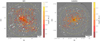 |
Fig. 1. View of the cluster members of Abell S1063 (left) and MACS J1206.2−0847 (right). The gray scale background image on the left (right) is the WFI (SUBARU) observation in the Rc band spanning an area of ≈25 × 25 arcmin2. The member galaxies are plotted as colored dots. The colors correspond to the stellar mass values of each galaxy as reported in the color bar. The three concentric yellow circles represent the distances of 1.5, 3, and 4.5 Mpc (1, 3, and 5 Mpc) from the cluster center identified with the BCG. The green rectangle represents the ≈1 × 2 arcmin2 (≈1 × 2.63 arcmin2) area covered by the MUSE spectroscopic follow-up on the inner regions of the cluster. |
2.1. Abell S1063 data
The cluster Abell S1063 (also known as RXC J2248.7−4431, labeled as AS1063) was first observed by Abell et al. (1989) and subsequently studied in detail as part of the CLASH and CLASH-VLT campaigns as well as by the Hubble Frontier Fields program of Lotz et al. (2017). AS1063 is a massive cluster (Sartoris et al. 2020 estimated a virial value of about 2 × 10¹⁵ M⊙) at redshift z = 0.35. Although the cluster has a regular shape, Gómez et al. (2012) and Rahaman et al. (2021) found from X-ray flux analyses that it may have recently undergone an off-axis merger. This hypothesis is challenged by the concentric distributions of the different mass components found by Bonamigo et al. (2018) (see also Beauchesne et al. 2023 for an independent X-ray and strong lensing analysis). The ICM in this cluster reaches temperature values of kBT ≈ 12 keV. AS1063 is an optimal gravitational lens that presents a set of 55 spectroscopically confirmed multiple images from 20 background sources distributed over a wide range of redshifts (0.73 < zsource < 6.11, see Caminha et al. 2016). The CLASH-VLT spectroscopic campaign yielded 3607 reliable redshifts, measured over a region of ≈25 × 25 arcmin2, 1109 of which are classified as cluster members according to techniques that use the projected phase-space distribution of galaxies around the median redshift value z = 0.3457 ± 0.0001 of the cluster (Mercurio et al. 2021). The catalog of cluster members and multiply lensed sources resulting from MUSE observations in the 1 × 2 arcmin2 central region was presented in Caminha et al. (2016), along with the first cluster strong lensing model. The full catalog was presented in Mercurio et al. (2021). The MUSE data provided 175 new secure redshifts, 104 of which are classified as cluster galaxies. By considering 21 additional redshifts from the literature (for more information about the data sample, see Sect. 2 in Sartoris et al. 2020), a total of 3850 spectroscopic redshifts were analyzed, and 1234 cluster members were selected for the dynamical analysis presented in that work (see also Mercurio et al. 2021). Additional photometric data, collected through the WFI, were necessary to measure the values of stellar mass of the cluster member galaxies from composite stellar population models. In the following analysis, we use the set of 1215 spectroscopically confirmed member galaxies with a stellar mass estimate. Following Mercurio et al. (2021), we inferred the stellar mass of the member galaxies from the information on the spectral energy distribution (SED) given by the available multiband photometry using composite stellar population models based on Bruzual & Charlot (2003) templates. The stellar mass values were estimated by assuming a Salpeter (1955) stellar Initial Mass Function (IMF), a delayed exponential star formation history, solar metallicity, and the presence of dust according to Calzetti et al. (2000). The radial completeness of our spectroscopic sample is discussed in Mercurio et al. (2021) and summarized in Table 1. The completeness of the sample is defined as the percentage of the cluster members with apparent magnitudes in the range 18.0 < mRc < 23.0, which were spectroscopically observed during the survey. The completeness decreases with the projected distance from the cluster center. In Appendix B, we test the robustness of our sample by running the same analysis on the subsample of cluster members with apparent magnitudes in the range 18.0 < mRc < 22.0.
Completeness of AS1063 spectroscopic sample.
2.2. MACS J1206.2−0847 data
The cluster MACS J1206.2−0847 (M1206, hereafter) was observed with the Hubble Space Telescope during the CLASH survey and then with the VLT/VIMOS as part of the CLASH-VLT program. The full redshift VIMOS catalog of MACS1206 consists of 3292 objects with measured redshifts mostly acquired as part of our ESO Large Programme 186.A-0798 (P.I.: Piero Rosati). Additional archival VIMOS data have been homogeneously reduced from programs 169.A-0595 (P.I.: Hans Böhringer) and 082.A-0922 (P.I. Mike Lerchster). M1206 is a massive galaxy cluster (Biviano et al. 2013 estimated a virial mass of 1.4 × 10¹⁵ M⊙) at redshift z = 0.4398 ± 0.0002 (Girardi et al. 2015). The cluster has a regular shape, presents a bright BCG, and its ICM has a temperature of kBT ≈ 11.6 keV (see Ebeling et al. 2009). A combined analysis of strong and weak lensing, X-ray surface brightness and temperature, and the Sunyaev-Zel’dovich effect (see Sereno et al. 2017 and Chiu et al. 2018) showed that the gas component of M1206 is remarkably regular and in hydrostatic equilibrium. M1206 is an excellent gravitational lens that presents 82 spectroscopic multiple images belonging to 27 families spanning the redshift range 1.0 < zsource < 6.1 (see Caminha et al. 2017). For this cluster, we merged two datasets taken from Biviano et al. (2013) and Caminha et al. (2017). Biviano et al. (2013) obtained a final catalog containing 2749 objects with reliable redshifts. Starting from this, the authors adopted a combination of two algorithms, the “Peak + Gap” method from Fadda et al. (1996) and the “Clean” method from Mamon et al. (2013), to identify the spectroscopic members of the cluster. They obtained a sample of 592 member galaxies (see also Annunziatella et al. 2014 for more information on this dataset). An additional 141 galaxies were observed with VLT/MUSE in the inner regions of the cluster and were spectroscopically confirmed as members of M1206 (see Caminha et al. 2017). By merging these two catalogs, we found that 44 members are in common between the two, thus bringing the final total number of member galaxies to 689. Photometric data in five bands (B, V, Rc, Ic, z′) obtained with SUBARU are available for 658 of the 689 spectroscopically confirmed members. We used this multiband photometric data to extend the catalog obtained in Annunziatella et al. (2014) that reports the stellar masses of 497 of these cluster members, adopting their fitting technique on the SED performed with the code MAGPHYS (da Cunha et al. 2008). This code is based on the stellar population synthesis models by Bruzual & Charlot (2003), with a Chabrier (2003) stellar IMF, a continuum star formation rate with superimposed random bursts, metallicity values between 0.02 and 2 solar, and the dust model of Charlot & Fall (2000). We converted the stellar mass values from a Chabrier to a Salpeter IMF (Madau & Dickinson 2014) to properly compare the stellar mass distributions of the two clusters. The completeness of the VIMOS sample is discussed in Biviano et al. (2013), while the galaxy sample observed with the MUSE instrument is approximately 100% complete in the magnitude range 18.0 < mRc < 23.0.
3. Basic properties of the galactic component
From the data presented in the previous section, we derived some basic properties of the galactic component of the two clusters, in particular, the line-of-sight velocity and stellar mass distributions. In addition, after a standard circularization, we derived the related surface number density and velocity dispersion profiles.
The velocity distributions for the two clusters are plotted in Fig. 2. The velocity distribution of AS1063 exhibits two peaks that are approximately 1000 km s−1 apart. The separation of the two peaks could indicate the presence of overall rotation or the existence of two different structures undergoing a merging phase; it might also just be an artifact related to the adopted binning. To test whether the two peaks in the velocity distribution of AS1063 are related to a bimodal distribution, we performed the so-called dip test developed by Hartigan & Hartigan (1985), which measures unimodality in a sample by the maximum difference over all sample points between the empirical distribution function and the unimodal distribution function that minimizes that maximum difference. The dip test gave a p-value of 0.976, suggesting that the distribution is compatible with a single Gaussian distribution. Other tests would thus be required to study the possible presence of rotation (see Sect. 4) or merging. Furthermore, the dip test encourages us to consider the standard deviation of a Gaussian as a good choice for the global velocity dispersion, even for the case of AS1063, which is apparently associated with a two-peaked velocity distribution profile. The velocity dispersions for AS1063 and M1206 are 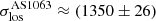 km s−1 and
 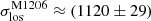 km s−1, respectively. For AS1063, Mercurio et al. (2021) obtained a velocity dispersion value of
  km s−1, which is compatible with our estimate. For M1206, Girardi et al. (2015) obtained a velocity dispersion value of
  km s−1, which is lower than our result. The difference can be explained by the inclusion of 97 additional sources in our catalog that were detected with VLT/MUSE (Caminha et al. 2017) in the inner regions of the cluster, as mentioned in Sect. 2.
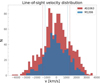 |
Fig. 2. Line-of-sight velocity distribution for the member galaxies of the two clusters. The vertical dashed lines represent the corresponding velocity dispersion σlos. The binning procedure consisted of dividing the range of observed line-of-sight velocities in bins of 200 km s−1. |
The stellar mass distributions are plotted in Fig. 3. The distributions underestimate the number of low-mass galaxies because of the observational limits in apparent magnitudes characterizing the sample.
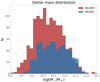 |
Fig. 3. Stellar mass distribution for the two clusters divided into bins of 0.15 dex. Because the individual galaxies also contain DM halos and gas, the total mass distribution would be shifted to the right of the diagram and would possibly have a different shape. |
A preliminary step required in calculating the number density and line-of-sight velocity dispersion profile is to define the cluster center. For the two clusters, the distributions of galaxies, hot ICM, and DM are almost concentric (see Bonamigo et al. 2018, who found that the corresponding centers are within ≈10 kpc from one another and that they basically coincide with the center of the cluster BCG). This is why we chose the position of their BCGs in the sky as the center of the two clusters, as they are well constrained by the available photometric data. The fact that the three main mass components are almost concentric provides strong observational evidence that the clusters have reached a well-defined quasi-equilibrium state.
For simplicity, we assumed that the galactic projected number density distribution in the two clusters has contour levels described by confocal ellipses with constant eccentricity, defined in terms of the major and minor semi-axes a and b as 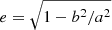 . The eccentricities of the two clusters are listed in Table 2. By converting these values into ellipticities (ε = 1 − b/a), we note that the flattening that is involved is similar to that of E3-E4 elliptical galaxies. We recall that the eccentricity of a discrete distribution of points can be found from the second moments of such distribution (for the derivation and an application to galaxy clusters, see de Theije et al. 1995). Then, in constructing the number density and velocity dispersion profiles, we referred to the circularized radius
  , in which the projected distance of a galaxy from the cluster center is defined in terms of the major and minor semi-axes of the isodensity contour on which the galaxy is located.
Structural properties of the two clusters.
The plots provided in Figs. 4 and 5 are profiles expressed as a function of the dimensionless radius R/Rhm. Here, the half-mass radius Rhm is defined as the (circularized) radius that encloses half of the stellar mass projected on the sky. Remarkably, in this representation, the surface number density and velocity dispersion profiles of the two clusters basically overlap out to approximately 3 Rhm.
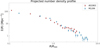 |
Fig. 4. Projected number density profile of the galactic component as a function of the radial distance from the cluster center. For each cluster, the circularized radius R was measured in terms of the half-mass radius defined on the basis of its stellar mass distribution. The bins were obtained by dividing the range of observed R/Rhm of each cluster into 20 subintervals. The error bars are 1σ. As briefly described in the text, the profiles are affected by the sample incompleteness in a nontrivial way. |
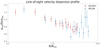 |
Fig. 5. Line-of-sight velocity dispersion profile of the galactic component as a function of the radial distance from the cluster center normalized to the global velocity dispersion σlos of each cluster. As in Fig. 4, for each cluster, the circularized radius R was measured in terms of the cluster stellar half-mass radius, and the bins were defined according to the same procedure. The vertical bars represent the errors evaluated as |
Figure 4 illustrates the surface number density profiles. The observed surface number density can be approximated by a monotonically declining power law, at least out to ≈3Rhm, with the exponent ≈1.5. This is consistent with the findings of Biviano et al. (2013) for M1206 (see Fig. 7 of that paper) and of Sartoris et al. (2020) for AS1063 (see Fig. 3 of that paper). Figure 5 shows the velocity dispersion profiles. The value of the velocity dispersion in each radial bin was normalized to the global velocity dispersion of the cluster considered. This is also consistent with the velocity dispersion profile found by Biviano et al. (2013) for M1206 (see Fig. 3 of that paper).
In the cosmological context, a commonly used scale for the radius of a cluster is the so-called virial radius, generally denoted as r200. We note that the ratio of r200 to Rhm for the two clusters is in the range of 1.1 − 1.6 (see Table 2). Therefore, we can state that the similarities between the radial profiles of the two clusters represented in Figs. 4 and 5 hold out to about 2 − 3 virial radii.
Figure 5 shows that both clusters display a regular, monotonically decreasing velocity dispersion profile within 3 half-mass (i.e., ≈2 virial) radii. This regularity seems to be in contradiction with a possible recent merger in AS1063 (Gómez et al. 2012; Rahaman et al. 2021; Mercurio et al. 2021; Beauchesne et al. 2023). The kinematic data on the cluster members of M1206 extend beyond this point, and it appears that the decreasing trend is interrupted, which may be interpreted as an indication that in those outer regions, the cluster has not yet reached a quasi-equilibrium state.
In Table 2, we report an estimate of the relaxation time TD for the two clusters considered in this paper based on the definition (see Chandrasekhar 1941)
 (1)
(1)
where we have taken the standard estimate lnΛ ≈ 10, and for σ, n, and m, we have inserted the values obtained from the previous data by applying the following definitions: σ = σlos is the global velocity dispersion, and m is the typical mass of a galaxy (taken to be the mean value of the stellar mass distribution in Fig. 3, ignoring the DM halo and gas contribution to the total mass budget of a single galaxy, which are expected to be greater than the stellar mass alone by a factor of about two to three). The average number n density used to obtain the relaxation time was derived from a power law fit on the measured surface number density (the average was performed within the radial interval [0.1, 1] half-mass radii). By comparing these values to those of the crossing time 2Rhm/σlos ≈ 2 Gyr and to the Hubble time, we thus confirmed the common picture that the galactic component in clusters should be considered as collisionless (see for example Sarazin 1988).
4. Search for the presence of mean rotation
In the previous section, we noted that the spatial distribution of galaxies in the two clusters is flattened, similar to E3-E4 galaxies. The principal axes of the galaxy distributions are aligned with those of the central BCG. In addition, the ICM and DM, as from X-ray and gravitational lensing analyses, are also characterized by flat spatial distributions aligned with the galactic component (Bonamigo et al. 2018). If rotation is responsible for the observed flattening, gradients in the line-of-sight galaxy velocity distribution would be expected along the major axes, and negligible gradients should be found along the minor axes. In addition, as a reference value, we refer to the (V/σ, ε) diagram in Fig. 1 of the article by Davies (1987), which suggests that for E3-E4 oblate isotropic rotators (following the very simple picture of the homogeneous self-gravitating classical ellipsoids, as in Chandrasekhar 1969), the expected ratio of peak rotation velocity |vrot| to velocity dispersion should be approximately 0.7 (and ≈0.4 for prolate rotators). The quantity V/σ is the ratio of the observed maximum of the rotation profile to the line-of-sight velocity dispersion.
As an initial simple test of the possible presence of rotation related to the observed flattening in the galactic component of AS1063 and M1206, we divided each cluster into four sectors in relation to its major and minor axes and then plotted the line-of-sight velocity distribution for the galaxies inside each sector. The sectors and the galaxy subsamples for the two clusters were defined in the following way: member galaxies with a projected distance from the cluster center R < Rhm are divided into four circular sectors and grouped according to their closest principal axis, whereas galaxies with R > Rhm are added to a sector if they are within a distance  from the closest principal axis. These sectors are highlighted in Fig. 6 for M1206. For each cluster the line-of-sight velocities are the internal velocities obtained after subtraction of the mean velocity of the full sample of galaxies, as in Fig. 2. The results for M1206 are illustrated in Fig. 7, and some quantitative results for the two clusters are recorded in Table 3. We produced position–velocity diagrams for the cluster members found within a distance D < (1/2)Rhm from the major and minor axis, as shown in Fig. 8. As summarized in Figs. 7 and 8, both tests suggest that there is little or no evidence for internal rotation, neither oblate nor prolate (of the kind discussed in Ebrová & Łokas 2017), in the galactic component of the two clusters when considering the whole samples.
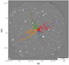 |
Fig. 6. Sample of member galaxies divided into sectors along the major (blue line) and minor (red line) axes for M1206 following the steps introduced in Sect. 4. The dashed yellow circle represents the half-mass radius Rhm. The sectors are identified as sector A in blue, sector B in orange, sector C in green, and sector D in red. If rotation were responsible for the observed flattening, gradients in the line-of-sight galaxy velocity distribution would be expected along the major axes and not along the minor axes. |
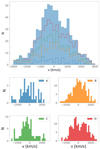 |
Fig. 7. Distribution of the line-of-sight velocities of member galaxies of M1206 contained in the sectors shown in Fig. 6. Upper histogram: stacked distribution of velocities in the four sectors compared to the total velocity distribution of Fig. 2. Lower histograms: velocity distributions of the galaxies in each sector. The sectors are identified as sector A in blue, sector B in orange, sector C in green, and sector D in red. |
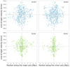 |
Fig. 8. Position-velocity diagrams of the member galaxies within a distance D < (1/2)Rhm from the major (left) and minor (right) axes of AS1063 (cyan) and M1206 (green). These plots do not show any clear rotation signature (which would offset the points in the diagrams toward two diagonally opposite quadrants). |
Summary of the mean velocities ⟨v⟩sec and velocity dispersion σlos,sec inside each sector.
We should emphasize that the (V/σ, ε) relation involves only global quantities (Binney 1978, Binney 2005). The diagram shown in Davies (1987) should be significantly modified to include inclination effects and the change in pressure anisotropy with radius (Cappellari et al. 2007). In addition, some self-gravitating stellar systems exhibit clear evidence of solid-body rotation only in their innermost regions (e.g., see Bianchini et al. 2013; Leanza et al. 2023).
To check whether the clusters have an isotropic (or mildly anisotropic) core characterized by significant mean rotation, we derived the rotation profile for the galaxies within a circular region of 0.5′ radius from the center of each cluster (i.e., within the MUSE pointings) by maximizing the number of galaxies considered and thus avoiding a potentially sharp variation of the sample completeness that occurs at larger radii.
We first identified the angle (PA) of the projected rotation axis in the plane of the sky (defined as the angle between the rotation axis and the right ascension axis). To identify the value of PA, we followed a standard procedure in globular cluster studies (e.g., see Cote et al. 1995; Bianchini et al. 2013; Leanza et al. 2023): we computed the mean line-of-sight velocities in the two subsamples obtained by dividing the cluster members by a line passing through the cluster center with a given PA. The PA was varied in steps of 10 deg, and the difference between the mean velocities ΔVmean was plotted against the PA. The resulting pattern was fitted with a sine function. The PA at which the maximum difference in mean velocities was reached corresponds to the (projected) rotation axis, and the amplitude of the sine function is twice the rotation amplitude V. If the clusters are characterized by the presence of mean rotation, the position-velocity diagrams would show an asymmetry, and the galaxies on each side of the rotation axis would be expected to be sampled from distinct cumulative velocity distributions. The results of this analysis are plotted in Fig. 9.
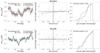 |
Fig. 9. Diagnostic diagrams of the rotation signature detected in the core of the two clusters within 0.5′ from the center. This corresponds to the areas covered by the MUSE pointings. The left panels show the difference between the mean velocities ΔVmean on each side of a line passing through the center with the given angle (PA) divided by the velocity dispersion |


Figure 9 indicates that in the core of both clusters there is significant evidence of rotation (V/σ ≈ 0.15). The minor axis of the galaxy distribution in the core is offset by 30 deg from the best-fit rotation axis. The eccentricity (ellipticity) of AS1063 and M1206 within 0.5′ from their centers is e = 0.60 (ε = 0.2) and e = 0.77 (ε = 0.37), respectively. The ratio of peak rotation velocity to velocity dispersion required to sustain an edge-on oblate isotropic rotator with the ellipticity of AS1063 (M1206) would be V/σ ≈ 0.4 (≈0.6). However, by relaxing the condition on isotropy, the ratio of V/σ required to maintain an oblate shape is lowered (Cappellari et al. 2007). For example, a mild anisotropy (this concept and the related definition are properly introduced in Sect. 6.2) of β ≈ 0.15 would be compatible with the requirement of an oblate rotator with the shape of the core of AS1063.
A prolate rotator (of the kind studied in Binney 1978) would require a lower amount of pressure anisotropy to sustain the observed eccentricity of the cores. However, it would introduce serious modeling complications, as the rotation axis is perpendicular to the symmetry axis. Thus, the component of the specific angular momentum along the rotation axis is not an integral of the motion.
As further confirmation of a rotating core, we note that Fig. 22 in Sereno et al. (2017) shows a drop in the ratio of thermal and nonthermal pressure (possibly related to the presence of bulk motions, see Meneghetti et al. 2010) in the inner approximately 100 kpc h−1 of M1206, which corresponds exactly with the region within 5 arcmin from the cluster center where we detected the presence of mean rotation.
In Appendix C, we apply the analysis discussed in this subsection to the whole sample and to the galaxies within 5 arcmin, confirming the absence of rotation at large radii. As a side note, a test for rigid rotation similar to that considered by Hwang & Lee (2007) failed to give a clear signal of rotation in the center for these two clusters (because of the low signal-to-noise ratio of the mean rotational motion), while it correctly indicated the absence of rotation at large radii.
5. Empirical evidence of the absence of collisional relaxation
In relaxed thermodynamical (i.e., collisional) systems, two properties are expected to be established independently of the initial conditions: energy equipartition, that is, the velocity dispersion of particles of mass m should scale as m−1/2, and mass segregation, that is, lighter particles should be characterized by a more diffuse distribution than that of heavier particles (e.g., see Smith 1936; Spitzer 1987).
To look for hints of mass segregation, we divided the galactic component in mass bins based on the galaxy stellar mass M⋆. We then studied the ratio of the half-mass radius measured based on the subdistribution of galaxies associated with each bin to the global half-mass radius Rhm as a function of M⋆. As shown in Fig. 10, we observed that a decreasing trend for Rhm(M⋆) is indeed present in both clusters, though it is more pronounced in M1206. Therefore, both clusters appear to be mass segregated, relative to the stellar mass. Of course, in terms of total mass, mass segregation is likely to be associated with a profile different from that of Fig. 10. Furthermore, the characteristics of the profiles illustrated in Fig. 10 need not result from the slow action of collisionality and can instead be from different evolutionary processes, such as galaxy merging. At first glance, our results might seem at odds with those of Biviano et al. (2013), who found that the concentration of the luminosity density is around 10% higher than the concentration of the luminosity density, reporting little evidence for mass segregation. This cumulative approach ignores the stellar mass distribution shown in Fig. 3. Massive galaxies are less common and therefore can be segregated and still give a relatively small contribution to the overall concentration.
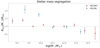 |
Fig. 10. Evidence of mass segregation. The galaxies were divided into bins according to their stellar mass. This plot shows the variation of Rhm(M⋆), which is the half-mass radius of the cluster members inside the nth bin normalized to the global half-mass radius, with galactic mass. The errors were evaluated as |

In any case, mass segregation poses a contradiction to the simple use of one-component models in the interpretation of the observations. This point has already been addressed for M1206 by Biviano et al. (2013), who considered the populations of passive and star-forming galaxies separately (which roughly correspond to elliptical and spirals, respectively). In a different physical context, to take into account the possible presence of mass segregation, two-component models have also been considered in the literature to describe globular clusters (for example, see de Vita et al. 2016; Torniamenti et al. 2019).
In Fig. 11, we compare the velocity dispersion for galaxies with different stellar masses, adopting the same binning procedure as the one used in Fig. 10. The plot suggests that AS1063 and M1206 do not exhibit evidence of energy equipartition. Further analyses focusing only on the central regions (R < (1/5) Rhm) confirmed the absence of energy equipartition.
 |
Fig. 11. Absence of energy equipartition. The galaxies are divided in bins according to their stellar mass. This plot shows the variation of σlos(M⋆), which is the velocity dispersion of the cluster members inside the nth bin normalized to the global velocity dispersion, with galactic mass. The errors were evaluated as |


The absence of equipartition, in spite of the presence of some mass segregation, supports the argument that the galactic component in each of the two clusters should be considered a collisionless component and that the origin of mass segregation should reflect some evolutionary process in the formation of the two clusters unrelated to galaxy–galaxy scattering.
6. Dynamical models
6.1. Number density from the observations
In the next subsection, we will apply the Jeans equations to make dynamical predictions for the velocity dispersion profiles, testing different hypotheses on the velocity dispersion anisotropy present in the two clusters. To do so, we assumed that the number density of galaxies is known (from the available number counts) and that the overall potential well is also known (from published gravitational lensing investigations). In the context of stellar dynamics, spherically symmetric models have often proved successful in describing astrophysical objects with a wide variety of apparent morphologies (e.g., see Saglia et al. 1992 Sect. 3.2, in particular Fig. 1, for a test on the effectiveness of spherical models on strongly flattened – E4/E6 – elliptical galaxies). On the other hand, the task of trying to take into account the dynamical effects of flattening or triaxiality would be nontrivial, and the enormous complexity required in such modeling would not be sufficiently justified by the available data.
For simplicity, we developed our models under the assumption that each cluster is spherically symmetric.
In this context, one key step is the derivation of the volume (three-dimensional) number density n(r) starting from the surface (projected) number density Σ(R) of the galactic component of the two clusters1:
 (2)
(2)
where r is the three-dimensional radius and R is the radius projected on the sky surface. Deriving the volume number density from the projected density Σ(R) corresponds to the classical problem known as Abel inversion. Here, we preferred to work on the direct problem, starting from three well-known spherically symmetric analytical power law volume density profiles, namely, the Jaffe (1983) profile, the Navarro–Frenk–White (NFW) profile (see Navarro et al. 1997), and the spherical limit of the dual Pseudo Isothermal Ellipsoid (dPIE, see Kassiola & Kovner 1993). These profiles depend on two scales (two scales and one dimensionless parameter for the dPIE): a density scale and a length scale.
The Jaffe number density profile is
 (3)
(3)
The NFW number density profile is
 (4)
(4)
The dPIE number density profile is
![Mathematical equation: $$ \begin{aligned} n_{\rm dPIE}(r) = \frac{ n_0}{[1+(r/r_{\rm core})^2][1+(r/r_{\rm cut})^2]} ,\end{aligned} $$](/articles/aa/full_html/2023/08/aa46226-23/aa46226-23-eq21.gif) (5)
(5)
with rcut > rcore.
The Jaffe profile was developed in the context of the dynamics of elliptical galaxies. Close to the origin, it approaches the profile of a singular isothermal sphere, and at large radii, it is characterized by a decline that guarantees a finite total number of particles. The NFW profile is often adopted in the cosmological context because numerical simulations on the growth of DM halos appear to be well modeled by this profile. The dPIE profile is mostly used in gravitational lensing studies to model the total mass distribution of a lens because of its convenient analytical properties: It is approximately constant below rcore and scales approximately as n(r)∼r−2 in the radial range rcore < r < rcut. These profiles admit a simple analytical expression for the projected density profile, that is, for the integral of Eq. (2) (for an example, see Ciotti et al. 2019 for the Jaffe profile and Limousin et al. 2005 for the dPIE and NFW profiles).
We fitted the observed projected number density profiles shown in Fig. 4 using these simple models. For the cluster AS1063, the results are illustrated in Fig. 12 and show that the three models all fit the available photometric data reasonably well.
 |
Fig. 12. Observed surface number density of AS1063 (in green) fitted with the projected Jaffe, dPIE, and NFW profiles (in red). Top row: profiles resulting from the best-fit process. Bottom row: fractional deviations between the analytical model and the photometric data. The labels provide the reduced χ2 values. |
6.2. Jeans equations
Under different assumptions of the local anisotropy profile, β(r) is defined as a function of the diagonal elements of the velocity dispersion tensor σii:
 (6)
(6)
We tested whether the Jeans equations (for assigned galaxy number density profile and total gravitational field in the two clusters AS1063 and M1206) predict line-of-sight velocity profiles for the galactic component compatible with the observations. For simplicity, the analysis was carried out under the assumption of spherical symmetry, absence of mean rotation, and proportionality between number and mass density for the galactic component. The relevant (radial) equation can be written as
 (7)
(7)
The boundary condition adopted to solve this differential equation is defined at large radii, where the velocity dispersion σrr(r) is assumed to vanish. bIn the context of clusters of galaxies, the function M(r) is the total mass enclosed in a sphere of radius r dominated by the contributions of DM and the ICM. bFor this reason, we refer to the final models based on strong- and weak-gravitational lensing described in Umetsu et al. (2016) (see Table 4). The total mass profile for an NFW model expressed as a function of the parameters listed in Table 4 is
 (8)
(8)
Cluster parameters derived for the total mass distribution described by a spherical NFW model reconstructed from combined strong-lensing, weak-lensing shear and magnification measurements.
The number density profiles are from the analysis of Sect. 6.1. In the following analysis, we refer only to the representation in terms of a Jaffe profile. The choice of a Jaffe profile was motivated by its regular properties (i.e., finite total mass). In Appendix D, we show the results of the Jeans analysis using an NFW number density profile, which turned out to be very similar bto the outcomes of this section.
By projecting the solution for the radial velocity dispersion, we obtained
 (9)
(9)
for the predicted velocity dispersion along the line of sight (the integration we implemented follows Appendix 2 of Mamon & Łokas 2005). For the local anisotropy profile, we decided to take the following three-parameter function:
 (10)
(10)
The function β(r) thus exhibits an isotropic (i.e., β = 0) center and may be either radially (β > 0) or tangentially (β < 0) biased at large radii (r > rβ). The set of parameters considered in our analysis are listed in Table 5.
Distribution function parameters.
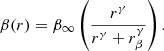
The results of the Jeans equation approach are illustrated in Fig. 13. For an easier reading, it shows the velocity dispersion profiles associated only with two choices of β(r), the isotropic (β∞ = 0, rβ = 0) and the so-called Osipkov–Merritt profile (β∞ = 1, γ = 2). While the confidence regions of both solutions can reproduce the kinematical data reasonably well, it is clear that the decreasing trend of the observed velocity dispersion profile is better represented in the solution associated with the Osipkov–Merritt anisotropy profile (in particular within 3 Mpc, which is the range within which the gravitational field was obtained by Umetsu et al. 2016). This result is consistent with other results present in the literature, especially in the work by Biviano et al. (2013) on M1206 (in particular, see Fig. 14 of this article) and by Sartoris et al. (2020) on AS1063 (see Table 1 of this article). The velocity dispersion anisotropy profiles suggest the presence of a mild anisotropy in the core (β(0.5′) ≈ 0.05) slightly less than the quantity required to justify the shape of the core.
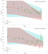 |
Fig. 13. Line-of-sight velocity dispersion profile of the galactic component obtained from the Jeans equation for AS1063 and M1206. The plots show the data points (in green) derived from the spectroscopic data (see Fig. 5) superimposed on the velocity profiles derived from the Jeans equation for two choices of β(r): the constant isotropic β = 0 profile (in cyan) and the Osipkov–Merritt anisotropy profile (in red). The confidence regions were found by allowing the total mass M(r) to vary within the uncertainties of the values of its parameters reported in Table 4. The confidence levels were underestimated for R > 3 Mpc because, in this region, the total mass M(r) is extrapolated and not directly constrained by the observations. |
6.3. A dynamical model based on a physically justified distribution function
In this last subsection, we explore the possibility that the galactic component might be described by a distribution function of the form that was originally conceived to incorporate formation by incomplete violent relaxation (in particular, see Stiavelli & Bertin 1987; Bertin & Trenti 2003; Trenti & Bertin 2005). In the context of the dynamics of individual elliptical galaxies, the function has been successfully used to model the observations in not only the one-component case for galaxies in which DM appears to be lacking (as is the case of NGC 3379; see Saglia et al. 1992; Bertin & Stiavelli 1993; Romanowsky et al. 2003) but also in self-consistent two-component models for galaxies in which evidence of the presence of DM is significant (as is the case of NGC 4472; see Saglia et al. 1992). In this paper, we explore the use of this distribution function in a completely different situation, that is, the case in which the component described by the distribution function (i.e., the galaxies of the two clusters) does not contribute significantly to the total gravitational field in which it is embedded. In other words, the mean gravitational potential that will appear in the distribution function is assumed to be an external potential due entirely to the ICM and DM components.
The distribution function that we considered is (see Stiavelli & Bertin 1987; with ν = 1)
 (11)
(11)
where the specific energy E and the specific angular momentum J are defined as E = v2/2 + Φ(r) and J = |r × v|. In the fully self-consistent case in which the “particles” described by the distribution function determine the mean gravitational potential, the boundary conditions to the Poisson equation impose a relation between the depth of the potential well Φ(0) and a dimensionless parameter that depends on A, a, and d. In the contexr of clusters of galaxies, the mean potential is external and imposed – in our model, we refer to the total mass profile described by Umetsu et al. (2016) and introduced in Sect. 6.2. Therefore, the three (positive) parameters can be adjusted independently to produce a best-fit to the available data for the galactic component assumed to be described by the above distribution function. The parameter A sets the scale of the density profile, whereas parameter a sets the scale of the velocity dispersion profile. The third parameter, d, can be adjusted to determine the radius beyond which the velocity dispersion is significantly anisotropic.
The relevant calculations are best carried out after a suitable reduction to dimensionless variables. In particular, we defined the imposed dimensionless potential as ψ = −aΦ and referred to the dimensionless radial coordinate x = r/rs, where for each cluster rs is the scale of the best-fit NFW potential of Table 4 so that ψ(x) = Ψx−1ln(1 + x). By inserting the imposed potential in Eq. (11), it is possible to compute the volume density n(r), the radial velocity dispersion σrr(r), and the local anisotropy profile β(r) from the distribution function. By suitable integration, these profiles can be converted into projected profiles Σ(R) and σlos(R) and compared with the observations. For each cluster, this procedure led to the determination of the best-fit parameters A, a.
In Figs. 14 and 15 we observed how the line-of-sight velocity dispersion parameter and projected number density profiles vary as a function of d. We note that the parameter range d = 10 − 50 leads to a self-consistent dynamical model that matches the photometric and spectroscopic observations and is characterized by isotropic pressure in the center and radial pressure anisotropy in the outer regions (see Fig. 16), as also indicated by the results based on the Jeans equations in the previous subsection.
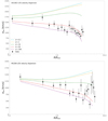 |
Fig. 14. Line-of-sight velocity dispersion profile of the galactic component derived from the f(ν) distribution function with fitted parameters for AS1063 and M1206 (see Table 6). The plot shows the data points (in black) derived from spectroscopic data (see Fig. 5) superimposed on the velocity profiles derived from the moments of the distribution function for five choices of the value of the parameter d (see Fig. 16 for the associated anisotropy profile). Both clusters are well described by the velocity dispersion curves associated with a value of d ≈ 10 − 50. |
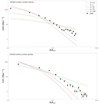 |
Fig. 15. Projected number density profile of the galactic component derived from the f(ν) distribution function with fitted parameters for AS1063 and M1206 (see Table 6). The plot shows the data points (in black) derived from photometric data (see Fig. 4) superimposed on the projected number density profile derived from the moments of the distribution function for five choices of the value of the parameter d (see Fig. 16 for the associated anisotropy profile). The value of the parameter A was obtained after a best-fit against the observed profile performed within 2Rhm. Both clusters are well described by the curves associated with a value of d ≈ 10 − 50, confirming the results of Fig. 14. |
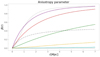 |
Fig. 16. Anisotropy parameter radial profile. The colored solid lines show the anisotropy profile as a function of the free parameter d. The distribution of the stellar orbits associated with the adopted distribution function is characterized by isotropy in the central region and radially biased anisotropy in the outer parts, which becomes more prominent as the value of d increases. The dashed, dashed-dotted, and dotted gray curves represent, respectively, the isotropic, radial, and Osipkov–Merritt anisotropy profiles of Table 5. |
The velocity dispersion anisotropy profiles with d = 10 − 50 suggest the presence of mild anisotropy in the core β(0.5′) ≈ 0.05. If the measurements of the anisotropy profiles are accurate in the very central regions, we may argue that the cores do not follow the standard (V/σ, ε) relation mentioned in Sect. 4.
For a detailed description, see Appendix A. In Appendix B, we test the robustness of our sample by imposing a cut in magnitude at mRc ≤ 22.
7. Conclusions
In this paper, we investigated some dynamical properties of the galactic components of two clusters of galaxies: Abell S1063 and MACS J1206. In particular, we addressed the question of the possible presence of systematic rotation and the issue of their general relaxation state. We found evidence for differential rotation in both clusters, with slow rotation (Vr/σ ≈ 0.15) in the centers tapering off at larger radii and pressure anisotropy. Differential rotation and pressure anisotropy can contribute to produce nontrivial gradients in the phase space. Therefore, it would be useful to extend this study to more complex dynamical models (for an example developed for globular clusters, see Varri & Bertin 2012). It would be interesting to check whether the ICM component of these two clusters is also characterized by a lack of systematic rotation. Notably, an X-ray measurement of this property is likely to become available in the near future (see Bianconi et al. 2013; Liu & Tozzi 2019).
As to the relaxation state of the two clusters, no signs were found of energy equipartition, but there is a clear indication of (stellar) mass segregation. The presence of mass segregation in the absence of equipartition suggests that the observed mass segregation is associated with mechanisms that are unrelated to the possible role of collisional processes (galaxy–galaxy encounters).
Indeed, velocity dispersion anisotropy was found to be present in the two clusters and turns out to be qualitatively similar to what has been found in violently relaxed collisionless systems (see Sect. 6.2). This last conclusion is strengthened by the overall success in matching the observations with the predictions of a physically justified distribution function with an imposed external potential, as described in Sect. 6.3.
Given the incomplete information available on the galaxy mass distribution for the two clusters, we refer to the number density n instead of the mass density ρ.
Acknowledgments
We thank the anonymous referee for useful comments that improved the presentation. We acknowledge financial support through grants PRIN-MIUR 2017WSCC32 and 2020SKSTHZ, and INAF “main-stream” 1.05.01.86.20 and 1.05.01.86.31.
References
- Abell, G. O., Corwin, H. G., Jr, & Olowin, R. P. 1989, ApJS, 70, 1 [Google Scholar]
- Annunziatella, M., Biviano, A., Mercurio, A., et al. 2014, A&A, 571, A80 [NASA ADS] [CrossRef] [EDP Sciences] [Google Scholar]
- Baade, D., Meisenheimer, K., Iwert, O., et al. 1999, The Messenger, 95, 15 [NASA ADS] [Google Scholar]
- Bacon, R., Accardo, M., Adjali, L., et al. 2010, in Ground-based and Airborne Instrumentation for Astronomy III, eds. I. S. McLean, S. K. Ramsay, & H. Takami, SPIE Conf. Ser., 7735, 773508 [Google Scholar]
- Bahcall, N. A. 1977, ARA&A, 15, 505 [Google Scholar]
- Bailin, J., & Steinmetz, M. 2005, ApJ, 627, 647 [Google Scholar]
- Bautz, L. P., & Morgan, W. W. 1970, ApJ, 162, L149 [NASA ADS] [CrossRef] [Google Scholar]
- Beauchesne, B., Clément, B., Hibon, P., et al. 2023, MNRAS, submitted [arXiv:2301.10907] [Google Scholar]
- Bertin, G. 2014, Dynamics of Galaxies, 2nd edn. (Cambridge: Cambridge University Press) [Google Scholar]
- Bertin, G., & Stiavelli, M. 1993, Rep. Progr. Phys., 56, 493 [CrossRef] [Google Scholar]
- Bertin, G., & Trenti, M. 2003, ApJ, 584, 729 [NASA ADS] [CrossRef] [Google Scholar]
- Bianchini, P., Varri, A. L., Bertin, G., & Zocchi, A. 2013, ApJ, 772, 67 [NASA ADS] [CrossRef] [Google Scholar]
- Bianconi, M., Ettori, S., & Nipoti, C. 2013, MNRAS, 434, 1565 [NASA ADS] [CrossRef] [Google Scholar]
- Binney, J. 1978, MNRAS, 183, 501 [NASA ADS] [Google Scholar]
- Binney, J. 2005, MNRAS, 363, 937 [Google Scholar]
- Biviano, A., Rosati, P., Balestra, I., et al. 2013, A&A, 558, A1 [Google Scholar]
- Bonamigo, M., Grillo, C., Ettori, S., et al. 2018, ApJ, 864, 98 [Google Scholar]
- Bruzual, G., & Charlot, S. 2003, MNRAS, 344, 1000 [NASA ADS] [CrossRef] [Google Scholar]
- Buote, D. A., & Canizares, C. R. 1992, ApJ, 400, 385 [NASA ADS] [CrossRef] [Google Scholar]
- Buote, D. A., & Canizares, C. R. 1994, ApJ, 427, 86 [NASA ADS] [CrossRef] [Google Scholar]
- Buote, D. A., Jeltema, T. E., Canizares, C. R., & Garmire, G. P. 2002, ApJ, 577, 183 [CrossRef] [Google Scholar]
- Calzetti, D., Tremonti, C. A., Heckman, T. M., & Leitherer, C. 2000, in Massive Stellar Clusters, eds. A. Lançon, & C. M. Boily, ASP Conf. Ser., 211, 25 [NASA ADS] [Google Scholar]
- Caminha, G. B., Grillo, C., Rosati, P., et al. 2016, A&A, 587, A80 [NASA ADS] [CrossRef] [EDP Sciences] [Google Scholar]
- Caminha, G. B., Grillo, C., Rosati, P., et al. 2017, A&A, 607, A93 [NASA ADS] [CrossRef] [EDP Sciences] [Google Scholar]
- Cappellari, M., Emsellem, E., Bacon, R., et al. 2007, MNRAS, 379, 418 [Google Scholar]
- Chabrier, G. 2003, PASP, 115, 763 [Google Scholar]
- Chandrasekhar, S. 1941, ApJ, 93, 285 [NASA ADS] [CrossRef] [Google Scholar]
- Chandrasekhar, S. 1969, Ellipsoidal Figures of Equilibrium (New Haven: Yale University) [Google Scholar]
- Charlot, S., & Fall, S. M. 2000, ApJ, 539, 718 [Google Scholar]
- Chiu, I. N., Umetsu, K., Sereno, M., et al. 2018, ApJ, 860, 126 [NASA ADS] [CrossRef] [Google Scholar]
- Ciotti, L., Mancino, A., & Pellegrini, S. 2019, MNRAS, 490, 2656 [NASA ADS] [CrossRef] [Google Scholar]
- Cote, P., Welch, D. L., Fischer, P., & Gebhardt, K. 1995, ApJ, 454, 788 [NASA ADS] [CrossRef] [Google Scholar]
- da Cunha, E., Charlot, S., & Elbaz, D. 2008, MNRAS, 388, 1595 [Google Scholar]
- Davies, R. L. 1987, in Structure and Dynamics of Elliptical Galaxies, ed. P. T. de Zeeuw, 127, 63 [NASA ADS] [CrossRef] [Google Scholar]
- de Theije, P. A. M., Katgert, P., & van Kampen, E. 1995, MNRAS, 273, 30 [NASA ADS] [Google Scholar]
- de Vita, R., Bertin, G., & Zocchi, A. 2016, A&A, 590, A16 [NASA ADS] [CrossRef] [EDP Sciences] [Google Scholar]
- Dressler, A. 1981, ApJ, 243, 26 [NASA ADS] [CrossRef] [Google Scholar]
- Ebeling, H., Ma, C. J., Kneib, J. P., et al. 2009, MNRAS, 395, 1213 [Google Scholar]
- Ebrová, I., & Łokas, E. L. 2017, ApJ, 850, 144 [Google Scholar]
- Fadda, D., Girardi, M., Giuricin, G., Mardirossian, F., & Mezzetti, M. 1996, ApJ, 473, 670 [NASA ADS] [CrossRef] [Google Scholar]
- Girardi, M., Mercurio, A., Balestra, I., et al. 2015, A&A, 579, A4 [NASA ADS] [CrossRef] [EDP Sciences] [Google Scholar]
- Gómez, P. L., Valkonen, L. E., Romer, A. K., et al. 2012, AJ, 144, 79 [CrossRef] [Google Scholar]
- Gregory, S. A., & Tifft, W. G. 1975, Bull. Am. Astron. Soc., 7, 539 [Google Scholar]
- Hartigan, J. A., & Hartigan, P. M. 1985, Ann. Stat., 13, 70 [Google Scholar]
- Humphrey, P. J., Buote, D. A., Canizares, C. R., Fabian, A. C., & Miller, J. M. 2011, ApJ, 729, 53 [CrossRef] [Google Scholar]
- Hwang, H. S., & Lee, M. G. 2007, ApJ, 662, 236 [NASA ADS] [CrossRef] [Google Scholar]
- Jaffe, W. 1983, MNRAS, 202, 995 [NASA ADS] [Google Scholar]
- Kassiola, A., & Kovner, I. 1993, ApJ, 417, 450 [Google Scholar]
- Kravtsov, A. V., & Borgani, S. 2012, ARA&A, 50, 353 [Google Scholar]
- Leanza, S., Pallanca, C., Ferraro, F. R., et al. 2023, ApJ, 944, 162 [NASA ADS] [CrossRef] [Google Scholar]
- Le Fèvre, O., Saisse, M., Mancini, D., et al. 2003, in Instrument Design and Performance for Optical/Infrared Ground-based Telescopes, eds. M. Iye, & A. F. M. Moorwood, SPIE Conf. Ser., 4841, 1670 [CrossRef] [Google Scholar]
- Limousin, M., Kneib, J.-P., & Natarajan, P. 2005, MNRAS, 356, 309 [Google Scholar]
- Liu, A., & Tozzi, P. 2019, MNRAS, 485, 3909 [NASA ADS] [CrossRef] [Google Scholar]
- Lotz, J. M., Koekemoer, A., Coe, D., et al. 2017, ApJ, 837, 97 [Google Scholar]
- Lynden-Bell, D. 1967, MNRAS, 136, 101 [Google Scholar]
- Madau, P., & Dickinson, M. 2014, ARA&A, 52, 415 [Google Scholar]
- Mamon, G. A., & Łokas, E. L. 2005, MNRAS, 363, 705 [Google Scholar]
- Mamon, G. A., Biviano, A., & Boué, G. 2013, MNRAS, 429, 3079 [Google Scholar]
- Materne, J., & Hopp, U. 1983, A&A, 124, L13 [NASA ADS] [Google Scholar]
- Meneghetti, M., Rasia, E., Merten, J., et al. 2010, A&A, 514, A93 [NASA ADS] [CrossRef] [EDP Sciences] [Google Scholar]
- Mercurio, A., Rosati, P., Biviano, A., et al. 2021, A&A, 656, A147 [NASA ADS] [CrossRef] [EDP Sciences] [Google Scholar]
- Miyazaki, S., Komiyama, Y., Sekiguchi, M., et al. 2002, PASJ, 54, 833 [Google Scholar]
- Navarro, J. F., Frenk, C. S., & White, S. D. M. 1997, ApJ, 490, 493 [Google Scholar]
- Peebles, P. J. E. 1969, ApJ, 155, 393 [Google Scholar]
- Postman, M., Coe, D., Benítez, N., et al. 2012, ApJS, 199, 25 [Google Scholar]
- Rahaman, M., Raja, R., Datta, A., et al. 2021, MNRAS, 505, 480 [NASA ADS] [CrossRef] [Google Scholar]
- Romanowsky, A. J., Douglas, N. G., Arnaboldi, M., et al. 2003, Science, 301, 1696 [NASA ADS] [CrossRef] [Google Scholar]
- Rosati, P., Balestra, I., Grillo, C., et al. 2014, The Messenger, 158, 48 [NASA ADS] [Google Scholar]
- Saglia, R. P., Bertin, G., & Stiavelli, M. 1992, ApJ, 384, 433 [NASA ADS] [CrossRef] [Google Scholar]
- Salpeter, E. E. 1955, ApJ, 121, 161 [Google Scholar]
- Sarazin, C. L. 1988, X-ray Emission from Clusters of Galaxies (Cambridge: Cambridge University Press) [Google Scholar]
- Sartoris, B., Biviano, A., Rosati, P., et al. 2020, A&A, 637, A34 [NASA ADS] [CrossRef] [EDP Sciences] [Google Scholar]
- Sereno, M., Ettori, S., Meneghetti, M., et al. 2017, MNRAS, 467, 3801 [NASA ADS] [CrossRef] [Google Scholar]
- Smith, S. 1936, ApJ, 83, 23 [NASA ADS] [CrossRef] [Google Scholar]
- Spitzer, L. 1987, Dynamical Evolution of Globular Clusters (Princeton: Princeton University Press) [Google Scholar]
- Stiavelli, M., & Bertin, G. 1987, MNRAS, 229, 61 [NASA ADS] [Google Scholar]
- Torniamenti, S., Bertin, G., & Bianchini, P. 2019, A&A, 632, A67 [NASA ADS] [CrossRef] [EDP Sciences] [Google Scholar]
- Trenti, M., & Bertin, G. 2005, A&A, 429, 161 [NASA ADS] [CrossRef] [EDP Sciences] [Google Scholar]
- Umetsu, K., Medezinski, E., Nonino, M., et al. 2012, ApJ, 755, 56 [NASA ADS] [CrossRef] [Google Scholar]
- Umetsu, K., Zitrin, A., Gruen, D., et al. 2016, ApJ, 821, 116 [Google Scholar]
- van Albada, T. S. 1982, MNRAS, 201, 939 [NASA ADS] [CrossRef] [Google Scholar]
- Varri, A. L., & Bertin, G. 2012, A&A, 540, A94 [NASA ADS] [CrossRef] [EDP Sciences] [Google Scholar]
- Wang, P., Libeskind, N. I., Tempel, E., Kang, X., & Guo, Q. 2021, Nat. Astron., 5, 839 [NASA ADS] [CrossRef] [Google Scholar]
- Zwicky, F. 1933, Helvet. Phys. Acta, 6, 110 [Google Scholar]
- Zwicky, F., Herzog, E., Wild, P., Karpowicz, M., & Kowal, C. T. 1961, Catalogue of Galaxies and of Clusters of Galaxies (Pasadena: Caltech), I-VI [Google Scholar]
Appendix A: Some properties of the distribution function
The choice of distribution function completely describes the dynamics of a system. Moreover, its integration gives self-consistent photometric and kinematic profiles (e.g. see Bertin 2014).
In this section, we discuss some of the properties of the distribution function that we adopted to describe the galactic component. The f(ν) distribution function was originally conceived to incorporate the picture of formation by incomplete violent relaxation (in particular, see Stiavelli & Bertin 1987, Bertin & Trenti 2003, Trenti & Bertin 2005). The family of distribution functions was derived under the assumption that only one additional quantity,  , is conserved in addition to the total energy and the number of particles. With this assumption and limiting the calculation to the spherical symmetric case, the extremization of the entropy led to the expression of f(ν) (with ν = 1) as
 (A.1)
(A.1)
where the specific energy E and the specific angular momentum J are defined as E = v2/2 + Φ(r) and J = |r × v|. Dimensionally, we observed that A = [ML−6T3], a = [L−2T2] and d = [L−1/2T−1/2].
Given a positive-definite distribution g(x) defined on an interval [a, b], one defines the nth moment of such a distribution as
 (A.2)
(A.2)
Accordingly, the density ρ(r) is the zeroth moment of f((r,v,t) integrating over the velocities
 (A.3)
(A.3)
and the velocity dispersion is the second moment weighted over the density
 (A.4)
(A.4)
As discussed in Sect. 6, the three (positive) parameters A, a, d can be adjusted independently to produce a best-fit to the available data for the galactic component assumed to be described by the above distribution function. The parameter A sets the scale of the density profile, whereas the parameter a sets the scale of the velocity dispersion profile. The third parameter, d, can be adjusted to determine the radius beyond which the velocity dispersion is significantly anisotropic.
The relevant calculations are best carried out after a suitable reduction to dimensionless variables. In particular, we defined the imposed dimensionless potential as ψ(r) = − aΦ(r) and referred to the dimensionless radial coordinate x = r/rs, where for each cluster rs is the scale of the best-fit NFW potential of Table 4 so that ψ(x) = Ψx−1ln(1 + x). By inserting the imposed potential in Eq. (11) from the distribution function, it is possible to compute the volume density n(r), the radial velocity dispersion σrr(r), and the local anisotropy profile β(r). By suitable integration, these profiles can be converted into projected profiles Σ(R) and σlos(R) and compared with the observations.
To obtain an estimate for a, we can evaluate Eq. (A.4) for r = 0, and after solving the Gaussian integral, we obtain:
![Mathematical equation: $$ \begin{aligned} \sigma ^2(0) = \frac{2}{a}\left[\frac{3/2\sqrt{\pi }\mathrm{erf} {(\sqrt{\Psi })}- (2\Psi ^{3/2}+3\sqrt{\Psi })e^{-\Psi }}{\sqrt{\pi } \mathrm{erf}{(\sqrt{\Psi })}-2\sqrt{\Psi }e^{-\Psi }} \right] \approx \frac{3}{a} \text{.} \end{aligned} $$](/articles/aa/full_html/2023/08/aa46226-23/aa46226-23-eq33.gif) (A.5)
(A.5)
We can then fit this value with the measured central velocity dispersion and obtain an estimate for the parameter a. In this study, we ignored the projection effect and the fact that the innermost observation is not at the exact origin r = 0. We can use this first estimate as a prior to then fit the value of the parameter a with the central projected line-of-sight velocity dispersion (which depends weakly from the value of d)
![Mathematical equation: $$ \begin{aligned}&\sigma ^2_\text{los}(0) = \nonumber \\&\frac{2}{a}\frac{\int _0^\infty \int _0^\pi \int _0^{\sqrt{(}\psi )}\exp \left[ -w^2 +\psi -\frac{\sqrt{(}2)\xi w \sin \vartheta }{|w^2-\psi |^{3/4}}\right]w^4\cos ^2\vartheta \sin \vartheta \mathrm{d}w \mathrm{d}\vartheta \mathrm{d}\xi }{\int _0^\infty \int _0^\pi \int _0^{\sqrt{(}\psi )}\exp \left[ -w^2 +\psi -\frac{\sqrt{(}2)\xi w \sin \vartheta }{|w^2-\psi |^{3/4}}\right]w^2\sin \vartheta \mathrm{d}w \mathrm{d}\vartheta \mathrm{d}\xi } \end{aligned} $$](/articles/aa/full_html/2023/08/aa46226-23/aa46226-23-eq34.gif) (A.6)
(A.6)
after an appropriate dimensionless scaling of the quantities ξ = (a1/4d)r, w2 = (a/2)v2.
From Eq. (A.3) we obtained
![Mathematical equation: $$ \begin{aligned}&\rho (\xi ) = \nonumber \\&A\left(\frac{2}{a}\right)^{3/2}\int _0^\pi \int _0^{\sqrt{\psi }} \exp \left[ -w^2 +\psi -\frac{\sqrt{2}\xi w \sin {\vartheta }}{|w^2-\psi |^{3/4}} \right]w^2 \sin {\vartheta } \mathrm{d}w \mathrm{d}\vartheta . \end{aligned} $$](/articles/aa/full_html/2023/08/aa46226-23/aa46226-23-eq35.gif) (A.7)
(A.7)
The value of the parameter A can be found fitting the surface number density after projecting Eq. (A.3) through Eq. (2).
At last, we can derive the anisotropy parameter profile β
![Mathematical equation: $$ \begin{aligned} \beta (\xi ) =&1 - \frac{\sigma _T^2}{2\sigma _r^2} = \nonumber \\ 1 -&\frac{1}{2}\frac{\int _0^\pi \int _0^{\sqrt{\psi }} \exp \left[ -w^2 +\psi -\frac{\sqrt{2}\xi w \sin {\vartheta }}{|w^2-\psi |^{3/4}} \right]w^4 \sin ^3{\vartheta } \mathrm{d}w \mathrm{d}\vartheta }{\int _0^\pi \int _0^{\sqrt{\psi }} \exp \left[ -w^2 +\psi -\frac{\sqrt{2}\xi w \sin {\vartheta }}{|w^2-\psi |^{3/4}} \right]w^4 \cos ^2{\vartheta }\sin {\vartheta } \mathrm{d}w \mathrm{d}\vartheta } \text{,} \end{aligned} $$](/articles/aa/full_html/2023/08/aa46226-23/aa46226-23-eq36.gif) (A.8)
(A.8)
where the tangential component of the velocity dispersion tensor is  and the radial component is
  . After fixing the value of a, the profile β(r) depends only on the choice of the value of the parameter d.
Noting that β(0) = 0, the first order MacLaurin expansion of β(r) is
![Mathematical equation: $$ \begin{aligned} \beta (r) \sim r \frac{9\pi a^{1/4}d}{16\sqrt{2}}\left[\int _0^{\sqrt{\Psi }}e^{-w^2}w^4\mathrm{d}w\right]^{-1}\int _0^{\sqrt{\Psi }}\frac{e^{-w^2}w^5 \mathrm{d}w}{|w^2-\Psi |^{3/4}} \text{,} \end{aligned} $$](/articles/aa/full_html/2023/08/aa46226-23/aa46226-23-eq39.gif) (A.9)
(A.9)
which indicates that the isotropic orbits in the center evolve toward radially biased orbits for (r > 0).
Appendix B: Sample robustness
To test the dependence of our conclusions on the radial and brightness completeness of our sample, we selected a smaller sample for both clusters that excluded the faintest galaxy members by imposing a cutoff in magnitude at mRc ≤ 22. This yielded 648 galaxy members for AS1063 and 310 for M1206. We ran the same analysis performed on the full sample on this smaller sample, and we found that the velocity dispersion and half-mass radius vary by ≤5%. Furthermore, the phase-space distribution of the smaller sample gave us results fully consistent with the results in Sections 4, 5, and 6.
Appendix C: Rotation signatures at intermediate and large radii
Figures C.1-C.2 represent the results of the analysis introduced in Sect. 4.1 (see also Fig. 9) on clusters as a whole and within 5′ from the centers. Fig. C.1 confirms that there is no evidence of rotation when considering the complete samples, while Fig. C.2 shows a slight increase in ΔVmean/σlos, as expected from the results discussed in Sect. 4.
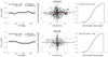 |
Fig. C.1. Diagnostic diagrams of the rotation signature detected in the clusters when considering all their galaxy members. See Fig. 9. |
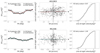 |
Fig. C.2. Diagnostic diagrams of the rotation signature detected in the clusters within 5′ from the center. See Fig. 9. |
Appendix D: Jeans equations with Navarro-Frenk-White density
Fig. D.1 shows the result for the line of sight obtained from the Jeans equation when adopting the NFW profile obtained in Subsect. 6.1.
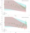 |
Fig. D.1. Line-of-sight velocity dispersion profile of the galactic component obtained from the Jeans equation for AS1063 and M1206 when using an NFW profile for the galaxy number density. See Fig. 13. |
All Tables
Summary of the mean velocities ⟨v⟩sec and velocity dispersion σlos,sec inside each sector.
Cluster parameters derived for the total mass distribution described by a spherical NFW model reconstructed from combined strong-lensing, weak-lensing shear and magnification measurements.
All Figures
|
Fig. 1. View of the cluster members of Abell S1063 (left) and MACS J1206.2−0847 (right). The gray scale background image on the left (right) is the WFI (SUBARU) observation in the Rc band spanning an area of ≈25 × 25 arcmin2. The member galaxies are plotted as colored dots. The colors correspond to the stellar mass values of each galaxy as reported in the color bar. The three concentric yellow circles represent the distances of 1.5, 3, and 4.5 Mpc (1, 3, and 5 Mpc) from the cluster center identified with the BCG. The green rectangle represents the ≈1 × 2 arcmin2 (≈1 × 2.63 arcmin2) area covered by the MUSE spectroscopic follow-up on the inner regions of the cluster. |
| In the text | |
|
Fig. 2. Line-of-sight velocity distribution for the member galaxies of the two clusters. The vertical dashed lines represent the corresponding velocity dispersion σlos. The binning procedure consisted of dividing the range of observed line-of-sight velocities in bins of 200 km s−1. |
| In the text | |
|
Fig. 3. Stellar mass distribution for the two clusters divided into bins of 0.15 dex. Because the individual galaxies also contain DM halos and gas, the total mass distribution would be shifted to the right of the diagram and would possibly have a different shape. |
| In the text | |
|
Fig. 4. Projected number density profile of the galactic component as a function of the radial distance from the cluster center. For each cluster, the circularized radius R was measured in terms of the half-mass radius defined on the basis of its stellar mass distribution. The bins were obtained by dividing the range of observed R/Rhm of each cluster into 20 subintervals. The error bars are 1σ. As briefly described in the text, the profiles are affected by the sample incompleteness in a nontrivial way. |
| In the text | |
|
Fig. 5. Line-of-sight velocity dispersion profile of the galactic component as a function of the radial distance from the cluster center normalized to the global velocity dispersion σlos of each cluster. As in Fig. 4, for each cluster, the circularized radius R was measured in terms of the cluster stellar half-mass radius, and the bins were defined according to the same procedure. The vertical bars represent the errors evaluated as |
| In the text | |
|
Fig. 6. Sample of member galaxies divided into sectors along the major (blue line) and minor (red line) axes for M1206 following the steps introduced in Sect. 4. The dashed yellow circle represents the half-mass radius Rhm. The sectors are identified as sector A in blue, sector B in orange, sector C in green, and sector D in red. If rotation were responsible for the observed flattening, gradients in the line-of-sight galaxy velocity distribution would be expected along the major axes and not along the minor axes. |
| In the text | |
|
Fig. 7. Distribution of the line-of-sight velocities of member galaxies of M1206 contained in the sectors shown in Fig. 6. Upper histogram: stacked distribution of velocities in the four sectors compared to the total velocity distribution of Fig. 2. Lower histograms: velocity distributions of the galaxies in each sector. The sectors are identified as sector A in blue, sector B in orange, sector C in green, and sector D in red. |
| In the text | |
|
Fig. 8. Position-velocity diagrams of the member galaxies within a distance D < (1/2)Rhm from the major (left) and minor (right) axes of AS1063 (cyan) and M1206 (green). These plots do not show any clear rotation signature (which would offset the points in the diagrams toward two diagonally opposite quadrants). |
| In the text | |
|
Fig. 9. Diagnostic diagrams of the rotation signature detected in the core of the two clusters within 0.5′ from the center. This corresponds to the areas covered by the MUSE pointings. The left panels show the difference between the mean velocities ΔVmean on each side of a line passing through the center with the given angle (PA) divided by the velocity dispersion |
| In the text | |
|
Fig. 10. Evidence of mass segregation. The galaxies were divided into bins according to their stellar mass. This plot shows the variation of Rhm(M⋆), which is the half-mass radius of the cluster members inside the nth bin normalized to the global half-mass radius, with galactic mass. The errors were evaluated as |
| In the text | |
|
Fig. 11. Absence of energy equipartition. The galaxies are divided in bins according to their stellar mass. This plot shows the variation of σlos(M⋆), which is the velocity dispersion of the cluster members inside the nth bin normalized to the global velocity dispersion, with galactic mass. The errors were evaluated as |
| In the text | |
|
Fig. 12. Observed surface number density of AS1063 (in green) fitted with the projected Jaffe, dPIE, and NFW profiles (in red). Top row: profiles resulting from the best-fit process. Bottom row: fractional deviations between the analytical model and the photometric data. The labels provide the reduced χ2 values. |
| In the text | |
|
Fig. 13. Line-of-sight velocity dispersion profile of the galactic component obtained from the Jeans equation for AS1063 and M1206. The plots show the data points (in green) derived from the spectroscopic data (see Fig. 5) superimposed on the velocity profiles derived from the Jeans equation for two choices of β(r): the constant isotropic β = 0 profile (in cyan) and the Osipkov–Merritt anisotropy profile (in red). The confidence regions were found by allowing the total mass M(r) to vary within the uncertainties of the values of its parameters reported in Table 4. The confidence levels were underestimated for R > 3 Mpc because, in this region, the total mass M(r) is extrapolated and not directly constrained by the observations. |
| In the text | |
|
Fig. 14. Line-of-sight velocity dispersion profile of the galactic component derived from the f(ν) distribution function with fitted parameters for AS1063 and M1206 (see Table 6). The plot shows the data points (in black) derived from spectroscopic data (see Fig. 5) superimposed on the velocity profiles derived from the moments of the distribution function for five choices of the value of the parameter d (see Fig. 16 for the associated anisotropy profile). Both clusters are well described by the velocity dispersion curves associated with a value of d ≈ 10 − 50. |
| In the text | |
|
Fig. 15. Projected number density profile of the galactic component derived from the f(ν) distribution function with fitted parameters for AS1063 and M1206 (see Table 6). The plot shows the data points (in black) derived from photometric data (see Fig. 4) superimposed on the projected number density profile derived from the moments of the distribution function for five choices of the value of the parameter d (see Fig. 16 for the associated anisotropy profile). The value of the parameter A was obtained after a best-fit against the observed profile performed within 2Rhm. Both clusters are well described by the curves associated with a value of d ≈ 10 − 50, confirming the results of Fig. 14. |
| In the text | |
|
Fig. 16. Anisotropy parameter radial profile. The colored solid lines show the anisotropy profile as a function of the free parameter d. The distribution of the stellar orbits associated with the adopted distribution function is characterized by isotropy in the central region and radially biased anisotropy in the outer parts, which becomes more prominent as the value of d increases. The dashed, dashed-dotted, and dotted gray curves represent, respectively, the isotropic, radial, and Osipkov–Merritt anisotropy profiles of Table 5. |
| In the text | |
|
Fig. C.1. Diagnostic diagrams of the rotation signature detected in the clusters when considering all their galaxy members. See Fig. 9. |
| In the text | |
|
Fig. C.2. Diagnostic diagrams of the rotation signature detected in the clusters within 5′ from the center. See Fig. 9. |
| In the text | |
|
Fig. D.1. Line-of-sight velocity dispersion profile of the galactic component obtained from the Jeans equation for AS1063 and M1206 when using an NFW profile for the galaxy number density. See Fig. 13. |
| In the text | |
Current usage metrics show cumulative count of Article Views (full-text article views including HTML views, PDF and ePub downloads, according to the available data) and Abstracts Views on Vision4Press platform.
Data correspond to usage on the plateform after 2015. The current usage metrics is available 48-96 hours after online publication and is updated daily on week days.
Initial download of the metrics may take a while.