| Issue |
A&A
Volume 676, August 2023
|
|
|---|---|---|
| Article Number | A85 | |
| Number of page(s) | 30 | |
| Section | Catalogs and data | |
| DOI | https://doi.org/10.1051/0004-6361/202346108 | |
| Published online | 11 August 2023 | |
The ESO UVES/FEROS Large Programs of TESS OB pulsators
I. Global stellar parameters from high-resolution spectroscopy★
1
Institute of Astronomy, KU Leuven,
Celestijnenlaan 200D,
3001
Leuven, Belgium
e-mail: This email address is being protected from spambots. You need JavaScript enabled to view it.
2
Max Planck Institute for Astronomy,
Königstuhl 17,
69117
Heidelberg, Germany
3
Royal Observatory of Belgium,
Ringlaan 3,
1180
Brussels, Belgium
4
Department of Astrophysics, IMAPP, Radboud University Nijmegen,
PO Box 9010,
6500 GL
Nijmegen, The Netherlands
Received:
8
February
2023
Accepted:
16
May
2023
Abstract
Context. Modern stellar structure and evolution theory suffers from a lack of observational calibration for the interior physics of intermediate- and high-mass stars. This leads to discrepancies between theoretical predictions and observed phenomena that are mostly related to angular momentum and element transport. Analyses of large samples of massive stars connecting state-of-the-art spectroscopy to asteroseismology may provide clues as to how to improve our understanding of their interior structure.
Aims. We aim to deliver a sample of O- and B-type stars at metallicity regimes of the Milky Way and the Large Magellanic Cloud (LMC) galaxies with accurate atmospheric parameters from high-resolution spectroscopy, along with a detailed investigation of line-profile broadening, both for the benefit of future asteroseismic studies.
Methods. After describing the general aims of our two Large Programs, we develop a dedicated methodology to fit spectral lines and deduce accurate global stellar parameters from high-resolution multi-epoch UVES and FEROS spectroscopy. We use the best available atmosphere models for three regimes covered by our global sample, given its breadth in terms of mass, effective temperature, and evolutionary stage.
Results. Aside from accurate atmospheric parameters and locations in the Hertzsprung-Russell diagram, we deliver detailed analyses of macroturbulent line broadening, including estimations of the radial and tangential components. We find that these two components are difficult to disentangle from spectra with signal-to-noise ratios of below 250.
Conclusions. Future asteroseismic modelling of the deep interior physics of the most promising stars in our sample will provide much needed information regarding OB stars, including those of low metallicity in the LMC.
Key words: stars: fundamental parameters / stars: massive / stars: early-type / stars: rotation / asteroseismology / stars: oscillations
Based on observations collected at the European Southern Observatory, Chile under programs 1104.D-0230 and 0104.A-9001.
© The Authors 2023
 Open Access article, published by EDP Sciences, under the terms of the Creative Commons Attribution License (https://creativecommons.org/licenses/by/4.0), which permits unrestricted use, distribution, and reproduction in any medium, provided the original work is properly cited.
This article is published in open access under the Subscribe to Open model. This email address is being protected from spambots. You need JavaScript enabled to view it. to support open access publication.
1 Introduction
The field of stellar astrophysics was revolutionised with the advent of space missions such as CoRoT (Auvergne et al. 2009), Kepler/K2 (Borucki et al. 2010), and TESS (Ricker et al. 2015). This revolution became possible thanks to the high-duty-cycle, nearly uninterrupted, and unprecedentedly long (from about 1 month in a single TESS sector to 4 years for the entire Kepler nominal mission duration) photometric time series at the sub-millimagnitude(sub-mmg) level of precision that these missions delivered. Such high-precision data are currently available for tens of thousands of stars. These ensembles provide stringent tests for theories of stellar structure, evolution, atmospheres, tidal interactions, and so on. In particular, numerous recent studies point to both severe and less critical deficiencies in the above-mentioned theories, notably in regard to angular momentum transport and chemical mixing. Some of the deficiencies remain unresolved, whereas others are currently being tackled in detail thanks to theoretical improvements (e.g. Mosser et al. 2012; Beck et al. 2012; Fuller & Lai 2012; Cantiello et al. 2014; Deheuvels et al. 2016; Fuller 2017; Fuller et al. 2017; Hekker & Christensen-Dalsgaard 2017; Aerts et al. 2019; Bowman 2020; Deheuvels et al. 2020; Aerts 2021; Southworth 2021).
The study of binary stars has received a major boost in recent years. This is in part associated with the superior quality of the space-based photometry when compared to its ground-based counterpart, but is also due to synergies enabled by various types of intrinsic variability often observed in one or both of the binary components. Indeed, solid observational detections of tidally induced pulsations were reported in the HD 174884 system observed by CoRoT (Maceroni et al. 2009), followed by the discovery of high-amplitude tidally induced oscillations in the Kepler object of interest KOI-54 (Welsh et al. 2011). The observed properties of KOI-54 were subsequently modelled by Fuller & Lai (2012). Numerous binary systems with stellar pulsations that are either induced or perturbed by tides have also been found and modelled (e.g. Bowman et al. 2019b; Guo et al. 2019; Handler et al. 2020; Kurtz et al. 2020; Fuller et al. 2020; Fuller 2021; Rappaport et al. 2021; Lee 2021; Van Reeth et al. 2022; Jayaraman et al. 2022). There have been notable applications of space-based photometry for the class of highly eccentric systems dubbed ‘heart-beat stars’ (e.g. Thompson et al. 2012; Hambleton et al. 2013, Hambleton et al. 2016; Beck et al. 2012; Guo et al. 2020; Cheng et al. 2020; Kołaczek-Szymanski et al. 2021). Furthermore, a sample of low- and intermediate-mass binaries observed by Kepler has enabled empirical tests of state-of-the-art tidal evolution theory (Zahn 2013) with respect to its predictions for the circularisation of binary orbits (Van Eylen et al. 2016). Ultimately, (eclipsing) binary stars allow us to constrain the amount of core-boundary mixing and the convective core masses in intermediate- and high-mass stars (e.g. Claret & Torres 2018, 2019; Tkachenko et al. 2020; Johnston 2021, and references therein) thanks to the unique property of eclipsing, with spectroscopic double-lined binaries delivering masses and radii with precision and accuracy reaching a level of 1%, and in some cases even better (e.g. Maxted & Hutcheon 2018; Maxted et al. 2020; Mahy et al. 2020a,b; Serenelli et al. 2021; Pavlovski et al. 2022).
Yet another field in stellar astrophysics that has seen enormous advances with the launch and operation of space-based missions is asteroseismology. This field exploits the fact that, as stars evolve and cross different regions in the HertzsprungRussell (HR) diagram, they become unstable to pulsations. Two principle types of stellar pulsation are distinguished by their dominant restoring force: pressure (p) modes, which are acoustic waves dominantly restored by pressure gradients, and gravity (g) modes restored by buoyancy. While p modes are typically confined to the envelope of stars, g modes have their largest amplitudes in the near-core regions and are therefore most sensitive to the physical conditions in the deep stellar interior. One of the outstanding observational findings of space-based missions is that the vast majority of stars are intrinsically variable, and that pulsating stars are found everywhere across the HR diagram (Aerts 2021; Kurtz 2022).
Asteroseismology, which probes the near-core region in intermediate- to high-mass stars (spectral types early-F to late-O), had to await space-based observations owing to the long periods of their g modes (of the order of 1 day). Theoretically predicted informative series of (quasi-)uniformly spaced g-mode periods, dubbed period spacing patterns (Miglio et al. 2008; Bouabid et al. 2013), were only recently detected from space-based photometric observations of B- and F-type stars (e.g. Van Reeth et al. 2015a,b; Pápics et al. 2017; Szewczuk et al. 2021). Detailed asteroseismic modelling of the period spacing patterns enables probes of the level and functional form of convective core boundary and envelope mixing (e.g. Moravveji et al. 2015, 2016; Szewczuk & Daszyńska-Daszkiewicz 2018; 2019, 2021; Mombarg et al. 2019, 2021; Pedersen et al. 2018, 2021; Pedersen 2022; Bowman & Michielsen 2021; Szewczuk et al. 2022), internal rotation (e.g. Triana et al. 2015; Van Reeth et al. 2016, 2018; Ouazzani et al. 2017, 2020; Li et al. 2020), the physics of radiative levitation (Deal et al. 2016, 2017; 2020, 2022), and the impact of magnetism (Buysschaert et al. 2018; Lecoanet et al. 2022) in these stars. In particular, these and other studies lead to the conclusion that standard stellar structure and evolution models of intermediate- and high-mass stars incorrectly predict their convective core masses (e.g. Johnston 2021, and references therein) and lack mechanism(s) of efficient angular momentum transport beginning in their longest and most stable main sequence stage of evolution (e.g. Aerts et al. 2017a, 2019; Aerts 2021, and references therein). These conclusions for the main sequence are in agreement with both observational and numerical studies of intermediate-mass stars in post-main sequence stages (e.g. Mosser et al. 2012; Beck et al. 2012; Cantiello et al. 2014; Hermes et al. 2017; Aerts et al. 2019).
Typically, space-based photometry in tandem with ground-based spectroscopy reveal pulsators in regions in the HR diagram where they were not expected. On the other hand, a lack of pulsation signatures is sometimes found in stars that are expected to pulsate according to their location in the HR diagram. For example, recent studies of A- and F-type stars based on Kepler and Gaia photometric data reveal a considerable fraction of pulsators outside of their respective theoretical instability regions (e.g. Uytterhoeven et al. 2011; Bowman & Kurtz 2018; Murphy et al. 2019; Gaia Collaboration 2023). On the other hand, Balona (2014) and Balona et al. (2015) report that at least 50% of A-type stars do not pulsate while being located within the borders of the theoretical instability strips. Furthermore, Balona & Ozuyar (2020) find a group of B-type stars pulsating with high frequency while being too cool to be explained as rapidly rotating β Cep-type p-mode pulsators, whose effective temperature is substantially affected by gravity darkening. Such stars are found in both ground-based and space-based high-cadence photometry and are rather interpreted as slowly pulsating B (SPB) stars whose observed (prograde) g-mode frequencies are shifted to high frequencies - sometimes above ~3 d−1 – by the influence of Coriolis acceleration on the modes and by the Doppler effect (Aerts & Kolenberg 2005; Saesen et al. 2010, 2013; Mowlavi et al. 2013, 2016; Moździerski et al. 2014, 2019; Sharma et al. 2022; Gebruers et al. 2022; Gaia Collaboration 2023). This interpretation is in agreement with the theoretical computations by Bouabid et al. (2013) and Salmon et al. (2014).
Stars of spectral type O and B were under-represented in the nominal Kepler field as its selection was dictated by the mission’s core science goal of detecting exoplanets orbiting solar-type stars. Moreover, models of these intermediate- to high-mass stars are the most uncertain among those in stellar evolution computations (e.g. Martins & Palacios 2013). This current state of affairs motivates us to look closely at photometric data delivered by the all-sky TESS mission, as its observational strategy does not bias against O and B stars and allows us to target these objects both in the Milky Way and Large Magellanic Cloud (LMC) galaxies. The LMC is a challenging laboratory for testing the theory regarding heat-driven stellar pulsations, as this latter depends strongly on metallicity. The lower metallicity of the LMC and its implied low number of predicted pulsators is therefore of particular interest (cf., Salmon et al. 2014). Preliminary investigations of TESS data for massive stars in the LMC indeed indicate few heat-driven pulsators (Bowman et al. 2019a).
The current paper is the first in a series aiming at a full application of asteroseismology to O and B stars with a combined approach using space photometry and astrometry together with high-resolution spectroscopy. As is necessarily the case in asteroseismology for massive stars, given the nature of the oscillation characteristics of those stars, this is a long-term project and the overall study involves several (PhD) subprojects. Here, we first present the aims of the overall project and subsequently focus on the derivation of the global spectroscopic parameters of the target stars, which were selected from Cycle 1 TESS space-based photometry. In Sect. 2, we present our concrete scientific motivations, the role of TESS space-based photometry, the aster-oseismic quantities we are seeking to obtain, the role of the ESO high-resolution ground-based spectroscopy in our Large Programs, and our sample selection. Our spectroscopic observations and custom data processing are described in Sect. 3, while spectroscopic classification, inference of atmospheric parameters, and investigation of line-broadening mechanisms in the spectra of the sample stars are detailed in Sect. 4.
We provide a detailed discussion of the obtained results, keeping in mind the photometric classification of stars from Cycle 1 TESS photometry, and conclude the paper in Sect. 6. Subsequent papers will tackle abundance determinations, frequency analyses from the full Cycle 1 to Cycle 4 TESS photometric light curves, and stellar modelling for all O and B pulsators with sufficient identified modes based on all observational input, including all the Gaia data that will be available at that stage of our project.
2 Two ESO Large Programs with the FEROS and UVES spectrographs
2.1 Overall project goals
The ultimate goal of our two ESO Large Programs (UVES: 1104.D-0230; FEROS: 0104.A-9001) is to remedy the current lack of high-precision observational calibration for the theoretical description of stellar interiors in stellar structure and evolution models of intermediate- to high-mass stars. Our concrete goals can only be achieved by exploiting complementary (ESO) high-resolution spectroscopy along with TESS space-based photometry and Gaia astrometry for a wide range of stellar masses covered by OB(AF)-type stars.
With our two Large Programs, we aim to (i) resolve the current two-orders-of-magnitude discrepancy between theory and observations of angular momentum transport; (ii) deliver astero-seismically calibrated mixing profiles for stellar interiors, which currently do not exist in a quantitative sense for high-mass stars and are scarce for intermediate-mass stars; (iii) challenge state-of-the-art models of stellar structure and pulsations by searching for coherent g-mode pulsators in the low-metallicity regime of the LMC; and (iv) investigate possible connections between coherently and/or stochastically excited gravity waves and turbulent velocity fields in the atmospheres of OB stars. Furthermore, our program is designed in such a way as to enable observational check for binarity, which also allows us to deliver an unprecedented legacy for future studies of pulsators in (close) binaries. Tidal asteroseismology is capable of quantifying the effect of tides by investigating the internal rotation and mixing in close binaries and comparing these to their counterparts in the single-star case (e.g. Guo 2021; Lampens 2021, for reviews).
2.2 Asteroseismology of massive stars: The role of TESS
Unlike ‘classical’ observational methods (e.g., snapshot spectroscopy and multi-colour photometry), which largely concern surface properties of stars, asteroseismology offers insight into the internal physics of stars through the interpretation of detected and identified stellar oscillations. It is therefore an optimal tool with which to evaluate and calibrate models of stellar interiors, provided that we can detect and identify sufficient modes in terms of their l, m, and n numbers (Aerts et al. 2010a).
In terms of angular momentum transport in intermediate-mass dwarfs, the asteroseismic ensemble studies by Van Reeth et al. (2016, 2018), Aerts et al. (2017b), and Ouazzani et al. (2019) demonstrate that stars born with a convective core tend to show almost rigid rotation in their radiative envelopes independent of their near-core rotation rate and evolutionary stage. This implies that strong coupling between the convective core and radiative envelope occurs on the main sequence. This conclusion is based on studies of stars with masses of between 1.3 M⊙ and 9 M⊙, with the mass distribution being largely skewed towards late-B and F-type stars (M ≲ 3.0 M⊙). It is only for this mass regime that the later evolutionary stages have been mapped in great detail (e.g. Aerts et al. 2019, for a review). The goal of our ESO UVES+FEROS Large Programs is to expand the parameter space towards the higher stellar mass regime (M ≳ 3.0 M⊙) by focusing on stars of spectral types O and B on the main sequence, and on those in the hydrogen-shell and core-helium burning phases covered by blue supergiants. These phases constitute ~90% of the total lifetime of massive stars, excluding the remaining short period prior to the remnant formation when considerable mass loss occurs due to a radiation- or dust-driven wind. During this final phase, the unambiguous detection of modes is challenging due to the strong wind.
Previously, analyses of the CoRoT and Kepler/K2 photometric data revealed the presence of non-radial oscillation modes in core-hydrogen burning stars with masses of between 3 and ~ 25 M⊙ (e.g. Neiner et al. 2009; Huat et al. 2009; Diago et al. 2009; Gutiérrez-Soto et al. 2009; Degroote et al. 2010a; Briquet et al. 2011; Mahy et al. 2011; Thoul et al. 2013; Buysschaert et al. 2015; Pápics et al. 2017; Szewczuk et al. 2021; Pedersen et al. 2021) and in blue supergiants (Aerts et al. 2010b, 2017a, 2018; Simón-Díaz et al. 2018). Forward asteroseismic modelling is only available for about 30 of them, with quite different levels of depth (Aerts et al. 2011; Briquet et al. 2011; Neiner et al. 2012; Moravveji et al. 2015, 2016; Michielsen et al. 2021; Pedersen et al. 2021). The majority of the other intermediate-to-high-mass pulsators lack proper mode identification, particularly for those with short light curves (less than half a year). Prior to space aster-oseismology, long-term ground-based campaigns had already led to such modelling for a few bright β Cep stars, albeit based on only a few identified modes (Aerts et al. 2003; Handler et al. 2006, 2009; Dziembowski & Pamyatnykh 2008; Briquet et al. 2012).
CoRoT data gave rise to the detection of stochastic high-frequency oscillations in a few OB-type stars (Belkacem et al. 2009; Degroote et al. 2010b), driven by either turbulent envelope convection (Belkacem et al. 2010) or non-linear resonant mode coupling (Degroote et al. 2009). Moreover, Blomme et al. (2011) found stochastic low-frequency (SLF) variability in the CoRoT data of several rapidly rotating O-type stars. SLF variability was later found to be present – often in addition to coherent oscillation modes – for the vast majority of O and B stars observed with CoRoT or K2 (Bowman et al. 2019c).
A similar discovery was made for a sample of some 50 LMC O- and B-type stars observed with TESS (Bowman et al. 2019a). The lack of dependence of the properties of SLF variability on the metallicity of the star and its apparent scaling with the stellar (convective core) luminosity led to the interpretation that internal gravity waves (IGWs) excited stochastically at the core boundary are the cause of the observed photospheric variability (see e.g. Rogers et al. 2013; Edelmann et al. 2019; Ratnasingam et al. 2020; Horst et al. 2020), although alternative interpretations have also been suggested (Lecoanet et al. 2019). In any case, SLF variability is ubiquitious in OB stars and is related to their mass and age (Bowman et al. 2020).
In conclusion, too few O- and B-type pulsators have been modelled in sufficient asteroseismic depth to improve the physics of stellar interiors for stars with masses above ~ 5 M⊙ (Bowman 2020). This is why we turn our attention to the TESS mission, which offers hundreds of potential massive candidate pulsators with high-cadence photometry covering at least 6 months of uninterrupted light curves, following our approved TESS guest observer programs covering cycles 1 to 5 of the extended mission (PI Bowman1).
2.3 The quest for mixing and rotation profiles
Because coherent g-modes and stochastically excited IGWs are both confined to the low-frequency regime (typically below some 3 d−1 or ~35 μHz), while asteroseismic analyses require individual pulsation modes to be resolved, our goals can only be achieved by exploiting TESS light curves of longer duration than the CoRoT light curves. Therefore, we focus on OB stars in the Southern Continuous Viewing Zone (CVZ-S) of TESS and its vicinity, which are the regions of the sky for which there are high-duty-cycle photometric data of between approximately 200 d and 1 yr in duration, which is long enough to enable both p- and g-mode asteroseismology. We take an observationally driven approach with the goal being to estimate the following three quantities for a representative sample of single intermediate- and high-mass stars from their asteroseismic analysis: (i) Ω(r, t) – the interior rotation frequency and its evolution in time, (ii) Dov(r, t) – the convective core overshooting profile and its evolution in time, and (iii) Dmix(r, t) – the chemical mixing profile in the radiative envelope and its evolution in time. Here, t is the age of the star and r ∈ [0, R(t)] is the depth inside the star from the centre, r = 0, to the surface at r = R(t). The quantity Dmix(r, t) captures the cumulative effect of all active mixing phenomena in the radiatively stratified envelope from the star’s birth until t.
With the addition of the four minimum free parameters that are required to compute evolutionary models, namely the stellar mass M, the initial hydrogen and metal mass fractions (X, Z), and the age t, asteroseismology is found to be at least a seven-dimensional (7D) problem, even in the simplest case where the three above-mentioned internal profiles only have one free parameter that does not change in time. However, as shown by Van Reeth et al. (2016), this 7D estimation problem can be broken down into a multi-step approach. In particular, interpretation of the period spacing patterns of g modes (cf. Sect. 1) allows us to estimate the near-core rotation frequency of the star, Ωcore (Van Reeth et al. 2016; Ouazzani et al. 2017; Li et al. 2020). Furthermore, the inclusion of envelope mixing Dmix(r) appreciably affects high-order g modes and determines the surface abundances of CNO-produced chemical elements. In addition, g modes are capable of differentiating between different Dov(r) profiles for main-sequence stars (Pedersen et al. 2018, 2021; Pedersen 2022; Michielsen et al. 2019, 2021). This way, combined asteroseismology and surface abundance information can be used to constrain the amount and functional form of mixing in both the near-core region and radiative envelope of intermediate-to high-mass stars. Aerts et al. (2018) provided methodology for a forward asteroseismic modelling that encapsulates all of the above-described analysis steps, and relies on state-of-the-art statistical principles to account for theoretical model-prediction uncertainties as well as strong correlations among the numerous free parameters being estimated.
2.4 The role of ESO high-resolution spectroscopy
High-quality spectroscopic observations are essential to addressing the above science questions and to meeting our goals. We therefore applied for high-resolution (R ≳ 40000), high-signal-to-noise-ratio (S/N ~ 100) two-epoch spectroscopy for a sample of TESS O- and B-type variable stars in the Milky Way and LMC galaxies. These data were obtained with the Ultraviolet and Visual Échelle Spectrograph (UVES; Dekker et al. 2000) and the Fiber-fed Extended Range Optical Spectrograph (FEROS; Kaufer et al. 1999) instruments attached to the UT2@VLT and MPG/ESO 2.2 m telescopes, respectively.
UVES is a cross-dispersed échelle spectrograph that covers the entire optical range with its two arms (300–500 nm and 420–1100 nm in the blue and red arms, respectively) and offers a variety of spectral resolving power possibilities (up to 80 000 and 110 000 in the blue and red arm, respectively) regulated by the slit width of the instrument. We opted for the UVES2 DIC-2 blue arm standard setting (CD2, 437+760 nm) as it covers a number of Balmer (including Hα) and helium lines – the main diagnostic lines for the determination of fundamental atmospheric parameters – as well as important diagnostic lines of metals for the determination of v sin i, micro- and macro-turbulent velocities, and surface abundances of OB stars. Because massive stars are typically moderate to fast rotators, we chose a slit width of 1 arc-second, corresponding to a resolving power of R ~ 40 000, which is sufficient to properly resolve individual lines in the spectra of these stars.
FEROS3 is a fibre-fed échelle spectrograph covering the wavelength range from 350 nm to 920 nm. It operates at a resolving power of R ~ 48 000. This combination of a wide wavelength range and high spectral resolution makes the instrument ideal for providing the stellar astrophysics community with high-quality spectroscopic observations of relatively bright stars, including intermediate- to high-mass stars of spectral types O and B.
2.5 Sample selection
Our sample selection is largely based on the studies of massive stars by Bowman et al. (2019a) and Pedersen et al. (2019) with respect to their photometric variability as detected in the first sector(s) of TESS data. We complement the samples of these latter authors with a global search for stars of spectral types O and B in the Southern CVZ of TESS using the infrastructure and functionality of the Simbad astronomical database4 (Wenger et al. 2000). We cross-matched this obtained list of OB targets with the catalogues of Bowman et al. (2019a,b, 2020), and Pedersen et al. (2019), and the targets that did not have a match were kept in the sample for further consideration. For these extra targets, we performed custom extraction of their light curves from the TESS Full Frame Images (FFIs) and performed their visual photometric variability classification based on the dominant signal detected in the TESS data. All eclipsing binaries have been excluded, making our sample biased against this type of object — TESS (pulsating) eclipsing binaries constitute a separate (PhD) study (cf., IJspeert et al. 2021). We thereby reduced our sample to slightly over 350 targets, which were prioritised according to their potential for future asteroseismic modelling. All stars were subjected to a check for existing spectroscopic data of required quality (R ≳ 40 000 and S/N ~ 100) and cadence (minimum two epochs) in public (including ESO) archives.
We were left with a total of 272 stars that we ultimately targeted with the UVES and FEROS instruments. The sample was divided in two parts according to the V-band magnitudes of the targets. Fainter stars with Vmag > 10 were observed with the UVES instrument, while brighter objects with Vmag ≤ 10 were targeted with the FEROS instrument. This strategy allowed us to achieve maximal observing efficiency. In particular, this implied that none of the UVES science exposures were dominated by the instrument’s system overhead.
The choice to take two-epoch spectroscopic observations was driven by the need to (i) uncover potential binaries in our sample, and to (ii) detect possible variations in spectral lines (He, Si, Mg, etc.) due to large macroturbulent velocity fields. High values of macroturbulence were previously reported for many high-mass stars (e.g. Simón-Díaz & Herrero 2014; Simón-Díaz et al. 2017). Moreover, a link between the physics underlying this phenomenon and non-radial gravity modes and/or IGWs has been suggested (Aerts & Rogers 2015; Bowman et al. 2020). Uncovering binaries is crucial in order to distinguish between intrinsic variability and perceived variability due to strong tidal interactions between stars in a (close) binary system. The two spectroscopic observations per object have been separated by at least 2–3 weeks to ensure detection capability for both short-and intermediate-period binaries where tidal forces are expected to be strongest.
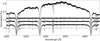 |
Fig. 1 UVES spectrum of Galactic main sequence star HD 41297. Panel a shows the order-merged non-normalised spectrum extracted with the ESO data reduction pipeline. Panels b, c, and d demonstrate the spectra normalised by fitting a low-degree polynomial to the individual échelle orders, fitting a 2D smoothing spline to all 30 échelle orders in the UVES blue arm, and iterative fitting of synthetic spectra, respectively. The best-fit synthetic spectrum obtained for this star is shown in panel e for comparison. See text for details. |
2.6 Further content and goals of this paper
As of now, we focus on the global spectroscopic analysis of part of our overall stellar sample of 272 OB stars in the Galaxy and LMC. In particular, we carry out an analysis of the entire UVES sample of 105 stars, composed of mostly blue supergiants in the LMC and a few dwarfs in the Milky Way. We extend this sub-sample with 43 LMC blue supergiant stars observed with the FEROS instrument, bringing the total of treated stars in this paper to 148. The remaining 124 Galactic objects (98 single stars and 26 spectroscopic binaries) in the FEROS sample are analysed and presented in the accompanying paper by Gebruers et al. (2022).
Our goal for the 148 OB stars (of which 24 are duplicates, i.e. stars observed with both instruments) treated here is twofold: (i) We perform a check for binarity and derive stellar atmospheric parameters such as the effective temperature Teff, surface gravity log g, and projected rotational velocity ν sin i; and (ii) should the data quality allow for it, we investigate the effect of macro-turbulent broadening on spectral lines across the sample and its possible connection with stellar oscillations. In the final section, we reconsider the TESS variability classification of the stars according to their spectroscopic parameters.
3 Custom spectroscopic data reduction
The power of asteroseismology for probing the effects of mixing in the radiative envelopes and atomic diffusion in intermediate-to high-mass stars is greatly increased when high-precision inference of atmospheric chemical composition is available for these stars (e.g. Mombarg et al. 2022). The high precision required for the determination of atmospheric parameters and chemical composition of stars can only be achieved when the raw spectra are extracted and normalised to the local continuum in an optimal way. As mentioned in Sect. 2, a subsample of 124 Galactic objects from our program targeted with the FEROS instrument are analysed in the accompanying paper by Gebruers et al. (2022), where a modified version of the CERES data reduction pipeline5 (Brahm et al. 2017) was used to achieve the required precision in the processed spectra.
In this work, we employ the ESOREFLEX data reduction pipeline6 (Freudling et al. 2013) to process the data obtained with the UVES instrument. The data reduction steps include bias subtraction, flat fielding, wavelength calibration, order merging, and removal of cosmic hits. Figures 1a and 2a show the extracted, wavelength-calibrated, order-merged UVES spectra of an example main-sequence star, HD 41297, and an example blue supergiant, HD 270123, respectively. Both spectra contain a prominent wave-like pattern reminiscent of the individual échelle orders, and this pattern is detected in the reduced spectra of most of our targets. The pattern cannot be properly accounted for during the normalisation process and strongly affects the end results, especially in the wavelength regions of broad hydrogen lines in the spectra of main sequence stars.
Given that the inferior quality of the spectrum extraction and normalisation is in direct conflict with our needs for future high-precision asteroseismic modelling, we opt to develop a custom reduction pipeline instead. We start with an intermediate product of the ESO pipeline in the form of the blaze-corrected, non-merged échelle orders. These non-merged spectra are subjected to normalisation to the local continuum where we consider the following two approaches: (i) an ‘order-by-order’ method where each individual échelle order is normalised independently by fitting a low-degree polynomial to it (dubbed ‘method 1’), and (ii) a ‘2D method’ where all 30 échelle orders in the blue arm are considered as an ensemble and approximated by a 2D surface of cubic smoothing splines (dubbed ‘method 2’). The individual normalised orders are ultimately merged together with the flux being represented by the weighted mean in the overlapping regions of the consecutive orders. The weights are assumed to be increasing with the distance from the edge of the order such that the order edges – characterised by high levels of noise – provide a negligible contribution to the mean flux value.
We find that these two new methods give comparable results. Typical examples of the normalised spectra are shown in Figs. 1b,c and 2b,c for a Galactic main sequence star with broad hydrogen lines and a blue supergiant in the LMC, respectively. We find that in the case of blue supergiants that do not display broad hydrogen lines spanning the whole échelle order or beyond (cf. Fig. 2c), a simple order-by-order-based method leads to normalised spectra of high quality. In particular, these spectra are free from the pattern reminiscent of the individual échelle orders, which is otherwise present when the normalisation is performed on the order-merged spectra delivered by the ESO data reduction pipeline.
In the case of main sequence stars whose broad hydrogen lines often span the whole échelle order, or even extend beyond a single échelle order, neither of the above-described normalisation methods delivers satisfactory results. We find that the outer wings of hydrogen lines appear to be most affected by the normalisation process (cf. Fig. 1c), which in turn leads to erroneous inference of Teff and log g of the star. In the accompanying paper by Gebruers et al. (2022), a method that assumes simultaneous optimisation of stellar atmospheric parameters and properties of the normalisation function is discussed and employed for the analysis of B- and A-type main sequence stars. Here, we follow a similar approach. The general premise is to use information on the local continuum placement from a grid of synthetic spectra that spans the parameter range of O- and Β-type stars. We employ the Grid Search in Stellar Parameters (GSSP; Tkachenko 2015) software package7 to compute a grid of synthetic spectra in the region of the parameter space corresponding to late B-type stars, while O- and early B-type stars are represented by the OSTAR2002 (Lanz & Hubeny 2003) and BSTAR2006 (Lanz & Hubeny 2007) TLUSTY grids.
The normalisation procedure (dubbed ‘method 3’) consists of the following steps: (i) the blaze-corrected non-merged observed UVES spectrum is taken as input and all individual échelle orders are normalised by dividing with low-degree (n = 3) Chebyshev polynomial functions; (ii) the coefficients of the individual Chebyshev polynomials are optimised by minimising the difference between the normalised échelle order and synthetic spectrum in the wavelength range covered by that order; (iii) all individual normalised échelle orders are ultimately merged together in a weighted scheme similar to the one described above; and (iv) the best-fit synthetic spectrum and normalisation function are obtained by minimising the χ2 merit function across the entire grid of synthetic spectra in the wavelength range between 4000 and 5000 Å. Figure 1d shows the spectrum of an example main sequence star, HD 41297, normalised using the procedure described above. The difference in quality of normalisation with respect to all other methods considered in this work is most noticeable around the Balmer lines, though small-scale improvements in normalisation are also seen throughout the entire wavelength interval.
For completeness, we apply method 3 to the spectrum of blue supergiant stars. As can be seen in the typical example in Fig. 2d, there is no improvement in the quality of normalisation compared to the less complex recipe of the order-by-order normalisation method. On the contrary, the quality gets poorer in wavelength regions associated with the edges of those échelle orders that are rich with rather narrow absorption features. Therefore, in the rest of this work, we adopt the spectrum normalisation method 1 for all blue supergiants in our sample.
In order to validate spectrum normalisation method 3, we pick two main sequence stars, HD 41297 and HD 45527, which were also observed with the FEROS instrument and analysed in Gebruers et al. (2022). In the latter study, the FEROS spectra were processed with the modified version of the CERES data reduction pipeline and subsequently analysed with the ZETA-PAYNE method (Straumit et al. 2022). The ZETA-PAYNE method employs a pre-trained neural network to predict a normalised synthetic spectrum for an arbitrary set of stellar labels such as Teff, log g, v sin i, and [M/H] (and optionally microturbulence ξ). The normalisation function is represented by a series of Chebyshev polynomials and is optimised in the method along with the above-mentioned atmospheric parameters of the star. Application of our method 3 to the UVES spectra of HD 41297 and HD 45527 delivers atmospheric parameters that are consistent within the 1σ confidence interval with those reported in Gebruers et al. (2022).
Finally, we quantify the effect of spectrum normalisation on the inferred atmospheric parameters of three main sequence stars and three blue supergiants. In this exercise, we consider three different approaches for spectrum normalisation: (i) fitting and dividing the blaze-corrected order-merged observed spectrum (cf. Figs 1a and 2a) with a low-degree polynomial (that is the procedure commonly used in the literature); (ii) our method 1; and (iii) our method 3. All three methods deliver atmospheric parameters for the blue supergiants that are consistent within the 1σ confidence interval. However, for the main sequence stars, we find that our method 3 leads to a substantially better representation of the observed spectrum by the best-fit model and delivers Teff and log g that differ by some 1000 K and 0.9 dex, respectively, from the parameters inferred with the other two methods. Therefore, in the rest of this work, we adopt method 3 for the spectrum normalisation of all main sequence stars in our sample according to the initial type classification of each target (see Sect. 4 for details on classification).
4 Analysis of the UVES and FEROS spectroscopy
In order to provide an empirical estimate of the effective temperature and luminosity of the star and to inform the above-described normalisation process, we first perform an initial classification of all the spectra in our sample. The classification is done by means of visual comparison of the selected spectral line intensities and their ratios to the digital spectral classification atlas of Gray8 (Gray & Corbally 2009). We use the pair of Mg II 4481 Å and He I 4471 Å spectral lines as a main diagnostic to assign a spectral type to all stars in the sample. Luminosity classes were decided upon from the strengths of spectral lines of Si, N, O and Fe, depending on the Teff regime: (i) Si IV 4116 Å to He I 4121 Å and N III 4379 Å to He I 4387 Å line strength ratios for late O-type stars; (ii) O II 4070 Å, 4348 Å, 4416 Å, and Si III 4553 Å spectral line strengths for early B-type stars; and (iii) line strength of the Si II 4128/4130 Å doublet for late B-type stars. In this way, we identify 5, 49, and 63 stars of late O-, early-B, and late-B spectral classes, respectively. Moreover, not unexpectedly, we confirm that our sample is dominated with evolved blue supergiants (see Table A.1).
4.1 Identification of line profile variations and binary candidates
Our strategy of multi-epoch spectroscopic observations allows us to check all our targets for a possible binary nature and for particularly strong line profile variations (LPVs) due to intrinsic variability of the star. Both of these phenomena are readily revealed in the analysis of radial velocity (RV) variations that occur due to either global line shifts in the spectra of spectroscopic binaries or line distortions (asymmetries, skewness, etc.) due to variability intrinsic to the star (abundance spots, pulsations, etc.).
We employ the Least-Squares Deconvolution (LSD; Donati et al. 1997) method as implemented in Tkachenko et al. (2013) to compute high-S/N average profiles from the absorption lines for all our targets. These average profiles are subsequently analysed to deduce RV values by fitting them with an asymmetric Gaussian profile of the following form:
 (1)
(1)
Here, r is the asymmetry coefficient, σ controls the width of the profile, and x0 represents the position of the minimum of the profile.
Spectroscopic classification of a star that presumably shows line profile variations due to its intrinsic variability requires a joint interpretation of the inferred RV and coefficient of asymmetry (cf. Aerts et al. 1999; De Cat & Aerts 2002; Telting et al. 2006). We classify a star as a spectroscopic binary (dubbed either SB1 or SB2 in Table A.1 for the case of a single- or a double-lined binary, respectively) when (i) the RV difference between the two epochs is larger than 3σ, or when (ii) a global shift of spectral lines and/or a double-lined nature are confirmed visually. We take a conservative 3σ interval to account for the fact that the obtained uncertainties are purely statistical and result from the least-squares fitting method; they are therefore an underestimation, and any systematic uncertainties are ignored. The same two criteria, that is visual inspection and a relative RV difference of below 3σ, are used to classify a star as ‘LPV’ in Table A.1, where the visual inspection focuses on LPV in the form of (local) spectral line distortions instead of global shifts. Furthermore, stars that show large global asymmetries in their observed line profiles are put into a separate class, dubbed ‘asymm’ in Table A.1. Ultimately, stars that do not show significant RV variability nor appreciable line asymmetries in the two observed epochs are classified as apparently constant (dubbed ‘const’ in Table A.1). Ambiguous classifications are also labelled with a question mark. The results of our classification are summarised in Table A.1 (column designated ‘variability’).
We stress that no distinction is made at this stage between the mechanisms behind the intrinsic variability of the star, be it pulsations, rotational modulation, or any other physical mechanism. This is because of the limited amount of available information (only two spectroscopic epochs) and the simplicity of the employed classification method. Figure 3 shows examples of the observed LSD profiles with the best-fit asymmetric Gaussian profile models overlaid for SK -70 77 (top left), HD 268729 (top right), SOI 404 (bottom left), and HD 268654 (bottom right), which represent typical behaviour for different variability groups. These stars are classified as apparently constant (‘const’), spectroscopic binary candidate (‘SB1’), line profile variable (‘LPV’), and one showing appreciable line asymmetries (‘asymm’), respectively.
In this way, we identify 65 (21), 6 (1), 15 (13), and 22 (15) apparently constant stars, stars with LPV, spectroscopic binary candidates, and stars with appreciable line asymmetries, respectively, in the UVES (FEROS) sample. Of those detections, 0 (0), 3 (1), 12 (11), and 9 (12) are tentative classifications meaning that more observational epochs are required to draw definitive conclusions as to the exact type of spectroscopic variability.
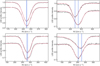 |
Fig. 3 Comparison of the observed LSD profiles with the best-fit asymmetric Gaussian profile models. From top left to bottom right: SK -70 77, HD 268729, SOI 404, and HD 268654 (all were classified as blue supergiants). Blue lines indicate the inferred RVs, while the shaded areas reflect the corresponding 1σ uncertainty intervals. |
4.2 Inference of the projected rotational velocity ν sin i
Measuring the projected rotational velocity ν sin i from the spectrum of an early-type star is not a straightforward task. Lines are typically broadened by several physical mechanisms acting simultaneously in the atmospheres of these stars, ultimately leading to an appreciable overestimation of the ν sin i parameter when other mechanisms are ignored in the analysis. Simón-Díaz & Herrero (2014) and Simón-Díaz et al. (2017) stress that the contribution of a macroturbulent velocity, Θ, to the total broadening of spectral lines in O- and B-type stars can be as large as the contribution associated with ν sin i, and can in many cases even exceed it. Aerts et al. (2014) demonstrate that the macroturbulent and projected rotational velocities cannot be reliably inferred from single snapshot spectroscopic observations of intrinsically variable (spotted and/or pulsating) early-type stars whose spectral lines show pronounced LPV. In particular, the authors stress that ν sin i and Θ vary appreciably and in anti-phase with each other during the pulsation cycle, where Θ can vary by as much as a few tens of km s−1during the pulsation cycles.
Cantiello et al. (2009) report a strong anti-correlation between the microturbulent velocity ξ and surface gravity log g in the LMC sample of B-type stars analysed in Hunter et al. (2008). The authors suggest a connection between microturbulence and velocity fields triggered by gravity waves induced in the iron subsurface convection zone. It is also worth mentioning that the most evolved among B-type stars studied in Hunter et al. (2008) show microturbulence as large as some 20 km s−1 which is in line with Gray (2008, Chap. 17) who also suggests vertical stratification of microturbulence in photospheres of evolved hot stars. In summary, the total line broadening observed in spectra of intermediate- to high-mass stars is typically a combination of several line-broadening mechanisms such as stellar rotation, micro- and macroturbulence, and stellar oscillations. In the most extreme cases, all of these mechanisms will have comparable magnitudes, which unavoidably leads to strong degeneracy between the corresponding parametric descriptions in the modelling of individual spectral lines or their ensembles.
In order to provide an estimate of ν sin i that is as reliable as possible for all stars in our sample, we employ a method that is based on the Fourier transform (FT) of a spectral line profile (Carroll 1933; Gray 2008, Chap. 2). This method relies on the fact that the FT of a rotationally broadened profile consists of multiple lobes separated by zeros (see the right panel of Fig. 4). The position of the first zero and the associated frequency in the FT translates directly into the projected rotational velocity ν sin i of the star (denoted as ν sin iFT), provided that the dominant line broadening contribution delivers a time-independent profile (see Eq. (1) in Simón-Díaz & Herrero 2014). An application is shown in the left panel of Fig. 4. A convolution of the rotational profile with profiles due to other broadening mechanisms transforms into multiplication in Fourier space, which preserves the positions of the zeros. Therefore, identification of the first zero in the FT allows us to isolate the effect of ν sin i from other broadening mechanisms affecting the line profile, provided that: (i) additional line-broadening mechanisms can be represented by a convolution, that is they are independent of each other; and (ii) that these mechanisms do not share the same frequency regime with rotational broadening. Such conditions are typically not satisfied when ν sin i ≲ 50 km s−1 and/or when time-dependent phenomena are dominant in the line-forming region (Aerts et al. 2014). We note that the FT method also becomes less reliable if the macroturbulent velocity parameter Θ exceeds ν sin i as lobes and zeroes smear out, as shown in the right panel of Fig. 4.
The position of the first zero in the FT of the line profile is also affected by the limb darkening effect. Following Claret & Bloemen (2011), the linear limb darkening coefficient ϵ is found to be around 0.35 in the case of B-type stars, which is significantly lower than the value of ϵ = 0.6 often used as a reference in studies of solar-type stars. The uncertainty in e leads to a noticeable shift of the first zero in the FT of the line profile (see the middle panel of Fig. 4) which translates into a small yet systematic difference of up to 10% in the inferred value of ν sin i. Therefore, we fix ϵ = 0.35 for the determination of ν sin iFT and neglect any small object-to-object variations of the coefficient within the sample.
Because the FT method is most suitable for isolated and undistorted line profiles, a careful selection of the latter is required. We rely on the Si II 4128 Å and Si III 4552 Å lines for the late and early B-type stars in our sample, respectively. The Mg II 4481 Å line is used in all other cases unless its visual inspection reveals either poor quality in terms of S/N or a high degree of asymmetry. In those cases, we choose He I 4471 Å as an alternative, even though helium lines are generally not the best choice because of their large intrinsic pressure-dominated broadening. However, because of a general lack of metal lines in the spectra of hot stars and our sample being dominated by blue supergiants characterised by low log g values, the He I 4471 Å line is a reasonable alternative in the absence of isolated undistorted metal lines. Furthermore, given that LPV due to stellar pulsations may lead to appreciable variations in ν sin iFT for each star (Aerts et al. 2014), we infer the stellar projected rotational velocities from individual epoch spectra instead of their co-added version. The finally accepted value of ν sin iFT is the average between the two epochs of observations, while its temporal variability (if detected) is interpreted as systematic uncertainty due to temporal variability of the line profiles. The respective ν sin i values and their uncertainties are reported in Table B.1 (column designated ν sin iFT).
Another commonly used method to infer ν sin i is through fitting either individual line profiles or the entire spectrum of the star by a set of synthetic models. As discussed above, we expect this method to lead to overestimation of ν sin i if other broadening mechanisms are ignored in the fitting procedure, while they may contribute to the total line broadening, as is often the case in the spectra of early-type stars. To quantify this effect, we estimate ν sin i for all stars in the sample by performing the fit to the full spectra with synthetic models and by assuming no macroturbulent velocity. The respective parameter values are reported in Table B.1 and are compared to the ν sin i values inferred with the FT method in Fig. 5 (right panel). One can see that the ν sin i values inferred from the method of synthetic spectra are up to 30 % higher compared to those inferred with the FT method. Indeed, the former method gives an indication of the total broadening when other broadening mechanisms are not directly included in the fitting, while the latter method to a large extent treats the rotational broadening separately from the other mechanisms.
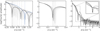 |
Fig. 4 Fourier transforms of synthetic line profiles with positions of the first zero indicated with vertical dotted lines. Left panel: ν sin i parameter is varied from 42 km s−1 (blue) to 90 km s−1 (black) with a step of 6 km s−1 (grey). Middle panel: Linear limb darkening coefficient e is varied from 0.2 (black) to 1.0 (light grey), while ν sin i is kept fixed at 50 km s−1. Right panel: A different contribution of the macroturbulence Θ to the total line broadening is assumed: Θ/v sin i = 0.3, 0.6, 1.2 and 1.8, with ν sin i fixed to 50 km s−1. The inset is a zoom onto the region of the position of the first zero. |
4.3 Inference of the effective temperature Teff and surface gravity log g of the sample stars
As mentioned in Sect. 3, we rely on three grids of synthetic spectra for our analyses. We fit the normalised observed spectra with those predicted by models in the grids by means of a χ2-minimisation to find the best-fit parameters. The fitting is performed in the wavelength range of 4000–5000 Å, which includes a plethora of metal and helium lines, as well as the Ηβ, Ηγ, and Hδ lines. The minimisation is performed with the Trust Region Reflective algorithm (Conn et al. 2000) applied to the  log g− ν sin i parameter space, where the model spectra for the parameter values are interpolated from those in the grids at each step of the iteration. The OSTAR2002 (Lanz & Hubeny 2003) and BSTAR2006 (Lanz & Hubeny 2007) grids of TLUSTY models are employed for the analysis of a few predominantly upper-main sequence stars in the sample. Furthermore, owing to the fact that our sample is dominated by evolved blue supergiants in the LMC with Teff ≳ 10 000 Κ and that the OSTAR2002 and BSTAR2006 grids do not extend towards low log g values characteristic of supergiant stars, we compute a dedicated grid of CMFGEN (Hillier & Miller 1998) models covering log g values as low as 1.7 dex. The parameter space of the grid is dictated by the lowest log g possible for a given Teff such that the star remains in hydrostatic equilibrium. This way, the grid extends from 11 000 Κ to 19 000 Κ in Teff, while logg ranges from 1.7 to 2.5 dex at 11 000 Κ and from 2.2 to 2.5 dex at 19 000 K. Owing to the large computation time, steps of 1000 Κ and 0.1 dex are chosen for Teff and log g, respectively. The parameter space covered with the CMFGEN grid is indicated with the grey shaded area in Fig. 6.
A grid of the local thermodynamic equilibrium (LTE-based) models computed with GSSP code (Tkachenko 2015) is used for the analysis of a few unevolved stars with Teff ≲ 15 000 K, a range in the parameter space not covered by the BSTAR grid of the TLUSTY models and where the use of CMFGEN is not justified. The GSSP grid is designed such that it covers a Teff range between 9000 Κ and 15 000 K. By analogy with the CMFGEN grid and for exactly the same reason (i.e. the star needs to remain in the hydrostatic equilibrium), the log g range is set to 2.5–4.5 dex for Teff < 10 000 Κ and to 3.0–4.5 dex for Teff ≥ 10 000 K. The step in Teff is 100 Κ and 250 Κ for Teff < 10 000 Κ and Teff > 10 000 K, respectively, while the step in log g is fixed to 0.1 dex. We assume the solar chemical composition as derived in Grevesse et al. (2007). This way, we adopt adequate tools for each of the three regimes of stars in our sample. The regions of the parameter space covered by the grids of GSSP, TLUSTY, and CMFGEN models used in this study are illustrated with shaded areas in Fig. 6.
Spectroscopic inference of surface abundances for the sample stars is the subject of a follow-up paper. For this reason, we fix the micro turbulent velocity ξ to 2 km s−1 and 10 km s−1 for all unevolved (GSSP and TLUSTY) and blue supergiant (CMFGEN) models, respectively. Furthermore, we assume solar and about half solar ([M/H] = −0.4 dex) metallicity for all the Galactic and LMC (Choudhury et al. 2021) targets, respectively. The results of the spectroscopic analysis based on this approach are summarised in Table A.1, where the grid of used atmosphere models for a particular target is indicated with superscripts ‘a’, ‘b’, and ‘c’ for GSSP, TLUSTY, and CMFGEN, respectively. The positions of the stars in the spectroscopic  HR diagram are shown in Fig. 6. The v sin i values inferred from this fitting approach (representing the total line broadening) are also provided in Table B.1. As suggested in Sect. 3, the majority of the sample stars are found to be blue supergiants, with just a few objects in their main sequence stage of evolution. We find four objects that have masses in the range between approximately 2.5 and 4.0 M⊙, with three of them being located within the SPB instability region, while the fourth object is found at the border when uncertainties are taken into account. The rest of the stellar sample is consistent with masses in excess of 10 M⊙.
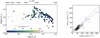 |
Fig. 5 Results of ν sin i inferences. Left panel: positions of the sample stars in the spectroscopic HR diagram. Individual objects are colour coded according to their ν sin i value inferred from the Fourier method. Right panel: comparison of ν sin iSP with ν sin iFT. The grey line shows the case where ν sin iFT and ν sin iSP are equal, while the blue line is an error-weighted fit to the observed values. |
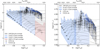 |
Fig. 6 Positions of the sample stars in the spectroscopic log(Teff)–log(ℒ/ℒ⊙) HR diagram. The UVES and FEROS samples are shown with black and blue symbols with error bars, respectively. Regions of the parameter space covered by the GSSP, TLUSTY, and CMFGEN models are marked with red, blue, and grey shaded areas, respectively. Non-rotating mesa stellar evolution tracks computed for Ζ = 0.006 are shown with black solid lines and are taken from Burssens et al. (2020). Left panel: full parameter range. Right panel: zoom onto the high-luminosity region where the bulk of the sample is situated. |
4.4 Inference of the macroturbulent velocity
As discussed in Sect. 4.2, massive stars are known to show macroturbulent velocity fields that are often comparable to or exceed the spectral line broadening associated with the stellar rotation (e.g. Aerts et al. 2014; Simón-Díaz & Herrero 2014; Simón-Díaz et al. 2017). There is currently no consensus as to the exact physical mechanism(s) responsible for the macroturbulent broadening in the spectral lines of massive stars. Two main hypotheses are (i) the collective effect of gravity waves, either heat-driven (Aerts et al. 2009) or stochastically excited at the boundary between the convective core and radiative envelope in these stars (Aerts & Rogers 2015); and (ii) velocity perturbations due to turbulent pressure in the subsurface convection zone driven by the iron opacity peak at some 150 kK (Cantiello et al. 2021). These two hypotheses are not mutually exclusive (Bowman et al. 2020; Bowman & Dorn-Wallenstein 2022).
Our stellar sample is well suited to infer the macroturbulent velocity Θ, as well as to estimate the relative contributions of its radial ΘR and tangential ΘT components. Indeed, we were able to acquire high-resolution, high-S/N, multi-epoch spectroscopic data for the majority of objects in the sample. Furthermore, the sample is composed of stars spanning a wide range of stellar mass (M ∈[3, 80] M⊙) and spectroscopic luminosity (log(ℒ/ℒ⊙) ∈[1.8, 4.5], cf. Fig. 6). Therefore, we proceed with the observational characterisation of the macroturbulent velocity field using synthetic spectra to fit Mg II 4481 Å line profiles. Macroturbulence is treated with a radial-tangential prescription as defined in Takeda & UeNo (2017) for an area element, where a locally broadened profile is defined by a convolution of an intrinsic profile and a macroturbulent kernel:
 (2)
(2)
Here, v stands for the profile velocity from transforming the wavelength with respect to the central wavelength of the line, while θ defines a direction angle into the observer’s line of sight. The quantity K(v, θ) is the convolution kernel due to the macroturbulent broadening and is defined as:
![Mathematical equation: $\matrix{ {K\left( {\upsilon ,\theta } \right) = {{{a_R}} \over {{\pi ^{{1 \mathord{\left/ {\vphantom {1 2}} \right. \kern-\nulldelimiterspace} 2}}}{{\rm{\Theta }}_R}\cos \theta }}\exp \,\left[ { - {{{\upsilon ^2}} \over {{{\left( {{{\rm{\Theta }}_R}\cos \theta } \right)}^2}}}} \right]} \hfill \cr {\,\,\,\,\,\,\,\,\,\,\,\,\,\,\,\,\,\,\,\,\,\,\,\,\,\,\,\,\,\,\,\,\,\,\,\,\,\,\,\,\,\,\,\,\,\,\,\,\,\,\,\,\,\,\,\,\,\, + {{{a_T}} \over {{\pi ^{{1 \mathord{\left/ {\vphantom {1 2}} \right. \kern-\nulldelimiterspace} 2}}}{{\rm{\Theta }}_T}\sin \theta }}\exp \,\left[ { - {{{\upsilon ^2}} \over {{{\left( {{{\rm{\Theta }}_T}\sin \theta } \right)}^2}}}} \right].} \hfill \cr } $](/articles/aa/full_html/2023/08/aa46108-23/aa46108-23-eq5.png) (3)
(3)
The most commonly used approach in the literature to estimate macroturbulence is the one assuming isotropy, that is aR = aT = 0.5 and ΘR = ΘT = Θ.
After convolving the local specific intensities I0(v, θ) with the kernel K(v, θ), the final broadened profile is computed by integrating synthetic specific intensities Ι(μ = cos θ) based on our deduced Teff and log g over the visible sphere for all individual targets. This way, the limb darkening effect is included directly as opposed to the less detailed yet commonly used approach in the literature relying on parametric approximations. In our method, we make the following assumptions: (i) similar to the case of the parameter inference for v sin i, Teff, and log g (cf. Sects. 4.2 and 4.3), we fix the value of the microturbulent velocity to 2 km s−1 and 10 km s−1 for all main sequence and supergiant stars in the sample, respectively; (ii) the v sin i parameter is varied in the range determined by its value and uncertainties inferred with the Fourier-based method (cf. Sect. 4.2); (iii) in the first instance, the macroturbulent parameter Θ is estimated assuming equal contributions of its radial and tangential components (i.e. the isotropic case); and (iv) because specific intensities are not available for the CMFGEN and TLUSTY models, they are calculated from GSSP at the grid node closest to the parameters of the star under consideration. We introduce a line-depth correction factor and apply it to the GSSP model when fitting the observed profile to account for the difference between the GSSP LTE and CMFGEN/TLUSTY non-LTE models. This approach allows us to properly scale the LTE-based intrinsic profile to the expected depth, while any possible difference in the shape of the intrinsic profile between the LTE and non-LTE models is considered negligible compared to the total spectral line broadening due to the combined effect of v sin i, ξ, and Θ.
Figure 7 summarises the obtained results in the form of the distribution of stars in the spectroscopic HR diagram, which is colour coded according to the inferred value of the macroturbulent velocity (left panel), and a histogram of the estimated values (right panel). In the left panel of Fig. 7, one can see a trend of increasing macroturbulent parameter as the effective temperature and spectroscopic luminosity of the star increase. A similar behaviour was previously reported by Simón-Díaz et al. (2017) (their figure 5), who also concluded that stars in the upper part of the spectroscopic HR diagram (M ≥ 15 M⊙) tend to show line profiles with predominantly macroturbulent broadening as opposed to rotational broadening. In the right panel of Fig. 7, one can see that the majority of stars in our sample have a macro-turbulent broadening parameter Θ between some 20 km s−1 and 70 km s−1, with just a few objects being characterised by Θ below or above that range of values. Correcting for the sample size, which in our case is about four times smaller, and for the larger contribution of more evolved objects, the range of the inferred macroturbulent velocity values is consistent with the findings of Simón-Díaz et al. (2017). This is a particularly interesting observation given that the stellar sample analysed by Simón-Díaz et al. (2017) is fully comprised of Galactic objects, while ours is dominated by stars in the LMC, and therefore represents a substantially different metallicity regime.
As a next step, we attempt to estimate the individual contributions of the radial, ΘR, and tangential, ΘT, components of the macroturbulence from an observational viewpoint. In the radial-tangential prescription of macroturbulence, the contribution of the components may be controlled by the parameters aR and aT such that aR + aT = 1. The parameter a may be seen as the relative ratio of cells moving tangentially or radially in a unit area. Methodologically, we expand the parameter vector by aT, where the contribution of the radial component is assumed to be aR = 1− aT. The top panel in Fig. 8 shows the results obtained from the fits, relying on an initial value of 0.5 for aT. The majority of the stars tend to show an equal or more dominant tangential component. The middle and bottom panels of Fig. 8 offer a closer look at the dependence of the obtained results on αT with respect to its assumed initial value. The distributions of aT in the form of histograms and kernel-density estimations (KDE) are shown for three values of its initial guess: aT = 0.25 (yellow), 0.5 (blue), and 0.75 (green). The main conclusions that can be drawn from these distributions are that (i) the peak position correlates with the initial guess assumed for aT; (ii) the peak height decreases in the KDE plot as the initial guess for the aT parameter decreases; (iii) all distributions are skewed towards higher values of aT, where the skewness of the observed distribution is statistically significant as confirmed by a Kolmogorov-Smirnov test with respect to a reference Gaussian distribution centred at the peak of the observed distributions; and (iv) visual inspection of observed profiles reveals that most of the outlying values (aT < 0.4 and aT > 0.8) are due to a high level of noise in the spectra and/or strongly asymmetric line profiles. At the same time, spectra of the best quality in the entire sample tend to show aT/aR ~ 1, where the estimated uncertainty of aT may reach up to 20% for the case treated here.
Furthermore, we compare Θ when aT = 0.5 is fixed and Θ when aT is included as a free parameter and analyse the apparent trends. The comparison (Fig. 9, left panel) illustrates that these Θ are in agreement to within their uncertainties, while the errors increase significantly when aT is varied. There is no obvious trend in the distribution of aT with respect to the value of Θ for aT = 0.5 fixed, as shown in the right panel of Fig. 9.
Finally, following the statistical approach in Aerts et al. (2023), we investigate observed trends in Θ quantitatively from multivariate linear regression models relying on five predictors of the following form:
 (4)
(4)
After consecutive elimination of the insignificant predictors based on the adjusted R2-statistics, taking into account the degrees of freedom, we conclude that the best regression model includes only ν sin i and Teff as relevant predictors, with the following coefficients:
 (5)
(5)
This model explains 96.4% of the observed variability in Θ. We plot the predicted Θ from this regression model together with the observed values for our sample in Fig. 10. There is a clear trend in the ν sin i-Θ plot showing an almost one-to-one correspondence between Θ and ν sin i. Our regression results are remarkably similar to those in the recent study by Aerts et al. (2023), who analysed the correspondence between macro-turbulent broadening and ν sin i for a large sample of ~ 15 000 Galactic gravity-mode pulsators in core-hydrogen burning from low-resolution Gaia DR3 spectra. Moreover, as we mention above in this section, a similar trend between θ and ν sin i was found from high-resolution spectroscopy by Simón-Díaz et al. (2017), who analysed a Galactic sample of Ο and Β stars. As our sample consists mostly of LMC objects and thus represents a significantly lower metallicity regime, it is interesting to compare the results for Θ in our stars with those in the sample of Simón-Díaz et al. (2017) to check if there is any dependence on metallicity. We plot the macroturbulent values from Simón-Díaz et al. (2017) and from our work in Fig. 11. Though the Θ values in the sample of these authors are in general larger for their supergiants than for ours (we note that the first green peak in the right panel corresponds to main sequence stars, which are absent in the LMC sample), the differences remain roughly within the errors of Θ determined for our sample stars. As our sample is populated with more luminous stars, and different methods were used to measure Θ, it is difficult to conclude on whether or not the shift towards lower Θ in our LMC sample has a physical or methodological origin; this situation is made worse by the fact that there are no errors listed for values of the macroturbulent broadening in the study by Simón-Díaz et al. (2017).
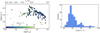 |
Fig. 7 Results of the inference of the macroturbulence parameter Θ. Left panel: stellar positions in the spectroscopic HR diagram colour coded by the inferred value of the macroturbulent velocity parameter Θ. Value of the macroturbulent velocity is an error-weighted average of two epochs. Right panel: distribution of the macroturbulent velocity parameter Θ across the sample. |
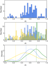 |
Fig. 8 Results of the inference of the tangential component of macro-turbulence. Top panel: Histogram of aT contributions derived from observed profiles of the entire sample with aT = 0.5 as an initial assumption, ν sin i varied within errors of ν sin iFT. Middle panel: Histograms of αT contributions derived from observed profiles of the entire sample with different initial assumptions: 0.25 (yellow), 0.5 (blue), 0.75 (green), and ν sin i left to vary freely. Bottom panel: KDE functions for the same data as in the middle panel. Dashed lines mark initial guesses. The fits demonstrate the results are sensitive to the initial guess. |
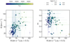 |
Fig. 9 Results of the inference of the tangential component of macro-turbulence. Left panel: comparison of Θ measured with fixed tangential component contribution aT = 0.5 and Θ measured when aT is left to vary freely. Right panel: distribution of tangential component contribution aT over Θ. Colour encodes Teff, while symbol size changes with spectroscopic luminosity. |
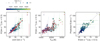 |
Fig. 10 Results of the multivariate linear regression models for Θ. Left panel: comparison between Θ and ν sin i. The colours encode Teff, while the symbol sizes scale with spectroscopic luminosity. The red circles show the predicted Θ value from the best multivariate regression model in Eq. (5) for our LMC sample. The red vertical line in the corner indicates a typical error bar for the predicted Θ values and applies to all three panels. Middle panel: comparison between observed Θ and predictor Teff, where Θ predicted from Eq. (5) is colour coded in red. Right panel: comparison of Θ predicted from Eq. (5) and the measured values of Θ. |
5 Improving the inference of macroturbulence
In the above parameterised estimation of the macroturbulent velocity and of its individual radial and tangential component contributions to the line broadening of our sample stars, we make two fundamental assumptions: (i) the microturbulent velocity ξ is known a priori (e.g. estimated along with Teff and log g of the star or fixed to a value typical for a given spectral type and luminosity class), and (ii) the typical S/N ≃ 100 in the observed spectra is sufficient to distinguish between different line-broadening mechanisms. Although these assumptions are motivated by the most commonly used methodologies and/or empirical evidence in the literature (e.g. Simón-Díaz et al. 2017; Holgado et al. 2018), they may not be valid. To investigate this, we look into the problem in more detail, attempting to identify (i) the requirements in terms of S/N, spectral line selection, and so on for a meaningful inference of the macroturbulent parameter Θ from spectra of Ο and Β stars, (ii) the analysis limitations associated with the parameter correlations, in particular between micro-(ξ) and macro-(Θ)turbulent velocities and rotational broadening ν sin i, and (iii) the conditions under which can one empirically estimate individual contributions of the radial, aR, and tangential, aT, components of the global macroturbulent broadening in the spectra of Ο and Β stars.
The above questions are particularly important to address in light of the high sensitivity of the results obtained in Sect. 4.4 to the initial guess of aT. Moreover, the ability to realistically estimate individual contributions of the radial and tangential components of the macroturbulent broadening is a powerful observational test of various theoretical hypotheses for the origin of macroturbulence as a physical phenomenon. In particular, should wave-driven broadening be at the origin of macroturbulence, one would expect the radial component to dominate over the tangential one in the case of pressure waves, whereas the opposite is true for the case of gravity waves. So far, in the literature, an appreciable effort has been put into estimating the macroturbulent velocity parameter Θ for as many massive stars as possible, and into to searching for possible correlations with various physical mechanisms at work (e.g. Simón-Díaz & Herrero 2014; Simón-Díaz et al. 2017). However, the most common approach is to assume equal contributions of the radial and tangential components, while this choice is the least justified in the case of pulsational broadening (Aerts et al. 2009, 2014).
We simulate synthetic spectra of both a late and an early B-type star, with Teff = 12 000 Κ and log g= 4.0 dex, and Teff = 22 000 Κ and log g = 4.0 dex, respectively, in order to analyse them as they were observed so that we know the exact true parameters and can quantify the deviations of these from inferred parameters. In the case of the late B-type star, we focus on the Mg II 4481 Å spectral line, while we use the Si III 4552 Å, 4557 Å, and 4574 Å triplet in the early B-type star. Spectra are simulated for several combinations of the parameters Θ, ξ, and ν sin i to consider cases where their dominant role is interchanging. Table 1 provides a summary of all the combinations used and we repeat the analysis for three values of S/N = 100, 150, and 250 to address the influence of the quality of observations on the obtained results. At this stage, we assume equal contributions for the radial aR and tangential aT components of the macroturbulence to isolate possible correlations between the Θ, ξ, and ν sin i parameters.
The analysis of all 57 profiles (3 values of S/N and 16 combinations of the Θ and ν sin i parameters with one fixed value of ξ, plus 3 values of S/N and 3 combinations with varied ξ for a fixed pair of Θ and ν sin i) is approached with a Monte Carlo formalism. That is, each simulated profile (in other words, each combination of input parameters) is fitted multiple (200) times, where each new fit is done after applying normally distributed noise to the simulated profile. The fitting is being performed by minimising a χ2 merit function between the noisy synthetic profile and the grid of synthetic profiles covering the full parameter space. Such simulations allow quantitative estimation of the effect of the S/N on the spread of the estimated parameters around their true value, as well as assessment of their correlations.
Figure 12 illustrates a simplified case where υ sin i is fixed (under the assumption that it can be determined from an independent method, such as the one based on the FT). The minimisation is performed for only two parameters, namely the micro- and macroturbulent velocities (ξ and Θ). Similar figures for other combinations with Teff = 12000 Κ (Mg II) are presented in Appendix C (Figs C.1–C.11). Plots for the case of Teff = 22 000 K and the Si III diagnostic line are left out as they show the same trends. For a given value of the v sin i parameter and quality of the observed spectrum characterised by its S/N value, we find a strong correlation between ξ and Θ. Moreover, the correlation persists irrespective of whether the rotational broadening dominates over the macroturbulent broadening (top versus bottom row in Fig. 12). Furthermore, the 1σ, 2σ, and 3σ uncertainty intervals for ξ and Θ are a strong function of the S/N value in the observed spectrum of the star (left, middle, and right columns in Fig. 12). In particular, irrespective of the assumed effective temperature of the star and accounting for the parameter correlations, we find that at the 2σ level: (i) Θ can be inferred with a typical precision ranging from approximately 40% to 100% at S/N ≃ 150 and 100, respectively, and better than approximately 30% at S/N ≃ 250 when the rotational broadening dominates over macroturbulence; (ii) Θ can be inferred with a precision of better than 50%, 30%, and 10% at S/N ≃ 100, 150, and 250, respectively, when the contributions from rotational broadening and macroturbulence are equal; and (iii) Θ can be inferred with a precision of approximately 20%, 10%, and 5% at S/N ≃ 100, 150, and 250, respectively, when macroturbulence dominates over rotational broadening.
As the described test was performed with the assumption of v sin i being known precisely, which is never the case, we now repeat the above test with one of the combinations of ξ and Θ including optimisation of the third free parameter, v sin i, allowing it to vary within the typical range of uncertainty of the FT method (10%). The result is shown in Fig. C.12. One can see that v sin i is not significantly correlated with either ξ or Θ but introduces a spread of up to 100% in Θ, even in the case where it is varied in a limited range. We note that v sin i dominates over Θ in this instance of the test, which confirms that the determination of Θ is unreliable unless it dominates over v sin i.
As a further test, we now also include a tangential component of macroturbulence, aT, as another free parameter and allow v sin i to vary. This implies we use four free parameters when fitting the line profiles: v sin i, ξ, Θ, and aT. The result is shown in Fig. C.13 for the case of S/N = 250. The main conclusion is that even at such high S/N, one can barely distinguish between a fit with equal radial and tangential contributions (aT = 0.5) and a fit with complete dominance of the tangential component (aT = 1.0) at 1σ confidence level. When allowing a 3σ confidence level, the solution space covers the entire range from 0 to 1 for aT. Thus, line profiles of lower S/N do not allow us to constrain this parameter observationally when independent constraints on other parameters are unavailable.
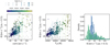 |
Fig. 11 Comparison of Θ observed in our sample and Θ for the sample treated by Simón-Díaz et al. (2017). Circles show the results for our LMC stars, while triangles are the results from Simón-Díaz et al. (2017) for their sample of Ο and Β stars in the Galaxy. Left panel: comparison between observed Θ and ν sin i with the same colour and symbol scheme for Teff as in Fig. 10. Middle panel: comparison between observed Θ and Teff. Right panel: comparison of histograms and KDE for Θ in our sample (blue) and the one of Simón-Díaz et al. (2017; green). |
Combinations of the Θ, ξ, and ν sin i parameter values used in the analysis of spectral line broadening due to the macroturbulent velocity and its interplay with the two other broadening mechanisms.
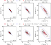 |
Fig. 12 Results of Monte Carlo simulations on synthetic profiles of Mg II (top set of panels) and Si III (bottom set of panels) with artificial noise (left panels: S/N = 250, middle panels: S/N = 150, and right panels: S/N = 100) with 1σ, 2σ, and 3σ confidence ellipses. Correlation coefficients ρ are indicated in the right corner of each panel. v sin i is fixed, while ξ and Θ are optimised. The red crosses mark true parameters of the synthetic profiles. |
6 Discussion and conclusions
In this first paper of the series, we present a study of 124 O and B stars with unique catalogue identifiers from two ESO large programmes that employ the high-resolution FEROS and UVES instruments. The sample is mostly composed of supergiants in the LMC and a few dwarfs in the Galaxy. All stars in our sample are found in the CVZ-S of the TESS space telescope, and thanks to the 1 yr time base of photometric observations, they are potential candidates for future asteroseismic modelling (Garcia et al. 2022a,b). The same argument applies to the 124 Galactic dwarf stars analysed in detail in the complementary study by Gebruers et al. (2022).
We find that the reduced spectra delivered by the ESO pipeline do not meet our stringent requirements in terms of precision of the spectroscopically inferred atmospheric parameters for future asteroseismic modelling. Therefore, we developed a custom normalisation of the obtained spectra starting from the intermediate data product resulting from the ESO pipeline, that is the blaze-corrected non-merged wavelength-calibrated spectra. Our tests show that a rather simple recipe of order-by-order normalisation works well for the blue supergiants in our sample. However, for dwarfs, the same recipe fails to provide high-quality spectrum normalisation, most notably in the wavelength regions of the broad hydrogen lines. For those, we developed an even more sophisticated spectrum normalisation method that relies on a grid of synthetic spectra. The latter allows us to locate the local continuum and approximates the normalisation function with a series of Chebyshev polynomials.
We employ the LSD method to compute high-S/N average profiles for all epochs and for all the stars in our sample. We fit the obtained LSD profiles with asymmetric Gaussian functions to deduce radial velocities and the degree of asymmetry of the line profiles for each epoch. The inferred information is employed to perform a spectroscopic variability classification of the stars, where we consider four variability classes: apparently constant (‘const’), spectroscopic binaries (‘SB’), stars showing line profiles variations (‘LPV’), and stars with line profiles characterised by an appreciable degree of skewness (‘asymm’). Considering the UVES and FEROS samples separately, we find 86 apparently constant stars, 7 stars showing LPV, 28 spectroscopic binary candidates, and 37 stars exhibiting asymmetric line pro-files9. Out of 24 stars that have both UVES and FEROS data, 20 are assigned to the same variability class. The remaining four stars, HD 268653, HD 269145, HD 269766, and HD 268675, are either classified as apparently constant based on one data set and tentatively variable in the other one, or have an extra class assignment based on either data set (see Table A.1 for details). Finally, 24 classifications are tentative and more spectroscopic epochs are required for an unambiguous class assignment.
The positions of the sample stars in the spectroscopic HR diagram lead to the majority of them being identified as blue supergiants, with only a few objects being dwarfs situated within the SPB and β Cep instability regions. Detailed analyses of all available sectors of TESS space-based photometry are beyond the scope of this initial spectroscopy paper but will be presented in follow-up publications. Nevertheless, we performed a cross-match of our sample with the O- and B-type stars studied in Bowman et al. (2019a, 2020). In the observed sample, for 80% of the blue supergiants situated outside the instability regions in Fig. 6, these authors report SLF variability. One of those objects was reported to show heat-driven oscillations in TESS photometry. Only 3 of 10 stars situated within the instability regions from our spectroscopic parameters show oscillations. Validation of these initial photometric results from all available TESS sector data will be carried out in a dedicated follow-up study.
We employ two different methods to infer the projected rotational velocities v sin i from the spectra of the sample stars: one based on the FT of line profiles and the other one from fitting synthetic spectra to selected line profiles. Owing to the diversity of mechanisms causing the total line broadening in early-type stars, we find that the method of synthetic spectra delivers v sin i values that are either comparable to or exceed those inferred with the FT method. Therefore, we accept the FT-based v sin i measurements as the final and most precise ones in our study (see Table B.1, column “v sin iFT”) and recommend their use instead of those inferred from the method of synthetic spectra.
The v sin i values resulting from the FT method are subsequently used to quantify the amount of spectral line broadening due to macroturbulence for all stars in the sample. In the process, we allow v sin i to vary in a narrow range dictated by its uncertainty. We find a tendency for the macroturbulent parameter Θ to increase as the effective temperature and spectroscopic luminosity of the star increase, and that the majority of stars in the sample show macroturbulent broadening in the range between approximately 20 km s−1 and 70 km s−1. Both these findings are in agreement with the results of Simón-Díaz et al. (2017), which are based on 430 Galactic massive stars of spectral types O and B. Given that the majority of the stars in our sample are in the LMC, which is characterised by a significantly lower metallicity than the Galactic sample in Simón-Díaz et al. (2017), we conclude that the observed macroturbulence in the spectral lines of massive stars does not depend on their bulk metallicity (taking into account our smaller sample size and its dominance by evolved objects). Furthermore, we check for a possible correlation between the inferred macroturbulent velocity parameter and the variability class we have assigned to our targets (cf. Table A.1). In this exercise, we consider the following groups of stars: (i)‘const’ versus all other groups together, (ii) ‘const’ versus ‘asymm’, (iii) ‘const’ versus ‘LPV’, and (iv) ‘asymm’ versus ‘LPV’. We could not identify any correlation between the macroturbulent velocity and the class of spectroscopic variability.
In an attempt to quantify the two individual contributions known as the radial and tangential components of macroturbulence from spectral line fitting, we find the results to be sensitive to the initial guess for the respective parameters aR and aT10. Although the obtained distribution is skewed towards aT ≳ 0.6, we cannot firmly conclude that we observe a dominant tangential component given the limited quality of our spectroscopic data in terms of S/N. When all the assumptions of our approach are met, namely (i) a fixed microturbulent velocity ξ applies that is typical of a given spectral type; (ii) the v sin i inferred from Fourier transforms of the observed profiles varies modestly; and (iii) the initial guess for aT is not lower than 0.4, one may conclude that the tangential component aT is larger than the radial one in our sample. This may possibly be an indicator of broadening by gravity or gravito-inertial waves (Aerts et al. 2023). This interpretation should be treated with caution because any meaningful inference for the individual radial and tangential components of the macroturbulent broadening requires S/N ≥ 250 (see Sect. 5).
Finally, we add a word of caution that refers to the way uncertainties are estimated for the macroturbulent velocity parameter Θ in the literature. The commonly accepted approach, and the one taken in this work, is to decouple the inferences of the macro- and microturbulent broadening parameters, where the latter is usually optimised together with the effective temperature and surface gravity of the star. Our study shows that the Θ and ξ parameters are strongly correlated for the case of massive stars. Hence, fixing the microturbulent velocity parameter ξ while quantifying the contribution of macroturbulence to the line broadening results in underestimation of the uncertainties for the latter. Furthermore, the precision with which the macroturbulent broadening parameter Θ can be inferred depends strongly on the S/N of the spectra, as well as on the dominant line broadening mechanism among rotation or macroturbulence. The uncertainty on the Θ parameter increases progressively as the dominance of the projected rotational velocity v sin i grows. These findings are in agreement with the results obtained by Simón-Díaz et al. (2017), where the authors report only the upper limit for the macroturbulence parameter for the majority of stars with v sin i > Θ.
Future studies of all stars in the combined UVES and FEROS samples will be focused on detailed analyses of their atmospheric chemical compositions and frequency analyses based on all TESS data available at the time. Subsequently, we will also perform detailed asteroseismic modelling for stars with sufficient identified oscillation modes, relying on the spectroscopic constraints provided by this work and from the future results for the individual elemental abundances.
Acknowledgements
The research leading to these results has received funding from the KU Leuven Research Council (grant C16/18/005: PARADISE), from the Research Foundation Flanders (FWO) under grant agreements G089422N (NS, CA, AT), K802922N (CA, Sabbatical leave), 11E5620N (SG, PhD Aspirant mandate), 1124321N (LIJ, PhD Aspirant mandate), 12ZB620N (TVR, Junior Postdoctoral Fellowship), and 1286521N (DMB, Senior Postdoctoral Fellowship), as well as from the BELgian federal Science Policy Office (BELSPO) through PRODEX grant PLATO. The research is based on observations collected at the European Southern Observatory under ESO programs 1104.D-0230 and 0104.A-9001. This research has made use of the SIMBAD database, operated at CDS, Strasbourg, France. The TESS data presented in this paper were obtained from the Mikulski Archive for Space Telescopes (MAST) at the Space Telescope Science Institute (STScI), which is operated by the Association of Universities for Research in Astronomy, Inc., under NASA contract NAS5-26555. Support to MAST for these data is provided by the NASA Office of Space Science via grant NAG5-7584 and by other grants and contracts. Funding for the TESS mission is provided by the NASA Explorer Program.
Appendix A Results of the global stellar parameter estimations
Results of the spectrum analysis and respective spectroscopic classification of stars in the combined UVES and FEROS sample.
Appendix B Results of spectral line profiles characterisation
Characteristics of the spectral line profile broadening in the combined UVES and FEROS sample.
Appendix C Results of Monte Carlo simulations of broadened line profiles
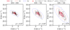 |
Fig. C.1 Results of Monte Carlo simulations on synthetic profiles of Mg II 4481 Å line with artificial noise (left panel: S/N = 250, middle panel: S/N = 150, and right panel: S/N = 100) with 1, 2, and 3σ confidence ellipses. Correlation coefficients ρ are indicated in the right corner of each panel, υ sin i is fixed, while Θ and ξ are optimised. The red crosses mark the true parameters of the synthetic profiles. |
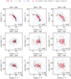 |
Fig. C.12 Same as Fig. C.1 but v sin i is optimised as well as ξ and Θ, resulting in three free parameters. |
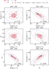 |
Fig. C.13 Same as Fig. C.1 but v sin i and aT are optimised as well as ξ and Θ, resulting in four free parameters. Only the results for S/N=250 are shown. |
References
- Aerts, C. 2021, Rev. Mod. Phys., 93, 015001 [Google Scholar]
- Aerts, C., & Kolenberg, K. 2005, A&A, 431, 615 [NASA ADS] [CrossRef] [EDP Sciences] [Google Scholar]
- Aerts, C., & Rogers, T. M. 2015, ApJ, 806, L33 [Google Scholar]
- Aerts, C., De Cat, P., Peeters, E., et al. 1999, A&A, 343, 872 [NASA ADS] [Google Scholar]
- Aerts, C., Thoul, A., Daszyńska, J., et al. 2003, Science, 300, 1926 [Google Scholar]
- Aerts, C., Puls, J., Godart, M., & Dupret, M. A. 2009, A&A, 508, 409 [NASA ADS] [CrossRef] [EDP Sciences] [Google Scholar]
- Aerts, C., Christensen-Dalsgaard, J., & Kurtz, D. W. 2010a, Asteroseismology, Astronomy and Astrophysics Library (Springer Science+Business Media) [Google Scholar]
- Aerts, C., Lefever, K., Baglin, A., et al. 2010b, A&A, 513, A11 [NASA ADS] [CrossRef] [EDP Sciences] [Google Scholar]
- Aerts, C., Briquet, M., Degroote, P., Thoul, A., & van Hoolst, T. 2011, A&A, 534, A98 [NASA ADS] [CrossRef] [EDP Sciences] [Google Scholar]
- Aerts, C., Simón-Díaz, S., Groot, P. J., & Degroote, P. 2014, A&A, 569, A118 [NASA ADS] [CrossRef] [EDP Sciences] [Google Scholar]
- Aerts, C., Símon-Díaz, S., Bloemen, S., et al. 2017a, A&A, 602, A32 [NASA ADS] [CrossRef] [EDP Sciences] [Google Scholar]
- Aerts, C., Van Reeth, T., & Tkachenko, A. 2017b, ApJ, 847, L7 [Google Scholar]
- Aerts, C., Bowman, D. M., Símon-Díaz, S., et al. 2018, MNRAS, 476, 1234 [NASA ADS] [CrossRef] [Google Scholar]
- Aerts, C., Mathis, S., & Rogers, T. M. 2019, ARA&A, 57, 35 [Google Scholar]
- Aerts, C., Molenberghs, G., & De Ridder, J. 2023, A&A, 672, A183 [NASA ADS] [CrossRef] [EDP Sciences] [Google Scholar]
- Auvergne, M., Bodin, P., Boisnard, L., et al. 2009, A&A, 506, 411 [NASA ADS] [CrossRef] [EDP Sciences] [Google Scholar]
- Balona, L. A. 2014, MNRAS, 437, 1476 [NASA ADS] [CrossRef] [Google Scholar]
- Balona, L. A., & Ozuyar, D. 2020, MNRAS, 493, 5871 [CrossRef] [Google Scholar]
- Balona, L. A., Daszynska-Daszkiewicz, J., & Pamyatnykh, A. A. 2015, MNRAS, 452, 3073 [NASA ADS] [CrossRef] [Google Scholar]
- Beck, P. G., Montalban, J., Kallinger, T., et al. 2012, Nature, 481, 55 [Google Scholar]
- Belkacem, K., Samadi, R., Goupil, M.-J., et al. 2009, Science, 324, 1540 [NASA ADS] [CrossRef] [Google Scholar]
- Belkacem, K., Dupret, M. A., & Noels, A. 2010, A&A, 510, A6 [NASA ADS] [CrossRef] [EDP Sciences] [Google Scholar]
- Blomme, R., Mahy, L., Catala, C., et al. 2011, A&A, 533, A4 [NASA ADS] [CrossRef] [EDP Sciences] [Google Scholar]
- Borucki, W. J., Koch, D., Basri, G., et al. 2010, Science, 327, 977 [Google Scholar]
- Bouabid, M. P., Dupret, M. A., Salmon, S., et al. 2013, MNRAS, 429, 2500 [Google Scholar]
- Bowman, D. M. 2020, Front. Astron. Space Sci., 7, 70 [Google Scholar]
- Bowman, D. M., & Dorn-Wallenstein, T. Z. 2022, A&A, 668, A134 [NASA ADS] [CrossRef] [EDP Sciences] [Google Scholar]
- Bowman, D. M., & Kurtz, D. W. 2018, MNRAS, 476, 3169 [NASA ADS] [CrossRef] [Google Scholar]
- Bowman, D. M., & Michielsen, M. 2021, A&A, 656, A158 [NASA ADS] [CrossRef] [EDP Sciences] [Google Scholar]
- Bowman, D. M., Burssens, S., Pedersen, M. G., et al. 2019a, Nat. Astron., 3, 760 [Google Scholar]
- Bowman, D. M., Johnston, C., Tkachenko, A., et al. 2019b, ApJ, 883, L26 [Google Scholar]
- Bowman, D. M., Aerts, C., Johnston, C., et al. 2019c, A&A, 621, A135 [NASA ADS] [CrossRef] [EDP Sciences] [Google Scholar]
- Bowman, D. M., Burssens, S., Simón-Díaz, S., et al. 2020, A&A, 640, A36 [NASA ADS] [CrossRef] [EDP Sciences] [Google Scholar]
- Brahm, R., Jordán, A., & Espinoza, N. 2017, PASP, 129, 034002 [Google Scholar]
- Briquet, M., Aerts, C., Baglin, A., et al. 2011, A&A, 527, A112 [CrossRef] [EDP Sciences] [Google Scholar]
- Briquet, M., Neiner, C., Aerts, C., et al. 2012, MNRAS, 427, 483 [NASA ADS] [CrossRef] [Google Scholar]
- Burssens, S., Simón-Díaz, S., Bowman, D. M., et al. 2020, A&A, 639, A81 [NASA ADS] [CrossRef] [EDP Sciences] [Google Scholar]
- Buysschaert, B., Aerts, C., Bloemen, S., et al. 2015, MNRAS, 453, 89 [NASA ADS] [CrossRef] [Google Scholar]
- Buysschaert, B., Aerts, C., Bowman, D. M., et al. 2018, A&A, 616, A148 [NASA ADS] [CrossRef] [EDP Sciences] [Google Scholar]
- Cantiello, M., Langer, N., Brott, I., et al. 2009, A&A, 499, 279 [NASA ADS] [CrossRef] [EDP Sciences] [Google Scholar]
- Cantiello, M., Mankovich, C., Bildsten, L., Christensen-Dalsgaard, J., & Paxton, B. 2014, ApJ, 788, 93 [Google Scholar]
- Cantiello, M., Lecoanet, D., Jermyn, A. S., & Grassitelli, L. 2021, ApJ, 915, 112 [NASA ADS] [CrossRef] [Google Scholar]
- Carroll, J. A. 1933, MNRAS, 93, 478 [NASA ADS] [CrossRef] [Google Scholar]
- Cheng, S. J., Fuller, J., Guo, Z., Lehman, H., & Hambleton, K. 2020, ApJ, 903, 122 [NASA ADS] [CrossRef] [Google Scholar]
- Choudhury, S., de Grijs, R., Bekki, K., et al. 2021, MNRAS, 507, 4752 [CrossRef] [Google Scholar]
- Claret, A., & Bloemen, S. 2011, A&A, 529, A75 [NASA ADS] [CrossRef] [EDP Sciences] [Google Scholar]
- Claret, A., & Torres, G. 2018, ApJ, 859, 100 [Google Scholar]
- Claret, A., & Torres, G. 2019, ApJ, 876, 134 [Google Scholar]
- Conn, A. R., Gould, N. I. M., & Toint, P. L. 2000, Trust Region Methods (Society for Industrial and Applied Mathematics) [CrossRef] [Google Scholar]
- Deal, M., Richard, O., & Vauclair, S. 2016, A&A, 589, A140 [NASA ADS] [CrossRef] [EDP Sciences] [Google Scholar]
- Deal, M., Escobar, M. E., Vauclair, S., et al. 2017, A&A, 601, A127 [NASA ADS] [CrossRef] [EDP Sciences] [Google Scholar]
- De Cat, P., & Aerts, C. 2002, A&A, 393, 965 [NASA ADS] [CrossRef] [EDP Sciences] [Google Scholar]
- Degroote, P., Briquet, M., Catala, C., et al. 2009, A&A, 506, 111 [NASA ADS] [CrossRef] [EDP Sciences] [Google Scholar]
- Degroote, P., Aerts, C., Baglin, A., et al. 2010a, Nature, 464, 259 [Google Scholar]
- Degroote, P., Briquet, M., Auvergne, M., et al. 2010b, A&A, 519, A38 [NASA ADS] [CrossRef] [EDP Sciences] [Google Scholar]
- Deheuvels, S., Brandão, I., Silva Aguirre, V., et al. 2016, A&A, 589, A93 [NASA ADS] [CrossRef] [EDP Sciences] [Google Scholar]
- Deheuvels, S., Ballot, J., Eggenberger, P., et al. 2020, A&A, 641, A117 [EDP Sciences] [Google Scholar]
- Dekker, H., D’Odorico, S., Kaufer, A., Delabre, B., & Kotzlowski, H. 2000, SPIE Conf. Ser., 4008, 534 [Google Scholar]
- Diago, P. D., Gutiérrez-Soto, J., Auvergne, M., et al. 2009, A&A, 506, 125 [NASA ADS] [CrossRef] [EDP Sciences] [Google Scholar]
- Donati, J. F., Semel, M., Carter, B. D., Rees, D. E., & Collier Cameron, A. 1997, MNRAS, 291, 658 [Google Scholar]
- Dziembowski, W. A., & Pamyatnykh, A. A. 2008, MNRAS, 385, 2061 [NASA ADS] [CrossRef] [Google Scholar]
- Edelmann, P. V. F., Ratnasingam, R. P., Pedersen, M. G., et al. 2019, ApJ, 876, 4 [NASA ADS] [CrossRef] [Google Scholar]
- Freudling, W., Romaniello, M., Bramich, D. M., et al. 2013, A&A, 559, A96 [NASA ADS] [CrossRef] [EDP Sciences] [Google Scholar]
- Fuller, J. 2017, MNRAS, 472, 1538 [Google Scholar]
- Fuller, J. 2021, MNRAS, 501, 483 [Google Scholar]
- Fuller, J., & Lai, D. 2012, MNRAS, 420, 3126 [NASA ADS] [CrossRef] [Google Scholar]
- Fuller, J., Hambleton, K., Shporer, A., Isaacson, H., & Thompson, S. 2017, MNRAS, 472, L25 [Google Scholar]
- Fuller, J., Kurtz, D. W., Handler, G., & Rappaport, S. 2020, MNRAS, 498, 5730 [NASA ADS] [CrossRef] [Google Scholar]
- Gaia Collaboration (De Ridder, J., et al.) 2023, A&A, 674, A36 [CrossRef] [EDP Sciences] [Google Scholar]
- Garcia, S., Van Reeth, T., De Ridder, J., & Aerts, C. 2022a, A&A, 668, A137 [NASA ADS] [CrossRef] [EDP Sciences] [Google Scholar]
- Garcia, S., Van Reeth, T., De Ridder, J., et al. 2022b, A&A, 662, A82 [NASA ADS] [CrossRef] [EDP Sciences] [Google Scholar]
- Gebruers, S., Tkachenko, A., Bowman, D., et al. 2022, A&A, 665, A36 [NASA ADS] [CrossRef] [EDP Sciences] [Google Scholar]
- Gray, D. F. 2008, The Observation and Analysis of Stellar Photospheres (Cambridge, UK: Cambridge University Press) [Google Scholar]
- Gray, R. O., & Corbally, Christopher, J. 2009, Stellar Spectral Classification (Princeton University Press) [CrossRef] [Google Scholar]
- Grevesse, N., Asplund, M., & Sauval, A. J. 2007, Space Sci. Rev., 130, 105 [Google Scholar]
- Guo, Z. 2021, Front. Astron. Space Sci., 8, 67 [NASA ADS] [Google Scholar]
- Guo, Z., Fuller, J., Shporer, A., et al. 2019, ApJ, 885, 46 [Google Scholar]
- Guo, Z., Shporer, A., Hambleton, K., & Isaacson, H. 2020, ApJ, 888, 95 [Google Scholar]
- Gutiérrez-Soto, J., Floquet, M., Samadi, R., et al. 2009, A&A, 506, 133 [NASA ADS] [CrossRef] [EDP Sciences] [Google Scholar]
- Hambleton, K. M., Kurtz, D. W., Prša, A., et al. 2013, MNRAS, 434, 925 [Google Scholar]
- Hambleton, K., Kurtz, D. W., Prša, A., et al. 2016, MNRAS, 463, 1199 [Google Scholar]
- Handler, G., Jerzykiewicz, M., Rodríguez, E., et al. 2006, MNRAS, 365, 327 [NASA ADS] [CrossRef] [Google Scholar]
- Handler, G., Matthews, J. M., Eaton, J. A., et al. 2009, ApJ, 698, L56 [NASA ADS] [CrossRef] [Google Scholar]
- Handler, G., Kurtz, D. W., Rappaport, S. A., et al. 2020, Nat. Astron., 4, 684 [Google Scholar]
- Hekker, S., & Christensen-Dalsgaard, J. 2017, A&ARv, 25, 1 [Google Scholar]
- Hermes, J. J., Gänsicke, B. T., Kawaler, S. D., et al. 2017, ApJS, 232, 23 [Google Scholar]
- Hillier, D. J., & Miller, D. L. 1998, ApJ, 496, 407 [NASA ADS] [CrossRef] [Google Scholar]
- Holgado, G., Simón-Díaz, S., Barbá, R. H., et al. 2018, A&A, 613, A65 [NASA ADS] [CrossRef] [EDP Sciences] [Google Scholar]
- Horst, L., Edelmann, P. V. F., Andrássy, R., et al. 2020, A&A, 641, A18 [NASA ADS] [CrossRef] [EDP Sciences] [Google Scholar]
- Huat, A. L., Hubert, A. M., Baudin, F., et al. 2009, A&A, 506, 95 [NASA ADS] [CrossRef] [EDP Sciences] [Google Scholar]
- Hunter, I., Lennon, D. J., Dufton, P. L., et al. 2008, A&A, 479, 541 [NASA ADS] [CrossRef] [EDP Sciences] [Google Scholar]
- IJspeert, L. W., Tkachenko, A., Johnston, C., et al. 2021, A&A, 652, A120 [NASA ADS] [CrossRef] [EDP Sciences] [Google Scholar]
- Jayaraman, R., Handler, G., Rappaport, S. A., et al. 2022, ApJ, 928, L14 [NASA ADS] [CrossRef] [Google Scholar]
- Johnston, C. 2021, A&A, 655, A29 [NASA ADS] [CrossRef] [EDP Sciences] [Google Scholar]
- Kaufer, A., Stahl, O., Tubbesing, S., et al. 1999, The Messenger, 95, 8 [Google Scholar]
- Kołaczek-Szymanski, P. A., Pigulski, A., Michalska, G., MoZdzierski, D., & Rózański, T. 2021, A&A, 647, A12 [NASA ADS] [CrossRef] [EDP Sciences] [Google Scholar]
- Kurtz, D. W. 2022, ARA&A, 60, 31 [NASA ADS] [CrossRef] [Google Scholar]
- Kurtz, D. W., Handler, G., Rappaport, S. A., et al. 2020, MNRAS, 494, 5118 [Google Scholar]
- Lampens, P. 2021, Galaxies, 9, 28 [NASA ADS] [CrossRef] [Google Scholar]
- Lanz, T., & Hubeny, I. 2003, ApJS, 146, 417 [NASA ADS] [CrossRef] [Google Scholar]
- Lanz, T., & Hubeny, I. 2007, ApJS, 169, 83 [CrossRef] [Google Scholar]
- Lecoanet, D., Cantiello, M., Quataert, E., et al. 2019, ApJ, 886, L15 [Google Scholar]
- Lecoanet, D., Bowman, D. M., & Van Reeth, T. 2022, MNRAS, 512, L16 [NASA ADS] [CrossRef] [Google Scholar]
- Lee, J. W. 2021, PASJ, 73, 809 [NASA ADS] [CrossRef] [Google Scholar]
- Li, G., Van Reeth, T., Bedding, T. R., et al. 2020, MNRAS, 491, 3586 [Google Scholar]
- Maceroni, C., Montalbán, J., Michel, E., et al. 2009, A&A, 508, 1375 [NASA ADS] [CrossRef] [EDP Sciences] [Google Scholar]
- Mahy, L., Gosset, E., Baudin, F., et al. 2011, A&A, 525, A101 [CrossRef] [EDP Sciences] [Google Scholar]
- Mahy, L., Almeida, L. A., Sana, H., et al. 2020a, A&A, 634, A119 [NASA ADS] [CrossRef] [EDP Sciences] [Google Scholar]
- Mahy, L., Sana, H., Abdul-Masih, M., et al. 2020b, A&A, 634, A118 [NASA ADS] [CrossRef] [EDP Sciences] [Google Scholar]
- Martins, F., & Palacios, A. 2013, A&A, 560, A16 [NASA ADS] [CrossRef] [EDP Sciences] [Google Scholar]
- Maxted, P. F. L., & Hutcheon, R. J. 2018, A&A, 616, A38 [NASA ADS] [CrossRef] [EDP Sciences] [Google Scholar]
- Maxted, P. F. L., Gaulme, P., Graczyk, D., et al. 2020, MNRAS, 498, 332 [Google Scholar]
- Michielsen, M., Pedersen, M. G., Augustson, K. C., Mathis, S., & Aerts, C. 2019, A&A, 628, A76 [NASA ADS] [CrossRef] [EDP Sciences] [Google Scholar]
- Michielsen, M., Aerts, C., & Bowman, D. M. 2021, A&A, 650, A175 [NASA ADS] [CrossRef] [EDP Sciences] [Google Scholar]
- Miglio, A., Montalbán, J., Noels, A., & Eggenberger, P. 2008, MNRAS, 386, 1487 [Google Scholar]
- Mombarg, J. S. G., Van Reeth, T., Pedersen, M. G., et al. 2019, MNRAS, 485, 3248 [NASA ADS] [CrossRef] [Google Scholar]
- Mombarg, J. S. G., Dotter, A., Van Reeth, T., et al. 2020, ApJ, 895, 51 [Google Scholar]
- Mombarg, J. S. G., Van Reeth, T., & Aerts, C. 2021, A&A, 650, A58 [NASA ADS] [CrossRef] [EDP Sciences] [Google Scholar]
- Mombarg, J. S. G., Dotter, A., Rieutord, M., et al. 2022, ApJ, 925, 154 [NASA ADS] [CrossRef] [Google Scholar]
- Moravveji, E., Aerts, C., Pápics, P. I., Triana, S. A., & Vandoren, B. 2015, A&A, 580, A27 [NASA ADS] [CrossRef] [EDP Sciences] [Google Scholar]
- Moravveji, E., Townsend, R. H. D., Aerts, C., & Mathis, S. 2016, ApJ, 823, 130 [NASA ADS] [CrossRef] [Google Scholar]
- Mosser, B., Goupil, M. J., Belkacem, K., et al. 2012, A&A, 548, A10 [NASA ADS] [CrossRef] [EDP Sciences] [Google Scholar]
- Mowlavi, N., Barblan, F., Saesen, S., & Eyer, L. 2013, A&A, 554, A108 [NASA ADS] [CrossRef] [EDP Sciences] [Google Scholar]
- Mowlavi, N., Saesen, S., Semaan, T., et al. 2016, A&A, 595, A1 [NASA ADS] [CrossRef] [EDP Sciences] [Google Scholar]
- Moździerski, D., Pigulski, A., Kopacki, G., Kołaczkowski, Z., & Stęślicki, M. 2014, Acta Astron., 64, 89 [NASA ADS] [Google Scholar]
- Moźsdzierski, D., Pigulski, A., Kołaczkowski, Z., et al. 2019, A&A, 632, A95 [NASA ADS] [CrossRef] [EDP Sciences] [Google Scholar]
- Murphy, S. J., Hey, D., Van Reeth, T., & Bedding, T. R. 2019, MNRAS, 485, 2380 [NASA ADS] [CrossRef] [Google Scholar]
- Neiner, C., Gutiérrez-Soto, J., Baudin, F., et al. 2009, A&A, 506, 143 [NASA ADS] [CrossRef] [EDP Sciences] [Google Scholar]
- Neiner, C., Mathis, S., Saio, H., et al. 2012, A&A, 539, A90 [NASA ADS] [CrossRef] [EDP Sciences] [Google Scholar]
- Ouazzani, R.-M., Salmon, S. J. A. J., Antoci, V., et al. 2017, MNRAS, 465, 2294 [Google Scholar]
- Ouazzani, R. M., Marques, J. P., Goupil, M. J., et al. 2019, A&A, 626, A121 [NASA ADS] [CrossRef] [EDP Sciences] [Google Scholar]
- Ouazzani, R. M., Lignières, F., Dupret, M. A., et al. 2020, A&A, 640, A49 [NASA ADS] [CrossRef] [EDP Sciences] [Google Scholar]
- Pápics, P. I., Tkachenko, A., Van Reeth, T., et al. 2017, A&A, 598, A74 [Google Scholar]
- Pavlovski, K., Hummel, C. A., Tkachenko, A., et al. 2022, A&A, 658, A92 [NASA ADS] [CrossRef] [EDP Sciences] [Google Scholar]
- Pedersen, M. G. 2022, ApJ, 930, 94 [NASA ADS] [CrossRef] [Google Scholar]
- Pedersen, M. G., Aerts, C., Pápics, P. I., & Rogers, T. M. 2018, A&A, 614, A128 [NASA ADS] [CrossRef] [EDP Sciences] [Google Scholar]
- Pedersen, M. G., Chowdhury, S., Johnston, C., et al. 2019, ApJ, 872, L9 [Google Scholar]
- Pedersen, M. G., Aerts, C., Pápics, P. I., et al. 2021, Nat. Astron., 5, 715 [NASA ADS] [CrossRef] [Google Scholar]
- Rappaport, S. A., Kurtz, D. W., Handler, G., et al. 2021, MNRAS, 503, 254 [NASA ADS] [Google Scholar]
- Ratnasingam, R. P., Edelmann, P. V. F., & Rogers, T. M. 2020, MNRAS, 497, 4231 [NASA ADS] [CrossRef] [Google Scholar]
- Ricker, G. R., Winn, J. N., Vanderspek, R., et al. 2015, J. Astron. Telesc. Instrum. Syst., 1, 014003 [Google Scholar]
- Rogers, T. M., Lin, D. N. C., McElwaine, J. N., & Lau, H. H. B. 2013, ApJ, 772, 21 [NASA ADS] [CrossRef] [Google Scholar]
- Saesen, S., Carrier, F., Pigulski, A., et al. 2010, A&A, 515, A16 [NASA ADS] [CrossRef] [EDP Sciences] [Google Scholar]
- Saesen, S., Briquet, M., Aerts, C., Miglio, A., & Carrier, F. 2013, AJ, 146, 102 [NASA ADS] [CrossRef] [Google Scholar]
- Salmon, S. J. A. J., Montalbán, J., Reese, D. R., Dupret, M. A., & Eggenberger, P. 2014, A&A, 569, A18 [NASA ADS] [CrossRef] [EDP Sciences] [Google Scholar]
- Serenelli, A., Weiss, A., Aerts, C., et al. 2021, A&ARv, 29, 4 [Google Scholar]
- Sharma, A. N., Bedding, T. R., Saio, H., & White, T.R. 2022, MNRAS, 515, 828 [NASA ADS] [CrossRef] [Google Scholar]
- Simón-Díaz, S., & Herrero, A. 2014, A&A, 562, A135 [NASA ADS] [CrossRef] [EDP Sciences] [Google Scholar]
- Simón-Díaz, S., Godart, M., Castro, N., et al. 2017, A&A, 597, A22 [CrossRef] [EDP Sciences] [Google Scholar]
- Simón-Díaz, S., Aerts, C., Urbaneja, M. A., et al. 2018, A&A, 612, A40 [NASA ADS] [CrossRef] [EDP Sciences] [Google Scholar]
- Southworth, J. 2021, Universe, 7, 369 [NASA ADS] [CrossRef] [Google Scholar]
- Straumit, I., Tkachenko, A., Gebruers, S., et al. 2022, AJ, 163, 236 [NASA ADS] [CrossRef] [Google Scholar]
- Szewczuk, W., & Daszynsska-Daszkiewicz, J. 2018, MNRAS, 478, 2243 [NASA ADS] [CrossRef] [Google Scholar]
- Szewczuk, W., Walczak, P., & Daszynsska-Daszkiewicz, J. 2021, MNRAS, 503, 5894 [NASA ADS] [CrossRef] [Google Scholar]
- Szewczuk, W., Walczak, P., Daszynsska-Daszkiewicz, J., & Mozsdzierski, D. 2022, MNRAS, 511, 1529 [NASA ADS] [CrossRef] [Google Scholar]
- Takeda, Y., & UeNo, S. 2017, PASJ, 69 [Google Scholar]
- Telting, J. H., Schrijvers, C., Ilyin, I. V., et al. 2006, A&A, 452, 945 [NASA ADS] [CrossRef] [EDP Sciences] [Google Scholar]
- Thompson, S. E., Everett, M., Mullally, F., et al. 2012, ApJ, 753, 86 [Google Scholar]
- Thoul, A., Degroote, P., Catala, C., et al. 2013, A&A, 551, A12 [NASA ADS] [CrossRef] [EDP Sciences] [Google Scholar]
- Tkachenko, A. 2015, A&A, 581, A129 [NASA ADS] [CrossRef] [EDP Sciences] [Google Scholar]
- Tkachenko, A., Van Reeth, T., Tsymbal, V., et al. 2013, A&A, 560, A37 [NASA ADS] [CrossRef] [EDP Sciences] [Google Scholar]
- Tkachenko, A., Pavlovski, K., Johnston, C., et al. 2020, A&A, 637, A60 [NASA ADS] [CrossRef] [EDP Sciences] [Google Scholar]
- Triana, S. A., Moravveji, E., Pápics, P. I., et al. 2015, ApJ, 810, 16 [Google Scholar]
- Uytterhoeven, K., Moya, A., Grigahcène, A., et al. 2011, A&A, 534, A125 [CrossRef] [EDP Sciences] [Google Scholar]
- Van Eylen, V., Winn, J. N., & Albrecht, S. 2016, ApJ, 824, 15 [Google Scholar]
- Van Reeth, T., Tkachenko, A., Aerts, C., et al. 2015a, A&A, 574, A17 [NASA ADS] [CrossRef] [EDP Sciences] [Google Scholar]
- Van Reeth, T., Tkachenko, A., Aerts, C., et al. 2015b, ApJS, 218, 27 [Google Scholar]
- Van Reeth, T., Tkachenko, A., & Aerts, C. 2016, A&A, 593, A120 [NASA ADS] [CrossRef] [EDP Sciences] [Google Scholar]
- Van Reeth, T., Mombarg, J. S. G., Mathis, S., et al. 2018, A&A, 618, A24 [NASA ADS] [EDP Sciences] [Google Scholar]
- Van Reeth, T., Southworth, J., Van Beeck, J., & Bowman, D. M. 2022, A&A, 659, A177 [NASA ADS] [CrossRef] [EDP Sciences] [Google Scholar]
- Welsh, W. F., Orosz, J. A., Aerts, C., et al. 2011, ApJS, 197, 4 [Google Scholar]
- Wenger, M., Ochsenbein, F., Egret, D., et al. 2000, A&As, 143, 9 [NASA ADS] [CrossRef] [EDP Sciences] [Google Scholar]
- Zahn, J.-P. 2013, in Lecture Notes in Physics, 861, eds. J. Souchay, S. Mathis, & T. Tokieda (Berlin Springer Verlag), 301 [NASA ADS] [CrossRef] [Google Scholar]
The total number of classifications exceeds the sample size of 148 objects because some of the stars are assigned to two variability classes (see Table A.1).
We note that we optimise the aT parameter only while the contribution of the radial component is set according to aR = 1 – aT (see Sect. 4.4).
All Tables
Combinations of the Θ, ξ, and ν sin i parameter values used in the analysis of spectral line broadening due to the macroturbulent velocity and its interplay with the two other broadening mechanisms.
Results of the spectrum analysis and respective spectroscopic classification of stars in the combined UVES and FEROS sample.
Characteristics of the spectral line profile broadening in the combined UVES and FEROS sample.
All Figures
|
Fig. 1 UVES spectrum of Galactic main sequence star HD 41297. Panel a shows the order-merged non-normalised spectrum extracted with the ESO data reduction pipeline. Panels b, c, and d demonstrate the spectra normalised by fitting a low-degree polynomial to the individual échelle orders, fitting a 2D smoothing spline to all 30 échelle orders in the UVES blue arm, and iterative fitting of synthetic spectra, respectively. The best-fit synthetic spectrum obtained for this star is shown in panel e for comparison. See text for details. |
| In the text | |
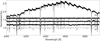 |
Fig. 2 Same as Fig. 1 but for the UVES spectrum of supergiant HD 270123. See text for details. |
| In the text | |
|
Fig. 3 Comparison of the observed LSD profiles with the best-fit asymmetric Gaussian profile models. From top left to bottom right: SK -70 77, HD 268729, SOI 404, and HD 268654 (all were classified as blue supergiants). Blue lines indicate the inferred RVs, while the shaded areas reflect the corresponding 1σ uncertainty intervals. |
| In the text | |
|
Fig. 4 Fourier transforms of synthetic line profiles with positions of the first zero indicated with vertical dotted lines. Left panel: ν sin i parameter is varied from 42 km s−1 (blue) to 90 km s−1 (black) with a step of 6 km s−1 (grey). Middle panel: Linear limb darkening coefficient e is varied from 0.2 (black) to 1.0 (light grey), while ν sin i is kept fixed at 50 km s−1. Right panel: A different contribution of the macroturbulence Θ to the total line broadening is assumed: Θ/v sin i = 0.3, 0.6, 1.2 and 1.8, with ν sin i fixed to 50 km s−1. The inset is a zoom onto the region of the position of the first zero. |
| In the text | |
|
Fig. 5 Results of ν sin i inferences. Left panel: positions of the sample stars in the spectroscopic HR diagram. Individual objects are colour coded according to their ν sin i value inferred from the Fourier method. Right panel: comparison of ν sin iSP with ν sin iFT. The grey line shows the case where ν sin iFT and ν sin iSP are equal, while the blue line is an error-weighted fit to the observed values. |
| In the text | |
|
Fig. 6 Positions of the sample stars in the spectroscopic log(Teff)–log(ℒ/ℒ⊙) HR diagram. The UVES and FEROS samples are shown with black and blue symbols with error bars, respectively. Regions of the parameter space covered by the GSSP, TLUSTY, and CMFGEN models are marked with red, blue, and grey shaded areas, respectively. Non-rotating mesa stellar evolution tracks computed for Ζ = 0.006 are shown with black solid lines and are taken from Burssens et al. (2020). Left panel: full parameter range. Right panel: zoom onto the high-luminosity region where the bulk of the sample is situated. |
| In the text | |
|
Fig. 7 Results of the inference of the macroturbulence parameter Θ. Left panel: stellar positions in the spectroscopic HR diagram colour coded by the inferred value of the macroturbulent velocity parameter Θ. Value of the macroturbulent velocity is an error-weighted average of two epochs. Right panel: distribution of the macroturbulent velocity parameter Θ across the sample. |
| In the text | |
|
Fig. 8 Results of the inference of the tangential component of macro-turbulence. Top panel: Histogram of aT contributions derived from observed profiles of the entire sample with aT = 0.5 as an initial assumption, ν sin i varied within errors of ν sin iFT. Middle panel: Histograms of αT contributions derived from observed profiles of the entire sample with different initial assumptions: 0.25 (yellow), 0.5 (blue), 0.75 (green), and ν sin i left to vary freely. Bottom panel: KDE functions for the same data as in the middle panel. Dashed lines mark initial guesses. The fits demonstrate the results are sensitive to the initial guess. |
| In the text | |
|
Fig. 9 Results of the inference of the tangential component of macro-turbulence. Left panel: comparison of Θ measured with fixed tangential component contribution aT = 0.5 and Θ measured when aT is left to vary freely. Right panel: distribution of tangential component contribution aT over Θ. Colour encodes Teff, while symbol size changes with spectroscopic luminosity. |
| In the text | |
|
Fig. 10 Results of the multivariate linear regression models for Θ. Left panel: comparison between Θ and ν sin i. The colours encode Teff, while the symbol sizes scale with spectroscopic luminosity. The red circles show the predicted Θ value from the best multivariate regression model in Eq. (5) for our LMC sample. The red vertical line in the corner indicates a typical error bar for the predicted Θ values and applies to all three panels. Middle panel: comparison between observed Θ and predictor Teff, where Θ predicted from Eq. (5) is colour coded in red. Right panel: comparison of Θ predicted from Eq. (5) and the measured values of Θ. |
| In the text | |
|
Fig. 11 Comparison of Θ observed in our sample and Θ for the sample treated by Simón-Díaz et al. (2017). Circles show the results for our LMC stars, while triangles are the results from Simón-Díaz et al. (2017) for their sample of Ο and Β stars in the Galaxy. Left panel: comparison between observed Θ and ν sin i with the same colour and symbol scheme for Teff as in Fig. 10. Middle panel: comparison between observed Θ and Teff. Right panel: comparison of histograms and KDE for Θ in our sample (blue) and the one of Simón-Díaz et al. (2017; green). |
| In the text | |
|
Fig. 12 Results of Monte Carlo simulations on synthetic profiles of Mg II (top set of panels) and Si III (bottom set of panels) with artificial noise (left panels: S/N = 250, middle panels: S/N = 150, and right panels: S/N = 100) with 1σ, 2σ, and 3σ confidence ellipses. Correlation coefficients ρ are indicated in the right corner of each panel. v sin i is fixed, while ξ and Θ are optimised. The red crosses mark true parameters of the synthetic profiles. |
| In the text | |
|
Fig. C.1 Results of Monte Carlo simulations on synthetic profiles of Mg II 4481 Å line with artificial noise (left panel: S/N = 250, middle panel: S/N = 150, and right panel: S/N = 100) with 1, 2, and 3σ confidence ellipses. Correlation coefficients ρ are indicated in the right corner of each panel, υ sin i is fixed, while Θ and ξ are optimised. The red crosses mark the true parameters of the synthetic profiles. |
| In the text | |
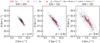 |
Fig. C.2 Same as Fig. C.1 for another set of parameters ν sin i, ξ, and Θ in the synthetic profile. |
| In the text | |
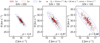 |
Fig. C.3 Same as Fig. C.1 for another set of parameters ν sin i, ξ, and Θ in the synthetic profile. |
| In the text | |
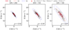 |
Fig. C.4 Same as Fig. C.1 for another set of parameters ν sin i, ξ, and Θ in the synthetic profile. |
| In the text | |
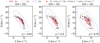 |
Fig. C.5 Same as Fig. C.1 for another set of parameters ν sin i, ξ, and Θ in the synthetic profile. |
| In the text | |
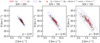 |
Fig. C.6 Same as Fig. C.1 for another set of parameters ν sin i, ξ, and Θ in the synthetic profile. |
| In the text | |
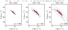 |
Fig. C.7 Same as Fig. C.1 for another set of parameters ν sin i, ξ, and Θ in the synthetic profile. |
| In the text | |
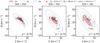 |
Fig. C.8 Same as Fig. C.1 for another set of parameters ν sin i, ξ, and Θ in the synthetic profile. |
| In the text | |
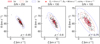 |
Fig. C.9 Same as Fig. C.1 for another set of parameters ν sin i, ξ, and Θ in the synthetic profile. |
| In the text | |
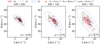 |
Fig. C.10 Same as Fig. C.1 for another set of parameters ν sin i, ξ, and Θ in the synthetic profile. |
| In the text | |
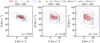 |
Fig. C.11 Same as Fig. C.1 for another set of parameters ν sin i, ξ, and Θ in the synthetic profile. |
| In the text | |
|
Fig. C.12 Same as Fig. C.1 but v sin i is optimised as well as ξ and Θ, resulting in three free parameters. |
| In the text | |
|
Fig. C.13 Same as Fig. C.1 but v sin i and aT are optimised as well as ξ and Θ, resulting in four free parameters. Only the results for S/N=250 are shown. |
| In the text | |
Current usage metrics show cumulative count of Article Views (full-text article views including HTML views, PDF and ePub downloads, according to the available data) and Abstracts Views on Vision4Press platform.
Data correspond to usage on the plateform after 2015. The current usage metrics is available 48-96 hours after online publication and is updated daily on week days.
Initial download of the metrics may take a while.