| Issue |
A&A
Volume 674, June 2023
|
|
|---|---|---|
| Article Number | A228 | |
| Number of page(s) | 12 | |
| Section | Planets and planetary systems | |
| DOI | https://doi.org/10.1051/0004-6361/202346214 | |
| Published online | 27 June 2023 | |
Kinetic simulations of solar wind plasma irregularities crossing the Hermean magnetopause
1
Institute of Space Science,
Măgurele
077125, Romania
e-mail: This email address is being protected from spambots. You need JavaScript enabled to view it.
2
Royal Belgian Institute for Space Aeronomy,
Brussels
1180, Belgium
3
Belgian Solar Terrestrial Center of Excellence,
Brussels, Belgium
Received:
22
February
2023
Accepted:
20
April
2023
Abstract
Context. The physical mechanisms that favor the access of solar wind plasma into the magnetosphere have not been entirely elucidated to date. Studying the transport of finite-sized magnetosheath plasma irregularities across the magnetopause is fundamentally important for characterizing the Hermean environment (of Mercury) as well as for other planetary magnetic and plasma environments.
Aims. We investigate the kinetic effects and their role on the penetration and transport of localized solar wind or magnetosheath plasma irregularities within the Hermean magnetosphere under the northward orientation of the interplanetary magnetic field.
Methods. We used three-dimensional (3D) particle-in-cell (PIC) simulations adapted to the interaction between plasma elements (irregularities or jets) of a finite spatial extent and the typical magnetic field of Mercury’s magnetosphere.
Results. Our simulations reveal the transport of solar wind plasma across the Hermean magnetopause and entry inside the magnetosphere. The 3D plasma elements are braked and deflected in the equatorial plane. The entry process is controlled by the magnetic field gradient at the magnetopause. For reduced jumps of the magnetic field (i.e., for larger values of the interplanetary magnetic field), the magnetospheric penetration is enhanced. The equatorial dynamics of the plasma element is characterized by a dawn-dusk asymmetry generated by first-order guiding center drift effects. More plasma penetrates into the dusk flank and advances deeper inside the magnetosphere than in the dawn flank.
Conclusions. The simulated solar wind or magnetosheath plasma jets can cross the Hermean magnetopause and enter into the magnetosphere, as described by the impulsive penetration mechanism.
Key words: plasmas / magnetic fields / planet–star interactions / methods: numerical
© The Authors 2023
 Open Access article, published by EDP Sciences, under the terms of the Creative Commons Attribution License (https://creativecommons.org/licenses/by/4.0), which permits unrestricted use, distribution, and reproduction in any medium, provided the original work is properly cited.
This article is published in open access under the Subscribe to Open model. This email address is being protected from spambots. You need JavaScript enabled to view it. to support open access publication.
1 Introduction
The Earth’s magnetopause is frequently impacted by finite-sized plasma irregularities of solar wind or magnetosheath origins that generate various effects on the geomagnetic environment (e.g., Lemaire & Roth 1978; Plaschke et al. 2016). These plasma irregularities are known in the scientific literature under various names, for instance, as filamentary plasma elements (Lemaire 1977; Lundin & Aparicio 1982; Lyatsky et al. 2016a), plas-moids (Lemaire 1985; Echim & Lemaire 2000; Gunell et al. 2014; Karlsson et al. 2015; Goncharov et al. 2020), transient flux enhancements (Němeček et al. 1998), high-kinetic energy density jets (Amata et al. 2011), super-fast plasma streams (Savin et al. 2012), localized density enhancements (Karlsson et al. 2012), dynamic pressure enhancements (Archer & Horbury 2013), or high-speed magnetosheath jets (Plaschke et al. 2013; Wing et al. 2014; Vuorinen et al. 2019; Escoubet et al. 2020; Raptis et al. 2020; Dmitriev et al. 2021). Some of them are able to penetrate the magnetopause and have been observed deep inside the magnetosphere (Lundin & Aparicio 1982; Lundin et al. 2003; Gunell et al. 2012; Shi et al. 2013; Dmitriev & Suvorova 2015; Lyatsky et al. 2016a,b). For instance, Lundin et al. (2003) and Gunell et al. (2012) used Cluster data to study the penetration of solar wind plasma clouds and magnetosheath plasmoids through the dayside magnetopause. These authors conclude that the transport process inside the magnetosphere exhibit similarities with the impulsive penetration mechanism proposed by Lemaire & Roth (1978) to explain such phenomena. Dmitriev & Suvorova (2015) performed a statistical analysis of the jets detected by THEMIS in the magnetosheath and showed that more than 60% of them do penetrate across the magnetopause and do have, overall, electrodynamic properties consistent with the impulsive penetration mechanism. The investigations of Lyatsky et al. (2016a,b) based on Cluster observations emphasize the stable antisunward motion of the magnetosheath filaments inside the magnetosphere, suggesting their detachment from the magne-tosheath background and penetration inside the magnetosphere.
The transport of finite-sized plasma irregularities across magnetic discontinuities, as the magnetopause, is a key process not only for the geomagnetic environment, but also for other planetary plasma environments. Recently, Karlsson et al. (2016, 2021) used MESSENGER data to study the small-scale plasma structures in Mercury’s magnetosheath. Their investigation revealed a relatively large number of localized magnetic structures in the Hermean magnetosheath (of Mercury) and nearby solar wind with similar properties to the high-speed plasma jets identified in the Earth’s magnetosheath. Unfortunately, due to some limitations in the plasma measurements on board MESSENGER, this study does not provide the density and bulk velocity of the observed structures, but only their magnetic signatures. The BepiColombo mission around Mercury will provide a great opportunity to continue this kind of investigation.
The interaction of localized plasma structures with nonuniform magnetic fields was simulated in the past using both fluid and kinetic approaches. There are several magnetohydro-dynamic and hybrid simulations performed in a magnetospheric context as, for instance, Ma et al. (1991), Savoini et al. (1994), Dai & Woodward (1994, 1995, 1998), Huba (1996). The physics treated by these simulations is truncated since important physical processes occurring at kinetic scales, such as the self-polarization electric field, are disregarded (see Echim & Lemaire 2000 for a review). More recently, Palmroth et al. (2018, 2021) used two-dimensional (2D) hybrid-Vlasov simulations to investigate the formation and properties of high-speed plasma jets in the Earth’s magnetosheath. It has been shown that the simulated jets exhibit similar features with the ones detected in-situ in the magnetosheath. Similarly, Preisser et al. (2020) proposed various generation mechanisms of localized jets or plasmoids based on 2D hybrid simulations. All the cited papers are focused on jets formation or properties and did not discuss their interaction with the magnetopause and the subsequent evolution. In the Hermean environment, Fatemi et al. (2020) used the AMITIS code (Fatemi et al. 2017) to run three-dimensional (3D) hybrid simulations for the precipitation of solar wind protons onto the surface of planet Mercury under various solar wind conditions, but did not considered the problem of plasma jets.
The fully kinetic simulations performed on the topic of finite-sized plasma irregularities interaction with magnetic barriers (e.g., Galvez 1987; Galvez et al. 1988; Livesey & Pritchett 1989; Galvez & Borovsky 1991; Cai & Buneman 1992; Neubert et al. 1992; Hurtig et al. 2003; Gunell et al. 2009) are limited to magnetic configurations that are either uniform or very specific for certain laboratory experiments, thus only partially relevant for the interaction of high-speed plasma jets with planetary magnetospheres. Karimabadi et al. (2014) considered 2D fully kinetic and hybrid approaches to simulate the solar wind interaction with the terrestrial magnetosphere. It has been argued that the foreshock turbulence gives rise to high-speed plasma jets that further move inside the magnetosheath. Some of the simulated jets reach the magnetopause, but are not traced further.
Voitcu & Echim (2016, 2017) used 3D particle-in-cell (PIC) simulations to emphasize the electric self-polarization of finite-sized plasma irregularities or jets streaming across transverse magnetic discontinuities. It has been shown that the plasma-field interaction process is controlled by the height of the magnetic barrier and the initial momentum of the plasma jets, separating them into penetrating and non-penetrating ones. While the penetrating jets are braked when the magnetic field increases, the non-penetrating ones are split into two counter-streaming flows drifting tangentially to the magnetic discontinuity surface. Their kinetic structure revealed the presence of crescent-shaped velocity distributions after the interaction with the magnetic discontinuity (Voitcu & Echim 2018). More recently, Lavorenti et al. (2022) considered an implicit particle-in-cell code (iPIC3D – Markidis et al. 2010) to globally simulate the magnetosphere of planet Mercury. These authors focused on the self-consistent formation and characterization of the magnetosphere under different orientations of the interplanetary magnetic field (IMF), but did not envisage the problem of high-speed plasma jets interacting with the magnetopause.
In this paper, we used 3D PIC simulations and theoretical modeling to study the kinetic effects associated with the interaction between finite-sized solar wind or magnetosheath plasma structures and the dayside region of the Hermean magnetosphere under a northward orientation of the interplanetary magnetic field. We focus on the equatorial dynamics and asymmetric evolution of the plasma structures penetrating inside the magne-tospheric cavity. Thus, we extend our previous PIC simulations on the topic of plasma-field interaction near magnetic discontinuities (Voitcu & Echim 2016, 2017, 2018) by considering a simulation setup which corresponds to the magnetosphere of planet Mercury. While the aforementioned simulations were “local,” here we discuss a more “global” approach that is specific to a small magnetospheric system. We provide new physical insight on the transport mechanisms of penetrating plasma inside the Hermean magnetosphere. The simulation results are discussed in the context of the impulsive penetration mechanism (Lemaire 1985).
This paper is organized as follows. In the second section, we describe the setup of our simulations. In the third section, we present the results obtained, while in the last section, we give our conclusions.
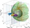 |
Fig. 1 Simulation setup for cases A (frontal injection), B (dawn flank injection), and C (dusk flank injection) in the MSM reference frame. The Hermean magnetopause is drawn in green according to Shue’s model (Shue et al. 1997). The KT17 magnetic field lines (Korth et al. 2017) are represented in red, while the northward magnetic field lines outside Mercury’s magnetosphere are shown in blue. We illustrate with colored boxes the injection regions corresponding to the three simulated plasma structures: Yellow for case A, blue for case B, and purple for case C. The initial plasma bulk velocity is shown with black arrows. |
2 Simulation setup
The simulation setup illustrated in Fig. 1 is adapted for the interaction between 3D plasma structures originating from the solar wind or magnetosheath and the dayside magnetosphere of planet Mercury. Since our goal is to investigate the local microphysics of the interaction process in the vicinity of the Hermean magnetopause, we assume that the global magnetospheric configuration is established prior to the interaction of the finite-sized plasma structures with the magnetosphere. Thus, the global simulation of the Hermean magnetosphere formation is beyond the scope of our paper. The simulated magnetic field has two components, namely, (i) the background (or external) magnetic field and (ii) the internal magnetic field produced by the localized plasma element itself. The background magnetic field is steady-state and is added at each time-step to the self-consistent field computed during the simulation runtime. It also has two components corresponding to (i) the magnetospheric field of Mercury and (ii) the solar wind. The transition between these two components of the magnetic field is imposed along a 3D surface defined by Shue’s model of the magnetopause (Shue et al. 1997). Thus, for a given position (x, y, z) within the simulation domain, the background magnetic field is:
 (1)
(1)
where: BMSP is the magnetospheric field of planet Mercury provided by the KT17 model (Korth et al. 2017), BIMF is the interplanetary magnetic field which is assumed to be uniform, r is the radial distance from Mercury’s dipole to the (x,y, z) point, and rMP is the radial distance to the 3D magnetopause surface.
The background plasma is disregarded in the present work and the finite-sized plasma element is streaming in a vacuum towards the magnetopause, similarly to a high-speed plasma jet characterized by an excess of dynamic pressure in a tenuous background environment (e.g., Karlsson et al. 2012). The presence of a background plasma directly impacts the parallel and perpendicular dynamics of the high-speed plasma jets, as discussed, for instance, by Borovsky (1987). The laboratory experiments performed by Wessel et al. (1988) have shown that the background plasma can reduce the self-polarization electric field and cross-field propagation, but only for background densities equal to or larger than the plasmoid density. Thus, for high-speed plasma jets characterized by an excess of density with respect to the background plasma, as the ones observed in the magnetosheath, the cross-field propagation is possible. We plan to include a background plasma in our future simulations.
The electrons and protons of the finite-sized plasma element are uniformly distributed over a 3D region outside the magnetosphere at t = 0. The injection area is localized close to the subsolar magnetopause in case A (frontal injection) and in the two magnetospheric flanks in cases B (dawn flank injection) and C (dusk flank injection). Their initial velocities are generated according to a displaced Maxwellian with the average velocity pointing along the negative XMSM direction, where MSM denotes the Mercury solar magnetospheric coordinate system. The two species have identical densities and temperatures at t = 0. The IMF direction is northward, while the initial self-consistent electric and magnetic fields are set to 0 in the entire simulation domain. There is no external electric field.
The plasma-beta parameter is small (β = 0.01) and the plasma dielectric constant is large (ɛ = 190); ɛ = 1 + (ωpi/ωLi)2, where ωpi and ωLi are the ion Langmuir and Larmor frequencies (e.g., Chen 1984). For large values of e, the self-polarization electric field plays an important role for the propagation of the plasma element across the magnetic field (e.g., Schmidt 1960; Lemaire 1985; Echim & Lemaire 2005; Voitcu & Echim 2016). The perpendicular size of the plasma element with respect to the IMF direction, L⊥, is 13 times larger than the thermal ion Larmor radius, that is, equal to 0.76 Mercury radii. These values are consistent with the scale sizes determined by Karlsson et al. (2021) for the localized magnetic structures identified by MESSENGER in Mercury’s magnetosheath and the nearby solar wind. Thus, we simulate small Larmor radius plasma clouds that are large with respect to the Hermean magnetospheric cavity.
Our simulation code embraces a similar approach to the one employed by Buneman (1993) in TRISTAN. The PIC model is explicit, electromagnetic, and relativistic. The geometry is 3D in the configuration space and velocity space. The boundaries of the simulation domain are periodic and kept as far as possible from the localized plasma element. Currently, there are no inner boundary conditions for the planetary surface. To quantify the amount of plasma crossing Mercury’s surface at a given time, we define the planetary penetration degree: ΓP(t) = MIN(t)/M0, where MIN is the total mass of plasma reaching the surface of Mercury at a time, t, while M0 is the initial mass of the plasma element. Since the charged particles are injected from the solar wind, ΓP(0) = 0. In order to avoid the unrealistic accumulation of plasma inside the planet, the simulation is stopped when the planetary penetration degree reaches a certain critical threshold, namely, ΓP = 4%.
The list of input parameters used in cases A, B, and C is given in Table 1. The center of the plasma element at t = 0 is localized in (X0, Y0, Z0) in the MSM reference system. All three plasma elements are injected from the equatorial plane, that is, Z0 = 0. In case A, Y0 = 0 (frontal injection), while in cases B and C, Y0 = ∓0.76 RM (injection from flanks). The total number of simulated particles is 20 million per species, while the number of particles per simulation grid-cell at initialization is 100 per species. The proton-to-electron mass ratio is 36. For the KT17 model, we used the following input parameters: rh = 0.39 AU and DI = 50, where rh is Mercury’s heliocentric distance expressed in astronomical units and DI the magnetic disturbance index (Anderson et al. 2013). The subsolar magnetopause distance used in Shue’s model is Rss = (2.06873 – 0.00279 · DI) •  (Korth et al. 2017), while the magnetotail flaring level is α = 0.5.
The physical quantities are normalized as follows throughout the paper: the number density to the initial value, n0, the charge density to ρ0 = en0 (where e is the elementary charge), the bulk velocity to the injection value, U0, the magnetic field induction to the IMF value, B0, the electric field intensity to E0 = U0B0 and the spatial coordinates to Mercury’s radius, RM.
Input parameters
3 Numerical results
In the first simulated case, the plasma element is injected upstream the subsolar magnetopause: ΔR = 2.6 rLi = 0.15 RM, where ΔR is the distance between the propagation front of the plasma element at t = 0 and the magnetopause nose located at Rss = 1.41 RM. The background magnetic field increases by 81% across the model magnetopause, from B0 in the solar wind and magnetosheath to Bss just inside the magnetosphere. The simulation is stopped at ωLit = 10 when ΓP = 4%; ωLi is the ion Larmor frequency outside the magnetosphere. The plasma bulk velocity is computed from the average velocities of the electrons and ions: U = (ρmeUe + ρmiUi)/(ρme + ρmi), where ρme and ρmi are the mass densities of the two plasma species. Note: the bulk velocity is calculated only for those grid-cells with particle densities higher than 8% of n0 in order to avoid unrealistically large velocities in the less populated bins. This high-density core of the plasma element is illustrated with a white or blue contour in various plots throughout the paper.
The key element that sustains the transport of finite-sized plasma structures across magnetic barriers, such as the magnetopause, is the self-polarization electric field (e.g., Schmidt 1960; Borovsky 1987). When a plasma element of finite spatial extent is injected into a transverse magnetic field, the charge-dependent Lorentz force deflects the electrons and ions in opposite directions and two space charge layers of reversed polarity are formed at its lateral edges across the perpendicular direction to both the magnetic field and plasma bulk velocity. As long as ɛ ≫ 1, these layers maintain a polarization electric field inside the quasineutral bulk of plasma that further sustains its cross-field propagation: E0 = B0 × U0.
In Fig. 2, we illustrate the self-polarization kinetic effect for case A, shortly after injection (ωLit = 0.6) and prior to the interaction with the non-uniform magnetic field. The top and middle panels show the total charge density (ρ = ρe + ρi) and self-consistent electric field in the XMSM = 1.96 RM cross-section localized outside the magnetosphere. The electric field is drawn with vectors and its Ey component is color-coded. Large purple arrows are used to indicate the background magnetic field orientation. The bottom panel illustrates the variation profiles of ρ(y) and Ey (y) averaged along the magnetic field direction from ZMSM = −0.11 RM to ZMSM = +0.11 RM. This interval corresponds to the bulk region of plasma bounded by the white contour in the top and middle panels. The horizontal yellow line marks the value of Ey = −E0. We can easily notice that the lateral edges of the plasma element are electrically polarized. Indeed, a negative space charge layer is observed around YMSM ≈ −0.37 RM, while a positive one is evidenced around YMSM ≈ +0.40 RM. They are illustrated with tall magenta boxes in Fig. 2. In the region between these two layers, the plasma is quasineutral (ρ ≈ 0) and the electric field intensity is Ey ≈ –U0B0. This self-polarization electric field drives the plasma element across the transverse magnetic field.
In the top panel of Fig. 3, we illustrate the electron number density at the end of run, while in the middle panel, the Ux component of the plasma bulk velocity, both for the meridional cross-section YMSM = 0. The plasma element injected from the solar wind is able to penetrate inside the Hermean magnetosphere. Indeed, as can be noticed in Fig. 3, almost the entire plasma structure is located downstream the Shue’s magnetopause at the end of run. The magnetospheric entry is accompanied by the strong braking of the plasma element while streaming into the increasingly larger magnetic field. The bulk velocity is reduced from U0, prior to the interaction with the magnetopause, to Ux ≈ 0, at the propagation front in ZMSM = 0. Simultaneously, the penetrating plasma is expanding along the magnetic field lines towards the planetary surface at high latitudes. The electron density in the top panel of Fig. 3 is characterized by wave structures that can also be observed in later figures. Wave phenomena in plasmoids penetrating across magnetic barriers have been emphasized in the past with numerical simulations (e.g., Gunell et al. 2008, 2009), satellite measurements (e.g., Gunell et al. 2014) and laboratory experiments (e.g., Hurtig et al. 2004). The study of waves is beyond the scope of our paper, but we shall approach these phenomena in a future publication.
In order to quantify the entry process, we defined the magnetospheric penetration degree:  , where
  is the total mass of plasma penetrating inside the magnetosphere at time t (i.e., downstream the magnetopause). Since the charged particles are injected from the solar wind, ΓMSP(0) = 0. The blue curve in the bottom panel of Fig. 3 shows the time evolution of ΓMSP for case A. By the end of run, 72% of the initial mass of plasma injected from the solar wind crossed the magnetopause surface and entered inside the magnetosphere. This ratio is higher when the magnetic jump at the magnetopause is reduced. Indeed, by running a supplemental simulation with Bss/B0 = 1.29, we obtained a magnetospheric penetration degree of 81% at ωLit = 10 (the red curve in Fig. 3). We note that the plasma dielectric constant was kept unchanged in the new simulation run in order to maintain the same level of electric self-polarization. Thus, by reducing the height of the magnetic barrier, Bss – B0, by 50%, the amount of plasma crossing the magnetopause increases by
  , where an upper index of 1 refers to Bss/B0 = 1.81 and an upper index of 2 to Bss/B0 = 1.29.
The dynamics of the plasma element in the equatorial plane (ZMSM = 0) is emphasized in Fig. 4, where we illustrate the electron and ion densities (top panels), perpendicular bulk velocity components (middle panels), and perpendicular electric field components (bottom panels) at the end of run (ωLit = 10). We note that the plasma element is deflected along both the positive and negative directions of the YMSM axis as it enters inside the magnetosphere. Indeed, Uy > 0 for the plasma regions having YMSM > 0 and, oppositely, Uy < 0 for YMSM < 0. At the furthermost areas of the plasma element along YMSM, we have |Uy| ≈ U0/2. This deflection process is sustained by the Ex component of the electric field which is negative for YMSM > 0 and positive for YMSM < 0. On the other hand, Ux < 0 for YMSM > 0 and Ux ≈ 0 for YMSM < 0, consistent with the sign of Ey. Thus, the duskward wing of the deflected plasma element is streaming faster along -XMSM with respect to the dawnward wing which is virtually stopped, leading to an asymmetric evolution inside the magnetosphere.
To better visualize the equatorial dynamics of the penetrating plasma element, the orientation and magnitude of the perpendicular plasma bulk velocity are shown in the top panels of Fig. 5. In the bottom panels, we plot the orientation and magnitude of the zero-order (or electric) drift velocity, UE = E × B/B2, computed with the self-consistent electric field (illustrated in the bottom panels of Fig. 4) and the background magnetic field illustrated with the greenish color map (since β ≪ 1, we neglected the self-consistent magnetic field). By comparing the top and bottom panels of Fig. 5, we can notice that the penetrating plasma is drifting with U⊥ ≈ UE inside the magnetosphere and the YMSM deflection is not totally symmetrical. The perpendicular bulk velocity is a bit larger in the dusk flank (YMSM > 0) than in the dawn flank (YMSM < 0). This dawn-dusk asymmetry in the equatorial plane can be observed also in the top panels of Fig. 4. Indeed, the particle density is larger in the dusk flank with respect to the dawn flank for both plasma species.
The asymmetry is emphasized more clearly in Fig. 6 where we illustrate ion density isosurfaces at the beginning (yellow) and the end of run (purple). The top and middle panels show the 3D simulation box observed from the Sun (top) and from above the north pole (middle). The isosurfaces are drawn for ni/n0 = 0.33 at t = 0 and ni/n0 = 0.13 at ωLit = 10. While the plasma element or jet is symmetric at injection, its shape changes asymmetrically while moving into the magnetosphere. There is a displacement of the entire plasma element along the +YMSM direction. To quantify this asymmetry, we compare the time evolution of the plasma penetration degree computed for the two magnetospheric flanks:  for the dawn flank and
  for the dusk flank;
  is the total mass of plasma penetrating inside the dawn flank of the Hermean magnetosphere (i.e., downstream the magnetopause for YMSM < 0) at time, t, while
  corresponds to the mass of plasma penetrating inside the dusk flank (i.e., downstream the magnetopause for YMSM > 0). The results obtained are shown in the bottom panel of Fig. 6. While in the early stages of the simulation, we have
  , later on, as the plasma element advances inside the magnetosphere, the penetration degree in the dusk flank exceeds the one in the dawn flank. By the end of run,
  and
and  . Thus, the amount of solar wind plasma crossing the magnetopause into the dusk flank is larger than the one corresponding to the dawn flank by
  .
.
The impulsive penetration mechanism proposed by Lemaire (1977, 1985) and Lemaire & Roth (1978) embraces a self-consistent kinetic model that couples the first-order guiding center approximation with Ampère’s law to explain the entry and transport of solar wind plasma elements inside the magnetosphere. According to this model, the perpendicular bulk velocity of the finite-sized plasma elements is given by the superposition between the zero-order drift velocity corresponding to the self-polarization electric field and a first-order term corresponding to the gradient-B and curvature drift velocities of the electrons averaged over their corresponding velocity distribution function. The zero-order drift velocity satisfies the following equation for a non-uniform magnetic field (Lemaire 1985):
 (2)
(2)
while the first-order drift velocity, U1, is given by (Lemaire 1985):
 (3)
(3)
where T⊥α and T||α are the perpendicular and parallel temperatures of species α with masses mα; also, k is Boltzmann’s constant and e is the elementary charge.
We checked if the plasma jet dynamics in our PIC simulations is well described by Eqs. (2) and (3). First, we calculated the zero-order drift velocity that satisfies Eq. (2). For this purpose, we expanded the total time derivative of the zero-order drift velocity in Eq. (2) to obtain a partial differential equation that is further solved with the method of characteristics (e.g., Jeffrey & Dai 2008). The characteristic curves, {X(t), Y(t), Z(t)}, and the solution of Eq. (2) along them, {UE,x(t), UE,y(t), UE,z(t)}, are computed numerically for various sets of initial conditions given at t = 0. We used central finite-differences to discretize the derivatives in Eq. (2).
The initial velocity distribution functions of the simulated electrons and ions are displaced Maxwellians with equal temperatures: T⊥e0 = T⊥i0 = T||e0 = T||i0 = T0. Since the magnetic moment is a constant of motion for both plasma species, the perpendicular temperature increases linearly with the magnetic field magnitude increase: T⊥e = T⊥i = T⊥ = T0B/B0. On the other hand, for simplicity, we consider the parallel temperature unchanged: T||e = T||i = T|| = T0. This constraining condition could be further relaxed to a more general situation with T|| = T||(x, y, z), but such an extension is beyond the scope of our current study.
We traced the characteristic curves of Eq. (2) for three different sets of initial conditions that sample the center (Y2 = Y0) of the plasma element and its lateral edges (Y1 = Y0 – L⊥/2 and Y3 = Y0 + L⊥/2) along the B0 × U0 direction. Thus, we provided the following initialization upstream the magnetopause: {X0, Y1, Z0, U0, 0,0} for the first curve, {X0, Y2, Z0, U0, 0,0} for the second curve, and {X0, Y3, Z0, U0, 0, 0} for the third curve. The integration time is ωLit = 10. The results obtained are shown in the top panel of Fig. 7. We superposed the three characteristics curves (integrated from t = 0 to ωLit = 10) onto the PIC solution illustrated in the bottom-left panel of Fig. 5 (at ωLit = 10). The characteristic curves are color coded with the magnitude of the zero-order drift velocity that satisfies Eq. (2).
Since the magnetic transition at the simulated magnetopause is very sharp, the guiding center approximation and, consequently, the impulsive penetration model are not valid at the interface between the solar wind and the simulated Hermean magnetosphere. We note that this is just a limitation of this particular simulation and the real thickness of the magnetopause is on the order of several ion Larmor radii (e.g. Roth et al. 1996; Haaland et al. 2004; Dibraccio et al. 2013). In order to surpass this limitation, we considered a supplementary class of initial conditions for the three characteristic curves, provided just downstream the magnetopause. They are extracted from the PIC simulation shortly after the propagation front of the plasma element crosses the magnetopause, namely, at ωLit = 2. We note that the PIC solution is independent on the validity of the guiding center approximation. Here, we have the initialization downstream the magnetopause: { , Y1, Z0,
  , −0.12U0,0} for the first curve, {
 , Y2, Z0,
  , 0,0} for the second curve, and {
 , Y3, Z0,
  , +0.12U0, 0} for the third curve, where
  and
and  . The integration time covers the interval from ωLit = 2 to ωLit = 10. The results obtained are shown in the bottom panel of Fig. 7. As expected, the theoretical solution computed for the downstream initialization matches the PIC simulation significantly better than the theoretical solution computed for the upstream initialization. We shall impose a smoother transition of the magnetic field at the magnetopause in our future simulations.
It can be easily noticed that the two lateral characteristic curves are deflected symmetrically inside the magnetospheric cavity, while the central one remains unperturbed. Indeed, the curve initialized in Y1 < 0 is pushed dawnward, while the one initialized in Y3 > 0 is pushed duskward. On the other hand, the zero-order drift velocity is significantly reduced for larger values of the magnetic field. For the central characteristic curve initialized in Y2 = 0, the zero-order drift velocity at ωLit = 10 is UE,x = –0.20 U0 for the upstream initialization and UE,x = +0.16 U0 for the downstream initialization. Thus, the forward motion is strongly slowed down and even stopped and reversed towards the +XMSM axis. This behavior is also observed in our PIC simulations. Indeed, the bulk velocity at the propagation front of the plasma element near the equatorial plane is slightly positive, Ux ≈ +0.10 U0, as can be seen in Figs. 3 and 4.
The dominant symmetrical deflection of the plasma element in the equatorial plane is generated through the zero-order drift velocity. However, the PIC simulations also show a displacement of the entire plasma structure along the +YMSM direction. To address this behavior, we investigated the first-order drift velocity given by Eq. (3). Using the assumptions on the temperature variation considered for solving Eq. (2), we computed the spatial distribution of U1. The results obtained are shown in Fig. 8 for the total first-order drift velocity field and its gradient-B and curvature terms.
We can notice that the U1x component of the first-order drift velocity is positive in the dawn flank and negative in the dusk flank. On the other hand, the U1y component is always positive. The magnitude, U1, increases as we advance inside the magnetosphere and is larger in the front than in the flanks (for a fixed XMSM value). At the propagation front of the simulated plasma element, we have U1 = 0.02 U0 in YMSM = 0 and U1 = 0.025 U0 in YMSM = 0.63 RM. With respect to the local value of the plasma bulk velocity, U1 ≈ 0.50 U⊥ around YMSM = 0 and decreases to U1 ≈ 0.05 U⊥ around YMSM = 0.63 RM. The ratio between the gradient-B and curvature terms in Eq. (3) is ![Mathematical equation: ${{U_1^{\nabla B}} \mathord{\left/ {\vphantom {{U_1^{\nabla B}} {U_1^{cr\upsilon }\, \in \,\left[ { \sim 1.2, \sim 2.6} \right]}}} \right. \kern-\nulldelimiterspace} {U_1^{cr\upsilon }\, \in \,\left[ { \sim 1.2, \sim 2.6} \right]}} $](/articles/aa/full_html/2023/06/aa46214-23/aa46214-23-eq24.png) , with an average value of ~1.8. This ratio decreases for larger parallel temperatures.
, with an average value of ~1.8. This ratio decreases for larger parallel temperatures.
Figure 9 shows the variation of |Y(t)| for the two lateral characteristic curves initialized in the dawn (|YDa(t)|, solid lines) and dusk (|YDu(t)|, dashed lines) flanks of the magnetosphere. The top and bottom panels correspond to the theoretical solution computed for the upstream and downstream initial conditions, respectively. The total time derivative of UE in Eq. (2) is expanded by considering the following two approaches: (i) with V = UE (blue lines), as in Fig. 7, and (ii) with V = UE + U1 (red lines), where V = (dX/dt, dY/dt, dZ/dt). In this way, we can directly estimate the quantitative impact of the first-order drift velocity on the dawn-dusk deflection of plasma. As can be noticed in both panels of Fig. 9, the ±YMSM displacement of the two characteristic curves is symmetrical (Δ|Y(t)| = |YDu(t)| – |YDa(t)| = 0) when we neglect the first-order term given by Eq. (3). On the other hand, the ±YMSM displacement is clearly asymmetric when the first-order drift velocity is included in the theoretical solution. Indeed, Δ|Y| increases inside the magnetosphere up to 0.09 RM for the upstream initialization and 0.03 RM for the downstream initialization. The duskward (dawn-ward) advance of the dusk (dawn) curve is larger (smaller) than the one corresponding to the symmetrical displacement, leading to the dawn-dusk asymmetric evolution of the plasma element streaming inside the magnetosphere.
The first-order drift velocity given by Eq. (3) is characterized by a dawn-dusk component in both magnetospheric flanks. This first-order term pushes the plasma towards the positive YMSM axis and further leads to an enhanced accumulation of particles in the dusk flank, as shown in Fig. 6. It also generates the asymmetry observed in the XMSM component of the plasma bulk velocity illustrated in Fig. 4. Indeed, while UE,x < 0 in both flanks, the distribution of U1x is antiparallel (U1x ≷ 0 for YMSM ≶ 0) and, consequently, enlarges the antisunward component of the plasma bulk velocity in the dusk flank with respect to the dawn flank, leading to the observed asymmetry. To better emphasize this effect, we performed two supplemental simulations with plasma elements injected from the two magnetospheric flanks.
The results obtained are shown in Fig. 10 for both cases B (dawn flank injection – blue box in Fig. 1) and C (dusk flank injection – purple box in Fig. 1). The minimum distance between the initial propagation front of the plasma elements and the local magnetopause surface is identical to the one used in case A, namely, ΔR = 2.6 rLi = 0.15 RM. At the local magnetopause, in YMSM = ±0.76 RM, the background magnetic field increases by 62% with respect to the solar wind value. The simulation is stopped at ωLit = 11 when the planetary penetration degree is still small, namely, 4% in case B and 3% in case C.
We illustrate in Fig. 10 the electron number density (left panels) and the perpendicular plasma bulk velocity (right panels) in the cross-section ZMSM = 0. Various dynamical properties of the two plasma elements are listed in Table 2. The equatorial evolution of the two simulated plasmas is different, as can be seen in both density and velocity color maps of Fig. 10. Indeed, the dusk flank injection is accompanied by a deeper penetration, while the dawn flank injection is less efficient. The total magnetospheric penetration degree at the end of run (ωLit = 11) is 60% in case B and 70% in case C. Thus, the amount of plasma crossing the magnetopause surface is 17% larger in the dusk flank with respect to the dawn flank. On the other hand, as in case A, the magnetospheric entry is accompanied by the braking of plasma while streaming into the larger magnetic field. The deceleration is different in the two cases. The perpendicular bulk velocity at the propagation front of the plasma element is 14% larger for the dusk flank injection, where U⊥ = 0.89 U0. On the other hand, at the trailing edge, U⊥ ≈ 0 in both cases. The  component of the bulk velocity at the propagation front is almost two times larger for the dusk flank injection, leading to a deeper penetration of plasma inside the magnetosphere, down to 0.63 RM in case C versus 0.89 RM in case B. The magnitude of the first-order drift velocity with respect to the local value of the total plasma bulk velocity varies from 2% (at the propagation front) to 75% (at the trailing edge), as listed in Table 2. Thus, the penetrating plasma is pushed and braked asymmetrically inside the magnetosphere along the YMSM axis by first-order drift effects.
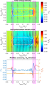 |
Fig. 2 Self-polarization of the plasma element shortly after injection (ωLit = 0.6, where ωLi is the ion Larmor frequency outside the magnetosphere) in the XMSM = 1.96 RM cross-section inside the simulation domain for case A: (top) total charge density and (middle) self-consistent electric field illustrated with vectors (the Ey component is color coded). The profiles of the charge density (blue) and Ey electric field (red) across YMSM (bottom). These profiles are averaged along the ZMSM direction parallel to the magnetic field (shown with large purple arrows in the top and middle panels) from −0.11 RM to +0.11 RM. The white contour in the top and middle panels encloses the high-density core of the plasma element, while the yellow horizontal line in the bottom panel is drawn at Ey = −U0B0. The tall magenta boxes mark the two space charge layers of opposite polarity formed at the edges of the plasma element. |
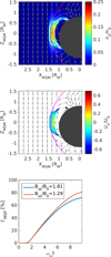 |
Fig. 3 Cross-section YMSM = 0 inside the simulation domain for case A: (top) electron number density and (middle) plasma bulk velocity along the XMSM axis at the end of run (ωLit = 10), where ωLi is the ion Larmor frequency outside the magnetosphere. Both quantities are normalized to their corresponding initial values. The magenta curve illustrates the magnetopause, while the grey arrows indicate the background magnetic field unit vectors. Note: the small overlap of magnetic field vectors in different regions of the simulation domain is just an artifact. The magnetospheric penetration degree variation from initialization to the end of run for Bss/B0 = 1.81 is shown at bottom (blue curve) and Bss/B0 = 1.29 (red curve), where Bss is the magnetic field at the sub-solar magnetopause just inside the magnetosphere and B0 the magnetic field outside the magnetosphere. |
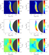 |
Fig. 4 Cross-section ZMSM = 0 inside the simulation domain for case A: (top) electron and ion number densities, (middle) Ux and Uy components of the plasma bulk velocity, and (bottom) Ex and Ey components of the self-consistent electric field, normalized to their corresponding initial values, at the end of run (ωLit = 10). The white contour in the top and bottom panels marks the boundary that separates the higher density bulk of the plasma from its more tenuous regions. The magenta curve is the magnetopause. |
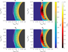 |
Fig. 5 Perpendicular component of the plasma bulk velocity (top) and the zero-order (or electric) drift velocity (bottom) in the ZMSM = 0 cross-section inside the simulation domain for case A, at the end of run (ωLit = 10), illustrated with vectors (left) and color coded (right). The greenish color map shows the magnetic field normalized to its value outside the magnetosphere, while the reddish one the bulk or drift velocity normalized to the injection velocity. The white contour in the left panels encloses the high-density core of the plasma. The magenta curve is the magnetopause. |
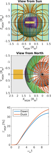 |
Fig. 6 Views of the simulation domain from the Sun (top) and above the north pole (middle) for case A. We show the ion density isosurface at initialization (yellow) and at the end of run (purple). The magneto-spheric penetration degree variation from initialization to the end of run for the dawn (blue curve) and dusk (red curve) flanks (bottom). |
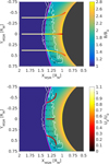 |
Fig. 7 Three characteristic curves of Eq. (2) traced in the equatorial plane (ZMSM = 0). The initial conditions correspond to the central region of the plasma element and its lateral edges. The curves are color coded with the magnitude of the zero-order drift velocity that satisfies Eq. (2) and superposed onto the PIC solution illustrated in the bottom-left panel of Fig. 5. The characteristic curves are computed for two different classes of initial conditions: upstream (top) and downstream (bottom) the magnetopause. |
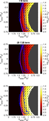 |
Fig. 8 First-order drift velocity given by Eq. (3) in the equatorial plane (ZMSM = 0): (top) gradient-B term, (middle) curvature term, and (bottom) sum of both terms. The orientation of the velocity field is illustrated with unit vectors, while the magnitude is color-coded. The blue contour encloses the high-density core of the simulated plasma element. The magenta curve is the magnetopause. |
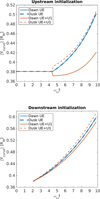 |
Fig. 9 Time evolution of the YMSM coordinate for the two lateral characteristic curves illustrated in Fig. 7: upstream initialization (top) and downstream initialization (bottom). The characteristic curves are calculated with V = UE (blue lines) and V = UE + U1 (red lines). |
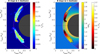 |
Fig. 10 Cross-section ZMSM = 0 inside the simulation domain for cases B (top) and C (bottom) at ωLit = 11: electron number density (left) and perpendicular plasma bulk velocity (right: reddish color map and black unit vectors) superposed onto the background magnetic field magnitude (right: greenish color map). All quantities are normalized to their corresponding initial values. |
Magnetospheric penetration and dynamical properties
4 Conclusions
In the present paper, we use 3D PIC simulations to investigate the interaction between solar wind or magnetosheath plasma elements (or irregularities, jets) and the day side Hermean magnetosphere. The finite-sized jets are streaming towards the magnetopause of Mercury for a northward orientation of the interplanetary magnetic field. We focus on the interaction of the plasma elements with the non-uniform magnetospheric field of planet Mercury and disregard the effects of the background plasma. Here are the main findings of our work:
The solar wind plasma elements are able to cross the magnetopause and penetrate inside the Hermean magnetosphere. The jets’ entry is accompanied by strong braking while streaming into the increasingly larger magnetic field. By reducing the height of the magnetic barrier, the amount of solar wind plasma crossing the magnetopause surface increases.
The plasma elements are deflected in the equatorial plane along both positive and negative directions of the YMSM axis as they enter inside the magnetosphere. The equatorial deflection is asymmetrical. The amount of solar wind plasma crossing the magnetopause surface into the dusk flank is larger than the one corresponding to the dawn flank. Conversely, the braking of the plasma elements is stronger in the dawn flank. Thus, the solar wind plasma elements interacting with the dusk flank magnetopause are able to penetrate deeper inside the Hermean magnetosphere.
The plasma dynamics revealed by our PIC simulations is consistent with the impulsive penetration mechanism. The self-polarization electric field acting inside the quasineutral bulk of plasma sustains the motion across the transverse magnetic field and further determines its equatorial deflection along the YMSM axis. Although it is symmetrical in the zero-order approximation, the equatorial dynamics is characterized by a dawn-dusk asymmetry generated through first-order drift effects. The duskward deflection of the solar wind plasmoids penetrating impulsively in the magnetosphere has been advocated for the first time by Lemaire (1985) for the terrestrial magnetosphere. This study stands as the first numerical confirmation of this kinetic effect.
The physical mechanism we discuss in this paper can explain the transport of high-speed plasma jets across the frontside magnetopause of the planet Mercury in the context of the northward IMF. The BepiColombo mission provides a great opportunity to search for such kinds of plasma structures using in situ data in the vicinity of the Hermean magnetopause.
Acknowledgements
The authors acknowledge support from the Romanian Ministry of Research, Innovation and Digitalization through projects PN-III-P1-1.1-TE-2019-1288 (SMART), PN-III-P1-1.1-TE-2021-0102 (TWISTER) and National Core Program LAPLAS VII (30N/2023) and also from the European Space Agency through PRODEX project PEA 4000134960 (MISION). Marius Echim acknowledges support from the Belgian Solar-Terrestrial Centre of Excellence (STCE) in Brussels, Belgium.
References
- Amata, E., Savin, S. P., Ambrosino, D., et al. 2011, Planet. Space Sci., 59, 482 [NASA ADS] [CrossRef] [Google Scholar]
- Anderson, B. J., Johnson, C. L., & Korth, H. 2013, Geochem. Geophys. Geosyst., 14, 3875 [NASA ADS] [CrossRef] [Google Scholar]
- Archer, M. O., & Horbury, T. S. 2013, Ann. Geophys., 31, 319 [NASA ADS] [CrossRef] [Google Scholar]
- Borovsky, J. E. 1987, Phys. Fluids, 30, 2518 [NASA ADS] [CrossRef] [Google Scholar]
- Buneman, O. 1993, in Computer Space Plasma Physics: Simulation Techniques and Software, eds. H. Matsumoto, & Y. Omura (Tokyo: Terra Scientific Company) [Google Scholar]
- Cai, D. S., & Buneman, O. 1992, Phys. Fluids B, 4, 1033 [NASA ADS] [CrossRef] [Google Scholar]
- Chen, F. F. 1984, Introduction to Plasma Physics and Controlled Fusion, 2nd edn., Vol. 1: Plasma Physics (New York: Plenum Press) [CrossRef] [Google Scholar]
- Dai, W., & Woodward, P. R. 1994, J. Geophys. Res., 99, 8577 [NASA ADS] [CrossRef] [Google Scholar]
- Dai, W., & Woodward, P. R. 1995, J. Geophys. Res., 100, 14843 [NASA ADS] [CrossRef] [Google Scholar]
- Dai, W., & Woodward, P. R. 1998, J. Plasma Phys., 60, 711 [NASA ADS] [CrossRef] [Google Scholar]
- Dibraccio, G. A., Slavin, J. A., Boardsen, S. A., et al. 2013, J. Geophys. Res. (Space Phys.), 118, 997 [NASA ADS] [CrossRef] [Google Scholar]
- Dmitriev, A. V., & Suvorova, A. V. 2015, J. Geophys. Res. (Space Phys.), 120, 4423 [NASA ADS] [CrossRef] [Google Scholar]
- Dmitriev, A. V., Lalchand, B., & Ghosh, S. 2021, Universe, 7, 152 [NASA ADS] [CrossRef] [Google Scholar]
- Echim, M. M., & Lemaire, J. F. 2000, Space Sci. Rev., 92, 565 [NASA ADS] [CrossRef] [Google Scholar]
- Echim, M. M., & Lemaire, J. F. 2005, Phys. Rev. E, 72, 036405 [NASA ADS] [CrossRef] [Google Scholar]
- Escoubet, C. P., Hwang, K. J., Toledo-Redondo, S., et al. 2020, Front. Astron. Space Sci., 6, 78 [NASA ADS] [CrossRef] [Google Scholar]
- Fatemi, S., Poppe, A. R., Delory, G. T., & Farrell, W. M. 2017, Journal of Physics Conference Series, 837, 012017 [NASA ADS] [CrossRef] [Google Scholar]
- Fatemi, S., Poppe, A. R., & Barabash, S. 2020, J. Geophys. Res. (Space Phys.), 125, e27706 [NASA ADS] [Google Scholar]
- Galvez, M. 1987, Phys. Fluids, 30, 2729 [NASA ADS] [CrossRef] [Google Scholar]
- Galvez, M., & Borovsky, J. E. 1991, Phys. Fluids B, 3, 1892 [NASA ADS] [CrossRef] [Google Scholar]
- Galvez, M., Gary, S. P., Barnes, C., & Winske, D. 1988, Phys. Fluids, 31, 1554 [NASA ADS] [CrossRef] [Google Scholar]
- Goncharov, O., Gunell, H., Hamrin, M., & Chong, S. 2020, J. Geophys. Res. (Space Phys.), 125, e27667 [NASA ADS] [Google Scholar]
- Gunell, H., Hurtig, T., Nilsson, H., Koepke, M., & Brenning, N. 2008, Plasma Phys. Controlled Fusion, 50, 074013 [NASA ADS] [CrossRef] [Google Scholar]
- Gunell, H., Walker, J. J., Koepke, M. E., et al. 2009, Phys. Plasmas, 16, 112901 [NASA ADS] [CrossRef] [Google Scholar]
- Gunell, H., Nilsson, H., Stenberg, G., et al. 2012, Phys. Plasmas, 19, 072906 [NASA ADS] [CrossRef] [Google Scholar]
- Gunell, H., Stenberg Wieser, G., Mella, M., et al. 2014, Ann. Geophys., 32, 991 [NASA ADS] [CrossRef] [Google Scholar]
- Haaland, S., Sonnerup, B., Dunlop, M., et al. 2004, Ann. Geophys., 22, 1347 [NASA ADS] [CrossRef] [Google Scholar]
- Huba, J. D. 1996, J. Geophys. Res., 101, 24855 [NASA ADS] [CrossRef] [Google Scholar]
- Hurtig, T., Brenning, N., & Raadu, M. A. 2003, Phys. Plasmas, 10, 4291 [NASA ADS] [CrossRef] [Google Scholar]
- Hurtig, T., Brenning, N., & Raadu, M. A. 2004, Phys. Plasmas, 11, L33 [NASA ADS] [CrossRef] [Google Scholar]
- Jeffrey, A., & Dai, H.-H. 2008, Handbook of Mathematical Formulas and Integrals, 4th edn. (USA: Academic Press) [Google Scholar]
- Karimabadi, H., Roytershteyn, V., Vu, H. X., et al. 2014, Phys. Plasmas, 21, 062308 [NASA ADS] [CrossRef] [Google Scholar]
- Karlsson, T., Brenning, N., Nilsson, H., et al. 2012, J. Geophys. Res. (Space Phys.), 117, A03227 [Google Scholar]
- Karlsson, T., Kullen, A., Liljeblad, E., et al. 2015, J. Geophys. Res. (Space Phys.), 120, 7390 [NASA ADS] [CrossRef] [Google Scholar]
- Karlsson, T., Liljeblad, E., Kullen, A., et al. 2016, Planet. Space Sci., 129, 61 [NASA ADS] [CrossRef] [Google Scholar]
- Karlsson, T., Heyner, D., Volwerk, M., et al. 2021, J. Geophys. Res. (Space Phys.), 126, e28961 [NASA ADS] [Google Scholar]
- Korth, H., Johnson, C. L., Philpott, L., Tsyganenko, N. A., & Anderson, B. J. 2017, Geophys. Res. Lett., 44, 10, 147 [CrossRef] [Google Scholar]
- Lavorenti, F., Henri, P., Califano, F., et al. 2022, A & A, 664, A133 [NASA ADS] [CrossRef] [EDP Sciences] [Google Scholar]
- Lemaire, J. 1977, Planet. Space Sci., 25, 887 [NASA ADS] [CrossRef] [Google Scholar]
- Lemaire, J. 1985, J. Plasma Phys., 33, 425 [NASA ADS] [CrossRef] [Google Scholar]
- Lemaire, J., & Roth, M. 1978, J. Atmos. Terrestrial Phys., 40, 331 [NASA ADS] [CrossRef] [Google Scholar]
- Livesey, W. A., & Pritchett, P. L. 1989, Phys. Fluids B, 1, 914 [NASA ADS] [CrossRef] [Google Scholar]
- Lundin, R., & Aparicio, B. 1982, Planet. Space Sci., 30, 81 [NASA ADS] [CrossRef] [Google Scholar]
- Lundin, R., Sauvaud, J. A., Rème, H., et al. 2003, Ann. Geophys., 21, 457 [NASA ADS] [CrossRef] [Google Scholar]
- Lyatsky, W., Pollock, C., Goldstein, M. L., Lyatskaya, S., & Avanov, L. 2016a, J. Geophys. Res. (Space Phys.), 121, 7699 [NASA ADS] [CrossRef] [Google Scholar]
- Lyatsky, W., Pollock, C., Goldstein, M. L., Lyatskaya, S., & Avanov, L. 2016b, J. Geophys. Res. (Space Phys.), 121, 7713 [NASA ADS] [CrossRef] [Google Scholar]
- Ma, Z. W., Hawkins, J. G., & Lee, L. C. 1991, J. Geophys. Res., 96, 15751 [NASA ADS] [CrossRef] [Google Scholar]
- Markidis, S., Lapenta, G., & Rizwan-uddin. 2010, Math. Comput. Simul., 80, 1509 [CrossRef] [Google Scholar]
- Neubert, T., Miller, R. H., Buneman, O., & Nishikawa, K. I. 1992, J. Geophys. Res., 97, 12057 [NASA ADS] [CrossRef] [Google Scholar]
- Nemecek, Z., Šafránková, J., Prech, L., et al. 1998, Geophys. Res. Lett., 25, 1273 [NASA ADS] [CrossRef] [Google Scholar]
- Palmroth, M., Hietala, H., Plaschke, F., et al. 2018, Ann. Geophys., 36, 1171 [NASA ADS] [CrossRef] [Google Scholar]
- Palmroth, M., Raptis, S., Suni, J., et al. 2021, Ann. Geophys., 39, 289 [NASA ADS] [CrossRef] [Google Scholar]
- Plaschke, F., Hietala, H., & Angelopoulos, V. 2013, Ann. Geophys., 31, 1877 [NASA ADS] [CrossRef] [Google Scholar]
- Plaschke, F., Hietala, H., Angelopoulos, V., & Nakamura, R. 2016, J. Geophys, Res. (Space Phys.), 121, 3240 [NASA ADS] [CrossRef] [Google Scholar]
- Preisser, L., Blanco-Cano, X., Kajdic, P., Burgess, D., & Trotta, D. 2020, ApJ, 900, L6 [NASA ADS] [CrossRef] [Google Scholar]
- Raptis, S., Karlsson, T., Plaschke, F., Kullen, A., & Lindqvist, P.-A. 2020, J. Geophys. Res. (Space Phys.), 125, e27754 [NASA ADS] [Google Scholar]
- Roth, M., De Keyser, J., & Kuznetsova, M. M. 1996, Space Sci. Rev., 76, 251 [NASA ADS] [CrossRef] [Google Scholar]
- Savin, S., Amata, E., Zelenyi, L., et al. 2012, Ann. Geophys., 30, 1 [NASA ADS] [CrossRef] [Google Scholar]
- Savoini, P., Scholer, M., & Fujimoto, M. 1994, J. Geophys. Res., 99, 19377 [NASA ADS] [CrossRef] [Google Scholar]
- Schmidt, G. 1960, Phys. Fluids, 3, 961 [NASA ADS] [CrossRef] [Google Scholar]
- Shi, Q. Q., Zong, Q. G., Fu, S. Y., et al. 2013, Nat. Commun., 4, 1466 [NASA ADS] [CrossRef] [Google Scholar]
- Shue, J. H., Chao, J. K., Fu, H. C., et al. 1997, J. Geophys. Res., 102, 9497 [NASA ADS] [CrossRef] [Google Scholar]
- Voitcu, G., & Echim, M. 2016, J. Geophys. Res. (Space Phys.), 121, 4343 [NASA ADS] [CrossRef] [Google Scholar]
- Voitcu, G., & Echim, M. 2017, Geophys. Res. Lett., 44, 5920 [NASA ADS] [CrossRef] [Google Scholar]
- Voitcu, G., & Echim, M. 2018, Ann. Geophys., 36, 1521 [NASA ADS] [CrossRef] [Google Scholar]
- Vuorinen, L., Hietala, H., & Plaschke, F. 2019, Ann. Geophys., 37, 689 [NASA ADS] [CrossRef] [Google Scholar]
- Wessel, F. J., Hong, R., Song, J., et al. 1988, Phys. Fluids, 31, 3778 [NASA ADS] [CrossRef] [Google Scholar]
- Wing, S., Johnson, J. R., Chaston, C. C., et al. 2014, Space Sci. Rev., 184, 33 [NASA ADS] [CrossRef] [Google Scholar]
All Tables
All Figures
|
Fig. 1 Simulation setup for cases A (frontal injection), B (dawn flank injection), and C (dusk flank injection) in the MSM reference frame. The Hermean magnetopause is drawn in green according to Shue’s model (Shue et al. 1997). The KT17 magnetic field lines (Korth et al. 2017) are represented in red, while the northward magnetic field lines outside Mercury’s magnetosphere are shown in blue. We illustrate with colored boxes the injection regions corresponding to the three simulated plasma structures: Yellow for case A, blue for case B, and purple for case C. The initial plasma bulk velocity is shown with black arrows. |
| In the text | |
|
Fig. 2 Self-polarization of the plasma element shortly after injection (ωLit = 0.6, where ωLi is the ion Larmor frequency outside the magnetosphere) in the XMSM = 1.96 RM cross-section inside the simulation domain for case A: (top) total charge density and (middle) self-consistent electric field illustrated with vectors (the Ey component is color coded). The profiles of the charge density (blue) and Ey electric field (red) across YMSM (bottom). These profiles are averaged along the ZMSM direction parallel to the magnetic field (shown with large purple arrows in the top and middle panels) from −0.11 RM to +0.11 RM. The white contour in the top and middle panels encloses the high-density core of the plasma element, while the yellow horizontal line in the bottom panel is drawn at Ey = −U0B0. The tall magenta boxes mark the two space charge layers of opposite polarity formed at the edges of the plasma element. |
| In the text | |
|
Fig. 3 Cross-section YMSM = 0 inside the simulation domain for case A: (top) electron number density and (middle) plasma bulk velocity along the XMSM axis at the end of run (ωLit = 10), where ωLi is the ion Larmor frequency outside the magnetosphere. Both quantities are normalized to their corresponding initial values. The magenta curve illustrates the magnetopause, while the grey arrows indicate the background magnetic field unit vectors. Note: the small overlap of magnetic field vectors in different regions of the simulation domain is just an artifact. The magnetospheric penetration degree variation from initialization to the end of run for Bss/B0 = 1.81 is shown at bottom (blue curve) and Bss/B0 = 1.29 (red curve), where Bss is the magnetic field at the sub-solar magnetopause just inside the magnetosphere and B0 the magnetic field outside the magnetosphere. |
| In the text | |
|
Fig. 4 Cross-section ZMSM = 0 inside the simulation domain for case A: (top) electron and ion number densities, (middle) Ux and Uy components of the plasma bulk velocity, and (bottom) Ex and Ey components of the self-consistent electric field, normalized to their corresponding initial values, at the end of run (ωLit = 10). The white contour in the top and bottom panels marks the boundary that separates the higher density bulk of the plasma from its more tenuous regions. The magenta curve is the magnetopause. |
| In the text | |
|
Fig. 5 Perpendicular component of the plasma bulk velocity (top) and the zero-order (or electric) drift velocity (bottom) in the ZMSM = 0 cross-section inside the simulation domain for case A, at the end of run (ωLit = 10), illustrated with vectors (left) and color coded (right). The greenish color map shows the magnetic field normalized to its value outside the magnetosphere, while the reddish one the bulk or drift velocity normalized to the injection velocity. The white contour in the left panels encloses the high-density core of the plasma. The magenta curve is the magnetopause. |
| In the text | |
|
Fig. 6 Views of the simulation domain from the Sun (top) and above the north pole (middle) for case A. We show the ion density isosurface at initialization (yellow) and at the end of run (purple). The magneto-spheric penetration degree variation from initialization to the end of run for the dawn (blue curve) and dusk (red curve) flanks (bottom). |
| In the text | |
|
Fig. 7 Three characteristic curves of Eq. (2) traced in the equatorial plane (ZMSM = 0). The initial conditions correspond to the central region of the plasma element and its lateral edges. The curves are color coded with the magnitude of the zero-order drift velocity that satisfies Eq. (2) and superposed onto the PIC solution illustrated in the bottom-left panel of Fig. 5. The characteristic curves are computed for two different classes of initial conditions: upstream (top) and downstream (bottom) the magnetopause. |
| In the text | |
|
Fig. 8 First-order drift velocity given by Eq. (3) in the equatorial plane (ZMSM = 0): (top) gradient-B term, (middle) curvature term, and (bottom) sum of both terms. The orientation of the velocity field is illustrated with unit vectors, while the magnitude is color-coded. The blue contour encloses the high-density core of the simulated plasma element. The magenta curve is the magnetopause. |
| In the text | |
|
Fig. 9 Time evolution of the YMSM coordinate for the two lateral characteristic curves illustrated in Fig. 7: upstream initialization (top) and downstream initialization (bottom). The characteristic curves are calculated with V = UE (blue lines) and V = UE + U1 (red lines). |
| In the text | |
|
Fig. 10 Cross-section ZMSM = 0 inside the simulation domain for cases B (top) and C (bottom) at ωLit = 11: electron number density (left) and perpendicular plasma bulk velocity (right: reddish color map and black unit vectors) superposed onto the background magnetic field magnitude (right: greenish color map). All quantities are normalized to their corresponding initial values. |
| In the text | |
Current usage metrics show cumulative count of Article Views (full-text article views including HTML views, PDF and ePub downloads, according to the available data) and Abstracts Views on Vision4Press platform.
Data correspond to usage on the plateform after 2015. The current usage metrics is available 48-96 hours after online publication and is updated daily on week days.
Initial download of the metrics may take a while.