| Issue |
A&A
Volume 671, March 2023
|
|
|---|---|---|
| Article Number | A18 | |
| Number of page(s) | 35 | |
| Section | Extragalactic astronomy | |
| DOI | https://doi.org/10.1051/0004-6361/202244721 | |
| Published online | 01 March 2023 | |
SDSS-FIRST-selected interacting galaxies
Optical long-slit spectroscopy study using MODS at the LBT⋆
1
I. Physikalisches Institut, Universität zu Köln, Zülpicher Str. 77, 50939 Köln, Germany
e-mail: This email address is being protected from spambots. You need JavaScript enabled to view it.
2
Max-Planck Institut für Radioastronomie (MPIfR), Auf dem Hügel 69, 53121 Bonn, Germany
3
Department of Theoretical Physics and Astrophysics, Faculty of Science, Masaryk University, Kotlářská 2, 611 37 Brno, Czech Republic
4
Department of Space, Earth and Environment, Chalmers University of Technology, 412 96 Gothenburg, Sweden
Received:
9
August
2022
Accepted:
29
November
2022
Abstract
Context. In the hierarchical model of evolution of the Universe, galaxy mergers play an important role, especially at high redshifts. Interactions among galaxies appear to be associated with incidences of radio-loudness in quasars and it is of interest to study the galaxies that are in the process of interacting with each other, where there is at least one nucleus that is active in the radio regime.
Aims. In order to understand the various processes taking place within colliding galaxies, it is important to study the radio and optical properties of these sources, as well as any possible correlations that might exist.
Methods. To this end, we present optical long-slit spectroscopy data for ten pairs of interacting galaxies selected from SDSS-FIRST at redshifts of ∼0.05, observed using the multi-object double spectrographs at the Large Binocular Telescope.
Results. We used line fluxes extracted from the spectra of the nuclear regions of galaxies to plot optical diagnostic diagrams and estimate the masses of the central supermassive black holes, as well as their Eddington ratios. Additionally, we used previously published Effelsberg radio telescope data at 4.85 GHz and FIRST survey data at 1.4 GHz to estimate radio spectral slopes and the radio-loudness parameters for all of the radio-detected sources. We also used WISE data to plot a mid-infrared colour-colour diagram.
Conclusions. We see that while the sample of galaxies covers all of the classes on the optical diagnostic diagrams, the sources that are radio-detected fall in the composite or transition region of the diagram. Additionally, we notice a trend of the highest radio-loudness parameter in a pair of interacting galaxies being associated with the galaxy that hosts the more massive central supermassive black hole. We do not see any obvious trends with respect to the radio spectral slope, radio-loudness parameter, and Eddington ratio. With respect to the mid-infrared data of the galaxies detected by WISE, we see that most of them have some type of contribution from star formation, however, two of them seem to have a significant contribution from an AGN as well.
Key words: galaxies: interactions / galaxies: active / galaxies: kinematics and dynamics / galaxies: starburst / galaxies: evolution / galaxies: nuclei
This paper uses data taken with the MODS spectrographs built with funding from NSF grant AST-9987045 and the NSF Telescope System Instrumentation Program (TSIP), with additional funds from the Ohio Board of Regents and the Ohio State University Office of Research.
© The Authors 2023
 Open Access article, published by EDP Sciences, under the terms of the Creative Commons Attribution License (https://creativecommons.org/licenses/by/4.0), which permits unrestricted use, distribution, and reproduction in any medium, provided the original work is properly cited.
This article is published in open access under the Subscribe to Open model. This email address is being protected from spambots. You need JavaScript enabled to view it. to support open access publication.
1. Introduction
Galaxy evolution has been the focus of many decades of study and according to some of the earliest studies, galaxies are known to evolve via clustering and merging (Gott & Rees 1975; White 1976; White & Rees 1978). This notion is generally accepted now that it has been established that galaxies host super massive black holes (SMBHs) at their centres (Lynden-Bell & Rees 1971; Rees 1984; Kormendy & Richstone 1995; Ferrarese et al. 2001). Numerous papers have focused on the correlations between the mass of the central SMBHs and the properties of their surrounding galaxies, such as luminosity (Kormendy & Richstone 1995; Marconi & Hunt 2003; Graham 2007; Gültekin et al. 2009), stellar velocity dispersion (Ferrarese & Merritt 2000; Gebhardt et al. 2000; Merritt & Ferrarese 2001; Tremaine et al. 2002), and bulge mass (Magorrian et al. 1998; McLure & Dunlop 2002; Häring & Rix 2004; Beifiori et al. 2012) – implying that there might be co-evolution between the SMBH and its host galaxy. Growth of the central black hole (BH) via the accretion of matter has also led to the hypothesis that there must be a link between star formation and the activity of the SMBH within a galaxy, since both of these processes are fueled by the same material (Heckman et al. 2004; Heckman & Kauffmann 2006; Yesuf et al. 2020).
The star formation activity of a galaxy is, in turn, linked to its colour, thus, we expect an evolution in the galaxy’s colour as it undergoes morphological evolution (Kauffmann et al. 2003b). This is supported by galaxy colour bimodality (Strateva et al. 2001; Baldry et al. 2004; Balogh et al. 2004), wherein bulge-dominated elliptical galaxies lie in the red peak, while gas-rich and disc-dominated spiral galaxies can be found in the blue peak. Along with these two prominent types, there are also the green sources associated with mixed morphology, for instance, early-type (red) spirals, which can be found in the regions between the two peaks (Faber et al. 2007; Mendez et al. 2011). These mixed types are referred to as ‘green valley’ galaxies and they are found to host a relatively high number of active galactic nuclei (AGN, e.g., Nandra et al. 2007; Schawinski 2009; Hickox et al. 2009). This implies a connection between BH activity and the transitory phase from blue spiral to red elliptical galaxies.
Galaxies can evolve via internal processes, such as the formation of bars or spiral arms, as in secular evolution (Courteau et al. 1996; Kormendy et al. 2004; Kormendy & Ho 2013; Sellwood 2014; Combes 2014; Méndez-Abreu et al. 2014), or via cataclysmic external processes, as in interactions with other galaxies (Toomre & Toomre 1972; Barnes & Hernquist 1996). Indeed, interactions between gas rich galaxies is a very efficient way of perturbing a system and introducing more gas into the environment. This can lead to a triggering in the activity of the central SMBH that causes it to start accreting material, thereby increasing its mass (Springel et al. 2005). The increased gas could also lead to bursts of star formation. This leads to questions about possible mechanisms that might be involved in making the SMBH quiescent, as well as in quenching further star formation. One reason could be that the gas reservoir is exhausted, but the process of feedback plays a very important role as well.
Studies of AGN and star formation activity take into account the process of AGN feedback and its effect on the star formation in the host galaxy. AGN feedback could lead to the gas in the galaxy to either be swept away or heated up due to the influence of a jet, thus leading to less fuel being available for star formation (Silk & Rees 1998; Benson et al. 2003; Di Matteo et al. 2005; Kaviraj et al. 2007; Khalatyan et al. 2008; Vitale et al. 2015). Broadly, AGN feedback might happen in two different modes. The first is the high-excitation or quasar mode, where a fraction of the material that is being accreted onto the central SMBH is injected back into the surrounding galaxy in the form of thermal energy, thereby heating the gas and quenching star formation (Vitale et al. 2015). Star formation on kpc scales may also be associated with this phase. In the second, low-excitation or radio feedback mode, a smaller fraction of energy is released into the surrounding medium over extended periods of time, preventing cooling flows (Croton et al. 2006; Bower et al. 2006; Khalatyan et al. 2008). Star formation processes and AGN are linked to each other in complex ways. For example, strong radio jets associated with AGN can lead to shocks and turbulence in the host galaxy, which may, in turn, induce star formation (Klamer et al. 2004; Gaibler et al. 2012; Ishibashi & Fabian 2012). This interplay between an AGN and its host is still being investigated.
Active galaxies with significantly high radio-to-optical luminosity ratios are considered to be radio-loud. As early as the 1960s, it was observed that the radio emission associated with elliptical galaxies was much stronger than radio emission from disc galaxies (Matthews et al. 1964). Additionally, radio-quiet quasars, namely, quasars whose radio emission is comparable to their emission in the optical regime, were found to be more frequent than radio-loud quasars (Sandage 1965; Strittmatter et al. 1980). This led to the conclusion that there is a bimodality in the nature of radio-loudness in AGN, with low-luminosity disc galaxies hosting radio quiet AGN, while high-luminosity radio-loud AGN were hosted by elliptical galaxies. Subsequent studies found that there is a large scatter in the radio-loudness (Condon et al. 1980). Giant elliptical galaxies have been found to host luminous quasars, regardless of their radio-loudness, while low-luminosity AGNs have higher than expected values of the radio-loudness parameter, placing them in the category of radio-loud objects.
Radio galaxies can then be classified as ‘low-excitation radio galaxies’ (LERGs) and ‘high-excitation radio galaxies’ (HERGs; Laing et al. 1994). The spectra of LERGs exhibit weak or no line emission but possess active jets, while HERGs have spectra similar to that of radio-quiet quasars along with a radio jet, and cover all classes of optically selected quasars, such as ‘narrow-line radio galaxies’ (NLRGs) and ‘broad-line radio galaxies’ (BLRGs; Hardcastle & Croston 2020). The difference between LERGs and HERGs is now thought to be a result of the radiative efficiency of the accretion flow to the central SMBH (Hardcastle et al. 2007; Best & Heckman 2012; Pierce et al. 2019). Radiatively efficient (RE) quasars with higher Eddington rates (i.e. η ≡ LBol/LEdd, greater than a few percent) have sufficient optical luminosity as observed in quasars and BLRGs. On the other hand, LERGs have lower Eddington rates and accretion happens via the advection-dominated (ADAFs) radiatively inefficient accretion flows (RIAFs), which are able to launch jets effectively (Ichimaru 1977; Rees et al. 1982; Narayan & Yi 1995). The accretion disc in the case of RIAFs is hot, geometrically thick, and optically thin; whereas accretion discs associated with higher Eddington ratios and RE accretion flows are colder, optically thick, and geometrically thin (Shakura & Sunyaev 1973). The common factor for all of the objects selected as radio-loud is the non-negligible jet kinetic power. Then, depending on the BH mass and the accretion rate, the accretion flow is either radiatively inefficient (RI) or RE. However, at low resolution and below a certain jet power, the radio emission from star formation and other processes in the host galaxy may dominate the integrated emission (Gürkan et al. 2019; Hardcastle & Croston 2020).
Another interesting parameter to study in the case of radio galaxies, along with the Eddington rate, is the spectral index of the emission in the radio regime. The radio continuum spectrum is dominated by the non-thermal synchrotron emission at frequencies ≤10 GHz (Duric et al. 1988). The non-thermal synchrotron emission can be described by the characteristic power-law, Sν ∝ να, where α is the power-law slope or the spectral index. For the compact structures of radio galaxies with jets, the spectral slopes corresponding to the synchrotron self-absorbed radio cores have positive values of ∼0.4, while secondary components like jets have negative (steep) spectral indices with values of ∼−0.7 (Eckart et al. 1986). The latter are consistent with optically thin synchrotron emission. The superposition of self-absorbed synchrotron spectra, typical of an integrated radio spectrum associated with radio jets, results in a flat spectral slope (Zajaček & Busch 2019). Thus, the value of α can help to distinguish between the emission mechanisms at play.
Combining the Eddington ratios of quasars with their spectral slopes helps to reach a clearer picture. Laor et al. (2019) found that for a sample of 25 radio quiet (RQ) quasars, the high Eddington ratios were associated with steep spectral slopes, while sources with lower Eddington ratios were associated with flat or inverted spectral slopes. On the other hand, for a sample of 16 radio loud (RL) quasars, a similar correlation is seen between the spectral slope and black hole mass. It is of interest, therefore, to study the optical properties of radio galaxies and better understand the correlation between emission in the radio and optical domains.
It is also interesting to consider what might trigger the radio emission in AGNs – and this question has been the subject of several studies. Chiaberge et al. (2015) measured the merger fraction of Type 2 RQ and RL AGN at redshifts greater than one, using the infrared channel Wide Field Camera 3 on the Hubble Space Telescope (HST) and compared it with the 3CR sample of radio galaxies at similar redshift as well as a sample of non-active galaxies. They found that almost 92% RL galaxies at z > 1 are associated with a recent or an on-going merger, while only 38% of the RQ galaxies are connected to merging systems (similar to the fraction of mergers in the non-active sample). These authors concluded that mergers could be the triggering mechanism for RL AGN, along with the launching of relativistic jets from the SMBH. Hardcastle & Croston (2020) discussed the role of mergers in triggering various types of radio AGN. While HERGs definitely seem to be associated with host galaxies with disturbed morphologies (Ramos Almeida et al. 2012; Pierce et al. 2019), LERGs also show some evidence of being influenced by mergers (Pace & Salim 2014; Sabater et al. 2015; Gordon et al. 2019), although there have been studies suggesting that mergers might not be directly responsible for the radio activity in LERGs (Ellison et al. 2015).
Along with optical and radio wavelengths, the mid-infrared (MIR) region could also be taken into consideration while studying interacting galaxies. The MIR emission of galaxies is influenced by multiple processes that must be taken into consideration before any conclusions are drawn on its basis. Very small dust grains heated by star-formation and evolved stellar populations (e.g., Rowan-Robinson & Crawford 1989; Desert et al. 1990; Draine & Li 2001; Groves et al. 2012), along with excited polycyclic aromatic hydrocarbons (PAHs, e.g., Draine & Li 2007; da Cunha et al. 2008) that are indicative of the presence of warm dust associated with star formation have been shown to emit in this wavelength range. The extreme ultraviolet radiation from RE AGNs gets absorbed by the dust and gas in the vicinity of the SMBH, as well as in the host galaxy, and is re-emitted at MIR wavelengths by the dust. As a result, both the nuclear source as well as star-formation contribute towards the MIR radiation of a galaxy.
With its four bands, namely, W1, W2, W3, and W4 corresponding to 3.4 μm, 4.6 μm, 12 μm, and 22 μm respectively, the Wide-field Infrared Survey Explorer (WISE, Wright et al. 2010) is able to map contributions from the various processes that emit in the MIR region. In particular, W1 and W2 are dominated by stellar emission (e.g., Meidt et al. 2012; Cluver et al. 2014), while W3 detects strong PAH emission bands (Jarrett et al. 2011) and W4, while noisier than W3, sees no contribution from PAHs but it is able to map warm dust (Herpich et al. 2016).
There have been some attempts to study the correlation between the optical and radio properties of galaxies. The Faint Images of the Radio Sky at Twenty-centimeters Survey (FIRST, Becker et al. 1995) covered ∼10 000 deg2 in the north Galactic cap, partially overlapping with the region mapped by SDSS. The observations were performed at 1.4 GHz by the Very Large Array (VLA) in its B-configuration and up to ∼106 sources were observed. Peak (as well as integrated flux) densities are provided by the survey. Up to a sensitivity of ∼1 mJy and on an angular scale of 2″–30″, one-third of the sources are resolved with structures. Vitale et al. (2012) found that, for a cross-matched SDSS-FIRST sample, the radio luminosity increases from star-forming galaxies to composite or transitioning and further towards Seyfert and LINER galaxies, while the Hα luminosity decreases to reach a minimum in LINER galaxies. Optical emission-line ratios can be used to identify AGN by using low-ionisation emission-line diagnostic diagrams. These diagrams use emission lines that are close to each other in wavelength and whose strength is a function of the strength and shape of the ionising radiation field, as well as the physical properties of the line emitting gas such as metallicity, gas density, dust, and cloud thickness. A stronger ionising field is present in AGNs, therefore giving rise to strong [N II], [S II], and [O I] emission lines.
Vitale et al. (2015) presented the radio spectral index trends in optical diagnostic diagrams. For a limited sample of 119 SDSS-FIRST selected sources at intermediate redshift (0.04 ≤ z ≤ 0.4), they performed radio continuum observations at 4.85 GHz and 10.45 GHz, and found a weak trend of spectral-index flattening in the [N II]-based diagnostic diagram along the star-forming-and-composite Seyfert branch. In a follow-up study, Zajaček & Busch (2019) extended the sample towards lower radio-flux densities at 1.4 GHz, with integrated flux densities in the range 10 mJy ≤F1.4 ≤ 100 mJy. They observed the additional 381 sources at 4.85 GHz and 10.45 GHz using the 100-m Effelsberg radio telescope. They found that as the radio spectral index steepens for the sources, the ionisation ratio and radio-loudness increase, and this trend is consistent with the transition through the Seyfert-LINER division in the [N II]-based diagnostic diagram.
In this paper, we focus on a small sub-sample of the sources from Zajaček & Busch (2019), namely: interacting galaxies – ultimately consisting of eight pairs and two triplets of interacting galaxies. Figure 1 shows the SDSS images of all of the sources. The one arcsec slit used for the observations, along with the position angle of the observation, is marked. We performed optical long-slit spectroscopy for all of the sources. We present our results based on the study of the optical properties of these radio galaxies. We are primarily interested in checking whether the trends from Zajaček & Busch (2019) are also applicable for the case of interacting galaxies or whether the process of interaction leads to outlying behaviour in the galaxies. Furthermore, we want to check if any more correlations can be identified among the radio and optical properties of the galaxies.
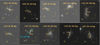 |
Fig. 1. SDSS images of the sample: H011, L024, L084, L097, L115, L125, L127, L156, L170, and L207. The 1 arcsec slit used for the observation is illustrated and the position angle used for each of the observations is marked. Scale is mentioned in each image. North is up and east is to the left. The radio detected galaxy is marked with an ‘r’. |
This paper is organised as follows. We present details about the observations and data reduction in Sect. 2. In Sect. 3, we present all of the sources from the sample and their 1D optical spectra, while the radio data are discussed in Sect. 4. We discuss our findings in Sect. 6. We draw our conclusions and present a summary in Sect. 7.
2. Observations and data reduction
Optical long-slit spectroscopy was conducted for all of the sources using the multi-object double spectrographs (MODS) mounted on the Large Binocular Telescope (LBT; Pogge et al. 2010). The LBT has two 8.4 m mirrors located side-by-side, with a centre-to-centre distance of 14.4 m. The MODS are a pair of seeing-limited, two-channel, identical spectrographs, with low-to-medium resolution. They are mounted on the twin mirrors of the LBT. A dichroic splits the light into blue and red optimised spectrograph channels, so that when they are used in binocular mode, there are four sets of 2D spectra for each exposure. The LBT has a field of view of 6′×6′, while the wavelength coverage of MODS extends from 3000 Å to 10 000 Å.
The observations of the ten sources were carried out over several months, starting in January 2020 and ending in May 2021. Table 1 gives an overview of the dates of observations, exposure times, and position angles for the observations. Nearly all sources (except L127) had one position angle; with the slit being centred across both of the nuclei. At each slit position, we took two exposures; one at the zeroth position of the vertical axis and one with a dither of 10″ along the slit to account for any loss of data due to the struts between the slits. Each exposure was 1200 s long. L127 consists of three galaxies. We used two different slit positions to ensure that we could observe the centres of all of them. There were two 900 s exposures at each of the slit positions, centred on the nuclei of the galaxies. L170 has three 600 s exposures centred across the nuclei of both of the galaxies, two exposures at the zeroth position of the vertical axis, and one exposure with a dither of 1″ along the vertical axis of the slit. For all of the observations, the slit used was 1″ wide, with spectral resolution of 150 km s−1 and spatial resolution of 0.627″.
Observational details.
The observed two-dimensional (2D) spectra were flat-fielded and bias corrected using the MODS CCD Reduction pipeline (Pogge 2019) provided by the observatory. Wavelength calibration, background subtraction, flux calibration, and one-dimensional (1D) spectral extraction was performed using pyraf routines adapted from the IRAF manual1 Along with science sources, calibration spectra were also observed. Mercury, neon, argon, xenon, and krypton lamps were observed with the telescope dome closed and used for wavelength calibration. Spectrophotometric standard stars were observed at the start or the end of the night and used for flux calibration. The lamp and spectrophotometric standard star spectra were treated to same data reduction procedures as the science spectra. Fresh calibration data were recorded for each observing run.
3. Spectra of galaxies
In the following section, we present a brief introduction to each of our interacting sources. The 1D spectra are presented, with the prominent emission lines marked, for each of the galactic centre. The values of the flux of each prominent emission line, along with their full widths at half maximum (FWHMs) and line centres, are tabulated. The projected pair separations between the nuclei and the redshift calculated from the emission lines can be found in Tables 2 and 3, respectively.
Projected pair separations.
Redshifts.
3.1. H011
We cross-identified H011 with the archival names of CGCG1033.9+0237, VIII Zw 090, MCG +01-27-019, AKARI J1036322+022144, and CGCG 037-089 using the NASA/IPAC Extragalactic Database2. Located at a Hubble distance of 226.9 Mpc, the galaxy pair appears to have already experienced the first passage of both galaxies. Prominent tidal tails are clearly visible in the SDSS image. The two nuclei seem to be very close to each other in projection, with a projected pair separation of 2.49 kpc. H011 is the source with the shortest projected pair separation in our sample. We designate the brightest centre of the source as H011B and the comparatively less bright source to the south-west of H011B as H011A. The source was observed with a position angle such that both of the nuclei fell on the slit. The slit position has been marked in Fig. 1, along with the positions of nuclei A and B. The 1D spectra of nuclei A and B are shown in Figs. 2 and 3. Both nuclei have several strong emission lines. The emission lines have been marked in the spectra. We used the lmfits module of Python to perform Gaussian fitting for all of the strong emission lines, thereby allowing us to estimate the line centres, FWHMs, and fluxes of the lines. These have been tabulated for nuclei A and B in Tables 4 and 5, respectively.
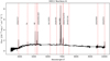 |
Fig. 2. 1D optical spectrum of the H011A nucleus, extracted over an aperture of ∼1.2 arcsec (∼1.2 kpc at given redshift). Prominent emission lines are marked and named. The x-axis represents the wavelength in Angstroms, while the y-axis depicts the flux in units of erg s−1 cm−2 Å−1. The flattened part of the spectrum between 5500 and 6000 Å is the region where the end of the blue channel overlaps with the beginning of the red channel of MODS. Two additional sections beyond 7500 Å have been normalised. They coincide with a sky absorption line and a noisy part of the spectrum. |
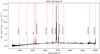 |
Fig. 3. 1D optical spectrum of the H011B nucleus, extracted over an aperture of ∼1.2 arcsec (∼1.2 kpc at given redshift). Prominent emission lines are marked and named. The x-axis represents the wavelength in Angstroms, while the y-axis depicts the flux in units of erg s−1 cm−2 Å−1. The flattened part of the spectrum between 5500 and 6000 Å is the region where the end of the blue channel overlaps with the beginning of the red channel of MODS. Two additional sections beyond 7500 Å have been normalised. They coincide with a sky absorption line and a noisy part of the spectrum. |
H011 nucleus A emission line data.
H011 nucleus B emission line data.
We note two interesting points in the spectra of the two nuclei. First, while the Hα emission line of H011B has a broad component, the broad component is conspicuously missing in the case of the Hβ emission line. Second, while nuclei A and B have comparably similar flux values in the blue channel, with the values of nucleus A being slightly larger than nucleus B, the fluxes of the various emission lines of nucleus B in the red channel are much larger than nucleus A. It could be that the nucleus of H011B is enshrouded in dust, thereby preventing an unimpeded view to the centre.
3.2. L024
L024 can be cross-identified as SDSS J121346.07+024841.4 and IRAS 12112+0305NE using the NASA/IPAC Extragalactic Database3. The source is made up of at least two galaxies and seems to be in a phase post the first passage of the galaxies. Prominent tidal tails are visible in the optical SDSS image, with one tidal tail seemingly going northwards and then turning downwards to the south, while the second tidal tail seems to extend towards the observer inclined edge-on to our line-of-sight (LoS), before turning and extending away from our LoS. The planes described by the tidal tails appear to be mutually perpendicular. The projected pair separation between the nuclei is 5.10 kpc. The brightest centre is designated as L024A, while the source to the south-west of L024A is designated as L024B. Figure 1 shows the slit position used to observe this source, so that both of the nuclei fall onto the slit, and the approximate positions of nuclei A and B are marked as well. The 1D spectra of nuclei A and B are shown in Figs. A.1 and A.2, respectively. Several emission lines are visible in the spectra of both of the nuclei. However, it is clear at close inspection that the spectrum of L024B is slightly noisier than the spectrum of L024A. The various emission lines are marked in the spectra. The values of line centres, FWHMs, and fluxes obtained by performing Gaussian fitting of the emission lines have been tabulated and given in Tables 6 and 7, respectively.
L024 nucleus A emission line data.
L024 nucleus B emission line data.
We note that two narrow components are required to get a good Gaussian fit of the Hα + [NII] complex corresponding to the L024A nucleus. Since we are already past the first passage of the galaxies, it is possible that the massive movement of gas and dust associated with the turbulence of such a major event causes structure in the narrow line region. It could also be possible that narrow line regions corresponding to two nuclei are being probed in the slit position due to the chaotic movement of gas and closeness of the nuclei. Another point of interest is that there seems to be a blue-ward wing associated with the [O III]λ5007 emission line. This could be due to outflows, taking into consideration that the [O III]λ5007 emission line is associated with outflows (Weedman 1970; Heckman et al. 1981; Veilleux & Osterbrock 1987; Harrison et al. 2014).
3.3. L084
L084 was cross-identified with 2MASX J09054734+3747374, WISEA J090547.34+374738.1, and SDSS J090547.33+374738.2 using the NASA/IPAC Extragalactic Database4. The optical SDSS image shows two galaxies. We designate the brightest centre in the source as L084B. The centre of the bluish source to the south-west of L084B we designate as L084A, although we note that it is not particularly distinguishable from L084B in the SDSS fits file. L084 seems to be in the phase past the first passage of the individual galaxies as well, but the tidal tails seem to be in the planes along the LoS and, thus, they are not especially pronounced. The projected pair separation between the nuclei is estimated to be 6.31 kpc. Figure 1 shows the slit position used to observe L084, along with the approximate positions of L084A and L084B.
The 1D spectra of L084A and L084B are shown in Figs. A.3 and A.4, respectively. The spectra of both of the nuclei show several emission lines. However, L084A has a noisier spectrum. Several strong calcium H+K band absorption features are visible in the wavelength range 4000–4300 Å. Additionally, we note that L084A has a bump in the continuum around 4100 Å. We have truncated the spectrum at wavelength 7100 Å since the spectrum is very noisy beyond this and no emission lines are visible. L084B has several more emission lines compared to L084A. The continuum is almost flat for the entirety of the visible wavelength range. The values of the line centres, FWHMs and fluxes obtained from the Gaussian fitting of both of the nuclei can be found in the Tables 8 and 9, respectively. The fluxes of the emission lines belonging the spectrum of L084A are at least an order of magnitude smaller than those of L084B. In the case of L084B, both [O III]λ4959 and [O III]λ5007 have wings. These could be associated with stellar winds or outflows. Additionally, the Hα emission line belonging to L084B has a broad component.
L084 nucleus A emission line data.
L084 nucleus B emission line sdata.
3.4. L097
L097 can be cross-identified as SBS 1123+550, CGCG 268-035, CGCG 1123.6+5503, WISEA J112628.37+544713.8, and 2MASX J11262822+5447138 using the NASA/IPAC Extragalactic Database5. The source is made up of two galaxies that seem to be approaching each other. A bluish spiral galaxy seems to host the brightest centre of the source, which we have designated as L097A. The second nucleus, designated L097B, is hosted in a yellowish, seemingly spheroidal galaxy to the south-east of L097A. Along with these two galaxies, there are two other sources that appear to be close to L097 in projection; a spiral bluish galaxy to the north-west of L097A and a yellow spheroidal galaxy to the west of L097A. In this work, we focus only on L097 and the two nuclei associated with it. L097A and L097B have a projected pair separation of 7.19 kpc. Figure 1 shows the slit position used to observe L097, with the approximate positions of the two nuclei marked as well.
The 1D spectra of L097A and L097B are shown in Figs. A.5 and A.6, respectively. L097A has several strong emission lines. Some calcium H+K band absorption features are visible, as well. Several emission lines corresponding to the Balmer recombination series are visible. Compared with Hβ, the [O III]λ4959 and [O III]λ5007 lines appear to be quite weak. L097B has a less bright spectrum. It is also noisier in comparison with L097A and has fewer emission lines. The Hα recombination line seems to be weaker than the [N II]λ6583 emission line. The ratio of the fluxes of Hβ recombination line to the [O III]λ5007 emission line for L097B would be higher than a similar ratio for L097A. The ratio Hα/Hβ, ∼0.86 is lower than the theoretically expected value of 2.8 for case B recombination in HII regions (Miller 1974). We have truncated the spectrum of L097B at approximately 7100 Å, since the spectrum becomes very noisy and no emission lines are visible. The strongest emission line in the spectrum of L097B is the [O II]λ3727 emission line, with the ratio log([O II]λ3727/Hα) ∼ 0.47. In general, the blue channel spectrum of L097B is brighter than the red channel spectrum. The values of the line centres, FWHMs and fluxes obtained from the Gaussian fitting of both of the nuclei can be found in Tables 10 and 11, respectively.
L097 nucleus A emission line data.
L097 nucleus B emission line data.
3.5. L115
Cross-identified as UGC 04653, ARP 195, VV 243, CGCG 180-018, and CGCG 0850.7+3520 using the NASA/IPAC Extragalactic Database6, L115 is made up of three galaxies that are interacting with each other. The brightest nucleus is hosted by the central galaxy and is designated as L115B by us. The nucleus of the galaxy to the south of L115B is designated as L115A, while the nucleus to the north of l115B is L115C. The galaxy hosting L115A is a face-on spiral galaxy with a bright core. The host galaxy of L115B seems to be edge-on and it is unclear whether this is an early or late type galaxy. The galaxy hosting L115C seems to be a late type spiral, with a prominent tidal tail extending far out in the north-west direction from the host galaxy. The projected pair separation between l115A and L115B is 19.00 kpc; between L115B and L115C, it is 14.56 kpc; and between L115A and L115C, it is 33.92 kpc. Figure 1 shows the slit position used to observe the source. The approximate positions of L115A, L115B and L115C are marked therein, as well. The 1D spectra of the three nuclei can be studied in Figs. A.7–A.9, respectively.
L115A and L115B have several strong emission lines. While L115B has a relatively strong [S III]λ9069 emission line towards the end of the red channel, this is not visible in the L115A spectrum, which has been truncated here since the spectrum becomes very noisy beyond 7500 Å. L115B has a stronger red component compared to its blue component. This is less pronounced in the case of L115A. L115C has a very faint spectrum in comparison with L115A and L115B. Fewer emission lines are visible over the noisy continuum, with Hα and [O II]λ3727 being the strongest emission lines in the spectrum. The edge-on view to the centre of the galaxy might be responsible for enshrouding the central regions, thereby giving rise to a noisy and faint spectrum. The process of interacting with other galaxies also causes violent movement of gas and dust within the galaxies, which might lead to the obscuration of the central object. The values of the line centres, FWHMs and fluxes obtained from the Gaussian fitting of all three of the nuclei can be found in Tables 12–14, respectively.
L115 nucleus A emission line data.
L115 nucleus B emission line data.
L115 nucleus C emission line data.
3.6. L125
We cross-identified L125 with 2MASX J09170001+0926486, SDSS J091659.97+092648.6, GALEXASC J091659.82+092648.0, IRAS 09143+0939, and IRAS F09143+0939 using the NASA/IPAC Extragalactic Database7. L125 is made up of two edge-on disk galaxies with a projected pair separation of 4.48 kpc. The brightest nucleus in the source is designated as L125B, while the second nucleus to the south-west of L125B is designated as L125A. The optical SDSS image in Fig. 1 shows the approximate positions of the two nuclei. The slit position used to observe the source is drawn, as well. L125A sits in the centre of a rather blue host galaxy, while L125B is hosted by a redder galaxy. This is reflected in the 1D optical spectra of L125A and L125B, shown in Figs. A.10 and A.11, respectively.
L125A has a rather flat continuum with very strong emission lines. The emission lines in the blue channel are stronger than the emission lines in the red channel. L125A shows very weak [N II]λ6548 and [N II]λ6583 emission lines, along with very strong [O III]λ4959 and [O III]λ5007 emission lines and recombination lines up to H8 in the hydrogen Balmer series. L125B has a more typical spectrum, with a slight rise in the continuum towards longer wavelengths. Several strong emission lines are visible. The red channel has a stronger emission than the blue channel. The [N II]λ6548 and [N II]λ6583 emission lines are relatively stronger in L125B compared to L125A. In the blue channel of L125B, the [O III]λ4959 and [O III]λ5007 emission lines are weaker than the Hβ recombination line. Both of the nuclei have clearly distinguishable [S III]λ9069 and [S III]λ9531 emission lines at the end of the red channel. The values of the line centres, FWHM, and fluxes obtained from the Gaussian fitting of both of the nuclei can be found in the Tables 15 and 16, respectively.
L125 nucleus A emission line data.
L125 nucleus B emission line data.
3.7. L127
L127 consists of three galaxies interacting with each other. It has been cross-identified with CGCG 063-051, CGCG 0940.7+1019, MCG +02-25-024, 2MASX J09432129+1005128, and 2MASS J09432131+1005129 using the NASA/IPAC Extragalactic Database8. The brightest centre in the source is designated as L127B. The source to its north-west is designated as L127A, while the source to its north-east is designated as L127C. We managed to perform long-slit spectroscopy on all three sources using two different slit positions. Figure 1 shows the optical SDSS image of L127 with the two slit positions drawn and the approximate positions of all three nuclei marked. The projected pair separation between L127A and L127B is 13.26 kpc, between L127B and L127C is 8.99 kpc, and between L127A and L127C is 15.21 kpc, respectively. L127A is hosted by a face-on spiral galaxy. The host galaxy of L127B seems to be a red spheroid, while L127C sits at the centre of a very blue irregularly shaped galaxy. It might be that L127C has already suffered distortions due to previous encounters. The optical 1D spectra of L127A, L127B and L127C are shown in Figs. A.12–A.14, respectively.
L127A has a weak optical spectrum. Only a few emission lines are visible, primarily: the Hα + [NII] complex, the [O II]λ3727 emission line, the [S II]λ6716, [Ar III]λ7136 doublet, and the Hβ recombination line. The [O III]λ4959 and [O III]λ5007 emission lines are very weak. The continuum seems to be rise towards longer wavelengths. The spectrum has been truncated around 7100 Å as there are no emission lines visible beyond this point and the spectrum becomes noisy. The spectrum of L127B is the brightest. Several strong emission lines are visible, with the Hα + [NII] complex in the red channel being the strongest lines. The hydrogen recombination Balmer series is visible until Hϵ. The continuum seems to be flat. L127C has a bright spectrum, as well. It is stronger in the blue channel as compared to the red channel. Several strong emission lines are visible, the [O III]λ5007 emission line being the strongest throughout the spectrum. In the red channel, the Hα + [NII] complex is the strongest. The hydrogen recombination Balmer series is visible clearly until H8. The continuum seems to be flat throughout the spectrum. The [S III]λ9069 emission line is clearly visible for L127B and L127C at the end of the red channel. The values of the line centres, FWHMs and fluxes obtained from the Gaussian fitting of all three of the nuclei can be found in the Tables 17–19, respectively.
L127 nucleus A emission line data.
L127 nucleus B emission line data.
L127 nucleus C emission line data.
3.8. L156
L156 can be cross-identified as UGC 04947, CGCG 181-026, CGCG 0916.9+3308, MCG +06-21-016, and B2 0916+33 using the NASA/IPAC Extragalactic Database9. The source (see Fig. 1) consists of two spiral galaxies interacting with each other. We designate the brightest centre of the galaxy as L156B, with the other centre to the south-east of it being designated as L156A. Prominent tidal tails are visible, such that the system might be in the phase post the first passage of the individual galaxies. The projected pair separation between the nuclei is 5.50 kpc. The 1D optical spectra of L156A and L156B are shown in Figs. A.15 and A.17, respectively.
The spectrum of L156A has several strong emission lines, with the Hα + [NII] complex being the strongest lines in the spectrum. Interestingly, the Hα recombination line needs two narrow Gaussian components for the fit to be good. A zoom-in view on the Gaussian fit of the Hα + [NII] complex of L156A can be seen in Fig. A.16. We also note that both the [O III]λ4959 and the [O III]λ5007 emission lines show a blue-ward asymmetry. The continuum rises towards the longer wavelengths in the blue channel before flattening in the red channel. L156B has a brighter spectrum than L156A, especially with respect to the Hα + [NII] complex. The hydrogen recombination Balmer series extends up to Hδ for both of the nuclei in the blue channel, however, unlike L156A, L156B does not show asymmetry in the structures of the [O III]λ4959 and the [O III]λ5007 emission lines. Similarly to L156A, the Hα recombination line must be fit using two narrow Gaussian components to get a good fit. The optical image of L156 shows that the two galaxies are quite close to each other in projection and it is difficult to distinguish between them in the regions between the two nuclei. The movement of gas and dust caused by the interaction between the two galaxies could be responsible for the dual components of the narrow Hα recombination line. The values of line centres, FWHM, and fluxes obtained by performing Gaussian fitting of the emission lines have been tabulated and given in Tables 20 and 21, respectively.
L156 nucleus A emission line data.
L156 nucleus B emission line data.
3.9. L170
We cross-identified L170 as VV 705, MRK 0848, I Zw 107, CGCG 221-050, and CGCG 1516.2+4255 using the NASA/IPAC Extragalactic Database10. It consists of two spiral galaxies that have already finished the first passage against each other. We denote the brightest nucleus in the source as L170B, while the second nucleus to the south-east of L170B, we label as L170A. The tidal tails associated with both of the galaxies are very prominent. The tidal tail of L170A seems to move southwards before turning north-westwards. Meanwhile, the tidal tail associated with L170B moves up and out westwards from the galaxy before turning southwards and then to the east behind the host galaxy of L170B. The optical SDSS image of L170, along with the slit position and the approximate positions of L170A and L170B are shown in Fig. 1. The projected pair separation between the two nuclei is estimated to be approximately 4.86 kpc. Figures A.18 and A.19 show the 1D optical spectra of L170A and L170B, respectively.
The optical spectra of both L170A and L170B show several strong emission lines. The spectrum of L170B is brighter than that of L170A. Both of the nuclei have distinguishable Balmer emission until Hγ. Both of the nuclei have broad components in the Hα recombination line. However, in the case of L170B, both the [O III]λ4959 and the [O III]λ5007 emission lines show asymmetry in their structure, unlike L170A. The [S III]λ9069 and the [S III]λ9531 emission lines are stronger for L170B as compared to L170A. The continuum seems to rise towards longer wavelengths for L170A, while it is flatter for L170B. The values of line centres, FWHMs and fluxes obtained by performing Gaussian fitting of the emission lines have been tabulated and can be found in Tables 22 and 23, respectively.
L170 nucleus A emission line data.
L170 nucleus B emission line data.
3.10. L207
L207 can be cross-identified as UGC 04090, CGCG 087-046 NED2, MCG +03-02-016 NED02, and 2MASXi J0754322+164835 using the NASA/IPAC Extragalactic Database11. The source (see Fig. 1) consists of a face-on spiral galaxy interacting with a seemingly edge-on disc galaxy. We designate the first galaxy along the slit, the southern-most galaxy, as L207A. The brighter galaxy to the north-east is designated as L207B. The projected pair separation between the nuclei is 13.34 kpc. The galaxies seem to already be in the process of interacting with each other, as evidenced by the presence of strong tidal tails, that are ubiquitous in the case of such events. The 1D optical spectra of L207A and L207B are shown in Figs. A.20 and A.21, respectively.
Both 207A and L207B have similarly noisy spectra, but display several emission lines. For the case of L207A, the Hα + [NII] complex is the brightest, followed by the [O II]λ3727 emission line. Several stellar absorption lines are visible in the spectrum of L207A, especially in the wavelength range 3910–4350 Å. The spectrum of L207B displays emission lines similar to L207A with the notable addition of a broad Hα recombination line component. In contrast to L207A, the [O III]λ4959 and the [O III]λ5007 emission lines are stronger than the Hβ recombination line. L207B displays stronger levels of ionisation compared to L207A. The values of line centres, FWHM, and fluxes obtained by performing Gaussian fitting of the emission lines have been tabulated and are given in Tables 24 and 25, respectively.
L207 nucleus A emission line data.
L207 nucleus B emission line data.
3.11. General comments on the spectra of sample galaxies
The optical spectra of the nuclear regions of all galaxies in our sample show several emission lines, some more so than others. The most common, and usually the most prominent lines are the Hα and the Hβ recombination lines, along with the [O II]λ3727 and the [O III]λ5007 ionisation lines. These line emissions trace star formation, but could also indicate the activity of the central BH. We study this in some detail by using diagnostic diagrams in Sect. 6.2.
H011B, L084B, L170A, L170B, and L207B have broad Hα components in their spectra. However, the broad components appear to be missing from the Hβ line. It could be that the broad component is masked by an absorption feature that overlays the emission line. The presence of the broad component in the spectra of these galaxies indicates the presence of a broad line region (BLR) associated with an active SMBH.
The asymmetric [O III]λ5007 emission line is known to be a tracer of outflows. Outflows are seen to be present in galaxies hosting AGNs as well as star forming regions (Harrison et al. 2014; Bae & Woo 2016; Cicone et al. 2016; Kakkad et al. 2016; Zakamska et al. 2016; Matzko et al. 2022). Since mergers cause a movement of material within galaxies, it would not be surprisingly to see a large incidence of outflows within our sample. However, this is not exactly the case. Amongst our sample, we see that L024B, L084B, L125B, L156A, and L170B have winged [O III]λ5007 emission line. All of these galaxies with the asymmetric [O III]λ5007 emission are detected at 1.4 GHz in the FIRST survey (see Sect. 4 for a detailed discussion on the radio data of the sample). However, not all of the radio detected galaxies have asymmetric [O III]λ5007 emission. This result is consistent with, for instance, Matzko et al. (2022), who found that the merging environment does not predominantly impact the incidence of outflows in galaxies.
Another point of interest is the presence of [S III]λ9069 and [S III]λ9531 emission lines in the spectra of some of the galaxies. We are able to detect these emission lines due to the wavelength coverage of the LBT that extends up to 10 000 Å in the red channel. [S III]λ9069 is detected in H011A, H011B, L024B, L084B, L115B, L125A, L125B, L127B, L127C, L156A, L156B, L170A, and L170B, while [S III]λ9531 is seen in H011A, H011B, L084B, L097A, L125A, L125B, L156A, L156B, L170A, and L170B.
The continua underlying the spectra may be analysed to understand the nature of the host galaxies. Most of the galaxies in our sample show a mild increase towards the red part of the spectrum. This is most likely due to contributions from the obscuring dust and starlight. This can be seen most prominently in the case of L115C, and to some degree in the spectra of L097B, L127A, L207A, and L207B. The spectrum of L084A stands out in the sample, since this is the only galaxy whose spectrum shows a quasar-like shape, especially with a feature that closely resembles the big blue bump. Linearly fitting the blue and red continua separately and using the expression, αλ = −(αν + 2), from Vanden Berk et al. (2001) to convert from wavelength to frequency regime, gives a slope of −1.9834±0.0002 for the blue part and −1.9949±0.0003 for the red part. Comparing this to power law fitting and spectral slopes of −0.44 and −2.45 quoted by Vanden Berk et al. (2001) for the blue (∼ 3000 − 5000 Å) and red (≥ 5000 Å) parts of the spectrum, we see that while the spectral slopes are very different for the blue part, they are consistent for the red part. Additionally, the overall shape of the spectrum of L084A resembles the composite quasar spectrum. The difference in the spectral slopes might arise from contributions from starlight.
4. Radio data
While we have not performed any fresh radio observations, we had access to previously conducted continuum observations using the Effelsberg radio telescope at 4.85 GHz and 10.45 GHz. Additionally, for each of the sources, we made use of observations at 1.4 GHz from the FIRST survey. We adopted the spectral slope values from the continuum observations done using the Effelsberg radio telescope as quoted in Zajaček & Busch (2019). Details about the SDSS-FIRST cross identification, as well as the Effelsberg observations at 4.85 GHz and 10.45 GHz can be found in Vitale et al. (2012, 2015) and Zajaček & Busch (2019). Figure 4 shows the SDSS images of all of the sources with arbitrarily defined SDSS contours in red, overlaid by arbitrarily defined FIRST contours in green. The FIRST database lists the closest SDSS source within a radius of 30″ of the radio source. This helped us to determine which galaxy or nucleus to associate with the dominant radio emission. Exact identification is tricky in the cases of H011 and L024, since these sources are compact enough at optical wavelengths that the radio map at 1.4 GHz encapsulates both of the galaxies when they are overlaid, as can be seen from the Fig. 4. We have associated the radio emission with the galaxy identified by FIRST to be the closest to the radio detection. The radio spectral index of each source estimated from their flux densities at 1.4 GHz and 4.85 GHz can be found in the second column of Table 26. We used the following convention to classify the sources as steep, flat, or inverted, based on the values of their radio spectral slopes:
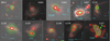 |
Fig. 4. SDSS (aperture size ∼3″) contour images of all sources overplotted with FIRST (angular resolution ∼5″ contours). The contour levels are chosen arbitrarily. SDSS contours are in red, while the FIRST contours are indicated with the colour green. North is up and east is to the left. Scale is indicated in each image. |
Radio-loudness and spectral indices.
(i) α ≤ −0.7: steep,
(ii) −0.7 ≤ α ≤ −0.4: flat,
(iii) α ≥ −0.4: inverted.
We do not consider the Effelsberg observations at 10.45 GHz studied in Vitale et al. (2015) and Zajaček & Busch (2019) in this work, since only H011 and L170 are detected at this frequency. Following the discussion in Zajaček & Busch (2019), we define the radio-loudness parameter of a source as the ratio of the radio flux density to the optical flux density. We used the flux density values of the galaxies at 20 cm (F1.4), which are available from the FIRST survey, and converted the radio flux density into the ABν-radio magnitude system (Oke & Gunn 1983), using the following conversion (Ivezić et al. 2002):
 (1)
(1)
where 3631 Jy is the wavelength-independent zero point. The radio-loudness parameter, Rg, can then be estimated as:
 (2)
(2)
where g signifies the optical g-band magnitude for each source, as quoted in the SDSS-DR7 catalogue. The radio-loudness parameter values for each galaxy, estimated using this method, can be found in the third column of Table 26.
However, with an aperture size of 3 arcsec, the optical flux density from SDSS corresponds to the host galaxy and not just the nucleus of the galaxy. As a result, the radio-loudness parameter thus defined represents the ratio of the radio emission from the centres of the galaxies to the optical g-band emission from the host galaxies. In a bid to understand how the radio emission behaves with respect to the optical emission from the centres of the galaxies, we estimated the radio-loudness as the ratio of the luminosity of the source at 1.4 GHz to its optical continuum luminosity at 5100 Å. The optical luminosity is estimated over an aperture of 1.2 arcsec. The radio-loudness parameters estimated with this method can be found in the fourth column in the Table 26. As a comparison, we estimated the corresponding radio-loudness parameter using the optical continuum luminosity at 5100 Å from the SDSS spectra, these can be found in the fifth column of the Table 26. For the purpose of analysis, we used R > 10 (e.g., Kellermann et al. 1989) as the criterion to classify a source as radio-loud based on LBT data.
The values of the radio-loudness parameter estimated using the continuum luminosity from the SDSS spectra are comparatively lower than the values calculated using the LBT spectra. The reason for this is that the aperture size of SDSS is more than twice that used to extract the LBT spectra. This in turn leads to higher luminosity estimates for the SDSS spectra, and thus lower values of R. On the basis of the adapted criterion, H011A is the only radio-loud galaxy, while the others, despite being radio detected still have lower radio-loudness parameters.
5. Mid-infrared data
In order to take into consideration the mid-infrared (MIR) properties of the galaxies within our sample, we made use of the data observed by WISE in the W1, W2, W3, and W4 bands, corresponding to 3.4 μm, 4.6 μm, 12 μm, and 22 μm respectively. Furthermore, we computed the source flux density in Jansky (Jy) units from the WISE Vega magnitude of the galaxies in the W3 band, m12 μm, using the following equation:
![Mathematical equation: $$ \begin{aligned} F_\nu [\mathrm{Jy}] = F_{\nu 0} \times 10^{(-m_{12\,\upmu \mathrm{m} }/2.5)}, \end{aligned} $$](/articles/aa/full_html/2023/03/aa44721-22/aa44721-22-eq3.gif) (3)
(3)
where Fν0 is the zero magnitude flux density corresponding to the constant that gives the same response as that of Vega, and has a value of 31.674 for the W3 band. We use the computed flux density to further estimate the 12 μm luminosity of the galaxies in the units of erg s−1.
Table 27 lists all of the galaxies detected by WISE, their Vega magnitudes in the four bands, and luminosity at 12 μm. With the exception of L170A, all galaxies that either host a nuclear region that has broad emission line components in its spectrum or are detected at 1.4 GHz in the FIRST survey are also detected by WISE.
MIR luminosity data.
6. Discussion
All of the galaxies presented in Sect. 3 have emission lines that can be analysed to study the nature of the regions where they originate. In this section, we discuss the properties showcased by the interacting systems in our sample. We start by briefly describing our estimates for the masses of the SMBHs hosted by the galaxies. We follow by plotting diagnostic diagrams, such as the BPT diagram proposed by Baldwin, Phillips, and Terlevich (Baldwin et al. 1981). The diagnostic diagrams are used to identify whether the emission lines arise in a hard-ionising field associated with AGNs or a softer ionising field that characterises star formation, based on the ratios of emission lines that are placed close to each other in the spectrum, so that we may safely disregard reddening and do not need to correct for interstellar and galactic extinction (Kewley et al. 2019). Furthermore, we discuss the optical and radio properties of the galaxies in the context of their luminosities, ionisation ratios, Eddington ratios, radio-loudness parameters, and radio spectral indices.
6.1. Masses of the central super massive black holes
Optical spectra of nuclear regions of a galaxy are useful in the estimation of the masses of the central SMBH. This can be accomplished either by estimating the stellar velocity dispersion of the galaxy or, given the presence of broad emission lines in the spectrum, by making use of the virial theorem.
We used the penalised pixel-fitting (pPXF) method (Cappellari & Emsellem 2004; Cappellari 2017) to fit stellar components (Sánchez-Blázquez et al. 2006; Vazdekis et al. 2010; Falcón-Barroso et al. 2011) to our galaxy spectra, thereby estimating the values of their stellar velocity dispersion. The values of the stellar velocity dispersion corresponding to each of the galaxy can be found in Table 28. For H011B, L024B, L125A, and L127C, pPXF was not able to fit a reasonable stellar component, either because the continuum was too strong or because the spectrum was too noisy or attenuated.
Stellar velocity dispersions.
We use the M-σ relation presented by Gültekin et al. (2009):
![Mathematical equation: $$ \begin{aligned} \log (M_\mathrm {SMBH} ) = 8.12 + \Bigg [4.24\times \log \Bigg (\frac{\sigma }{200}\Bigg )\Bigg ] \end{aligned} $$](/articles/aa/full_html/2023/03/aa44721-22/aa44721-22-eq4.gif) (4)
(4)
to estimate the masses of the SMBHs at the centres of the galaxies with an estimated stellar velocity dispersion value. These can be found tabulated in the Table 29.
Masses of the supermassive black holes.
While we could not determine a stellar velocity dispersion for H011B, it has a broad Hα component, we used the FWHM of this broad component to estimate mass of the central SMBH using the virial theorem (Greene & Ho 2005; Peterson 2010; Woo et al. 2015):
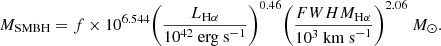 (5)
(5)
We adopt the value of 1.12 for the factor f (Woo et al. 2015) and estimate the black hole mass to be (1.027 ± 0.051)×107 M⊙. The value in its logarithmic form is also listed in Table 29. L207 B has a broad Hα component as well as stellar absorption features. As a result of this, we were able to estimate the black hole mass for this nucleus using both of the methods. The logarithm of the BH mass using stellar velocity dispersion is estimated to be (5.834 ± 0.052)×107 M⊙, while it is (4.188 ± 0.262)×107 M⊙ using the FWHM of the broad Hα component. For consistency with the method of mass estimation for most of the sample of galaxies, we state the value estimated using the stellar velocity dispersion in Table 29.
A look at the values in Table 29 shows that almost all of the SMBHs have masses in the range 106 − 108 M⊙, which is the typical range for BH masses in quasars. Especially, all of the galaxies associated with radio emission, with the exception of L084B, host central SMBHs with values of mass in the multiples of 108 M⊙.
Amongst the galaxies not detected in the radio regime, there is one exception; L084A has a BH mass of (9.19 ± 0.021)×105 M⊙, which is on the low end of the mass range of SMBHs. L084A appears extremely blue in the optical SDSS images, and has strong [O III] emission and Hα recombination lines. So, L084A could be a compact, young, star-forming galaxy, with the gas reservoir being used mostly for star formation as opposed to accretion on to the central BH and leading to a less massive BH. We note that it is difficult to understand properly the morphology of the pair, since the region between the two galaxies is rather ambiguous. As a result, it could be that we underestimate the value of the mass of the SMBH.
6.2. Diagnostic diagrams
For our analysis, we use the [O III]λ5007/Hβ versus the [N II]λ6583/Hα plot (Baldwin et al. 1981), better known as the BPT plot, along with the [O III]λ5007/Hβ versus [S II]λ6716+[S II]λ6731/Hα and the [O III]λ5007/Hβ versus the [O I]λ6300/Hα plots (Veilleux & Osterbrock 1987). Figure 5 shows all three diagnostic diagram plots for the sample of ten interacting sources. Then we use Eqs. (6)–(8) (Groves & Kewley 2008):
![Mathematical equation: $$ \begin{aligned} \log ([{\text{O}}{\small {{\text{ III}}}}]/\mathrm H\beta )&= 0.61/{(\log ([{\text{N}}{\small {{\text{ II}}}}]/\mathrm H\alpha ) - 0.47)} + 1.19,\end{aligned} $$](/articles/aa/full_html/2023/03/aa44721-22/aa44721-22-eq6.gif) (6)
(6)
![Mathematical equation: $$ \begin{aligned} \log ([{\text{O}}{\small {{\text{ III}}}}]/\mathrm H\beta )&= 0.72/{(\log ([{\text{S}}{\small {{\text{ II}}}}]/\mathrm H\alpha ) - 0.32)} + 1.30), \end{aligned} $$](/articles/aa/full_html/2023/03/aa44721-22/aa44721-22-eq7.gif) (7)
(7)
![Mathematical equation: $$ \begin{aligned} \log ([{\text{O}}{\small {{\text{ III}}}}]/\mathrm H\beta )&= 0.73/{(\log ([{\text{O}}{\small {{\text{ I}}}}]/\mathrm H\alpha ) + 0.59)} + 1.33, \end{aligned} $$](/articles/aa/full_html/2023/03/aa44721-22/aa44721-22-eq8.gif) (8)
(8)
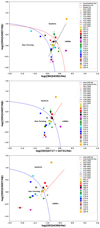 |
Fig. 5. Plots of log([O III]λ5007/Hβ) vs. log([N II]λ6583/Hα), log([O III]λ5007/Hβ) vs. log([S II](λ6717+λ6731)/Hα) and log([O III]λ5007/Hβ) vs. log([O I]λ6300/Hα). Each colour marks a particular interacting pair or group. The inverted triangles represent the data points corresponding to nucleus A of a given source, whereas the squares represent the nucleus B, filled circles represent nucleus C, where applicable, and the crosses mark the data point derived from the SDSS spectrum of the source. The data points have been calculated for an aperture of 1 arcsec. The error bars have been derived from the 1σ standard uncertainty values. |
to define the demarcation curve that separates the line ratios arising from AGNs from the line ratios associated with star-forming regions.
The [O III]λ5007/Hβ versus the [N II]λ6583/Hα plot displays, in addition to the delineation curve defined by Eq. (6), another demarcation curve, as proposed by Kauffmann et al. (2003a), called the ‘pure star-forming’ line. This curve can be defined by Eq. (9) as follows:
![Mathematical equation: $$ \begin{aligned} \log ([{\text{O}}{\small {{\text{ III}}}}]/\mathrm H\beta ) = 0.61/(\log ([{\text{N}}{\small {{\text{ II}}}}]/\mathrm H\alpha ) - 0.05)) + 1.3. \end{aligned} $$](/articles/aa/full_html/2023/03/aa44721-22/aa44721-22-eq9.gif) (9)
(9)
The pure star-forming line is based on observational data, whereas the curve described by Eq. (6) is based on theoretical modelling presented in Kewley et al. (2001) and called the ‘maximum starburst’ line. If a source falls above the maximum starburst curve, the source of ionisation is very strong and could be from the extremely energetic AGN. If the source falls below the pure star-forming curve, the ionising field is soft and could arise from star-forming regions. If an object falls in the region between the two curves on the BPT diagram, the ionisation field could have contributions from an AGN as well as star-forming regions; therefore, it is declared to be a composite or a transitioning object.
The AGN region of all three diagnostic diagrams can be further divided into two separate sub-regions, line ratios arising from the Seyfert type II sources and those ionised by low ionisation nuclear emission-line regions (LINERs). These lines are defined by Eqs. (10) and (11) as follows:
![Mathematical equation: $$ \begin{aligned} \log ([{\text{O}}{\small {{\text{ III}}}}]/\mathrm H\beta )&= 1.89\log ([{\text{S}}{\small {{\text{ II}}}}]/\mathrm H\alpha ) + 0.76,\end{aligned} $$](/articles/aa/full_html/2023/03/aa44721-22/aa44721-22-eq10.gif) (10)
(10)
![Mathematical equation: $$ \begin{aligned} \log ([{\text{O}}{\small {{\text{ III}}}}]/\mathrm H\beta )&= 1.18\log ([{\text{O}}{\small {{\text{ I}}}}]/\mathrm H\alpha ) + 1.30. \end{aligned} $$](/articles/aa/full_html/2023/03/aa44721-22/aa44721-22-eq11.gif) (11)
(11)
The topmost panel in Fig. 5 shows the [O III]λ5007/Hβ versus the [N II]λ6583/Hα plot for all of our nuclei. 13 out of 22 of our nuclei fall in the composite region on this plot. All of them show signs of previous interactions, with the presence of prominent tidal tails. The sources with low line ratios, L127 A, L097 A, and L156 B are hosted by face-on spiral galaxies. In the case of L127, especially, it is difficult to ascertain whether previous interactions have taken place. The source does not exhibit any overt signs of tidal interactions yet. The galaxies are close to each other in projection and redshift, though, so we might be looking at a system that is about to start interacting, with the first processes just starting. L127B and L127C look like there might be some interaction happening already. While L127 A sits below the purely star-forming line, L127 B straddles the line between the line distinguishing the star-forming region from the composite region. L127 C, which appears extremely blue in the optical SDSS image, meanwhile falls below the pure star-forming line, as well, but with a relatively higher [O III]λ5007/Hβ line ratio.
In the case of L097, the nucleus B, lies well inside the LINER region. Its [N II]λ6583 emission line appears to be stronger than the Hα recombination line in its spectrum, as seen in Fig. A.6. The source appears to have reddish centres in the optical SDSS image and might have low amounts of gas to be ionised. Shocks could also be responsible for driving the line ratios that fall in the LINER region (e.g., Farage et al. 2010).
L156 certainly presents tidal tails and a seemingly chaotic environment. It is difficult to gauge whether there are two or three galaxies interacting with each other here. We have studied the nuclear regions of two, but not the third core that appears to the west of nucleus B. It would be interesting to study this and check whether it is really a part of the interaction or whether it is a foreground object. While the nucleus B has a low [O III]λ5007/Hβ line ratio and lies in the star-forming region of the BPT diagram, nucleus A seems to have sufficiently high line ratios to be deemed a composite.
The middle and the bottom panels of Fig. 5 show the [O III]λ5007/Hβ versus [S II]λ6716+[S II]λ6731/Hα and the [O III]λ5007/Hβ versus the [O I]λ6300/Hα plots, respectively. The [O III]λ5007/Hβ versus [S II]λ6716+[S II]λ6731/Hα plot is perhaps the more reliable of the two, since the [S II]λ6716 and the [Ar III]λ7136 emission lines are strong and well-defined for all of our sources. All except the data point associated with L125 A lie in regions similar to the ones in the [O III]λ5007/Hβ versus the [N II]λ6583/Hα plot. This could be because the [N II]λ6583 emission line is curiously stunted in the L125 A spectrum. The galaxy appears very blue in the optical SDSS image. Moreover, it is partially obscured by its companion, L125 B. As a result, it is not certain whether or not we are actually probing the nuclear region of L125 A.
The [O III]λ5007/Hβ versus the [O I]λ6300/Hα plot has fewer data points than the other two plots. This is because the [O I]λ6300 emission line is not sufficiently well defined in the spectra of some of the sources. The data points on the plot correspond to the information gleaned from the [O III]λ5007/Hβ versus [S II]λ6716+[S II]λ6731/Hα plot, however.
6.3. Diagnostic diagrams: trend with radio spectral indices
Figure 6 shows the [O III]λ5007/Hβ versus the [N II]λ6583/Hα plot of the radio detected nuclei with the data points marked by the values of their corresponding spectral indices. Table 26 lists the spectral indices of all of the sources. These values are estimated using the radio fluxes at 1.4 GHz and 4.85 GHz. Almost all of the data points lie in the composite or transitioning region of the BPT diagram, except for the data points corresponding to L097A, which straddles the line separating the composite region from the pure star-forming region, and L207 A, which straddles the line separating the composite region from the LINER region.
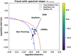 |
Fig. 6. Plot of log([O III]λ5007/Hβ) vs. log([N II]λ6583/Hα) with a colour map based on the radio spectral indices of the sources derived from radio fluxes of the sources at 1.4 GHz and 4.85 GHz. |
Focusing, for now, on the sources that fall in the composite region, we see that most of them, with the exception of L156A, have flat spectral indices. Flat radio spectral indices are associated with a mixture of optically thin and self-absorbed synchrotron emission, associated with radio jets and lobes, respectively. It is difficult to distinguish between the contribution of AGN and star-formation activity towards the overall radio luminosity of a galaxy, since the spectral indices associated with sychrotron emission of supernova remnants are similar to those typical of the radio lobe+jet structures. However, since all of these sources have chaotic environments, typical for interactions of galaxies, there is a good possibility of contribution from an AGN. It would be interesting to see if the AGN is already in a ‘switched-on’ state before the first approach of galaxies or whether the first passage and the movement of gas and dust associated with it is responsible for the switching-on of the central SMBH.
Coming now to L156A and L097A, we see that L156A has the highest spectral index in the sample with a value of 0.3451, while L097A follows with a value of 0.1742. Both of these values fall well in the inverted spectral index range and could be indicative of AGN core components, emanating from self-absorbed synchrotron emission. In the case of L156A, this is reflected in the position of the nucleus on the diagnostic diagram, since it falls very close to the maximum starburst line in the composite region of the BPT diagram (see Fig. 5a), and on the curve dividing the star-forming region from the AGN region on the [O III]λ5007/Hβ versus [S II]λ6716+[S II]λ6731/Hα plot (see Fig. 5b). L097A, however, has very low ionisation ratios, in particular, very low [O III]λ5007 emission. A look at the spectrum of L097A shows that while the Hydrogen recombination line, Hβ, is quite strong, the [O III]λ4959 and the [O III]λ5007 emission lines are quite weak. The centre of L097A seems quite red, which might be indicative of extinction, or the source might have low amounts of ionised material.
The study of interacting galaxies based on the radio spectral index and the optical diagnostic diagrams has some interesting implications. Galaxies in the post-passage phase seem to have flat spectral indices, which are indicative of optically thin synchrotron structures and self-absorbed synchrotron emission, generally associated with the emission from supernova remnants. An increase in star-formation might be linked to the availability of material brought about by the increased movement of gas and dust as the galaxies start interacting with each other. In some cases, perhaps, as in the case of L156A, the AGN is already ignited when the galaxies approach each other; otherwise, it might be the case that age of the interaction leads to the AGN being ignited by the passage and we observe it in the time succeeding the ignition. It could also be that the dusty environment around the centres of the interacting galaxies causes enough obscuration that the diagnostic diagrams are not very reliable, in which case, taking into consideration the radio data of the galaxies could help to understand the nature of the nuclei.
6.4. Diagnostic diagrams: Eddington ratio trend
In order to understand the trend of our galaxies with respect to their Eddington ratio, η ≡ LBol/LEdd (Cavaliere & Padovani 1988), we estimated their bolometric luminosity, LBol, using the equation LBol = kBol × L5100 Å, where kBol is the bolometric correction factor given by kBol = 40 × [L5100 Å/1042 erg s−1]−0.2 (Netzer 2019), and Eddington luminosity, LEdd, where LEdd = 4πGM•mpc/σT = 1.3 × 1038(M•/M⊙) erg s−1 (Lightman 1982). The logarithmic values of LBol, LEdd, and η can be found in the Table 30. We find that all of the radio galaxies, irrespective of their spectral index, have log η values in the range [−4, −2], while the non-radio galaxies span the range [0, −3]. Netzer (2019) uses an optically thick, geometrically thin accretion disc to calculate the optical bolometric correction factor. In the case of H011B, L084B, L170A, L170B, and L207B, the assumption of a standard thin accretion disc is applicable since they show broad components in their spectra, which are typically associated with standard thin discs (Czerny et al. 2004; Czerny & Hryniewicz 2011). In addition, there seems to be no significant trend in the values of Eddington ratios of radio-detected and non-detected sources. Therefore, we conclude that all of our sources might, in principle, have standard discs or discs with mixed properties such that the thin disc transitions to ADAF in the inner regions for lower accretion rates due to the classical ADAF approach (i.e. the hot flow forms whenever it can, see Abramowicz et al. 1995; Honma 1996; Kato & Nakamura 1998) or the disc evaporation model (Liu et al. 1999; Różańska & Czerny 2000; Meyer-Hofmeister & Meyer 2003). In fact, changing-look AGNs, which can be associated with the radiation-pressure instability operating in a radially narrow zone between the ADAF and the thin disc (Sniegowska et al. 2020), exhibit median Eddington ratios of ∼ − 2 (Panda & Śniegowska 2022). Standard thin accretion discs associated with lower accretion rates have been previously reported in, for instance, Bianchi et al. (2019), where a very broad Hα component is found in the spectrum of NGC3137 and the inferred Eddington ratio for this source is log η ∼ −4.
Eddington ratios.
Figure 7 shows the plot of the ionisation ratios, log([O III]λ5007/Hβ), against the Eddington ratios, log η, for the radio detected galaxies. The colour map is defined by using the values of the spectral slope of each of the source. We see that there is no significant trend in the distribution of the spectral indices, as well as Eddington ratios. However, a very weak trend of higher ionisation ratios corresponding to higher values of the Eddington ratio is visible.
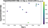 |
Fig. 7. Plot of log([O III]λ5007/Hβ) vs. log η. Colour bar is defined by the value of the spectral index of the source. |
This becomes clearer in Fig. 8, which shows the BPT plot of the radio detected galaxies, with a colour map defined by the logarithmic values of the Eddington ratios.
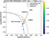 |
Fig. 8. Plot of log([O III]λ5007/Hβ) vs. log([N II]λ6583/Hα) with a colour map based on the value of the Eddington ratio of each source. |
6.5. Ionisation ratio versus radio-loudness parameter
Figure 9 is the plot of the line ratios log([O III]λ5007/Hβ) versus radio-loudness (L1.4 GHz/L5100 @@@(LBT)) parameters of all the radio galaxies. The red dots represent galaxies with inverted spectral indices and green dots indicate galaxies with flat spectral indices. H011A has the highest value of radio-loudness at 22.342, with L115B being second highest at 8.048. L024A and L125B are the lowest at 1.420 and 1.566, respectively.
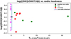 |
Fig. 9. Plot of log([O III]λ5007/Hβ) vs. the radio-loudness parameter (L1.4 GHz/L5100 @@@(LBT)). Green dots represent galaxies with flat radio spectral index (−0.7 ≤ α1.4/4.85 ≤ −0.4), while red dots represent galaxies with inverted radio spectral index (α > −0.4). The vertical blue line represents the median value of the radio-loudness parameter for the non-radio detected galaxies from Table 31 and the magenta arrows indicate that this is the upper limit of the radio-loudness at the log([O III]λ5007/Hβ) values for each of the galaxies. |
If we exclude, for now, H011A from our analysis, we are left with nine radio-quiet galaxies. Three of these have flat spectral slopes, while six have inverted spectral slopes. Considering just the flat sources for now, we see that the ionisation ratio decreases with an increasing radio-loudness parameter, with the spectral slope steepening with increasing radio-loudness parameter. The sources with inverted spectral slopes do not seem to follow a trend with the ionisation ratio and radio-loudness parameter with respect to their spectral slope, but they do seem to cluster at the lower end of the radio-loudness parameter axis.
Coming back to H011A, it is the only galaxy with flux density ≥100 mJy in our sample. It also has the highest radio-loudness parameter, R1.4 GHz/5100 Å(LBT) ∼ 22, considering both LBT and SDSS data (see Table 26), and it is the only radio-loud galaxy in our sample. Marecki et al. (2006) studied H011 using observations with MERLIN at 5 GHz, as a candidate for double-double or X-shaped structures. They refer to the source as TXS 1033+026, and present FIRST and MERLIN maps at 1.4 GHz and 5 GHz, respectively, along with an SDSS image of the source. They infer that the most likely scenario to explain the morphology of the sources is a rapid repositioning of the central engine. Such a rapid repositioning of the central engine could be most likely caused by a merger. They present the following interpretations for the radio maps. In the case of the FIRST map, there is a core that coincides with H011A in the optical domain, and a dominant lobe to the southeast along with either a jet pointing to a second lobe almost 3.5 times away from the core than the southeastern lobe or the protrusion to the northwest itself being the lobe. At 5 GHz, a core and a jet pointing in the northeast direction can be see clearly, along with shorter protrusions to the southeast and northwest, which could be the indicators or ‘remains’ of the flux from the two lobes or the lobe and jet, visible in the FIRST map. The jet at 5 GHz is at an angle of almost 80° relative to the direction of the southeastern lobe at 1.4 GHz12.
Figure 9 can be explained using a simple physical source model as depicted in Fig. 10. Here, we show a possible arrangement of different source components. The radio components are depicted by black contour lines. Radio continuum radiation is indicated by blue arrows, while the ionising optical line emission is indicated by red arrows. The excitation and radio strength parameters are largely independent of each other. The inverted radio flux is due to a compact optically thick jet component that is typically located (due to optical depth effects) a bit upstream from the ionising nucleus (red circle). Excess flat to steep spectrum radio flux density is due to contributions from extended source components like a jet. Steep spectrum contributions could be due to radio lobes or non-thermal supernova remnant emission, as well.
 |
Fig. 10. Underlying physical source model of our interpretation. A detailed description is given in Sect. 6.5. |
In Fig. 11, we make use of the fact that the excitation and radio strength parameters are assumed to be independent of each other, thus, we present a figure that is rather similar to Fig. 9, but the relative contributions of ionising and/or radio detected components are shown continuously in heat colors and black contours. The relative contributions were derived from the median and the approximate extent of the region covered by data shown in Fig. 9. The median position of the radio detected sources is indicated by a black dot. An upper limit of the median position of the radio-weak or non-detected sources is shown by a red hexagram (see also data in the Table 31). The trend indicated here is that the higher ionising sources are also associated with radio bright emission, that is, high values of R. However, the medians also show that the ionising radiation of the radio-detected and weak sources are rather similar, demonstrating that the ionising radiation as such cannot be the only reason for the radio emission of the sources.
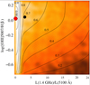 |
Fig. 11. Plot of log([O III]λ5007/Hβ) vs. the radio-loudness parameter (L1.4 GHz/L5100 Å (LBT)), as in Fig. 9, but relative contributions of ionising and/or radio detected components in heat colours and black contours. Radio-loudness parameter is estimated using the 5100 Å luminosity from LBT spectra. |
Radio-loudness parameters and ionisation ratios.
We can compare our LBT source sample with SDSS reference data as presented by Vitale et al. (2015) and Zajaček & Busch (2019). For the radio-detected sources presented there the corresponding scatter plot of ionisation ratio versus radio-loudness is shown in Fig. 12. The median position of the distribution is compatible with the median distribution found in our LBT sub-sample of these sources.
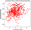 |
Fig. 12. Scatter plot of the reference radio detected source data presented by Vitale et al. (2015) and Zajaček & Busch (2019). Radio-loudness parameter is estimated using the 5100 Å luminosity from SDSS spectra. |
In Fig. 13, we show the same data as in Fig. 12 but collapsed onto the R-parameter axis. We plot the square-root of the number of sources against the radio-loudness parameter using a bin-size of 0.5. The red line shows that there is an excess of radio-loud sources similar to what we find in our sub-sample, albeit at a lower magnitude. The radio-loud sources well above the median position in R are highlighted here by the hashed area. The lower magnitude of the excess is mainly due to the fact that the optical continuum luminosity the radio luminosity is referenced to, is taken in a larger aperture for the SDSS data (approximately 3″) in comparison to the LBT slit width (1″). In the SDSS data, the optical continuum represents the luminosity of the bulge or even the inner section of the host galaxy. In our LBT data we reference the radio luminosity to the nuclear optical continuum within the slit. In fact, multiplying the ratio between the R-values of the radio detected sources to the corresponding limits for the radio weak sources by the upper limit of the excess shown in the distribution in Fig. 13, we obtain a value of about 19. This is in good agreement with the highest R-value of about 22 – as obtained for our SDSS-FIRST-LBT sample.
 |
Fig. 13. Scatter diagram shown in Fig. 12 but collapsed onto the radio-loudness axis (see text in Sect. 6.5). Radio-loudness parameter is estimated using the 5100 Å luminosity from SDSS spectra. |
6.6. Correlations with black hole mass
Next, we looked at any possible correlation between the ionisation ratio of the nuclear regions and the mass of the central SMBHs. Figure 14 shows a scatter plot of the ionisation ratio, represented by log([O III]λ5007/Hβ), versus the logarithmic values of the masses of the central SMBHs. We see no specific correlation between the ionisation ratio and masses of the SMBHs. However, we note that for all of the interacting pairs, with the exception of L156 and L115, it is the galaxy that hosts the more massive SMBH that is associated with the radio detection at 1.4 GHz. In the cases where both of the galaxies are detected at 1.4 GHz, the galaxy with a more massive SMBH has a higher flux density.
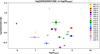 |
Fig. 14. Plot of the ionisation ratio of each galactic nuclear region versus the mass of the central SMBH. The crosses and square represent the masses of the non-radio detected galaxies, while the dots represent the radio detected galaxies. Each interacting pair is represented by a specific colour, as described in the legend of the plot. |
This correlation could be attributed to a more massive circum-nuclear disc being associated with the more massive SMBH, thus providing more material for star-formation and ultimately, radio emission. Additionally, the more massive SMBH could cause stronger emission in the radio regime. It is interesting to note that the values of the radio-loudness parameters of the radio detected sources do not seem to give rise to any correlation in this figure. This can be seen clearly in Fig. 15, which shows the plot of the radio-loudness parameter, estimated using the 5100 Å continuum luminosity from the LBT spectra, against the mass of the central SMBH for all of the radio detected galaxies. We see that there is no obvious correlation between the two properties. This could be related to the stage of the galaxy interaction, with later stages of the collision being associated with stronger radio emission from the AGN, while the earlier phases have weaker radio emission.
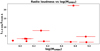 |
Fig. 15. Plot of the radio-loudness parameter of each galactic nuclear region versus the mass of the central SMBH. |
6.7. Correlation with mid-infrared luminosity
Finally, we look at the MIR properties of the galaxies in our sample and study their behaviour with respect to their radio properties. In order to understand the nature of the MIR emission of the galaxies in our sample, we first looked at their W2 − W3 colour, since it is sensitive to the contribution from star-formation. Figure 16 shows the colour-colour plot of W1 − W2 versus W2 − W3. The W2 − W3 values of all of the detected galaxies fall in the range [3.5–4.8], while the W1 − W2 values lie in the range [0.1–1.3]. Herpich et al. (2016) found that the colour W2 − W3 = 2.5 is the best divisor between actively star-forming galaxies and retired galaxies. Galaxies whose star-formation has stopped for a long period of time are classified as retired. Additionally, Stern et al. (2012) showed that the criterion W1 − W2 > 0.8 can be used to identify both unobscured and obscured AGNs. Considering the criteria proposed by Herpich et al. (2016) and Stern et al. (2012) to select AGNs based on the MIR emission, we see that while all of our galaxies have W2 − W3 > 2.5, and are thus likely actively forming stars, only two of them satisfy W1 − W2 > 0.8, namely H011A and L084B. L084B shows broad Hα emission line in its optical nuclear spectrum and as such, already qualifies as a prospective Seyfert 1 galaxy. H011 shows only narrow emission lines in its optical nuclear spectrum and could be a Seyfert 2 galaxy. Alternatively, it could be that the MIR emission is actually associated with H011B, which also has a broad Hα emission line in its optical nuclear spectrum. H011B is separated from H011A by ∼2.4″, while the angular resolution of WISE is 6.1″, 6.4″, 6.5″, and 12″ at 3.4 μm, 4.6 μm, 12 μm, and 22 μm, respectively. The rest of our galaxies seem to lie in the region corresponding to contributions from both star-formation and AGN, including L170B and L207B, both of which have broad Hα emission lines in their nuclear spectra.
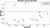 |
Fig. 16. W1 − W2 versus W2 − W3 colour-colour diagram based on the WISE magnitudes at 3.4 μm, 4.6 μm, and 12 μm. The red dots are the data points for the galaxies in our sample. The dashed black line shows the W1 − W2 > 0.8 criterion proposed by Stern et al. (2012). |
Furthermore, we plotted the 12 μm luminosity against the 1.4 GHz luminosity from FIRST data of all WISE-detected galaxies to check for any trend (Fig. 17). We plot the linear regression fitted to this data in a solid blue line. The fit has a positive gradient of 0.36 and an intercept of 35.58. Comparing our plot with the left panel of Fig. 3 in Rosario et al. (2013), we see that our galaxies fall in Branch A, populated by Seyferts and star-forming galaxies, as opposed to Branch B, which is mostly populated by LINERs.
 |
Fig. 17. Plot of log values of the 12 μm luminosity, in erg s−1 units, of the galaxies detected by the WISE W3 band versus the log values of the 1.4 GHz luminosity, in W Hz−1 units, observed in the FIRST survey. The red dots are the data points for the galaxies in our sample. The solid blue line shows the linear regression fit to the data, described by L12 μm = 0.36L1.4 GHz + 35.58. |
7. Conclusions and summary
In this paper, we present the optical spectra of a sample of eights pairs and two triplets of interacting galaxies that have been selected from an SDSS-FIRST parent sample studied in Vitale et al. (2015) and Zajaček & Busch (2019). We observed a total of 22 galaxies using MODS at the LBT, focusing on their central regions. We used continuum data at 4.85 GHz from the Effelsberg telescope as well as FIRST data at 1.4 GHz to estimate spectral slopes and radio-loudness parameters for all of the radio-detected sources. Additionally, we used WISE MIR images at 3.4 μm, 4.6 μm, and 12 μm of the 14 galaxies detected at these wavelengths to plot a W1 − W2 versus W2 − W3 colour-colour diagram and a Lμm versus L1.4 GHz plot. The properties of each pair or triplet are briefly summarised below:
-
H011/CGCG1033.9+0237: The galaxy pair H011 has strongly ionised nuclear spectra. While H011A shows narrow emission lines only, H011B has both broad and narrow components. The pair has the shortest projected pair separation in our sample. Both of the nuclei lie close to each other in the composite region of the BPT diagram. The FIRST radio emission encapsulates both of the galaxies but is centred closest to the H011A nucleus. H011 is the only galaxy pair in our sample with FIRST flux greater than 100 mJy and can be classified as hosting an AGN on the basis of its W1 − W2 colour.
-
L024/SDSS J121346.07+024841.4: The galaxy pair L024 shows prominent emission lines in the spectra of both of the nuclear regions. The FIRST radio emission encapsulates both of the galaxies but is centred closest to the L024A nucleus. L024A has two narrow components corresponding to the Hα emission line. L024B shows a blue wing in its [O III]λ5007 emission line. L024A lies in the composite region of the BPT diagram, while L024B falls in the Seyfert region.
-
L084/2MASX J09054734+3747374: The galaxy pair L084 consists of a blue galaxy L084A in the process of interacting with a red galaxy L084B. The FIRST radio emission is associated with L084B. L084A has a continuum that is quasar, with a blue bump like feature around 4100 Å, along with emission lines. L084B has a flat continuum spectrum, with prominent emission lines. Both [O III]λ4959 and [O III]λ5007 emission lines have blue wings and there is broad Hα component present in the case of L084B. L084B is the only other galaxy other than H011 that can be classified as hosting an AGN on the basis of its W1 − W2 colour. Both of the nuclear regions lie in the composite region of the BPT diagram.
-
L097/2MASX J11262822+5447138: The galaxy pair L097 is a interacting system consisting of a spiral galaxy L097A and a spheroidal galaxy L097B. L097A is associated with FIRST radio emission. The spectrum of the nuclear region associated with L097A has a flat continuum with prominent emission lines but very weak [O III]λ5007 emission, while L097B has a noisier spectrum. Consequently, L097A lies in the star-forming region of the BPT diagram, while L097B lines well within the LINER region.
-
L115/UGC 04653: L115 is a triplet consisting of galaxies L115A, L115B, and L115C in the process of interaction with each other. L115B is detected at 1.4 GHz in the FIRST survey. The spectra of the nuclear regions of L115A and L115B have flat continua with prominent emission lines, while the spectrum of the L115C nucleus is noisy and reddened with weak emission lines. L115A and L115B fall in the composite region of the BPT diagram, while L115C lies in the Seyfert region.
-
L125/2MASX J09170001+0926486: The galaxy pair L125 consists of a blue galaxy L125A and the red spiral galaxy L125B. The FIRST radio emission can be associated with L125B. L125A shows a very flat continuum, while the continuum of L125B shows some reddening. Both the nuclear spectra have prominent emission lines, and show Balmer series lines up to H8 for LL125A and Hδ for L125B. Both [O III]λ4959 and [O III]λ5007 emission lines display blue wings in the nuclear spectrum of L125B. L125A falls in the star-forming region in the BPT diagram, while L125B lies in the composite region.
-
L127/CGCG 063-051: The triplet L127 is made up of a spiral L127A, a spheroidal galaxy L127B, and a blue irregular galaxy L127C interacting with each other. L127B is detected at 1.4 GHz in the FIRST survey. The spectrum of the nuclear region of L127A shows reddening and has weak [O III]λ5007 emission. The nuclear spectra of L127B and L127C have very flat continua. The emission lines in the red part of the spectrum are especially strong for L127B, while the blue band is more prominent in the case of L127C. L127A and l127C lie in the star forming region in the BPT diagram, while L127B falls in the composite region.
-
L156/UGC 04947: L156 is a galaxy pair consisting of a spiral galaxy L156A and a spheroidal galaxy L156B. L156A is visible at 1.4 GHz in the FIRST survey. The nuclear spectrum of L156A displays some reddening along with prominent emission lines, while the nuclear spectrum of L156B is flat with prominent emission lines in the red band but weak [O III]λ5007 emission. Both the [O III]λ4959 and [O III]λ5007 emission lines display blue wings in the nuclear spectrum of L156A. Moreover, the Hα emission lines of both L156A and L156B show two narrow components each. L156A lies in the composite region and L156B in the star-forming region of the BPT diagram.
-
L170/MRK 0848: The galaxy pair l170 is made up of two spiral galaxies. Both of the galaxies are visible in the FIRST survey, but L170B has a more prominent radio emission. The nuclear spectrum of L170A shows some reddening and prominent emission lines, along with a broad Hα emission line. L170B displays a flat continuum in its nuclear spectrum and has prominent emission lines. L170B has the most prominent [S III]λ9069 and the [S III]λ9531 emission lines in our sample. It also displays a broad Hα component and has blue wings in both [O III]λ4959 and [O III]λ5007 emission lines. Both L170A and l170B lie in the composite region on the BPT diagram.
-
L207/UGC 04090: L207 is a galaxy pair made up of two spiral galaxies. While both L207A and L207B are detected at 1.4 GHz by the FIRST radio survey, L207A has the stronger radio emission of the two. Both L207A and L207B show reddening in their nuclear spectra and display absorption lines, but only L207B has a broad Hα component. L207A straddles the line between composite and LINER regions on the BPT diagram, while L207B lies in the Seyfert region of the plot.
The galaxies in this sample appear to be at various stages of interaction but none of them are yet close to merging, except for H011, which has the shortest projected pair separation. H011 has the highest flux density in the sample at 1.4 GHz and has been detected at 4.85 GHz as well as 10.45 GHz by the Effelsberg radio telescope. This could be attributed to various reasons, one amongst them hosting an AGN. The presence of broad line components in the spectrum of one of the two nuclei further strengthens the connection with an AGN. Whether this AGN was triggered by the process of interaction is an interesting question to consider, but this is yet to be determined.
All interactions do not necessarily generate a radio-loud AGN (Chiaberge et al. 2015). It is, therefore difficult to ascertain whether the other sources in the sample would have stronger radio emission at later stages of interaction. Timescales would also likely play an important role in the observation of radio activity, since the radio-loud phase of an AGN is most probably significantly shorter than the lifetime of an interaction (Chiaberge et al. 2015). Our main findings are listed below:
-
By plotting diagnostic diagrams using low ionisation emission line ratios, we see that while the entire sample of galaxies covers all the regions on the plot, almost all of the galactic nuclei associated with radio emission at 1.4 GHz and 4.85 GHz fall in the composite or transitioning region. This implies that the ionising field in the nuclear regions probed in these galaxies might arise from a combination of star formation and AGN effects.
-
The spectral slope, α1.4/4.85, of all of the radio detected galaxies is ≥−0.7, which can be classified as either flat or inverted, according to the convention adopted in this paper, as described in Sect. 4. This implies that the radio emission arises either from self-absorbed cores and jets. Star-forming regions are a less likely origin of the radiation, since they are likely to be fainter than nuclear emission and dominated by thin steep spectrum synchrotron emission. At the redshifts covered by the sample, the flat-spectrum Bremsstrahlung is much fainter than the overall non-thermal emission and can be excluded.
-
All of the radio-detected galaxies host SMBHs of mass in the range 107 − 108 M⊙, which is the typical BH mass for Seyferts. The galaxy with the highest radio-loudness parameter in a pair is almost always associated with the galaxy which hosts the more massive central SMBH.
-
All of the radio-detected galaxies have an Eddington ratio, log η in the range [−4, −2], while the Eddington ratios of non-radio detected galaxies span the range [0, −3], which is indicative of the transition from the standard optically thick, geometrically thin accretion disc to the ADAF regime in the inner regions for lower accretion rates.
-
The MIR data of the galaxies detected by WISE suggests that while most of the galaxies have dominant contribution to their emission at this wavelength from star formation, at least two galaxies, that is, H011A/B and L084B, have significant contribution from an AGN.
In conclusion, the radio-detected galaxies in our sample display the trend of being classified as composite at optical wavelengths and they generally host the higher mass SMBH in their centre, as compared to their companions. These galaxies have flat or inverted spectral slopes. We see no other specific trend with the spectral index, radio-loudness parameter, or the Eddington ratio.
A User’s Guide to Reducing Slit Spectra with IRAF by Phil Massey, Frank Valdes, and Jeannette Barnes https://www.mn.uio.no/astro/english/services/it/help/visualization/iraf/spect.pdf
See Fig. 2 in Marecki et al. (2006).
Acknowledgments
Study of the conditions for star formation in nearby AGN and QSOs is carried out within the Collaborative Research Centre 956, sub-project [A02], funded by the Deutsche Forschungsgemeinschaft (DFG) – project ID 184018867. We made use of the Mods CCD Reduction package to reduce this data. ModsCCDRed was developed for the MODS1 and MODS2 instruments at the Large Binocular Telescope Observatory, which were built with major support provided by grants from the U.S. National Science Foundation’s Division of Astronomical Sciences Advanced Technologies and Instrumentation (AST-9987045), the NSF/NOAO TSIP Program, and matching funds provided by the Ohio State University Office of Research and the Ohio Board of Regents. Additional support for modsCCDRed was provided by NSF Grant AST-1108693. We made use of the NASA/IPAC Extragalactic Database (NED) and of the HyperLeda database. M.Z. acknowledges the financial support by the GAČR-LA grant No. GF22-04053L. M.Y. acknowledges support via research grants from the Knut and Alice Wallenberg Foundation.
References
- Abramowicz, M. A., Chen, X., Kato, S., Lasota, J.-P., & Regev, O. 1995, ApJ, 438, L37 [NASA ADS] [CrossRef] [Google Scholar]
- Bae, H.-J., & Woo, J.-H. 2016, ApJ, 828, 97 [Google Scholar]
- Baldry, I. K., Glazebrook, K., Brinkmann, J., et al. 2004, ApJ, 600, 681 [Google Scholar]
- Baldwin, J. A., Phillips, M. M., & Terlevich, R. 1981, PASP, 93, 5 [Google Scholar]
- Balogh, M. L., Baldry, I. K., Nichol, R., et al. 2004, ApJ, 615, L101 [Google Scholar]
- Barnes, J. E., & Hernquist, L. 1996, ApJ, 471, 115 [NASA ADS] [CrossRef] [Google Scholar]
- Becker, R. H., White, R. L., & Helfand, D. J. 1995, ApJ, 450, 559 [Google Scholar]
- Beifiori, A., Courteau, S., Corsini, E. M., & Zhu, Y. 2012, MNRAS, 419, 2497 [NASA ADS] [CrossRef] [Google Scholar]
- Benson, A. J., Bower, R. G., Frenk, C. S., et al. 2003, ApJ, 599, 38 [NASA ADS] [CrossRef] [Google Scholar]
- Best, P. N., & Heckman, T. M. 2012, MNRAS, 421, 1569 [NASA ADS] [CrossRef] [Google Scholar]
- Bianchi, S., Antonucci, R., Capetti, A., et al. 2019, MNRAS, 488, L1 [NASA ADS] [CrossRef] [Google Scholar]
- Bower, R. G., Benson, A. J., Malbon, R., et al. 2006, MNRAS, 370, 645 [Google Scholar]
- Cappellari, M. 2017, MNRAS, 466, 798 [Google Scholar]
- Cappellari, M., & Emsellem, E. 2004, PASP, 116, 138 [Google Scholar]
- Cavaliere, A., & Padovani, P. 1988, ApJ, 333, L33 [NASA ADS] [CrossRef] [Google Scholar]
- Chiaberge, M., Gilli, R., Lotz, J. M., & Norman, C. 2015, ApJ, 806, 147 [NASA ADS] [CrossRef] [Google Scholar]
- Cicone, C., Maiolino, R., & Marconi, A. 2016, A&A, 588, A41 [NASA ADS] [CrossRef] [EDP Sciences] [Google Scholar]
- Cluver, M. E., Jarrett, T. H., Hopkins, A. M., et al. 2014, ApJ, 782, 90 [Google Scholar]
- Combes, F. 2014, A&A, 571, A82 [NASA ADS] [CrossRef] [EDP Sciences] [Google Scholar]
- Condon, J. J., O’Dell, S. L., Puschell, J. J., & Stein, W. A. 1980, Nature, 283, 357 [NASA ADS] [CrossRef] [Google Scholar]
- Courteau, S., de Jong, R. S., & Broeils, A. H. 1996, ApJ, 457, L73 [NASA ADS] [Google Scholar]
- Croton, D. J., Springel, V., White, S. D. M., et al. 2006, MNRAS, 365, 11 [Google Scholar]
- Czerny, B., & Hryniewicz, K. 2011, A&A, 525, L8 [NASA ADS] [CrossRef] [EDP Sciences] [Google Scholar]
- Czerny, B., Rózańska, A., & Kuraszkiewicz, J. 2004, A&A, 428, 39 [NASA ADS] [CrossRef] [EDP Sciences] [Google Scholar]
- da Cunha, E., Charlot, S., & Elbaz, D. 2008, MNRAS, 388, 1595 [Google Scholar]
- Desert, F. X., Boulanger, F., & Puget, J. L. 1990, A&A, 237, 215 [NASA ADS] [Google Scholar]
- Di Matteo, T., Springel, V., & Hernquist, L. 2005, Nature, 433, 604 [NASA ADS] [CrossRef] [Google Scholar]
- Draine, B. T., & Li, A. 2001, ApJ, 551, 807 [NASA ADS] [CrossRef] [Google Scholar]
- Draine, B. T., & Li, A. 2007, ApJ, 657, 810 [CrossRef] [Google Scholar]
- Duric, N., Bourneuf, E., & Gregory, P. C. 1988, AJ, 96, 81 [NASA ADS] [CrossRef] [Google Scholar]
- Eckart, A., Witzel, A., Biermann, P., et al. 1986, A&A, 168, 17 [NASA ADS] [Google Scholar]
- Ellison, S. L., Patton, D. R., & Hickox, R. C. 2015, MNRAS, 451, L35 [NASA ADS] [CrossRef] [Google Scholar]
- Faber, S. M., Willmer, C. N. A., Wolf, C., et al. 2007, ApJ, 665, 265 [Google Scholar]
- Falcón-Barroso, J., Sánchez-Blázquez, P., Vazdekis, A., et al. 2011, A&A, 532, A95 [Google Scholar]
- Farage, C. L., McGregor, P. J., Dopita, M. A., & Bicknell, G. V. 2010, ApJ, 724, 267 [NASA ADS] [CrossRef] [Google Scholar]
- Ferrarese, L., & Merritt, D. 2000, ApJ, 539, L9 [Google Scholar]
- Ferrarese, L., Pogge, R. W., Peterson, B. M., et al. 2001, ApJ, 555, L79 [NASA ADS] [CrossRef] [Google Scholar]
- Gaibler, V., Khochfar, S., Krause, M., & Silk, J. 2012, MNRAS, 425, 438 [NASA ADS] [CrossRef] [Google Scholar]
- Gebhardt, K., Bender, R., Bower, G., et al. 2000, ApJ, 539, L13 [Google Scholar]
- Gordon, Y. A., Pimbblet, K. A., Kaviraj, S., et al. 2019, ApJ, 878, 88 [NASA ADS] [CrossRef] [Google Scholar]
- Gott, J. R. I., & Rees, M. J. 1975, A&A, 45, 365 [NASA ADS] [Google Scholar]
- Graham, A. W. 2007, MNRAS, 379, 711 [NASA ADS] [CrossRef] [Google Scholar]
- Greene, J. E., & Ho, L. C. 2005, ApJ, 630, 122 [NASA ADS] [CrossRef] [Google Scholar]
- Groves, B., & Kewley, L. 2008, ASP Conf. Ser., 390, 283 [Google Scholar]
- Groves, B., Krause, O., Sandstrom, K., et al. 2012, MNRAS, 426, 892 [NASA ADS] [CrossRef] [Google Scholar]
- Gültekin, K., Richstone, D. O., Gebhardt, K., et al. 2009, ApJ, 698, 198 [Google Scholar]
- Gürkan, G., Hardcastle, M. J., Best, P. N., et al. 2019, A&A, 622, A11 [NASA ADS] [CrossRef] [EDP Sciences] [Google Scholar]
- Hardcastle, M. J., & Croston, J. H. 2020, New A Rev., 88, 101539 [NASA ADS] [CrossRef] [Google Scholar]
- Hardcastle, M. J., Evans, D. A., & Croston, J. H. 2007, MNRAS, 376, 1849 [NASA ADS] [CrossRef] [Google Scholar]
- Häring, N., & Rix, H.-W. 2004, ApJ, 604, L89 [Google Scholar]
- Harrison, C. M., Alexander, D. M., Mullaney, J. R., & Swinbank, A. M. 2014, MNRAS, 441, 3306 [Google Scholar]
- Heckman, T. M., & Kauffmann, G. 2006, New A Rev., 50, 677 [CrossRef] [Google Scholar]
- Heckman, T. M., Miley, G. K., van Breugel, W. J. M., & Butcher, H. R. 1981, ApJ, 247, 403 [NASA ADS] [CrossRef] [Google Scholar]
- Heckman, T. M., Kauffmann, G., Brinchmann, J., et al. 2004, ApJ, 613, 109 [Google Scholar]
- Herpich, F., Mateus, A., Stasińska, G., Cid Fernandes, R., & Vale Asari, N. 2016, MNRAS, 462, 1826 [NASA ADS] [CrossRef] [Google Scholar]
- Hickox, R. C., Jones, C., Forman, W. R., et al. 2009, ApJ, 696, 891 [Google Scholar]
- Honma, F. 1996, PASJ, 48, 77 [NASA ADS] [CrossRef] [Google Scholar]
- Ichimaru, S. 1977, ApJ, 214, 840 [NASA ADS] [CrossRef] [Google Scholar]
- Ishibashi, W., & Fabian, A. C. 2012, MNRAS, 427, 2998 [NASA ADS] [CrossRef] [Google Scholar]
- Ivezić, Ž., Menou, K., Knapp, G. R., et al. 2002, AJ, 124, 2364 [CrossRef] [Google Scholar]
- Jarrett, T. H., Cohen, M., Masci, F., et al. 2011, ApJ, 735, 112 [Google Scholar]
- Kakkad, D., Mainieri, V., Padovani, P., et al. 2016, A&A, 592, A148 [NASA ADS] [CrossRef] [EDP Sciences] [Google Scholar]
- Kato, S., & Nakamura, K. E. 1998, PASJ, 50, 559 [NASA ADS] [CrossRef] [Google Scholar]
- Kauffmann, G., Heckman, T. M., White, S. D. M., et al. 2003a, MNRAS, 341, 54 [Google Scholar]
- Kauffmann, G., Heckman, T. M., Tremonti, C., et al. 2003b, MNRAS, 346, 1055 [Google Scholar]
- Kaviraj, S., Kirkby, L. A., Silk, J., & Sarzi, M. 2007, MNRAS, 382, 960 [NASA ADS] [CrossRef] [Google Scholar]
- Kellermann, K. I., Sramek, R., Schmidt, M., Shaffer, D. B., & Green, R. 1989, AJ, 98, 1195 [Google Scholar]
- Kewley, L. J., Dopita, M. A., Sutherland, R. S., Heisler, C. A., & Trevena, J. 2001, ApJ, 556, 121 [Google Scholar]
- Kewley, L. J., Nicholls, D. C., & Sutherland, R. S. 2019, ARA&A, 57, 511 [Google Scholar]
- Khalatyan, A., Cattaneo, A., Schramm, M., et al. 2008, MNRAS, 387, 13 [NASA ADS] [CrossRef] [Google Scholar]
- Klamer, I. J., Ekers, R. D., Sadler, E. M., & Hunstead, R. W. 2004, ApJ, 612, L97 [NASA ADS] [CrossRef] [Google Scholar]
- Kormendy, J., & Cornell, M. E. 2004, Astrophys. Space Sci. Lib., 319, 261 [NASA ADS] [CrossRef] [Google Scholar]
- Kormendy, J., & Ho, L. C. 2013, ARA&A, 51, 511 [Google Scholar]
- Kormendy, J., & Richstone, D. 1995, ARA&A, 33, 581 [Google Scholar]
- Laing, R. A., Jenkins, C. R., Wall, J. V., & Unger, S. W. 1994, ASP Conf. Ser., 54, 201 [NASA ADS] [Google Scholar]
- Laor, A., Baldi, R. D., & Behar, E. 2019, MNRAS, 482, 5513 [NASA ADS] [CrossRef] [Google Scholar]
- Lightman, A. P. 1982, Space Sec. Rev., 33, 335 [NASA ADS] [Google Scholar]
- Liu, B. F., Yuan, W., Meyer, F., Meyer-Hofmeister, E., & Xie, G. Z. 1999, ApJ, 527, L17 [NASA ADS] [CrossRef] [Google Scholar]
- Lynden-Bell, D., & Rees, M. J. 1971, MNRAS, 152, 461 [NASA ADS] [CrossRef] [Google Scholar]
- Magorrian, J., Tremaine, S., Richstone, D., et al. 1998, AJ, 115, 2285 [Google Scholar]
- Marconi, A., & Hunt, L. K. 2003, ApJ, 589, L21 [Google Scholar]
- Marecki, A., Thomasson, P., Mack, K. H., & Kunert-Bajraszewska, M. 2006, A&A, 448, 479 [NASA ADS] [CrossRef] [EDP Sciences] [Google Scholar]
- Matthews, T. A., Morgan, W. W., & Schmidt, M. 1964, ApJ, 140, 35 [NASA ADS] [CrossRef] [Google Scholar]
- Matzko, W., Satyapal, S., Ellison, S. L., et al. 2022, MNRAS, 514, 4828 [NASA ADS] [CrossRef] [Google Scholar]
- McLure, R. J., & Dunlop, J. S. 2002, MNRAS, 331, 795 [Google Scholar]
- Meidt, S. E., Schinnerer, E., Knapen, J. H., et al. 2012, ApJ, 744, 17 [NASA ADS] [CrossRef] [Google Scholar]
- Mendez, A. J., Coil, A. L., Lotz, J., et al. 2011, ApJ, 736, 110 [NASA ADS] [CrossRef] [Google Scholar]
- Méndez-Abreu, J., Debattista, V. P., Corsini, E. M., & Aguerri, J. A. L. 2014, A&A, 572, A25 [NASA ADS] [CrossRef] [EDP Sciences] [Google Scholar]
- Merritt, D., & Ferrarese, L. 2001, ApJ, 547, 140 [NASA ADS] [CrossRef] [Google Scholar]
- Meyer-Hofmeister, E., & Meyer, F. 2003, A&A, 402, 1013 [NASA ADS] [CrossRef] [EDP Sciences] [Google Scholar]
- Miller, J. S. 1974, ARA&A, 12, 331 [NASA ADS] [CrossRef] [Google Scholar]
- Nandra, K., Georgakakis, A., Willmer, C. N. A., et al. 2007, ApJ, 660, L11 [NASA ADS] [CrossRef] [Google Scholar]
- Narayan, R., & Yi, I. 1995, ApJ, 444, 231 [Google Scholar]
- Netzer, H. 2019, MNRAS, 488, 5185 [NASA ADS] [CrossRef] [Google Scholar]
- Oke, J. B., & Gunn, J. E. 1983, ApJ, 266, 713 [NASA ADS] [CrossRef] [Google Scholar]
- Pace, C., & Salim, S. 2014, ApJ, 785, 66 [NASA ADS] [CrossRef] [Google Scholar]
- Panda, S., & Śniegowska, M. 2022, AAS J., submitted [arXiv:2206.10056] [Google Scholar]
- Peterson, B. M. 2010, in Co-Evolution of Central Black Holes and Galaxies, eds. B. M. Peterson, R. S. Somerville, & T. Storchi-Bergmann, 267, 151 [NASA ADS] [Google Scholar]
- Pierce, J. C. S., Tadhunter, C. N., Ramos Almeida, C., Bessiere, P. S., & Rose, M. 2019, MNRAS, 487, 5490 [NASA ADS] [CrossRef] [Google Scholar]
- Pogge, R. 2019, http://dx.doi.org/10.5281/zenodo.2550741 [Google Scholar]
- Pogge, R. W., Atwood, B., Brewer, D. F., et al. 2010, in Proc. SPIE, SPIE Conf. Ser., 7735, 77350A [NASA ADS] [CrossRef] [Google Scholar]
- Ramos Almeida, C., Bessiere, P. S., Tadhunter, C. N., et al. 2012, MNRAS, 419, 687 [NASA ADS] [CrossRef] [Google Scholar]
- Rees, M. J. 1984, ARA&A, 22, 471 [Google Scholar]
- Rees, M. J., Begelman, M. C., Blandford, R. D., & Phinney, E. S. 1982, Nature, 295, 17 [CrossRef] [Google Scholar]
- Rosario, D. J., Burtscher, L., Davies, R., et al. 2013, ApJ, 778, 94 [NASA ADS] [CrossRef] [Google Scholar]
- Rowan-Robinson, M., & Crawford, J. 1989, MNRAS, 238, 523 [Google Scholar]
- Różańska, A., & Czerny, B. 2000, A&A, 360, 1170 [NASA ADS] [Google Scholar]
- Sabater, J., Best, P. N., & Heckman, T. M. 2015, MNRAS, 447, 110 [NASA ADS] [CrossRef] [Google Scholar]
- Sánchez-Blázquez, P., Peletier, R. F., Jiménez-Vicente, J., et al. 2006, MNRAS, 371, 703 [Google Scholar]
- Sandage, A. 1965, ApJ, 141, 1560 [NASA ADS] [CrossRef] [Google Scholar]
- Schawinski, K. 2009, Am. Inst. Phys. Conf. Ser., 1201, 17 [NASA ADS] [Google Scholar]
- Sellwood, J. A. 2014, Rev. Mod. Phys., 86, 1 [Google Scholar]
- Shakura, N. I., & Sunyaev, R. A. 1973, A&A, 24, 337 [NASA ADS] [Google Scholar]
- Silk, J., & Rees, M. J. 1998, A&A, 331, L1 [NASA ADS] [Google Scholar]
- Sniegowska, M., Czerny, B., Bon, E., & Bon, N. 2020, A&A, 641, A167 [NASA ADS] [CrossRef] [EDP Sciences] [Google Scholar]
- Springel, V., Di Matteo, T., & Hernquist, L. 2005, ApJ, 620, L79 [Google Scholar]
- Stern, D., Assef, R. J., Benford, D. J., et al. 2012, ApJ, 753, 30 [Google Scholar]
- Strateva, I., Ivezić, Ž., Knapp, G. R., et al. 2001, AJ, 122, 1861 [CrossRef] [Google Scholar]
- Strittmatter, P. A., Hill, P., Pauliny-Toth, I. I. K., Steppe, H., & Witzel, A. 1980, A&A, 88, L12 [NASA ADS] [Google Scholar]
- Toomre, A., & Toomre, J. 1972, ApJ, 178, 623 [Google Scholar]
- Tremaine, S., Gebhardt, K., Bender, R., et al. 2002, ApJ, 574, 740 [NASA ADS] [CrossRef] [Google Scholar]
- Vanden Berk, D. E., Richards, G. T., Bauer, A., et al. 2001, AJ, 122, 549 [Google Scholar]
- Vazdekis, A., Sánchez-Blázquez, P., Falcón-Barroso, J., et al. 2010, MNRAS, 404, 1639 [NASA ADS] [Google Scholar]
- Veilleux, S., & Osterbrock, D. E. 1987, ApJS, 63, 295 [Google Scholar]
- Vitale, M., Zuther, J., García-Marín, M., et al. 2012, A&A, 546, A17 [NASA ADS] [CrossRef] [EDP Sciences] [Google Scholar]
- Vitale, M., Fuhrmann, L., García-Marín, M., et al. 2015, A&A, 573, A93 [NASA ADS] [CrossRef] [EDP Sciences] [Google Scholar]
- Weedman, D. W. 1970, ApJ, 159, 405 [NASA ADS] [CrossRef] [Google Scholar]
- White, S. D. M. 1976, MNRAS, 177, 717 [NASA ADS] [CrossRef] [Google Scholar]
- White, S. D. M., & Rees, M. J. 1978, MNRAS, 183, 341 [Google Scholar]
- Woo, J.-H., Yoon, Y., Park, S., Park, D., & Kim, S. C. 2015, ApJ, 801, 38 [NASA ADS] [CrossRef] [Google Scholar]
- Wright, E. L., Eisenhardt, P. R. M., Mainzer, A. K., et al. 2010, AJ, 140, 1868 [Google Scholar]
- Yesuf, H. M., Faber, S. M., Koo, D. C., et al. 2020, ApJ, 889, 14 [NASA ADS] [CrossRef] [Google Scholar]
- Zajaček, M., Busch, G., Valencia-S., M. , et al. 2019, A&A, 630, A83 [Google Scholar]
- Zakamska, N. L., Hamann, F., Pâris, I., et al. 2016, MNRAS, 459, 3144 [NASA ADS] [CrossRef] [Google Scholar]
Appendix A: Optical long-slit spectra of central 1″s
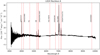 |
Fig. A.1. 1D optical spectrum of the L024A nucleus, extracted over an aperture of ∼1.2 arcsec (∼1.7 kpc at given redshift). Prominent emission lines are marked and labelled. The x-axis represents the wavelength in Angstroms, while the y-axis depicts the flux in units of ergs s−1 cm−2 Å−1. The flattened part of the spectrum between 5500 and 6000 Å is the region where the end of the blue channel overlaps with the beginning of the red channel of MODS. Two additional sections beyond 7500 Åhave been normalised. They coincide with a sky absorption line and a noisy part of the spectrum. |
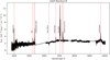 |
Fig. A.2. 1D optical spectrum of the L024B nucleus, extracted over an aperture of ∼1.2 arcsec (∼1.7 kpc at given redshift). Prominent emission lines are marked and labelled. The x-axis represents the wavelength in Angstroms, while the y-axis depicts the flux in units of ergs s−1 cm−2 Å−1. The flattened part of the spectrum between 5500 and 6000 Å is the region, where the end of the blue channel overlaps with the beginning of the red channel of MODS. Two additional sections beyond 7500 Åhave been normalised. They coincide with a sky absorption line and a noisy part of the spectrum. |
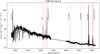 |
Fig. A.3. 1D optical spectrum of the L084A nucleus, extracted over an aperture of ∼1.2 arcsec (∼1.2 kpc at given redshift). Prominent emission lines are marked and labelled. The x-axis represents the wavelength in Angstroms, while the y-axis depicts the flux in units of ergs s−1 cm−2 Å−1. The flattened part of the spectrum between 5500 and 6000 Å is the region where the end of the blue channel overlaps with the beginning of the red channel of MODS. |
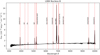 |
Fig. A.4. 1D optical spectrum of the L084B nucleus, extracted over an aperture of ∼1.2 arcsec (∼1.2 kpc at given redshift). Prominent emission lines are marked and labelled. The x-axis represents the wavelength in Angstroms, while the y-axis depicts the flux in units of ergs s−1 cm−2 Å−1. The flattened part of the spectrum between 5500 and 6000 Å is the region, where the end of the blue channel overlaps with the beginning of the red channel of MODS. Two additional sections beyond 7500 Åhave been normalised. They coincide with a sky absorption line and a noisy part of the spectrum. |
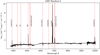 |
Fig. A.5. 1D optical spectrum of the L097A nucleus, extracted over an aperture of ∼1.2 arcsec (∼1.1 kpc at given redshift). Prominent emission lines are marked and labelled. The x-axis represents the wavelength in Angstroms, while the y-axis depicts the flux in units of ergs s−1 cm−2 Å−1. The flattened part of the spectrum between 5500 and 6000 Å is the region where the end of the blue channel overlaps with the beginning of the red channel of MODS. Two additional sections beyond 7500 Åhave been normalised. They coincide with a sky absorption line and a noisy part of the spectrum. |
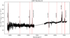 |
Fig. A.6. 1D optical spectrum of the L097B nucleus, extracted over an aperture of ∼1.2 arcsec (∼1.1 kpc at given redshift). Prominent emission lines are marked and labelled. The x-axis represents the wavelength in Angstroms, while the y-axis depicts the flux in units of ergs s−1 cm−2 Å−1. The flattened part of the spectrum between 5500 and 6000 Å is the region where the end of the blue channel overlaps with the beginning of the red channel of MODS. |
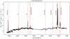 |
Fig. A.7. 1D optical spectrum of the L115A nucleus, extracted over an aperture of ∼1.2 arcsec (∼1.3 kpc at given redshift). Prominent emission lines are marked and labelled. The x-axis represents the wavelength in Angstroms, while the y-axis depicts the flux in units of ergs s−1 cm−2 Å−1. The flattened part of the spectrum between 5500 and 6000 Å is the region where the end of the blue channel overlaps with the beginning of the red channel of MODS. |
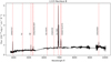 |
Fig. A.8. 1D optical spectrum of the L115B nucleus, extracted over an aperture of ∼1.2 arcsec (∼1.4 kpc at given redshift). Prominent emission lines are marked and labelled. The x-axis represents the wavelength in Angstroms, while the y-axis depicts the flux in units of ergs s−1 cm−2 Å−1. The flattened part of the spectrum between 5500 and 6000 Å is the region where the end of the blue channel overlaps with the beginning of the red channel of MODS. Two additional sections beyond 7500 Åhave been normalised. They coincide with a sky absorption line and a noisy part of the spectrum. |
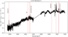 |
Fig. A.9. 1D optical spectrum of the L115C nucleus, extracted over an aperture of ∼1.2 arcsec (∼1.4 kpc at given redshift). Prominent emission lines are marked and labelled. The x-axis represents the wavelength in Angstroms, while the y-axis depicts the flux in units of ergs s−1 cm−2 Å−1. The flattened part of the spectrum between 5500 and 6000 Å is the region where the end of the blue channel overlaps with the beginning of the red channel of MODS. |
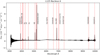 |
Fig. A.10. 1D optical spectrum of the L125A nucleus, extracted over an aperture of ∼1.2 arcsec (∼1.1 kpc at given redshift). Prominent emission lines are marked and named. The x-axis represents the wavelength in Angstroms, while the y-axis depicts the flux in units of ergs s−1 cm−2 Å−1. The flattened part of the spectrum between 5500 and 6000 Å is the region where the end of the blue channel overlaps with the beginning of the red channel of MODS. Two additional sections beyond 7500 Åhave been normalised. They coincide with a sky absorption line and a noisy part of the spectrum. |
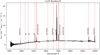 |
Fig. A.11. 1D optical spectrum of the L125B nucleus, extracted over an aperture of ∼1.2 arcsec (∼1.2 kpc at given redshift). Prominent emission lines are marked and labelled. The x-axis represents the wavelength in Angstroms, while the y-axis depicts the flux in units of ergs s−1 cm−2 Å−1. The flattened part of the spectrum between 5500 and 6000 Å is the region where the end of the blue channel overlaps with the beginning of the red channel of MODS. Two additional sections beyond 7500 Åhave been normalised. They coincide with a sky absorption line and a noisy part of the spectrum. |
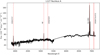 |
Fig. A.12. 1D optical spectrum of the L127A nucleus, extracted over an aperture of ∼1.2 arcsec (∼1.3 kpc at given redshift). Prominent emission lines are marked and labelled. The x-axis represents the wavelength in Angstroms, while the y-axis depicts the flux in units of ergs s−1 cm−2 Å−1. The flattened part of the spectrum between 5500 and 6000 Å is the region where the end of the blue channel overlaps with the beginning of the red channel of MODS. |
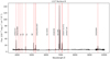 |
Fig. A.13. 1D optical spectrum of the L127B nucleus, extracted over an aperture of ∼1.2 arcsec (∼1.3 kpc at given redshift). Prominent emission lines are marked and labelled. The x-axis represents the wavelength in Angstroms, while the y-axis depicts the flux in units of ergs s−1 cm−2 Å−1. The flattened part of the spectrum between 5500 and 6000 Å is the region where the end of the blue channel overlaps with the beginning of the red channel of MODS. Two additional sections beyond 7500 Åhave been normalised. They coincide with a sky absorption line and a noisy part of the spectrum. |
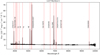 |
Fig. A.14. 1D optical spectrum of the L127C nucleus, extracted over an aperture of ∼1.2 arcsec (∼1.3 kpc at given redshift). Prominent emission lines are marked and labelled. The x-axis represents the wavelength in Angstroms, while the y-axis depicts the flux in units of ergs s−1 cm−2 Å−1. The flattened part of the spectrum between 5500 and 6000 Å is the region where the end of the blue channel overlaps with the beginning of the red channel of MODS. Two additional sections beyond 7500 Åhave been normalised. They coincide with a sky absorption line and a noisy part of the spectrum. |
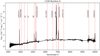 |
Fig. A.15. 1D optical spectrum of the L156A nucleus, extracted over an aperture of ∼1.2 arcsec (∼1.2 kpc at given redshift). Prominent emission lines are marked and labelled. The x-axis represents the wavelength in Angstroms, while the y-axis depicts the flux in units of ergs s−1 cm−2 Å−1. The flattened part of the spectrum between 5500 and 6000 Å is the region where the end of the blue channel overlaps with the beginning of the red channel of MODS. Two additional sections beyond 7500 Åhave been normalised. They coincide with a sky absorption line and a noisy part of the spectrum. |
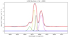 |
Fig. A.16. 1D optical spectrum of the L156A nucleus, showing the Gaussian fitting performed over the Hα+[N II] component. The four narrow components used to perform the fitting are marked by green, yellow, black, and magenta dashed lines, while the best fit is represented by a red line. |
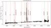 |
Fig. A.17. 1D optical spectrum of the L156B nucleus, extracted over an aperture of ∼1.2 arcsec (∼1.2 kpc at given redshift). Prominent emission lines are marked and labelled. The x-axis represents the wavelength in Angstroms, while the y-axis depicts the flux in units of ergs s−1 cm−2 Å−1. The flattened part of the spectrum between 5500 and 6000 Å is the region where the end of the blue channel overlaps with the beginning of the red channel of MODS. Two additional sections beyond 7500 Åhave been normalised. They coincide with a sky absorption line and a noisy part of the spectrum. |
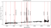 |
Fig. A.18. 1D optical spectrum of the L170A nucleus, extracted over an aperture of ∼1.2 arcsec (∼1.0 kpc at given redshift). Prominent emission lines are marked and labelled. The x-axis represents the wavelength in Angstroms, while the y-axis depicts the flux in units of ergs s−1 cm−2 Å−1. The flattened part of the spectrum between 5500 and 6000 Å is the region where the end of the blue channel overlaps with the beginning of the red channel of MODS. Two additional sections beyond 7500 Åhave been normalised. They coincide with a sky absorption line and a noisy part of the spectrum. |
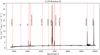 |
Fig. A.19. 1D optical spectrum of the L170B nucleus, extracted over an aperture of ∼1.2 arcsec (∼1.0 kpc at given redshift). Prominent emission lines are marked and labelled. The x-axis represents the wavelength in Angstroms, while the y-axis depicts the flux in units of ergs s−1 cm−2 Å−1. The flattened part of the spectrum between 5500 and 6000 Å is the region where the end of the blue channel overlaps with the beginning of the red channel of MODS. Two additional sections beyond 7500 Åhave been normalised. They coincide with a sky absorption line and a noisy part of the spectrum. |
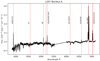 |
Fig. A.20. 1D optical spectrum of the L207A nucleus, extracted over an aperture of ∼1.2 arcsec (∼1.1 kpc at given redshift). Prominent emission lines are marked and labelled. The x-axis represents the wavelength in Angstroms, while the y-axis depicts the flux in units of ergs s−1 cm−2 Å−1. The flattened part of the spectrum between 5500 and 6000 Å is the region where the end of the blue channel overlaps with the beginning of the red channel of MODS. |
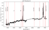 |
Fig. A.21. 1D optical spectrum of the L207B nucleus, extracted over an aperture of ∼1.2 arcsec (∼1.1 kpc at given redshift). Prominent emission lines are marked and labelled. The x-axis represents the wavelength in Angstroms, while the y-axis depicts the flux in units of ergs s−1 cm−2 Å−1. The flattened part of the spectrum between 5500 and 6000 Å is the region where the end of the blue channel overlaps with the beginning of the red channel of MODS. |
All Tables
All Figures
|
Fig. 1. SDSS images of the sample: H011, L024, L084, L097, L115, L125, L127, L156, L170, and L207. The 1 arcsec slit used for the observation is illustrated and the position angle used for each of the observations is marked. Scale is mentioned in each image. North is up and east is to the left. The radio detected galaxy is marked with an ‘r’. |
| In the text | |
|
Fig. 2. 1D optical spectrum of the H011A nucleus, extracted over an aperture of ∼1.2 arcsec (∼1.2 kpc at given redshift). Prominent emission lines are marked and named. The x-axis represents the wavelength in Angstroms, while the y-axis depicts the flux in units of erg s−1 cm−2 Å−1. The flattened part of the spectrum between 5500 and 6000 Å is the region where the end of the blue channel overlaps with the beginning of the red channel of MODS. Two additional sections beyond 7500 Å have been normalised. They coincide with a sky absorption line and a noisy part of the spectrum. |
| In the text | |
|
Fig. 3. 1D optical spectrum of the H011B nucleus, extracted over an aperture of ∼1.2 arcsec (∼1.2 kpc at given redshift). Prominent emission lines are marked and named. The x-axis represents the wavelength in Angstroms, while the y-axis depicts the flux in units of erg s−1 cm−2 Å−1. The flattened part of the spectrum between 5500 and 6000 Å is the region where the end of the blue channel overlaps with the beginning of the red channel of MODS. Two additional sections beyond 7500 Å have been normalised. They coincide with a sky absorption line and a noisy part of the spectrum. |
| In the text | |
|
Fig. 4. SDSS (aperture size ∼3″) contour images of all sources overplotted with FIRST (angular resolution ∼5″ contours). The contour levels are chosen arbitrarily. SDSS contours are in red, while the FIRST contours are indicated with the colour green. North is up and east is to the left. Scale is indicated in each image. |
| In the text | |
|
Fig. 5. Plots of log([O III]λ5007/Hβ) vs. log([N II]λ6583/Hα), log([O III]λ5007/Hβ) vs. log([S II](λ6717+λ6731)/Hα) and log([O III]λ5007/Hβ) vs. log([O I]λ6300/Hα). Each colour marks a particular interacting pair or group. The inverted triangles represent the data points corresponding to nucleus A of a given source, whereas the squares represent the nucleus B, filled circles represent nucleus C, where applicable, and the crosses mark the data point derived from the SDSS spectrum of the source. The data points have been calculated for an aperture of 1 arcsec. The error bars have been derived from the 1σ standard uncertainty values. |
| In the text | |
|
Fig. 6. Plot of log([O III]λ5007/Hβ) vs. log([N II]λ6583/Hα) with a colour map based on the radio spectral indices of the sources derived from radio fluxes of the sources at 1.4 GHz and 4.85 GHz. |
| In the text | |
|
Fig. 7. Plot of log([O III]λ5007/Hβ) vs. log η. Colour bar is defined by the value of the spectral index of the source. |
| In the text | |
|
Fig. 8. Plot of log([O III]λ5007/Hβ) vs. log([N II]λ6583/Hα) with a colour map based on the value of the Eddington ratio of each source. |
| In the text | |
|
Fig. 9. Plot of log([O III]λ5007/Hβ) vs. the radio-loudness parameter (L1.4 GHz/L5100 @@@(LBT)). Green dots represent galaxies with flat radio spectral index (−0.7 ≤ α1.4/4.85 ≤ −0.4), while red dots represent galaxies with inverted radio spectral index (α > −0.4). The vertical blue line represents the median value of the radio-loudness parameter for the non-radio detected galaxies from Table 31 and the magenta arrows indicate that this is the upper limit of the radio-loudness at the log([O III]λ5007/Hβ) values for each of the galaxies. |
| In the text | |
|
Fig. 10. Underlying physical source model of our interpretation. A detailed description is given in Sect. 6.5. |
| In the text | |
|
Fig. 11. Plot of log([O III]λ5007/Hβ) vs. the radio-loudness parameter (L1.4 GHz/L5100 Å (LBT)), as in Fig. 9, but relative contributions of ionising and/or radio detected components in heat colours and black contours. Radio-loudness parameter is estimated using the 5100 Å luminosity from LBT spectra. |
| In the text | |
|
Fig. 12. Scatter plot of the reference radio detected source data presented by Vitale et al. (2015) and Zajaček & Busch (2019). Radio-loudness parameter is estimated using the 5100 Å luminosity from SDSS spectra. |
| In the text | |
|
Fig. 13. Scatter diagram shown in Fig. 12 but collapsed onto the radio-loudness axis (see text in Sect. 6.5). Radio-loudness parameter is estimated using the 5100 Å luminosity from SDSS spectra. |
| In the text | |
|
Fig. 14. Plot of the ionisation ratio of each galactic nuclear region versus the mass of the central SMBH. The crosses and square represent the masses of the non-radio detected galaxies, while the dots represent the radio detected galaxies. Each interacting pair is represented by a specific colour, as described in the legend of the plot. |
| In the text | |
|
Fig. 15. Plot of the radio-loudness parameter of each galactic nuclear region versus the mass of the central SMBH. |
| In the text | |
|
Fig. 16. W1 − W2 versus W2 − W3 colour-colour diagram based on the WISE magnitudes at 3.4 μm, 4.6 μm, and 12 μm. The red dots are the data points for the galaxies in our sample. The dashed black line shows the W1 − W2 > 0.8 criterion proposed by Stern et al. (2012). |
| In the text | |
|
Fig. 17. Plot of log values of the 12 μm luminosity, in erg s−1 units, of the galaxies detected by the WISE W3 band versus the log values of the 1.4 GHz luminosity, in W Hz−1 units, observed in the FIRST survey. The red dots are the data points for the galaxies in our sample. The solid blue line shows the linear regression fit to the data, described by L12 μm = 0.36L1.4 GHz + 35.58. |
| In the text | |
|
Fig. A.1. 1D optical spectrum of the L024A nucleus, extracted over an aperture of ∼1.2 arcsec (∼1.7 kpc at given redshift). Prominent emission lines are marked and labelled. The x-axis represents the wavelength in Angstroms, while the y-axis depicts the flux in units of ergs s−1 cm−2 Å−1. The flattened part of the spectrum between 5500 and 6000 Å is the region where the end of the blue channel overlaps with the beginning of the red channel of MODS. Two additional sections beyond 7500 Åhave been normalised. They coincide with a sky absorption line and a noisy part of the spectrum. |
| In the text | |
|
Fig. A.2. 1D optical spectrum of the L024B nucleus, extracted over an aperture of ∼1.2 arcsec (∼1.7 kpc at given redshift). Prominent emission lines are marked and labelled. The x-axis represents the wavelength in Angstroms, while the y-axis depicts the flux in units of ergs s−1 cm−2 Å−1. The flattened part of the spectrum between 5500 and 6000 Å is the region, where the end of the blue channel overlaps with the beginning of the red channel of MODS. Two additional sections beyond 7500 Åhave been normalised. They coincide with a sky absorption line and a noisy part of the spectrum. |
| In the text | |
|
Fig. A.3. 1D optical spectrum of the L084A nucleus, extracted over an aperture of ∼1.2 arcsec (∼1.2 kpc at given redshift). Prominent emission lines are marked and labelled. The x-axis represents the wavelength in Angstroms, while the y-axis depicts the flux in units of ergs s−1 cm−2 Å−1. The flattened part of the spectrum between 5500 and 6000 Å is the region where the end of the blue channel overlaps with the beginning of the red channel of MODS. |
| In the text | |
|
Fig. A.4. 1D optical spectrum of the L084B nucleus, extracted over an aperture of ∼1.2 arcsec (∼1.2 kpc at given redshift). Prominent emission lines are marked and labelled. The x-axis represents the wavelength in Angstroms, while the y-axis depicts the flux in units of ergs s−1 cm−2 Å−1. The flattened part of the spectrum between 5500 and 6000 Å is the region, where the end of the blue channel overlaps with the beginning of the red channel of MODS. Two additional sections beyond 7500 Åhave been normalised. They coincide with a sky absorption line and a noisy part of the spectrum. |
| In the text | |
|
Fig. A.5. 1D optical spectrum of the L097A nucleus, extracted over an aperture of ∼1.2 arcsec (∼1.1 kpc at given redshift). Prominent emission lines are marked and labelled. The x-axis represents the wavelength in Angstroms, while the y-axis depicts the flux in units of ergs s−1 cm−2 Å−1. The flattened part of the spectrum between 5500 and 6000 Å is the region where the end of the blue channel overlaps with the beginning of the red channel of MODS. Two additional sections beyond 7500 Åhave been normalised. They coincide with a sky absorption line and a noisy part of the spectrum. |
| In the text | |
|
Fig. A.6. 1D optical spectrum of the L097B nucleus, extracted over an aperture of ∼1.2 arcsec (∼1.1 kpc at given redshift). Prominent emission lines are marked and labelled. The x-axis represents the wavelength in Angstroms, while the y-axis depicts the flux in units of ergs s−1 cm−2 Å−1. The flattened part of the spectrum between 5500 and 6000 Å is the region where the end of the blue channel overlaps with the beginning of the red channel of MODS. |
| In the text | |
|
Fig. A.7. 1D optical spectrum of the L115A nucleus, extracted over an aperture of ∼1.2 arcsec (∼1.3 kpc at given redshift). Prominent emission lines are marked and labelled. The x-axis represents the wavelength in Angstroms, while the y-axis depicts the flux in units of ergs s−1 cm−2 Å−1. The flattened part of the spectrum between 5500 and 6000 Å is the region where the end of the blue channel overlaps with the beginning of the red channel of MODS. |
| In the text | |
|
Fig. A.8. 1D optical spectrum of the L115B nucleus, extracted over an aperture of ∼1.2 arcsec (∼1.4 kpc at given redshift). Prominent emission lines are marked and labelled. The x-axis represents the wavelength in Angstroms, while the y-axis depicts the flux in units of ergs s−1 cm−2 Å−1. The flattened part of the spectrum between 5500 and 6000 Å is the region where the end of the blue channel overlaps with the beginning of the red channel of MODS. Two additional sections beyond 7500 Åhave been normalised. They coincide with a sky absorption line and a noisy part of the spectrum. |
| In the text | |
|
Fig. A.9. 1D optical spectrum of the L115C nucleus, extracted over an aperture of ∼1.2 arcsec (∼1.4 kpc at given redshift). Prominent emission lines are marked and labelled. The x-axis represents the wavelength in Angstroms, while the y-axis depicts the flux in units of ergs s−1 cm−2 Å−1. The flattened part of the spectrum between 5500 and 6000 Å is the region where the end of the blue channel overlaps with the beginning of the red channel of MODS. |
| In the text | |
|
Fig. A.10. 1D optical spectrum of the L125A nucleus, extracted over an aperture of ∼1.2 arcsec (∼1.1 kpc at given redshift). Prominent emission lines are marked and named. The x-axis represents the wavelength in Angstroms, while the y-axis depicts the flux in units of ergs s−1 cm−2 Å−1. The flattened part of the spectrum between 5500 and 6000 Å is the region where the end of the blue channel overlaps with the beginning of the red channel of MODS. Two additional sections beyond 7500 Åhave been normalised. They coincide with a sky absorption line and a noisy part of the spectrum. |
| In the text | |
|
Fig. A.11. 1D optical spectrum of the L125B nucleus, extracted over an aperture of ∼1.2 arcsec (∼1.2 kpc at given redshift). Prominent emission lines are marked and labelled. The x-axis represents the wavelength in Angstroms, while the y-axis depicts the flux in units of ergs s−1 cm−2 Å−1. The flattened part of the spectrum between 5500 and 6000 Å is the region where the end of the blue channel overlaps with the beginning of the red channel of MODS. Two additional sections beyond 7500 Åhave been normalised. They coincide with a sky absorption line and a noisy part of the spectrum. |
| In the text | |
|
Fig. A.12. 1D optical spectrum of the L127A nucleus, extracted over an aperture of ∼1.2 arcsec (∼1.3 kpc at given redshift). Prominent emission lines are marked and labelled. The x-axis represents the wavelength in Angstroms, while the y-axis depicts the flux in units of ergs s−1 cm−2 Å−1. The flattened part of the spectrum between 5500 and 6000 Å is the region where the end of the blue channel overlaps with the beginning of the red channel of MODS. |
| In the text | |
|
Fig. A.13. 1D optical spectrum of the L127B nucleus, extracted over an aperture of ∼1.2 arcsec (∼1.3 kpc at given redshift). Prominent emission lines are marked and labelled. The x-axis represents the wavelength in Angstroms, while the y-axis depicts the flux in units of ergs s−1 cm−2 Å−1. The flattened part of the spectrum between 5500 and 6000 Å is the region where the end of the blue channel overlaps with the beginning of the red channel of MODS. Two additional sections beyond 7500 Åhave been normalised. They coincide with a sky absorption line and a noisy part of the spectrum. |
| In the text | |
|
Fig. A.14. 1D optical spectrum of the L127C nucleus, extracted over an aperture of ∼1.2 arcsec (∼1.3 kpc at given redshift). Prominent emission lines are marked and labelled. The x-axis represents the wavelength in Angstroms, while the y-axis depicts the flux in units of ergs s−1 cm−2 Å−1. The flattened part of the spectrum between 5500 and 6000 Å is the region where the end of the blue channel overlaps with the beginning of the red channel of MODS. Two additional sections beyond 7500 Åhave been normalised. They coincide with a sky absorption line and a noisy part of the spectrum. |
| In the text | |
|
Fig. A.15. 1D optical spectrum of the L156A nucleus, extracted over an aperture of ∼1.2 arcsec (∼1.2 kpc at given redshift). Prominent emission lines are marked and labelled. The x-axis represents the wavelength in Angstroms, while the y-axis depicts the flux in units of ergs s−1 cm−2 Å−1. The flattened part of the spectrum between 5500 and 6000 Å is the region where the end of the blue channel overlaps with the beginning of the red channel of MODS. Two additional sections beyond 7500 Åhave been normalised. They coincide with a sky absorption line and a noisy part of the spectrum. |
| In the text | |
|
Fig. A.16. 1D optical spectrum of the L156A nucleus, showing the Gaussian fitting performed over the Hα+[N II] component. The four narrow components used to perform the fitting are marked by green, yellow, black, and magenta dashed lines, while the best fit is represented by a red line. |
| In the text | |
|
Fig. A.17. 1D optical spectrum of the L156B nucleus, extracted over an aperture of ∼1.2 arcsec (∼1.2 kpc at given redshift). Prominent emission lines are marked and labelled. The x-axis represents the wavelength in Angstroms, while the y-axis depicts the flux in units of ergs s−1 cm−2 Å−1. The flattened part of the spectrum between 5500 and 6000 Å is the region where the end of the blue channel overlaps with the beginning of the red channel of MODS. Two additional sections beyond 7500 Åhave been normalised. They coincide with a sky absorption line and a noisy part of the spectrum. |
| In the text | |
|
Fig. A.18. 1D optical spectrum of the L170A nucleus, extracted over an aperture of ∼1.2 arcsec (∼1.0 kpc at given redshift). Prominent emission lines are marked and labelled. The x-axis represents the wavelength in Angstroms, while the y-axis depicts the flux in units of ergs s−1 cm−2 Å−1. The flattened part of the spectrum between 5500 and 6000 Å is the region where the end of the blue channel overlaps with the beginning of the red channel of MODS. Two additional sections beyond 7500 Åhave been normalised. They coincide with a sky absorption line and a noisy part of the spectrum. |
| In the text | |
|
Fig. A.19. 1D optical spectrum of the L170B nucleus, extracted over an aperture of ∼1.2 arcsec (∼1.0 kpc at given redshift). Prominent emission lines are marked and labelled. The x-axis represents the wavelength in Angstroms, while the y-axis depicts the flux in units of ergs s−1 cm−2 Å−1. The flattened part of the spectrum between 5500 and 6000 Å is the region where the end of the blue channel overlaps with the beginning of the red channel of MODS. Two additional sections beyond 7500 Åhave been normalised. They coincide with a sky absorption line and a noisy part of the spectrum. |
| In the text | |
|
Fig. A.20. 1D optical spectrum of the L207A nucleus, extracted over an aperture of ∼1.2 arcsec (∼1.1 kpc at given redshift). Prominent emission lines are marked and labelled. The x-axis represents the wavelength in Angstroms, while the y-axis depicts the flux in units of ergs s−1 cm−2 Å−1. The flattened part of the spectrum between 5500 and 6000 Å is the region where the end of the blue channel overlaps with the beginning of the red channel of MODS. |
| In the text | |
|
Fig. A.21. 1D optical spectrum of the L207B nucleus, extracted over an aperture of ∼1.2 arcsec (∼1.1 kpc at given redshift). Prominent emission lines are marked and labelled. The x-axis represents the wavelength in Angstroms, while the y-axis depicts the flux in units of ergs s−1 cm−2 Å−1. The flattened part of the spectrum between 5500 and 6000 Å is the region where the end of the blue channel overlaps with the beginning of the red channel of MODS. |
| In the text | |
Current usage metrics show cumulative count of Article Views (full-text article views including HTML views, PDF and ePub downloads, according to the available data) and Abstracts Views on Vision4Press platform.
Data correspond to usage on the plateform after 2015. The current usage metrics is available 48-96 hours after online publication and is updated daily on week days.
Initial download of the metrics may take a while.