A Virgo Environmental Survey Tracing Ionised Gas Emission (VESTIGE)

A. Boselli; M. Fossati; J. Roediger; M. Boquien; M. Fumagalli; M. Balogh; S. Boissier; J. Braine; L. Ciesla; P. Côté; J.C. Cuillandre; L. Ferrarese; G. Gavazzi; S. Gwyn; Junais Junais; G. Hensler; A. Longobardi; M. Sun

doi:10.1051/0004-6361/202244267

Home

All issues

Volume 669 (January 2023)

A&A, 669 (2023) A73

Full HTML

Open Access

Issue		A&A Volume 669, January 2023


Article Number		A73
Number of page(s)		27
Section		Extragalactic astronomy
DOI		https://doi.org/10.1051/0004-6361/202244267
Published online		11 January 2023

A&A 669, A73 (2023)

XIV. Main-sequence relation in a rich environment down to M_star ≃ 10⁶ M_⊙^⋆

A. Boselli¹^,⋆⋆, M. Fossati², J. Roediger³, M. Boquien⁴, M. Fumagalli², M. Balogh⁵, S. Boissier¹, J. Braine⁶, L. Ciesla¹, P. Côté³, J.C. Cuillandre⁷, L. Ferrarese³, G. Gavazzi², S. Gwyn³, Junais⁸, G. Hensler⁹, A. Longobardi² and M. Sun¹⁰

¹ Aix-Marseille Univ., CNRS, CNES, LAM, Marseille, France
e-mail: alessandro.boselli@lam.fr
² Universitá di Milano-Bicocca, Piazza della Scienza 3, 20100 Milano, Italy
³ National Research Council of Canada, Herzberg Astronomy and Astrophysics, 5071 West Saanich Road, Victoria, BC V9E 2E7, Canada
⁴ Centro de Astronomiá (CITEVA), Universidad de Antofagasta, Avenida Angamos 601, Antofagasta, Chile
⁵ Waterloo Centre for Astrophysics, University of Waterloo, Waterloo, Ontario N2L3G1, Canada
⁶ Laboratoire d’Astrophysique de Bordeaux, Univ. Bordeaux, CNRS, B18N, allée Geoffroy Saint-Hilaire, 33615 Pessac, France
⁷ AIM, CEA, CNRS, Université Paris-Saclay, Université Paris-Diderot, Sorbonne Paris-Cité, Observatoire de Paris, PSL University, 91191 Gif-sur-Yvette Cedex, France
⁸ National Centre for Nuclear Research, Pasteura 7, 02-093 Warsaw, Poland
⁹ Department of Astrophysics, University of Vienna, Türkenschanzstrasse 17, 1180 Vienna, Austria
¹⁰ Department of Physics & Astronomy, University of Alabama in Huntsville, 3001 Sparkman Drive, Huntsville, AL 35899, USA

Received: 14 June 2022
Accepted: 29 October 2022

Abstract

Using a compilation of Hα fluxes for 384 star-forming galaxies detected during the Virgo Environmental Survey Tracing Ionised Gas Emission (VESTIGE), we study several important scaling relations linking the star formation rate, specific star formation rate, stellar mass, stellar mass surface density, and atomic gas depletion timescale for a complete sample of galaxies in a rich environment. The extraordinary sensitivity of the narrow-band imaging data allows us to sample the whole dynamic range of the Hα luminosity function, from massive galaxies (M_star ≃ 10¹¹ M_⊙) to dwarf systems (M_star ≃ 10⁶ M_⊙), where the ionised gas emission is due to the emission of single O-early B stars. This extends previous works to a dynamic range in stellar mass and star formation rate (10⁻⁴ ≲ SFR ≲ 10 M_⊙ yr⁻¹) that has never been explored so far. The main-sequence relation derived for all star-forming galaxies within one virial radius of the Virgo cluster has a slope comparable to that observed in other nearby samples of isolated objects, but its dispersion is about three times larger (∼1 dex). The dispersion is tightly connected to the available amount of HI gas, with gas-poor systems located far below objects of similar stellar mass, but with a normal HI content. When measured on unperturbed galaxies with a normal HI gas content (HI-def ≤ 0.4), the relation has a slope a = 0.92 ± 0.06, an intercept b = −1.57 ± 0.06 (at a pivot point of log M_star = 8.451 M_⊙), and a scatter σ ≃ 0.40, and it has a constant slope in the stellar mass range 10⁶ ≲ M_star ≲ 3 × 10¹¹ M_⊙. The specific star formation rate of HI-poor galaxies is significantly lower than that of HI-rich systems of similar stellar mass, while their atomic gas consumption timescale τ_HI is fairly similar, in particular, for objects of stellar mass 10⁷ ≲ M_star ≲ 10⁹ M_⊙. We compare these observational results to the prediction of models expressly tuned to reproduce the effects induced by the interaction of galaxies with their surrounding environment. The observed scatter in the main-sequence relation can be reproduced only after a violent and active stripping process such as ram-pressure stripping that removes gas from the disc (outer parts first) and quenches star formation on short (< 1 Gyr) timescales. This rules out milder processes such as starvation. This interpretation is also consistent with the position of galaxies of different star formation activity and gas content within the phase-space diagram. We also show that the star-forming regions that formed in the stripped material outside perturbed galaxies are located well above the main-sequence relation drawn by unperturbed systems. These extraplanar HII regions, which might be at the origin of ultra-compact dwarf galaxies (UCDs) and other compact sources typical in rich environments, are living a starburst phase lasting only ≲50 Myr. They later become quiescent systems.

Key words: galaxies: star formation / galaxies: ISM / galaxies: evolution / galaxies: interactions / galaxies: clusters: general / galaxies: clusters: individual: Virgo

^⋆

Based on observations obtained with MegaPrime/MegaCam, a joint project of CFHT and CEA/DAPNIA, at the Canada-French-Hawaii Telescope (CFHT) which is operated by the National Research Council (NRC) of Canada, the Institut National des Sciences de l’Univers of the Centre National de la Recherche Scientifique (CNRS) of France and the University of Hawaii.

^⋆⋆

Scientific associate INAF at the Osservatorio Astronomico di Brera, Italy.

© The Authors 2023

Open Access article, published by EDP Sciences, under the terms of the Creative Commons Attribution License (https://creativecommons.org/licenses/by/4.0), which permits unrestricted use, distribution, and reproduction in any medium, provided the original work is properly cited.

This article is published in open access under the Subscribe-to-Open model. Subscribe to A&A to support open access publication.

1. Introduction

The physical, structural, and kinematical properties of galaxies are tightly connected via several scaling relations between important parameters such as stellar masses, diameters, luminosities, and rotational velocities that can be accurately measured using multifrequency observations. These important relations are often studied in the literature since they retain the imprint of different processes that shaped galaxy formation and evolution. For this reason, they are often used to constrain free parameters in galaxy models, either semi-analytic or in full cosmological simulations. Among these scaling relations, the so-called main-sequence relation, which links the star formation activity of galaxies to their stellar mass (e.g., Brinchmann et al. 2004; Daddi et al. 2007; Elbaz et al. 2007; Noeske et al. 2007; Speagle et al. 2014), is critically important. Although its origin is driven by the range in scales of the galaxy formation process (“bigger galaxies have more of everything”; Kennicutt 1990), the main-sequence relation has been the subject of hundreds of dedicated works because it is tightly connected to the star formation history of galaxies. The evidence that most star-forming galaxies populate a tight sequence in star formation rate (SFR) versus stellar mass for more than 12 Gyr of cosmic time (e.g., Whitaker et al. 2014; Schreiber et al. 2015) places strong constraints on the regulation of the star formation process in galaxies. In the so-called bathtub models (e.g., Bouché et al. 2010; Lilly et al. 2013), the balance of gas inflows, star formation, and outflows due to stellar feedback naturally explain the presence of a star-forming main sequence with a small intrinsic scatter of ∼0.3 dex (Noeske et al. 2007; Whitaker et al. 2012). As a result, particular attention has been given to the study of the main-sequence parameters in different stellar mass regimes, including the origin of the scatter and its possible evolution with redshift (e.g., Rodighiero et al. 2011; Whitaker et al. 2012, 2014; Ilbert et al. 2013; Speagle et al. 2014; Gavazzi et al. 2015; Tasca et al. 2015; Schreiber et al. 2015; Erfanianfar et al. 2016; Pearson et al. 2018; Popesso et al. 2019, 2022). For instance, it has been shown that above a given stellar mass, the slope of the relation decreases, indicating a partial quenching of the activity of star formation attributed either to AGN feedback (Bouché et al. 2010; Lilly et al. 2013) or to a secular evolution due to the presence of prominent bulges or bars (e.g., Gavazzi et al. 2015; Erfanianfar et al. 2016).

The main-sequence relation has been also used to study the effects of the environment on galaxy evolution. It is now well established that galaxies inhabiting rich environments undergo a different evolution than their counterparts in the field. High-density regions are characterised by a dominant quiescent population (morphology segregation effect; Dressler 1980; Whitmore et al. 1993), and their spiral population is generally composed of gas-poor objects (Haynes & Giovanelli 1984; Cayatte et al. 1990; Solanes et al. 2001; Gavazzi et al. 2005, 2006b, 2013; Boselli et al. 2014b,c) with a reduced star formation activity (Gavazzi et al. 1998, 2002, 2006a, 2010, 2013; Boselli et al. 2015). Different physical mechanisms have been proposed in the literature to explain these differences, including galaxy harassment (e.g., Moore et al. 1998), starvation (e.g., Larson et al. 1980; Balogh et al. 2000) and ram-pressure stripping (Gunn & Gott 1972; Boselli et al. 2022a), as reviewed in Boselli & Gavazzi (2006, 2014). The identification of the dominant mechanism as a function of galaxy and host halo mass, however, is still hotly debated. Multifrequency observations of large statistical samples in the nearby Universe or of selected representative objects in nearby clusters indicate that ram-pressure stripping is the most important phenomenon for the gas removal and for the following quenching of the star formation activity (e.g., Boselli et al. 2022a). Conversely, observations of large statistical samples compared to the prediction of cosmological simulations suggest that other milder mechanisms such as starvation are at the origin of the observed suppression of the star formation activity in galaxies inhabiting high-density regions (McGee et al. 2009; Wolf et al. 2009; von der Linden et al. 2010; De Lucia et al. 2012; Wheeler et al. 2014; Taranu et al. 2014; Haines et al. 2015).

The study of the main-sequence relation can be of great help in understanding the effects of the environment on the activity of star formation in cluster galaxies. For instance, the scatter in the relation can be modulated by an increased or a reduced activity in perturbed systems. The main-sequence relation in rich environments has been studied in detail in local (e.g., Tyler et al. 2013, 2014; Boselli et al. 2015, 2022a; Paccagnella et al. 2016; Vulcani et al. 2018) and more distant samples (e.g., Vulcani et al. 2010; Tran et al. 2010, 2017; Koyama et al. 2013; Zeimann et al. 2013; Lin et al. 2014; Erfanianfar et al. 2016; Old et al. 2020; Nantais et al. 2020), and it was compared to the predictions of hydrodynamic simulations (e.g., Sparre et al. 2015; Wang et al. 2018; Donnari et al. 2019; Matthee & Schaye 2019). The results obtained so far often give inconsistent results. Some of them suggest that at intermediate redshift (z ∼ 0.4), the activity of star formation in cluster galaxies is higher (e.g., Koyama et al. 2013) than in field objects. Others indicate galaxies with a reduced star formation activity (e.g., Vulcani et al. 2010; Lin et al. 2014; Erfanianfar et al. 2016). Systematic differences in the results are also present in local studies, some of which indicate a higher activity in ram-pressure-stripped galaxies (e.g., Vulcani et al. 2018), other rather suggesting a comparable (e.g., Tyler et al. 2013, 2014) or lower activity (e.g., Boselli et al. 2015; Paccagnella et al. 2016). Furthermore, whenever the observational evidence was consistent, the results were explained with different perturbing mechanisms, such as a slow quenching process in galaxies with a lower star formation activity by Paccagnella et al. (2016) or a rather rapid quenching due to a ram-pressure-stripping episode (e.g., Boselli et al. 2014b,c, 2015, 2016a).

The difference in these observational results and/or in their interpretation might be strongly related to observational biases, to selection criteria, or to the limited dynamic range in the analysed samples. The Virgo Environmental Survey Tracing Ionised Gas Emission (VESTIGE; Boselli et al. 2018a) is a deep Hα narrow-band imaging survey of the Virgo cluster. The Hα emission line is a hydrogen recombination line produced in the gas ionised by young (≲10 Myr) and massive (M_star ≥ 10 M_⊙) O and early-B stars, and is thus considered as the most direct tracer of recent star formation activity in galaxies (e.g., Kennicutt 1998a,b; Boselli et al. 2009). Through its untargeted nature, VESTIGE provides us with a unique sample of galaxies that is perfectly defined for a complete census of the star formation activity in a rich nearby cluster of galaxies. Designed to cover the whole Virgo cluster up to its virial radius, the survey is sufficiently deep to detect all Hα emitting sources brighter than L(Hα) 10^36.5 erg s⁻¹, corresponding to star formation rates of SFR ≥ 2 × 10⁻⁵ M_⊙ yr⁻¹ and stellar masses M_star ≥ 10⁶ M_⊙, which are values that are never reached in other nearby or high-redshift clusters. Furthermore, the proximity of the cluster (16.5 Mpc; Mei et al. 2007) and the availability of multifrequency data covering the whole electromagnetic spectrum obtained with other untargeted surveys of comparable sensitivity (e.g., UV with GUViCS; Boselli et al. 2011; visible with NGVS; Ferrarese et al. 2012; far-IR with HeViCS; Davies et al. 2010; HI with ALFALFA¹; Giovanelli et al. 2005) are crucial for a coherent study aimed at identifing the dominant perturbing mechanism that is at the origin of galaxy transformation in a rich environment. The galaxies analysed in this work were detected during the VESTIGE survey and are used to reconstruct the main-sequence relation and a few other scaling relations of galaxies within the Virgo cluster. The narrow-band imaging observations are described in Sect. 2, along with the multifrequency observations used in the analysis. In Sect. 3 we describe how the data were corrected for [NII] contamination and dust attenuation, and how they were transformed into star formation rates. The most important scaling relations requiring an accurate determination of the star formation activity of galaxies including the main-sequence relation are described, analysed, and compared to the predictions of tuned models in Sects. 4 and 5. The discussion and conclusion are presented in Sects. 6 and 7.

2. Observations and data reduction

2.1. VESTIGE narrow-band imaging

The data analysed in this work were gathered during the VESTIGE survey, which is an untargeted Hα narrow-band (NB) imaging survey covering the Virgo cluster up to its virial radius (104°²). The observations were carried out using MegaCam at the CFHT in the NB filter MP9603 (λ_c = 6591 Å; Δλ = 106 Å). At the redshift of the galaxies (−300 ≤ v_hel ≤ 3000 km s⁻¹), the filter includes the emission of the Balmer Hα line (λ = 6563 Å) and of the two [NII] lines (λ = 6548, 6583 Å)². The survey is now complete to ∼76%, with an integration time of 2 h in the NB filter and 12 min in the broad-band r filter, which is necessary to subtract the stellar continuum emission. The full depth of the survey has been realised over most of the cluster, with some shorter exposures at the periphery. The observing strategy, which was fully described in Boselli et al. (2018a), consists of mapping the full cluster with MegaCam. This is a wide-field detector composed of 40 CCDs with a pixel scale of 0.187 arcsec pixel⁻¹. The full cluster was mapped following a specific observing sequence optimised for the determination of the sky background necessary for the detection of extended features with low surface brightness. For this purpose, the images were gathered using a large dithering (15 arcmin in RA and 20 arcmin in Dec), which is necessary to minimise any possible contribution of unwanted reflections of bright stars in the construction of the sky flat fields. The observations were obtained under excellent seeing conditions (θ = 0.76″ ± 0.07″) for both the narrow- and broad-band images. The sensitivity of the survey is f(Hα)≃4 × 10⁻¹⁷ erg s⁻¹ cm⁻² (5σ) for point sources and Σ(Hα)≃2 × 10⁻¹⁸ erg s⁻¹ cm⁻² arcsec⁻² (1σ after smoothing the data to a resolution of ∼3″) for extended sources.

Consistently with previous works, the images were reduced using Elixir-LSB (Ferrarese et al. 2012), which is a data reduction pipeline that was expressly designed to detect extended low surface brightness structures such as those expected in interacting systems. The data were photometrically calibrated and corrected for astrometry using the standard MegaCam procedures described in Gwyn (2008), with a typical photometric accuracy in the two bands of ≲0.02–0.03 mag.

The subtraction of the stellar continuum emission was secured as described in Boselli et al. (2019). This process is particularly critical in the centre of early-type galaxies, where the emission in the NB filter is highly dominated by that of the stars. The contribution of the stellar continuum within the NB filter was estimated using the r-band frame combined with a g − r colour to take any possible variation of the spectral energy distribution within the broad-band image into account. For this purpose, we used the g-band images gathered at the CFHT under similar conditions during the NGVS survey (Ferrarese et al. 2012).

2.2. Galaxy identification

The Hα emitting sources were identified after visual inspection of all the continuum-subtracted images as follows. We first searched for any line-emitting source associated with all of the 2096 galaxies included in the Virgo Cluster Catalogue (VCC; Binggeli et al. 1985), and we identified 307 galaxies with emission at the redshift of the cluster. Given the tight relation between cold gas and star formation activity, we then searched for possible counterparts to the HI detected sources in the ALFALFA survey (Giovanelli et al. 2005). This is a HI blind survey carried out with the Arecibo radio telescope and covers the whole Virgo cluster region mapped by VESTIGE. This HI survey, which has a typical sensitivity of rms = 2.3 mJy at 10 km s⁻¹ spectral resolution and 3.2′ angular resolution, is able to detect galaxies at the distance of the Virgo cluster with HI masses of M_HI ≃ 10^7.5 M_⊙. For this purpose, we used the ALFALFA catalogue of Haynes et al. (2018), and included only those Hα sources with a HI redshift ≤ 3000 km s⁻¹ (37 objects). We then searched for any possible counterpart of the 3689 galaxies identified in the NGVS survey as Virgo cluster members by the use of different scaling relations, as extensively described in Ferrarese et al. (2012, 2020; Lim et al. 2020; 31 objects). Four extra bright galaxies with clear Hα emission located outside the NGVS and VCC footprint were included. Finally, we visually inspected all the Hα continuum-subtracted images gathered during the VESTIGE survey and identified a few other extended emitting sources not included in the previous catalogues (five objects). To avoid any possible contamination of background line emitters, we excluded all sources without any clear structured and extended emission typical of compact nearby dwarf systems, such as multiple HII regions and extended filaments. We recall that the trasmissivity curve of the NB filter perfectly matches that of line emitters in the Virgo cluster, thus the detection of any line-emitting source with these properties grants membership to the cluster. The final sample of Hα emitting galaxies analysed in this work thus includes 384 Virgo cluster objects. Figure 1 shows the stellar mass distribution of the Hα detected objects compared to that of the VCC and NGVS galaxies identified as Virgo cluster members. Most of the morphologically classified late-type galaxies included in the VCC (spirals, Magellanic irregulars, and blue compact dwarfs (BCDs)) are detected in Hα, with a few early-type systems mainly characterised by a nuclear or circumnuclear star formation activity (e.g., Boselli et al. 2008a, 2022b). The large majority of the Virgo cluster members that remain undetected by VESTIGE are early-type systems (E, S0, dE, and dS0). Since the sensitivity of the survey is able to detect a single early-B star at the distance of the cluster (see Sect. 3.4), Fig. 1 indicates that the galaxies forming massive, ionising stars are only ∼10% of the Virgo cluster population. For this reason, censoring is not expected to significantly affect the results.

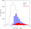Fig. 1.

Stellar mass distribution of the Hα detected galaxies (filled red histogram), of the VCC (hatched blue histogram) and of the NGVS galaxies (empty black histogram) classified as Virgo cluster members. Stellar masses are derived as described in Sect. 3.1.

2.3. Flux extraction

The Hα total flux of each source was computed using the same procedure as in previous VESTIGE works, which was described in Fossati et al. (2018) and Boselli et al. (2018b,c). Fluxes and uncertainties were derived by measuring both the galaxy emission and the sky background within the same elliptical aperture randomly located on the sky after masking other contaminating sources. The elliptical apertures were optimised to encompass the total Hα emission on the galaxy disc and at the same time minimise the sky contribution within the aperture. This was not always optimal in a few low surface brightness extended galaxies in which the Hα emission was dominated by a few HII regions that are located at different edges of the disc. Furthermore, to minimise possible effects due to large-scale residual gradients in the continuum-subtracted frames, the sky background was measured 1000 times within about five times the diameter of the target. The uncertainties on the fluxes were obtained as the quadratic sum of the uncertainties on the flux counts and the uncertainties on the background (rms of the bootstrap iterations). The uncertainties on the flux counts were derived assuming a Poissonian distribution for the source photo-electrons. In a few objects, the resulting signal-to-noise ratio (S/N) is very low, close to 1. Despite their weak emission, however, these are bona fide detections because all consist of several HII regions with a correlated diffuse signal. As mentioned above, their low S/N arises because the few HII regions in these galaxies are located at large distances within the stellar disc, thus the large uncertainty on the measurement is principally due to the uncertain measure of the sky in the large aperture adopted for the flux extraction.

2.4. Multifrequency data

The analysis presented in this work was made possible by the large number of multifrequency data available for the Virgo cluster region (see Table 1). Spectroscopic data in the optical domain are necessary to correct the fluxes obtained in the NB continuum-subtracted images for [NII] contamination and dust attenuation. Integrated spectroscopy gathered by drifting the slit of the spectrograph over the stellar disc is available for the brightest galaxies included in the Herschel Reference Survey (HRS; Boselli et al. 2013), and for several other cluster members in Gavazzi et al. (2004). Optical spectroscopy of the nuclear regions is also available from the Sloan Digital Sky Survey (SDSS). A few objects also have dedicated Focal Reducer and low dispersion Spectrographg (FORS) and Multi Unit Spectroscopic Explorer (MUSE) observations at the VLT of excellent quality (e.g., Fossati et al. 2018; Boselli et al. 2018c, 2021, 2022b).

Table 1.

Multifrequency data.

The dust attenuation of the Hα fluxes can also be corrected for using mid-IR data. For this purpose, we used WISE (Wright et al. 2010) 22 μm fluxes obtained for the brightest galaxies included in the HRS by Ciesla et al. (2014), or for the remaining Virgo cluster members by Boselli et al. (2014c). For a few galaxies that were not included in these catalogues, we extracted Wide-field Infrared Survey Explorer (WISE) 22 μm fluxes from the images as described in Boselli et al. (2014c).

We also used optical images obtained during the NGVS survey (Ferrarese et al. 2012) to secure an accurate subtraction of the stellar continuum emission, to optically identify the Hα emitting sources, and to determine their total stellar mass. Total magnitudes in the u, g, i, z photometric bands were measured following one of two approaches: fitting elliptical isophotes with a bespoke code based on IRAF/ELLIPSE, or fitting 2D Sérsic models with GALFIT³ (see Ferrarese et al. 2020). For galaxies with a photographic magnitude in the VCC calatogue B_VCC < 16 mag, we drew growth curves from IRAF/ELLIPSE, and measured fluxes within the first isophote at which the g-band growth curve flattens. For all other galaxies, we used the total fluxes (integrated to infinity) of the best-fit model found by GALFIT. Errors in the integrated fluxes were estimated by summing the per-pixel contributions from Poisson noise of the source and sky, and read noise, while enforcing lower limits equal to the precision of the NGVS photometric calibration.

Finally, we used different sets of HI data to identify the Hα emitting source (ALFALFA; Giovanelli et al. 2005; Haynes et al. 2018) and to determine the HI-deficiency parameter. This parameter is generally used in the literature to identify galaxies with a low atomic gas content that is probably due to a recent interaction with their surrounding cluster environment (e.g., Cortese et al. 2021; Boselli et al. 2022a). This parameter is defined as the difference between the expected and the observed HI gas mass of each single galaxy on a logarithmic scale (Haynes & Giovanelli 1984), where the expected atomic gas mass is the mean HI mass of a galaxy of a given optical size and morphological type determined in a complete reference sample of isolated objects. For this purpose, we used here the recent calibration of Cattorini et al. (2022), which is based on a sample of ∼8000 galaxies in the nearby universe. We remark that this calibration is optimised for massive and dwarf systems; dwarf systems were generally undersampled in previous determinations (e.g., Haynes & Giovanelli 1984; Solanes et al. 1996; Boselli & Gavazzi 2009). The calibration is highly uncertain for early-type galaxies, where the atomic gas content does not necessary follow well-defined scaling relations (e.g., Serra et al. 2012). Throughout this work, we consider as unperturbed objects those with a HI-deficiency parameter HI-def ≤ 0.4, which is the typical dispersion in the scaling relation used to calibrate this parameter (e.g., Haynes & Giovanelli 1984; Cattorini et al. 2022). To determine the HI-deficiency parameter, we used in first priority the HI data collected in the GoldMine database (Gavazzi et al. 2003), which are generally gathered through deep pointed observations mainly with the Arecibo radio telescope (typical rms ≲ 1 mJy). Otherwise, we used the ALFALFA data (Haynes et al. 2018), which cover the entire cluster region at a homogeneous sensitivity and have been also used to derive stringent upper limits to the total HI mass and lower limits to the HI-deficiency parameter of Hα detected sources without any available HI pointed observation. Upper limits in the HI mass (in solar units) were derived using the relation (e.g., Boselli 2011)

$\begin{matrix} M_{{HI}_{ul}} = 2.356 \times 10^{5} d^{2} 2 \times rms \sqrt{200 \times δ V_{HI} \times \sin (i)}, \end{matrix}$ $\begin{aligned} {M_{\mathrm{HI}_{\rm ul}} = 2.356 \times 10^{5} d^2 \ {2 \times \mathrm{rms}} \sqrt{200 \times \delta V_{\rm HI} \times \mathrm{sin}(i)}} ,\end{aligned}$ (1)

where d is the distance of the galaxy (in Mpc; see Sect. 3.4), rms is the rms of the HI data (in Jy; here assumed to be rms = 2.3 mJy) measured for a spectral resolution δV_HI (10 km s⁻¹), and i is the inclination of the galaxy on the plane of the sky. Since all the HI undetected galaxies are dwarf systems, we assumed that their rotational velocity is 200 km s⁻¹. The determination of the HI-deficiency parameter requires an estimate of the B-band 25 mag arcsec⁻² isophotal diameter D₂₅(B). Whenever this value was not available in the VCC, we derived it using the effective radius R_e(g) available in the NGVS data catalogue measured as described in Ferrarese et al. (2020). Effective radii were transformed into B-band isophotal diameters through the relation

$\begin{matrix} D_{25} (B) [arcmin] = \frac{R_{e} (g) [arcsec]}{15.043}, \end{matrix}$ $\begin{aligned} {D_{25}(B) \ \ \mathrm {[arcmin]}} = \frac{R_{\rm e}(g) \ \ \mathrm {[arcsec]}}{15.043} ,\end{aligned}$ (2)

which we calibrated on a large sample of galaxies for which both sets of data are available. The inclination of each single galaxy i was derived as described in Haynes & Giovanelli (1984) with the axial ratios given in the VCC whenever available, or from the NGVS catalogue for the remaining cases. Although important in the star formation process, we did not consider the molecular gas phase because of an evident lack of data. Data are available only for the most massive ∼15% galaxies of the sample (Boselli et al. 2014c; Brown et al. 2021).

As indicated in Table 1, the photometric and spectroscopic coverage of the sample is optimal in the optical, UV, and HI bands, but it is limited to ∼45–50% in the infrared bands (∼70–80% when stringent upper limits are included). Because of the all-sky coverage of the WISE survey, the undetected galaxies are all very faint sources at 22 μm, while those lacking are too faint to give stringent upper limits for the spectral energy distribution (SED) fitting analysis. Those lacking in the five Herschel bands are located outside the footprint of the HeViCS survey (Davies et al. 2010).

3. Derived parameters

3.1. Stellar masses

To estimate the stellar mass, we modelled the SED of our sample with the latest version of the Code Investigating GALaxy Emission (CIGALE; Boquien et al. 2019). To do this, we considered a flexible star formation history (SFH) consisting of a delayed SFH (∝t × exp(−t/τ)), with a recent burst or quench (module sfhdelayedbq). We set the age of all the galaxies to common value of 13 Gyr. The e-folding time free, sampling 10 values from 1 Myr to 8 Gyr. The most recent variation of the SFH was set to have occurred between 10 Myr and 1 Gyr ago, sampling nine values. This strength, which is defined as the ratio of the SFR after and before the beginning of the burst, ranges from 0 (complete quench) to 10 (strong burst), with a sampling of 10 values. This particular shape of the SFH was chosen to take into account the possible abrupt variations in star formation activity observed in perturbed cluster galaxies (e.g., Boselli et al. 2016b, 2021; Fossati et al. 2018). The stellar spectrum was computed from the Bruzual & Charlot (2003) single stellar populations with a Chabrier (2003) initial mass function (IMF) with a fixed metallicity Z = 0.02. We included the nebular emission, with a gas metallicity following that of the stars, an ionisation parameter log U = −3, and an electron density n_e = 100 cm⁻³. The emission was attenuated with a modified starburst law (Calzetti et al. 1994, 2000), with a line reddening covering 16 values from 0.005 mag to 0.6 mag. The differential reddening was allowed to vary, with the continuum having a lower reddening by a factor 0.25, 0.5, or 0.75. An optional bump was included with a strength up to that of the Milky Way. For more flexibility, the attenuation curve slope was multiplied by a power law of index δ ranging from 0 (bona fide starburst) to −1 (steeper than the Large Magellanic Cloud (LMC)). Finally, the dust emission was modelled with the Dale et al. (2014) dust template, with α taking 8 values from 0.5 to 4. Overall, we computed a grid of 15.206.400 models.

All the models were fitted to the observations using the GALEX far- (FUV) and near-ultraviolet (NUV) bands, Megacam u, g, i, z (for the galaxies VCC 322 and VCC 331, which do not have available NGVS data, we used the SDSS magnitudes given in the Extended Virgo Cluster Catalogue (EVCC; Kim et al. 2014), WISE 22 μm, and Herschel at 100, 160, 250, 350, and 500 μm. Upper limits were handled by computing the χ² through Eq. (15) from Boquien et al. (2019). The stellar mass and the related uncertainties were estimated from the likelihood-weighted mean and standard deviation from the model. The mean uncertainty on the stellar mass given by the SED fitting analysis is 0.07 dex, and it increases to 0.08 dex in the low-mass systems (M_star < 10⁸ M_⊙), for which the photometric coverage of the sample is less complete. The uncertainty on the stellar mass, however, is always < 0.15 dex, and is larger than 0.1 dex in only 12% of the sample. These low uncertainties arise because (i) an infrared flux or stringent upper limit necessary to constrain the dust attenuation is available for > 80% of the sample, and (ii) galaxies without IR data are the lowest-mass systems of the sample, where dust attenuation, if present, is minimum (see Sect. 3.3 and Fig. 2). To further confirm the accuracy of these values, we compared the stellar masses derived using the CIGALE SED fitting code with those derived for the whole NGVS sample using PROSPECTOR, an SED fitting code based on the flexible stellar population synthesis model suite of Conroy et al. (2009), using similar parameters for the IMF and the star formation history of the sample galaxies, but using only the four NGVS photometric bands (ugiz) and excluding any dust attenuation correction (Roediger, priv. comm.). The agreement between the two estimates is remarkable, with a mean ratio of 0.05 dex and a dispersion of ∼0.13 dex. This difference is similar to the one generally obtained when stellar mass estimates derived using different codes are compared (e.g., Conroy 2013) that depend on the assumed star formation histories, population synthesis codes, dust attenuation laws, and so on. We estimate that the uncertainty on M_star is somewhere in between the uncertainty given by the CIGALE SED fitting code and the one derived by adding in quadrature an additional source of uncertainty due to the adopted model (e.g. assumed IMF, stellar population synthesis model, SFH, metallicity, and SED fitting code) that we define as modelling uncertainty and assumed to be 0.1 dex (Conroy et al. 2009; Hunt et al. 2019). The resulting mean uncertainty on M_star is thus 0.07 ≲ σ(log M_star)≲0.14 dex.

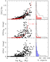Fig. 2.

Correction for [NII] contamination. Left panels: relation between the [NII]λ6548 + 6583 Å/Hα line ratio (upper panel), the dust attenuation measured using the Balmer decrement A(Hα)_BD (middle panel), and the dust attenuation A(Hα) derived by averaging the Balmer decrement and the far-infrared determinations (see Sect. 3.3; lower panel) and the stellar mass of the selected galaxies. The long-dashed red lines indicate the mean relations derived in this work. Right panels: [NII]λ6548 + 6583 Å/Hα, A(Hα)_BD, and A(Hα) distributions. The hatched red and blue histograms give the distribution of [NII]λ6548 + 6583 Å/Hα, A(Hα)_BD, and A(Hα) derived from the mean scaling relations given in the text and adopted in the Hα flux correction for galaxies without any spectroscopic data.

We also derived stellar mass surface densities defined as in Boselli et al. (2014a),

$\begin{matrix} μ_{star} [M_{⊙} {kpc}^{- 2}] = \frac{M_{star}}{2 π R_{e} {(i)}^{2}}, \end{matrix}$ $\begin{aligned} {\mu _{\rm star} \ \ [M_{\odot }\,\mathrm {kpc^{-2}}] = {\frac{M_{\rm star}}{2\pi R_{\rm e}(i)^2}} } ,\end{aligned}$ (3)

where R_e(i) is the effective radius in the i-band in kpc (the factor 2 at the denominator of Eq. (3) is adopted here since R_e(i) is an effective radius, the radius including half of the total i-band light, thus presumably also ∼50% of the total stellar mass). This quantity is available for 216 objects of the sample. For galaxies without a growth curve in the NGVS catalogue (168 objects), R_e(i) was derived from the B-band isophotal diameter using the relation

$\begin{matrix} R_{e} (i) [arcsec] = 16.189 \times D_{25} (B) [arcmin] \end{matrix}$ $\begin{aligned} {R_{\rm e}(i) \ \ \mathrm {[arcsec]} }= {16.189 \times D_{25}(B) \ \ \mathrm {[arcmin]}} \end{aligned}$ (4)

measured on a large sample of galaxies for which both sets of data are available.

3.2. [NII] contamination

The Hα fluxes extracted from the images can be converted into SFRs when they are corrected for the contamination of the [NII] emission lines in the NB filter and for dust attenuation. The contribution of the [NII] lines to the total line emission of each source within the NB filter was measured, in order of priority, using targeted MUSE or the long-slit high-quality observations published in Boselli et al. (2018c, 2021, 2022b) and Fossati et al. (2018; 12 galaxies), long-slit integrated spectra of Boselli et al. (2013) and published in Boselli et al. (2015; 72 objects), similar integrated spectra of Virgo galaxies published in Gavazzi et al. (2004; 44 objects), public SDSS spectra obtained within a circular aperture of 3″ diameter centred on the nucleus of the galaxies (114 galaxies), or assuming a standard scaling relation linking the emission line ratio [NII]/Hα to the total stellar mass of galaxies as described in Boselli et al. (2009) (142 objects). This standard relation was recalibrated using this VESTIGE sample, as indicated in Fig. 2,

$\begin{matrix} \frac{[NII]}{H α} = 10^{0.485 \times log M_{star} - 5.1}, \end{matrix}$ $\begin{aligned} {\frac{[\mathrm{NII}]}{\mathrm{H}\alpha } = 10^{0.485 \times \log M_{\rm star} - 5.1}} ,\end{aligned}$ (5)

with M_star in solar units, where [NII]/Hα here indicates the flux ratio of the [NII] doublet (6548 + 6583 Å) over Hα.

Since integrated long-slit spectra are available for most of the massive systems of the sample, SDSS spectra were used mainly for dwarfs with flat abundance gradients, where the emission within a 3″ aperture centred on the nucleus was taken as representative of the whole galaxy. This assumption was verified and confirmed by comparing the [NII]λ6583 Å/Hα ratios in galaxies for which both sets of data are available. These are indeed all low-mass systems without any nuclear activity, where [NII]λ6583 Å/Hα is generally close to zero (the [NII]/Hα ratio is < 0.2 in 60% of the sample).

3.3. Dust attenuation

3.3.1. Balmer decrement

The Hα emission must also be corrected for dust attenuation if luminosities are to be converted into star formation rates. For this purpose, we corrected Hα fluxes using the same prescriptions as in Boselli et al. (2015). The full set of data was first corrected for Galactic extinction using the Schlegel et al. (1998) dust attenuation map combined with the Cardelli et al. (1989) extinction curve, then for internal attenuation using the mean value derived from the Balmer decrement and the 22 μm WISE emission. As for the [NII] contamination, the Balmer decrement was derived using spectroscopic data in order of preference from targeted MUSE observations whenever available, extracted from the HRS catalogue of Boselli et al. (2013, 2015), the integrated spectra of Gavazzi et al. (2004), SDSS nuclear spectra, or the typical scaling relation linking the Hα attenuation derived from the Balmer decrement A(Hα)_BD and the stellar mass of galaxies, here derived from the sample galaxies,

$\begin{matrix} A {(H α)}_{BD} [mag] = 10^{0.8 \times log M_{star} - 7.8}, \end{matrix}$ $\begin{aligned} {A(\mathrm{H}\alpha )_{\rm BD} [\mathrm {mag}]= 10^{0.8 \times \log M_{\rm star} -7.8}} ,\end{aligned}$ (6)

and the Balmer attenuation was assumed to be A(Hα)_BD = 3 mag for log M_star ≳ 10.35 M_⊙. In a few massive lenticular galaxies without any available spectroscopic data, the attenuation was derived as described in Boselli et al. (2022b). The integrated spectra we used were gathered mainly with CARELEC at the Observatoire de Haute Provence, and have the sufficient spectral resolution (R ∼ 1000) to resolve Hα from the two satellite lines [NII]λλ6548,6583 Å and to accurately measure the contribution of the underlying Balmer absorption at Hβ. As extensively discussed in Boselli et al. (2015), the contribution of the underlying Balmer absorption at Hβ is critical for determining an accurate value for the Balmer decrement in massive, fairly quiescent spiral galaxies, where the attenuated Hβ emission line is weaker than the absorption line. The Hβ emission, however, is accurately measured using the GANDALF code in most of the massive galaxies that are included in the HRS (Boselli et al. 2015). In the remaining galaxies, which are mainly dwarf systems with a limited attenuation, the contribution of the underlying Balmer absorption was directly measured on the spectra as described in Gavazzi et al. (2004), or from the public SDSS spectra using the relation

$\begin{matrix} H α, β_{cor} = H α, β_{obs} + H α, β_{cont} \times (H α, β_{reqw} - H α, β_{eqw}), \end{matrix}$ $\begin{aligned} {\mathrm{H}\alpha ,\beta _{\rm cor} = H\alpha ,\beta _{\rm obs} + \mathrm{H}\alpha ,\beta _{\rm cont} \times (\mathrm{H}\alpha ,\beta _{\rm reqw} - \mathrm{H}\alpha ,\beta _{\rm eqw})} ,\end{aligned}$ (7)

where Hα, β_cor are the Hα and Hβ corrected fluxes, Hα, β_cont is the stellar continuum emission at Hα and Hβ, and Hα, β_reqw and Hα, β_eqw are the measured and stellar continuum-corrected equivalent widths of the two lines from the galspecline table of the SDSS DR16 database.

3.3.2. Dust attenuation from far-IR data

Dust attenuation of the Hα emission line was also derived using the prescription of Calzetti et al. (2010) based on the WISE 22 μm emission, as extensively described in Boselli et al. (2015). Since a large fraction of the sample is composed of dust-poor dwarf systems, WISE 22 μm detections are available for only 197 objects. For the remaining galaxies, we estimate that A(Hα)_22 μm ≃ 0.67 × A(Hα)_BD as derived for the whole HRS sample. Finally, to reduce an possible systematic effect in the two dust attenuation estimates, we adopted

$\begin{matrix} A (H α) = \frac{A {(H α)}_{BD} + A {(H α)}_{22 μ m}}{2} . \end{matrix}$ $\begin{aligned} {A(\mathrm{H}\alpha ) = \frac{A(\mathrm{H}\alpha )_{\rm BD} + A(\mathrm{H}\alpha )_{22\,\upmu \mathrm{m}}}{2}} .\end{aligned}$ (8)

The distribution of the dust attenuation derived for the target galaxies is shown in Fig. 2. As expected, A(Hα) has a weak dependence on the stellar mass of the target galaxies, as observed in other samples (e.g., Boselli et al. 2009, 2015). Because they are dwarf galaxies, the attenuation is A(Hα) = 0 mag in a large fraction of the galaxies (39%) or is limited (0 < A(Hα)≤0.2 mag, 18%).

3.4. Hα luminosities and SFRs

Hα fluxes corrected for dust attenuation and [NII] contamination were used to derive Hα luminosities. These were derived assuming that galaxies are located at the average distance of the cluster substructure to which they belong, consistently with Boselli et al. (2014c; notice that Boselli et al. 2014c assumed the distances of clusters A and C, and of the low-velocity cloud (LVC) to be 17 Mpc; for consistency with other NGVS works, we now adopt 16.5 Mpc for these substructures). The distance of each substructure was assumed at 16.5 Mpc for cluster A, cluster C, and the LVC, 23 Mpc for cluster B and for the W′ cloud, and 32 Mpc for the W and M clouds (see Gavazzi et al. 1999; Mei et al. 2007).

Hα luminosities were converted into star formation rates (SFR; in units of M_⊙ yr⁻¹) using the calibration of Calzetti et al. (2010) converted into a Chabrier IMF, thus consistent with the one used to derive stellar masses. It is worth mentioning that the impressive depth of the VESTIGE survey, which is complete to L(Hα)≥10³⁶ erg s⁻¹, allowed us to detect sources with Hα luminosities as low as L(Hα)≃2 × 10³⁷ erg s⁻¹, corresponding to star formation rates of a few 10⁻⁵ M_⊙ yr⁻¹ when derived using this calibration. These extremely low Hα luminosities are produced by a number of ionising photons that are smaller than those emitted by a single early-O star and are comparable to those emitted by a single early-B star. In the ionising stellar population, early-B stars have the lowest mass and temperature and produce the lowest number of ionising photons (Sternberg et al. 2003). This means that the lowest Hα luminosities measured within this sample can be attributed to the ionising photons produced by a single star. This important result has four major consequences that need to be considered in the following analysis: (a) we sample the whole dynamic range of the Hα luminosity function of galaxies (see Sect. 6.1), and (b) the stationary regime required to transform Hα luminosities into star formation rates using the standard relation

$\begin{matrix} SFR [M_{⊙} {yr}^{- 1}] = 5.01 \times 10^{- 42} L (H α) [erg s^{- 1}], \end{matrix}$ $\begin{aligned} {\mathrm{SFR} \, [M_{\odot }\,\mathrm{yr^{-1}}] = 5.01 \times 10^{-42} {L(\mathrm{H}\alpha )} \,[\mathrm {erg\,s^{-1}}]} ,\end{aligned}$ (9)

as mentioned above, is not necessary satisfied, and (c) as a consequence, the observed Hα luminosity of some dwarf systems can strongly vary for age effects (e.g., Boselli et al. 2009). Finally, d) in the lowest-luminosity regime, the sampling of the IMF might be stochastic, leading to an inaccurate estimate of the SFR (e.g., Fumagalli et al. 2011a,b; see Sect. 6.2). Despite these important caveats, we decided to transform Hα luminosities into star formation rates to compare our results with those obtained in other works. To stress this point, we decided to plot both the star formation rates (in M_⊙ yr⁻¹) and the Hα luminosities (in erg s⁻¹) on the Y-axis of the main-sequence relation diagrams. We further assumed that a) the escape fraction of ionising photons and b) the contribution to the gas ionisation by other sources such as evolved stars and AGN are zero. The first assumption is reasonable because evidence accumulates that the escape fraction of the ionising radiation from star-forming galaxies such as those observed in this work, including metal-poor dwarf systems, is low in the local Universe, a few percent only (Izotov et al. 2016; Leitherer et al. 2016; Chisholm et al. 2018; see however Choi et al. 2020). The disagreement with the recent PHANGS-MUSE results (escape fraction f_esc ∼ 40%; Belfiore et al. 2022) is only apparent since this high value of f_esc indicates the fraction of ionising photons escaping from individual HII regions, not the one from the disc of star-forming galaxies. As stated in Belfiore et al. (2022), part of the ionising radiation escaping from the HII regions can indeed participate in the ionisation of the diffuse gas (DIG), whose emission is included in the integrated Hα fluxes measured in the VESTIGE data (e.g., Oey et al. 2007).

The second assumption is also reasonable: only four AGN are derived using the nuclear spectra available for the large majority of the sample (Cattorini et al. 2022) when active galaxies are identified using the BPT diagram (Baldwin et al. 1981), and eight AGN are identified using the WHAN classification scheme (Cid Fernandes et al. 2011). These are all well-known bright galaxies for which the continuum-subtracted Hα image clearly indicates that the total Hα emission is largely dominated by numerous bright HII regions within the disc.

The lack of integral field unit (IFU) spectroscopic data prevents us from quantifying the contribution of evolved stars such as post-AGBs to the ionisation of the gas. We can, however, estimate an upper limit to this contribution using the output of the CIGALE SED fitting code, which provides us with the fraction of ionising photons produced by stars older than 10 Myr. When estimated within the same aperture as was used for the Hα flux extraction (see Sect. 2.3), the median contribution of stars of age > 10 Myr to the total Hα flux emission is ∼2%, with a significant fraction in only a handful of objects. We stress the fact that this number is just an upper limit since it also includes the contribution of young stars with ages of 10–100 Myr (late-B to F stars) that cause the emission in the UV domain. This very low contribution agrees with the lack of any diffuse smooth emission in the images of all the detected objects, where the Hα flux comes principally form clumpy and very structured features typical of star-forming regions. This is also the case in the few early-type systems in which Hα emission has been detected (e.g., Boselli et al. 2022b) and in which the contribution of the evolved stellar population should be strongest. Multifrequency observations consistently indicate that the gas is ionised by young stars in these extreme objects.

The uncertainty on the star formation rate parameter is hardly quantifiable since it depends on serveral (not always well-constrained) parameters: (1) on the uncertainty on the observed flux measurement, (2) on the correction for the [NII] contamination, (3) on dust attenuation, and finally, (4) on the conversion of Hα luminosities into star formation rates using standard recipes (Eq. (9)). It also depends on the uncertainty on the distance of galaxies, but since this affects star formation rates and stellar masses in the same way, we did not consider it here. We measured uncertainties on the observed flux (Hα and WISE 22 μm) as described in Sect. 2.3. The uncertainties on the [NII] contamination were directly derived from the spectroscopic data when uncertainties on the flux of the Hα and [NII] lines were available (SDSS). Otherwise, when no estimate of the [NII]/Hα ratio was available in the literature, we assumed σ([NII]/Hα)/[NII]/Hα = 0.11, the mean value derived for the SDSS subsample. For objects for which [NII]/Hα was estimated by the standard relation given in Eq. (5), we assumed σ([NII]/Hα)/[NII]/Hα = 0.15, the typical scatter of this relation. The uncertainty on the Balmer decrement is available for the HRS sample of galaxies (Boselli et al. 2015) and can be derived from the SDSS spectra. For the remaining galaxies, we assumed σ(A(Hα))/Hα = 0.4, a value close to the dispersion of Eq. (6) and to the mean value derived for the SDSS and integrated spectra (∼0.34). We considered that the use of the SDSS nuclear spectra to quantify the typical line ratios of the observed galaxies does not introduce any further major uncertainty (aperture correction). The mean uncertainty of the sample on the Hα luminosity derived in this way is σ(L(Hα)) = 0.16 dex, and should be considered as a lower limit in the uncertainty on the star formation rate. As mentioned above, a further source of uncertainty is indeed the conversion of Hα luminosities into star formation rates, which depends on the adopted model (assumed IMF, stellar population synthesis model, metallicity, star formation history, etc.). This modelling uncertainty is ≃0.10 dex and was estimated by comparing the output of different SED fitting codes on various samples of galaxies (Conroy et al. 2009; Hunt et al. 2019). Since this 0.10 dex modelling uncertainty also includes the uncertainty on the photometric data, we can estimate an upper limit on the uncertainty of the star formation rate by adding in quadrature the modelling uncertainty (0.10 dex) to the uncertainty on the Hα luminosities derived from the data. The resulting mean uncertainty on logSFR is thus 0.16 ≲ σ(logSFR)≲0.20 dex.

We combined these values with stellar masses to estimate specific star formation rates, which are defined as

$\begin{matrix} SSFR [{yr}^{- 1}] = \frac{SFR [M_{⊙} {yr}^{- 1}]}{M_{star} [M_{⊙}]} = \frac{b}{t_{0} (1 - R)}, \end{matrix}$ $\begin{aligned} {\mathrm{SSFR}\,[\mathrm {yr^{-1}}]= {\frac{\mathrm{SFR}\,[M_{\odot }\,\mathrm{yr^{-1}}]}{M_{\rm star} \ \ [{M_{\odot }}]} = \frac{b}{t_0(1-R)}} } ,\end{aligned}$ (10)

where b is the birthrate parameter (e.g., Sandage et al. 1986), R is the returned gas fraction, generally taken equal to R = 0.3 (Boselli et al. 2001), and t₀ is the age of galaxies (t₀ = 13.5 Gyr). Star formation rates and atomic gas masses were also used to estimate HI gas depletion timescales, which are defined as

$\begin{matrix} τ_{HI} [yr] = \frac{M_{HI} [M_{⊙}]}{SFR [M_{⊙} {yr}^{- 1}]} = \frac{1}{{SFE}_{HI} [{yr}^{- 1}]}, \end{matrix}$ $\begin{aligned} {\tau _{\rm HI} \ \ [\mathrm {yr}]= {\frac{M_{\rm HI} \ \ [{M_{\odot }}]}{\mathrm{SFR} \ \ [M_{\odot }\,\mathrm {yr^{-1}}]} = \frac{1}{\mathrm{SFE}_{\rm HI} \ \ [\mathrm {yr^{-1}}]}}} ,\end{aligned}$ (11)

where SFE_HI is the efficiency with which the HI gas is transformed into stars. As remarked in Boselli et al. (2014a), the gas depletion timescale corresponds to the Roberts time whenever the recycled gas fraction is also taken into account (Roberts 1963; Boselli et al. 2001). This is an approximative estimate of the time necessary to stop the star formation activity.

4. Scaling relations

We used this unique set of Hα narrow-band imaging data to derive the main scaling relations involving the star formation rate of unperturbed and cluster galaxies down to stellar masses of a few 10⁶ M_⊙. As done in previous works, we identified unperturbed and perturbed systems using the HI-deficiency parameter as explained in Sect. 2.4. We describe the main scaling relations linking the specific star formation rate and the HI gas consumption timescale with the galaxy stellar mass and stellar mass surface density. The relations of these parameters with morphological type are given in Appendix A.

4.1. Specific star formation rate

Figure 3 shows the variation in specific star formation rate as a function of the stellar mass and the stellar mass surface density. This figure can be compared to those previously derived for massive objects in the HRS, where the gas-poor systems were mainly Virgo cluster galaxies (Boselli et al. 2015). Figure 3 shows that the specific star formation rate of gas-rich galaxies is fairly constant with stellar mass up to ∼10^10.5 M_⊙, as already noted in previous works (e.g., Boselli et al. 2001; Gavazzi et al. 2015). The SSFR of HI-rich systems is also fairly constant with stellar mass surface density. There is, however, a clear segregation with the amount of atomic gas because the specific star formation rates of all gas-rich galaxies are higher than those of gas-poor systems of similar stellar mass or stellar mass surface density. This systematic difference was already noted in Boselli et al. (2015) for galaxies with M_star ≥ 10⁹ M_⊙, but it is now extended down to M_star ≲ 10⁷ M_⊙.

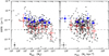Fig. 3.

Relation between the specific star formation rate and the stellar mass (left) and stellar mass surface density (right) for HI-normal (HI-def ≤ 0.4; filled dots) and HI-deficient (HI-def > 0.4; empty circles) galaxies. The large filled blue dots indicate the mean values for normal gas-rich systems, and the empty red dots show mean values for HI-deficient galaxies. The error bar shows the standard deviation of the distribution for the large symbols. The dashed line shows the limit between star-forming and quiescent galaxies. The typical uncertainty in the data is shown in the lower left corner of each panel.

4.2. Gas depletion timescale

Figure 4 shows the variation in HI gas depletion timescale as a function of stellar mass, stellar mass surface density, and specific star formation rate. Figure 4 shows a decrease in HI gas depletion timescale with increasing stellar mass and stellar mass surface density, while no evident trend is present as a function of specific star formation rate. Clearly, the HI gas reservoirs of dwarf galaxies and low surface brightness systems are able to sustain star formation at the current rate for more than 10 Gyr, while very massive objects (M_star ≥ 10¹⁰ M_⊙) can do this only for some billion years (see also McGaugh et al. 2017). The similarity in the HI gas depletion timescale measured in unperturbed gas-rich and perturbed gas-poor systems is striking, in particular, in the stellar mass range 10⁷ ≲ M_star ≲ 10⁹ M_⊙. We also note that the scatter in the τ_HI vs. M_star relation drawn by HI-rich systems (HI-def ≤ 0.4) increases with decreasing stellar mass.

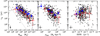Fig. 4.

Relation between the HI gas depletion timescale and stellar mass (left), stellar mass surface density (centre), and specific star formation rate (right) for HI-normal (HI-def ≤ 0.4; filled dots) and HI-deficient (HI-def > 0.4; empty circles) galaxies. The large filled blue dots indicate the mean values for each morphological class for normal gas-rich systems, and the empty red dots show mean values for HI-deficient galaxies. The error bar shows the standard deviation of the distribution for the large symbols. Upper limits are indicated by triangles and are treated as detections in the derivation of the mean values. The dotted line indicates the detection limit of the ALFALFA survey. The typical uncertainty in the data is shown in the lower left corner of each panel.

5. Main-sequence relation

5.1. General properties

Figure 5 shows the main-sequence relation derived with the 384 Hα detected galaxies analysed in this work. The improvement given by the unique set of data gathered in the VESTIGE survey is striking: it allows us to extend the main-sequence relation previously available for the Virgo cluster by ∼2 orders of magnitude. The relation now ranges between 10⁶ ≲ M_star ≲ 3 × 10¹¹ M_⊙ and 10⁻⁵ ≲ SFR ≲ 10 M_⊙ yr⁻¹. This dynamic range was never covered so far in any local or high-z sample.

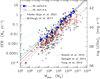Fig. 5.

Main-sequence relation for galaxies in the Virgo cluster coded according to their HI gas content: filled dots show HI gas-rich objects (HI-def ≤ 0.4), and empty circles represent HI-deficient objects (HI-def ≤ 0.4). Large solid blue and empty red circles are the mean values and standard deviations for HI-normal and HI-deficient objects. Star formation rates were derived assuming stationary conditions. The Y-axis on the right side gives the corresponding Hα luminosities corrected for dust attenuation. The solid black line is the best fit; obtained for gas-rich star-forming systems. The best fit is compared to those derived for bright galaxies with HI-def ≤ 0.4 included in the HRS (Boselli et al. 2015, bisector fit) and Speagle et al. (2014, derived extrapolating the time-dependent best-fit relation to z = 0), for the SDSS sample of Peng et al. (2010) derived for galaxies with M_star ≥ 10^8.5 M_⊙, for the local sample of Vilella-Rojo et al. (2021), and for the low surface brightness sample of McGaugh et al. (2017). The typical uncertainty on the data is shown in the lower left corner.

Following Boselli et al. (2015), we can consider galaxies with a normal HI gas content (HI-def ≤ 0.4; 56 objects) as unperturbed systems We derived the main-sequence relation by fitting the data using the linmix package for python⁴ (Kelly 2007), which considers in a Bayesian framework the uncertainties on both axes as well as an intrinsic scatter in the relation. The linear fit was made using a Markov chain Monte Carlo method to quantify the statistical uncertainties on the output parameters (see Fig. 5). The parameters derived from the fit are given in Table 2 using two different estimates of the uncertainties on the stellar mass and on the star formation rate. The first estimate considers only the uncertainties given by the SED fitting analysis (M_star) or derived through error propagation (SFR), and the second estimate adds an uncertainty related to the adopted models (see Sect. 3) in quadrature. To quantify any possible dependence of the fitted parameters on the adopted sample, we also derived the fitted relation using two different cuts in the HI-deficiency parameter (HI-def ≤ 0.3 and HI-def ≤ 0.5). Figure 6 shows the distribution of the orthogonal distance from the derived main-sequence relation for the whole sample and for the HI-normal galaxies (HI-def ≤ 0.4). Table 2 indicates that the slope of the fitted relation is robust to the adopted cut in the HI-deficiency parameter or the assumed uncertainties on the data. Figure 6 shows that galaxies with a normal HI gas content (HI-def ≤ 0.4) are symmetrically distributed on the derived best-fit relation.

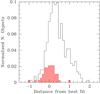Fig. 6.

Distribution of the orthogonal distance from the best fit of the main-sequence relation for the whole sample of galaxies (solid black histogram) and for the galaxies with a normal HI gas content (HI-def ≤ 0.4; hatched red histogram).

Table 2.

Coefficients of the main-sequence relation.

The slope (a = 0.92) is very close to the slope that was previously estimated for the HRS galaxies by Boselli et al. (2015) or for a large statistical sample of SDSS galaxies with M_star ≥ 10^8.5 M_⊙ by Peng et al. (2010). The slope, however, is significantly steeper than the one derived by Speagle et al. (2014), who extrapolated the time-dependent main-sequence relation to z = 0. This suggests that its determination in the local Universe is still highly uncertain. Its value is in between the value derived from the Javalambre-Photomteric Local Universe Survey (J-PLUS) local sample of Vilella-Rojo et al. (2021; a = 0.83) and the value of local low surface brightness galaxies of McGaugh et al. (2017; a = 1.04), which were both derived using Hα narrow-band imaging data. These two samples span a quite large dynamic range in stellar mass (10⁷ ≤ M_star ≤ 10¹¹ M_⊙), but are both dominated by objects with M_star ≥ 10⁸ M_⊙.

When limited to unperturbed systems (HI-def ≤ 0.4), the intrinsic scatter of the relation (σ ≃ 0.40) is comparable to that observed in other samples of local galaxies (e.g., Whitaker et al. 2012; Speagle et al. 2014; Ilbert et al. 2015; Gavazzi et al. 2015; Popesso et al. 2019; Vilella-Rojo et al. 2021). The relation does not show any evident bending at high masses (e.g., Bauer et al. 2013; Gavazzi et al. 2015; Popesso et al. 2019), although this effect might be hampered by the limited number of massive systems in this small sampled volume. It does not show any change of slope in the low stellar mass regime (M_star ≲ 10⁸ M_⊙) either, which is now sampled for the first time with an excellent statistics. There is, however, a significant increase in intrinsic scatter of the relation with decreasing stellar mass: σ ∼ 0.4 dex for the whole sample of HI-normal galaxies, σ ∼ 0.27 for massive systems (M_star > 10⁹ M_⊙), and σ ∼ 0.48 for dwarfs (M_star < 10⁹ M_⊙; see also Table 3). It is also interesting that the slope of the relation is very close for HI-normal (a = 0.92) and HI-deficient galaxies (a = 0.82), suggesting that the process that causes the gas depletion and the subsequent quenching of the star formation process acts in the same way at all stellar masses.

Table 3.

Average scaling relations.

5.2. Galaxies above the main sequence

Galaxies located above the main sequence are systems undergoing a starburst event that is often related to a merging episode (e.g., Rodighiero et al. 2011) or in clusters to a violent ram-pressure-stripping event (Vulcani et al. 2018). Ten objects (3% of the whole sample) with stellar mass M_star > 8 × 10⁶ M_⊙ are located at more than 1σ above the main-sequence relation (see Table 4). This fraction seems very limited when compared to the fraction observed in other samples of local cluster objects in Coma and A1367 (Boselli et al. 2022a; Pedrini et al. 2022) that undergo a ram-pressure-stripping event, or in the Gas Stripping Phenomena in Galaxies (GASP) sample of jellyfish galaxies (Vulcani et al. 2018; see Fig. 7). It is not possible to quantify the fraction of galaxies above the main sequence in these other samples, however, because they lack deep and complete untargeted surveys. VESTIGE is the only survey that includes a large number of star-forming systems of limited activity that are lacking in the other works, where most (if not all) of the observed galaxies were selected because of their strong star formation activity, peculiar morphology, and so on, and are thus not complete samples in any sense. These other selection criteria obviously favour objects with strong star formation activities as are expected for galaxies located above the main-sequence relation, which means that these samples are not suitable for driving statistical quantities. The low number of galaxies above the main sequence in the VESTIGE data with respect to the other samples, however, seems real given the limited number of catalogued late-type galaxies in these clusters, particularly in Coma, which is strongly dominated by the early types. This potential difference might have a physical reason. The Virgo cluster has a dynamical mass that is a factor of 10 lower than other massive clusters such as Coma and A1367. It is thus conceivable that the perturbing mechanisms at place in these more massive clusters are more efficient in perturbing their gas-rich members and triggering their star formation activity than in Virgo (e.g., Boselli et al. 2022a). There is, indeed, observational evidence that this is the case: (1) the spiral fraction in Virgo is significantly higher than in Coma (Boselli & Gavazzi 2006); (2) the fraction of HI-deficient galaxies, and the mean HI-deficiency of late-type galaxies, in Coma and A1367 is higher than in Virgo (Solanes et al. 2001; Boselli & Gavazzi 2006); (3) the increase of the radio continuum activity per unit far-infrared emission of galaxies in Coma and A1367 is higher than in Virgo (Gavazzi & Boselli 1999a,b; Boselli & Gavazzi 2006); and (4) the fraction of late-type galaxies with ionised gas tails, witnessing an ongoing ram-pressure-stripping process, is also higher in Coma and A1367 (∼50% Boselli & Gavazzi 2014; Yagi et al. 2010, 2017; Gavazzi et al. 2018b) than in Virgo, as revealed by the VESTIGE survey (Boselli et al., in prep.). Finally, (5) all these selection effects are expected to be even stronger in the GASP sample of jellyfish galaxies, where the selected objects (generally one or just a few per cluster) show the most extreme morphological perturbations.

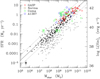Fig. 7.

Main-sequence relation for galaxies coded according to their distance to the best fit derived for HI gas-rich late-type systems. Filled black dots show galaxies within 1σ from the relation, and filled grey dots show galaxies > 1σ above or below the relation. The solid line gives the best fit obtained for gas-rich star-forming systems, and the dotted lines show the limits 1σ above and below the best fit. Galaxies undergoing a ram-pressure-stripping event identified in Boselli et al. (2022a) are indicated with large empty coloured symbols: brown circles show those belonging to the Norma cluster, green squares stand for Coma, and blue hexagons represent A1367. Red triangles indicate the jellyfish sample of Vulcani et al. (2018). Star formation rates and stellar masses are derived consistently with those measured within the Virgo cluster. The typical uncertainty on the data is shown in the lower left corner.

Observations (e.g., Gavazzi et al. 1995; Vollmer 2003; Vulcani et al. 2018) and simulations (Fujita & Nagashima 1999; Bekki 2014; Steinhauser et al. 2016; Steyrleithner et al. 2020; Troncoso-Iribarren et al. 2020; Boselli et al. 2021) consistently indicate that under some conditions, the star formation activity of cluster galaxies can be triggered by the compression of the gas during a ram-pressure-stripping process (Boselli et al. 2022a). The analysis of the morphological properties of the ionised gas in 15 Virgo cluster galaxies more than 1σ above the main sequence can help us to quantify how many of these objects are subject to this perturbing mechanism. We recall that the intrinsic scatter of the relation is σ = 0.40 dex, that is, the star formation activity of these objects increased by more than a factor of 2.5. The continuum-subtracted Hα images of all these objects are shown in Appendix B, and their physical parameters are given in Table 4. A large fraction of the sample is gas rich (four galaxies with HI-def ≤ 0.4 vs. six with HI-def > 0.4). This fraction includes two intermediate mass systems, VCC 801 (NGC 4383) and VCC 1554 (NGC 4532). Both show prominent filaments of ionised gas escaping from the galaxy disc, suggesting that an outflow of gas is triggered by the strong starburst activity. These morphological peculiarities are not typical of galaxies undergoing a ram-pressure-stripping event, where the ionised gas is rather compressed along a curved region at the leading edge of the interaction with the surrounding intra cluster medium (ICM) and a low surface brightness tail forms at the opposite side (typical examples are CGCG 97-73 in A1367, Gavazzi et al. 1995, 2001; and IC 3476 in Virgo; Boselli et al. 2021). They are rather typical in merging systems such as M 82 (Shopbell & Bland-Hawthorn 1998; Mutchler et al. 2007). The remaining galaxies, all dwarfs with 8×10⁶ < M_star < 2 × 10⁹ M_⊙, are mainly BCDs (six out of ten) or irregulars in which the star formation activity is often concentrated in a few bright and giant HII regions. Their burst activity is evident, but not always related to an external perturbing mechanism. We can thus conclude that in a cluster such as Virgo (a few 10¹⁴ M_⊙), ram-pressure stripping, identified as the dominant perturbing mechanism (e.g., Boselli et al. 2014c, 2022a), does not significantly increase the star formation activity of the perturbed galaxies on average. If this happens, it occurs on very short timescales (Boselli et al. 2021), so that the probability of observing galaxies with an increased activity remains very low.

Table 4.

Galaxies at more than 1σ above the main sequence.

5.3. Origin of the scatter

When measured on the whole sample, the observed relation has a strong scatter (∼1 dex) at all stellar masses, significantly stronger than the scatter that is observed in other samples of local galaxies (≲0.3 dex). This large scatter is mainly due to objects that are located below the main-sequence relation drawn by representative samples of field galaxies or by unperturbed objects within the Virgo cluster (HI-def ≤ 0.4). The limited number of objects in the starburst sequence that formed by merging systems observed in other Hα selected samples at high redshift (Caputi et al. 2017) and rare in the local Universe (Rodighiero et al. 2011; Sargent et al. 2012) are lacking here. As already noted by Boselli et al. (2015), the scatter in the relation is strongly related to the HI-deficiency parameter, suggesting that the reduced activity of star formation typical of these quenched cluster galaxies is tightly connected to their atomic gas reservoir (see Fig. 8). This is clear in Fig. 9, where the offset from the main-sequence relation drawn by unperturbed HI-rich systems (HI-def ≤ 0.4) is plotted against the HI-deficiency parameter. Figure 9 indeed shows a tight relation between the offset of galaxies from the main-sequence relation and the amount of HI gas that is available in them.

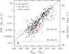Fig. 8.

Main-sequence relation for galaxies coded according to their morphological type and HI gas content: Late-type galaxies (≥Sa) are indicated by black symbols, and early-type galaxies are shown by red symbols. Filled dots are for HI gas-rich objects (HI-def ≤ 0.4), and HI-deficient objects (HI-def > 0.4) are shown by empty circles. Star formation rates were derived assuming stationary conditions. The Y-axis on the right side gives the corresponding Hα luminosities corrected for dust attenuation. The solid line is the best fit obtained for gas-rich star-forming systems. The horizontal dotted and dashed lines indicate the corresponding SFR derived using the number of ionising photons produced by an O3 class III and a B0 class III star as derived using the model atmospheres of Sternberg et al. (2003). The typical uncertainty on the data is shown in the lower left corner.

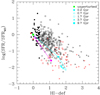Fig. 9.

Relation between the offset from the main-sequence relation log SFR/SFR_MS and the HI-deficiency parameter: Late-type galaxies (≥Sa) are indicated by black symbols, early-type galaxies by red symbols, circles stand for HI detected sources, and triangles stand for HI undetected objects (lower limits to the HI-deficiency parameter). Filled symbols show HI gas-rich objects (HI-def ≤ 0.4), and empty symbols show HI-deficient objects (HI-def > 0.4). The data are compared to the predictions of models for starvation (magenta) and ram-pressure stripping (cyan) derived for a galaxy with a rotational velocity 70 km s⁻¹ and spin parameter λ = 0.05. The filled green square indicates the prediction for an unperturbed system. Different symbols in the models indicate the position of the model galaxies at a given look-back time from the beginning of the interaction.

The tight connection of the star formation activity with the total atomic gas content, which are both reduced in cluster galaxies, has previously been noted (e.g., Gavazzi et al. 2002, 2013; Boselli et al. 2014c). Although the atomic gas does not directly participate in the star formation process, which rather depends on the molecular gas phase (e.g., Bigiel et al. 2008), it is the principal supplier of the giant molecular clouds in which star formation takes place. Since a large fraction of the HI gas is located in the outer galaxy regions, infall of atomic gas into the stellar disc has been invoked to explain the observed strong correlation between the total gas content and star formation in local galaxies (e.g., Boselli et al. 2001). The tight connection between the star formation activity and the atomic gas content also suggests that the conversion rate from atomic to molecular gas is roughly proportional to the atomic gas mass. This is deduced by the fact that (a) the star formation rate is tightly related at large scales to the total molecular gas content (e.g., Kennicutt 1998b; Boselli et al. 2002) and at smaller scales (∼500 pc) to the molecular gas column density (e.g., Bigiel et al. 2008), and (b) the atomic gas consumption time is similar for galaxies, regardless of their HI deficiency (in a limited but broad mass range; see Sect. 4.2). We recall that an accurate estimate of the gas consumption timescale would require determining the molecular gas content, which is unfortunately unknown in this sample that is dominated by low-mass and low-metallicity systems, in which the detection of the CO line emission is challenging. There is some evidence that the molecular gas phase is also reduced in HI-deficient objects, although at a lower level than the atomic gas (e.g., Fumagalli et al. 2009; Boselli et al. 2014b; Mok et al. 2017).

The observed scatter in the relation exceeds the scatter previously observed for Virgo galaxies in the high stellar mass range (10⁹ ≲ M_star ≲ 10¹¹ M_⊙). The VESTIGE sample includes objects with an even more reduced star formation activity than in the HI-deficient Virgo galaxies belonging to the HRS. Figure 8 indicates that these most extreme objects are mainly early-type galaxies with low Hα emission. In most of these objects, the Hα emission is clearly related to an ongoing star formation activity in the inner regions, which are mainly located in rotating discs, and in only a few cases is the ionised gas emission associated with filaments in which the ionising radiation could be also produced by cooling flows or shocks (M 87, NGC 4262, NGC 4552; Gavazzi et al. 2000, 2018a; Boselli et al. 2019, 2022b). In the low stellar mass range (M_star ≲ 10⁹ M_⊙), these early-type galaxies are dwarf systems with a residual star formation activity in their nucleus, as first noted by Boselli et al. (2008a). These early types with a residual star formation activity were mainly lacking in previous Hα surveys, such as the follow-up observations of the HRS (Boselli et al. 2015), which targeted only late-type systems, but which are present and frequent in blind surveys such as VESTIGE.

5.4. Comparison with models of ram-pressure stripping and starvation

Several perturbing mechanisms have been proposed in the literature to explain the reduced activity of star formation in cluster galaxies (e.g., Boselli & Gavazzi 2006, 2014). Among these, the mechanism that is generally invoked to explain the observed properties of nearby cluster galaxies, such as cometary tails of gas in its different phases without any associated stellar structure, or truncated gaseous discs versus unperturbed stellar discs, is ram-pressure stripping (Gunn & Gott 1972; see the recent review of Boselli et al. 2022a for details). This stripping process also appears to be dominant within the Virgo cluster, as indicated by several statistical studies (e.g., Vollmer et al. 2001b; Vollmer 2009; Boselli et al. 2008a,b, 2014c,b; Gavazzi et al. 2013) or observations of representative objects (Vollmer et al. 1999, 2000, 2001a, 2004a,b, 2006, 2008a,b, 2012, 2018, 2021; Vollmer 2003; Yoshida et al. 2002, 2004; Kenney et al. 2004, 2014; Crowl et al. 2005; Boselli et al. 2006, 2016a, 2021; Chung et al. 2007; Pappalardo et al. 2010; Abramson et al. 2011, 2016; Abramson & Kenney 2014; Sorgho et al. 2017; Fossati et al. 2018; Cramer et al. 2020).

The observed scatter in the main-sequence relation is also consistent with this picture, as is indicated by the prediction of tuned ram-pressure-stripping models (see Fig. 10). These physically motivated models, which were first introduced by Boselli et al. (2006) to explain the truncated gas and star-forming disc of NGC 4569, have been successfully used to predict the evolution of the chemo-spectrophotometric 2D properties of dwarf systems (Boselli et al. 2008a,b), diffuse galaxies (Junais et al. 2021, 2022), and the normal quenched galaxy population of the Virgo cluster (Boselli et al. 2014c, 2016b). These models, which are extensively described in the references, are based on the multizone chemo-spectrophotometric models of galaxy evolution of Boissier & Prantzos (2000) that were updated with an empirically determined star formation law (Boissier et al. 2003) relating the star formation rate to the total gas surface density. This last is modulated by the rotational velocity of the galaxy,

$\begin{matrix} Σ_{SFR} = α Σ_{gas}^{1.48} V (R) / R, \end{matrix}$ $\begin{aligned} {\Sigma _{\rm SFR} = \alpha \Sigma _{\rm gas}^{1.48}V(R)/R} ,\end{aligned}$ (12)

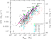Fig. 10.

Comparison of the observed main-sequence relation with the predictions of ram-pressure-stripping models for galaxies with a spin parameter λ = 0.05 and rotational velocities of 40, 70, 130, and 220 km s⁻¹. Unperturbed models are indicated with filled green squares, starvation models by the magenta lines, and ram-pressure-stripping models by the cyan lines. Different symbols for the models indicate the position of the model galaxies at a given look-back time from the beginning of the interaction. Black (red) filled circles show late-type (early-type) galaxies with a normal HI content (HI-def ≤ 0.4), and black (red) empty circles show HI-deficient (HI-def > 0.4) late-type (early-type) systems. The typical uncertainty on the data is shown in the lower left corner.

where V(R) is the rotational velocity at radius R. Galaxies are treated as exponential discs embedded in a spherical dark matter halo, characterised by two free parameters: the rotational velocity of the system, which is tightly connected with its total dynamical mass, and the spin parameter λ, which rather traces the distribution of the angular momentum. The models also include a radially dependent infall rate of pristine gas that decreases exponentially with time. The parameters regulating the infall rate were calibrated to reproduce the colour and metallicity gradients of isolated galaxies (Prantzos & Boissier 2000; Muñoz-Mateos et al. 2011).

To reproduce the perturbations induced by the surrounding environment, we simulated a ram-pressure-stripping process as in Boselli et al. (2006). The ram-pressure-stripping event was simulated by assuming a gas-loss rate inversely proportional to the gravitational potential of the galaxy ϵΣ_gas/Σ_potential, with an efficiency ϵ depending on the IGM gas density radial profile of the Virgo cluster, here taken from Vollmer et al. (2001b).

To limit the number of free parameters, we considered only models with a fixed spin parameter of λ = 0.05, the typical value of normal late-type galaxies predicted by cosmological simulations (Mo et al. 1998) and derived from observations of unperturbed field objects (Muñoz-Mateos et al. 2011), while we varied the rotational velocity of galaxies from 20 to 300 km s⁻¹ to consider a wide range of dynamical masses. Adopting a wider range of spin parameters more representative of a complete galaxy distribution would slightly increase the scatter of the main-sequence relation for unperturbed systems. For the ram-pressure-stripping model, we assumed the same stripping efficiency as derived for NGC 4569 (ϵ₀ = 1.2 M_⊙ kpc⁻² yr⁻¹) that was proved to reproduce the 2D properties of large samples of Virgo cluster objects well.

Since the gravitational potential well of the galaxies decreases with galactocentric distance, the models predict that the gas is stripped outside-in, producing truncated gas discs such as those typically observed in the HI maps of Virgo galaxies (e.g., Warmels 1986; Cayatte et al. 1990, 1994; Chung et al. 2009) or in the other components of the ISM (molecular gas, Fumagalli et al. 2009; Boselli et al. 2014b; Mok et al. 2017; dust, Cortese et al. 2010, 2014; Longobardi et al. 2020; Boselli et al. 2022a). The lack of gas reduces the activity of star formation, producing similar truncated discs in the youngest stellar populations (e.g., Koopmann & Kenney 2004b,a; Koopmann et al. 2006; Fossati et al. 2013; Boselli et al. 2015). The perturbed galaxies become redder in colour because of the ageing of the stellar populations, which is not supplied by the formation of new stars on the discs (Boselli et al. 2014c). We recall that these models assume a face-on stripping process. This is a very simplified approach because the inclination of galaxies changes along their parabolic orbit through the ICM. Because the efficiency of stripping is known to vary as a function of the inclination (e.g., Roediger & Brüggen 2006), this makes the reconstruction of the star formation history of the perturbed galaxies quite uncertain.

For comparison, we also include a starvation scenario (e.g., Larson et al. 1980; Balogh et al. 2000; Treu et al. 2003), modelled by stopping the infall of pristine gas necessary to reproduce the observed colour and metallicity gradients of star-forming discs. The starved galaxy then becomes anemic simply because it exhausts its gas reservoir through ongoing star formation. As defined, starvation is a passive phenomenon, where the gas is exhausted via star formation. For this reason, the simulated starvation process is much less efficient than ram pressure in quenching the activity of star formation of the perturbed galaxies (Boselli et al. 2006, 2014c).

The prediction of the models are compared to observations in Fig. 10. Unperturbed model galaxies follow the main-sequence relation, albeit with a slightly higher star formation activity than is observed in Virgo late-type systems with a normal HI gas content. When the cluster is crossed, however, ram pressure can remove a sufficient amount of atomic gas to significantly reduce their activity of star formation. At 0.7 Gyr after the beginning of the interaction, the star formation rate can be reduced by an order of magnitude in massive systems (M_star ≥ 10¹⁰ M_⊙), which increases to up to more than two orders of magnitude in the low-mass regime (M_star ≲ 10⁹ M_⊙). The models indicate that this quenching episode occurs on relatively short timescales (≲700 Myr) compared to the typical crossing time of the cluster (≃1.7 Gyr), in line with previous observations of statistical samples (e.g., Crowl & Kenney 2008; Boselli et al. 2008a, 2016b; Ciesla et al. 2021) or of representative Virgo cluster objects (Vollmer et al. 1999, 2004a,b, 2006, 2008a,b, 2012, 2018, 2021; Boselli et al. 2006; Fossati et al. 2018). In contrast, starvation, which is a mild process, is not able to significantly reduce the activity of star formation of the perturbed galaxies such as the one observed in the VESTIGE sample, and this holds for galaxies of all stellar masses. In this scenario, the star formation activity can be reduced by a factor of 2–3 at most, but this requires very long timescales, of the order of several billion years (Boselli et al. 2006, 2014c).

Since high-sensitivity multifrequency observations, models, and simulations of selected targets unambiguously identified several objects undergoing a ram-pressure-stripping event in the Virgo cluster (see Table 2 in Boselli et al. 2022a for details), we can see how these objects are located within the main-sequence relation (see Fig. 11). Figure 11 confirms that the scatter of the relation is dominated by galaxies with a lower-than-expected star formation activity. Among those identified as subject to a ram-pressure-stripping event (24 objects), 17 are located within 1σ from the main sequence, none is located above the main sequence, and 7 are located below it. Although this subsample of objects is not statistically complete, it confirms that overall the activity of star formation of ram-pressure-stripped galaxies, if perturbed, is reduced. Figure 11 also shows, however, that in a few objects, the star formation activity might be higher than that of typical main-sequence galaxies. This occurs mainly at low stellar masses and might be due to (i) an increased activity because the gas in the disc of the galaxy is compressed at a particular and specific phase of the stripping process (e.g., Boselli et al. 2021, 2022a), or (ii) an inaccurate determination of the star formation rate in these low-mass regimes for the several reasons mentioned in Sect. 3.4. The detailed analysis of these galaxies presented in see Sect. 5.2 and in Appendix B suggests that their higher activity is often but not always due to a ram-pressure-stripping event. Finally, we stress that the fact that several star-forming galaxies are located below the main-sequence relation, or equivalently, in the green valley located between the red sequence and the blue cloud (e.g., Boselli et al. 2014c), is not a direct indication that the quenching mechanism acts on long timescales (e.g., Paccagnella et al. 2016) just because it does not take the high infall rate of galaxies within the cluster into account, which for Virgo is estimated at ∼200–300 objects Gyr⁻¹ for galaxies of M_star ≥ 10⁹ M_⊙ (Boselli et al. 2008a; Gavazzi et al. 2013; Sorce et al. 2021).

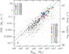Fig. 11.

Main-sequence relation for galaxies coded according to their distance from the best fit derived for HI gas-rich late-type systems. Filled black dots show galaxies within 1σ from the relation, and filled grey dots show galaxies > 1σ above or below the relation. The solid line is the best fit obtained for gas-rich star-forming systems, and the dotted lines show the limits 1σ above and below the best fit. Galaxies undergoing a ram-pressure-stripping event identified in Boselli et al. (2022a) are indicated with coloured squares, and those subjected to a combined effect of ram pressure and harassment are shown by triangles. The typical uncertainty on the data is shown in the lower left corner.

5.5. Evolutionary state of the perturbed galaxies

The evolutionary path of galaxies within a cluster environment is very complex and depends on several parameters, such as the properties of the high-density region (ICM distribution, density, and temperature), of the impact parameters of galaxies along their orbits within the cluster (radial, circular, and infalling as isolated objects or as members of small groups), on the properties of galaxies (total mass, gas content, and distribution), and on the epoch in which the infall occurs. Furthermore, different mechanisms can contribute at different epochs to modify the galaxy evolution. The reconstruction of the orbit of a single galaxy within a cluster, the measurement of the main impact parameters, the identification of the dominant stripping process, and the reconstruction of the following evolution of the different stellar populations require accurate models and simulations that are specifically tuned to reproduce the observed 2D spectrophotometric and kinematical properties of the perturbed objects. As mentioned in Sect. 5.3, this has only been done for a few objects in Virgo. A general evolutionary picture, however, can be driven by comparing the statistical properties of a complete sample of galaxies such as the one analysed in this work with the prediction of cosmological simulations. This is generally done by means of the phase-space diagram, which shows the position of the selected galaxies defined as the relative velocity versus the mean velocity of the cluster normalised to the velocity dispersion of the cluster itself as a function of the clustercentric distance (e.g., Mahajan et al. 2011; Haines et al. 2015; Jaffé et al. 2015, 2018; Rhee et al. 2020). This exercise has been performed for galaxies within the Virgo cluster (e.g., Vollmer et al. 2001b,a; Boselli et al. 2014c; Yoon et al. 2017; Morokuma-Matsui et al. 2021).

Figure 12 shows the distribution of the Hα detected galaxies within the phase–space diagram of the Virgo cluster, with galaxies coded according to their atomic gas content and morphological type as in Fig. 8. The distribution of galaxies within this diagram is compared to that predicted by the cosmological simulations of Rhee et al. (2017), which give a general trend as a function of the epoch of first infall. We recall that these simulations give just a statistically weighted trend, and can thus be considered in the comparison only in these terms. Figure 12 does not show any statistically significant trend in the distribution of the HI-rich and HI-deficient galaxies within the phase-space diagram.

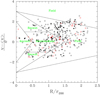Fig. 12.

Phase-space diagram for the Hα detected galaxies within the Virgo cluster. For all galaxies, the X-axis indicates the projected distance from the central galaxy M87 in units of r₂₀₀, and the Y-axis shows the excess in velocity with respect to the mean velocity of cluster A (⟨v⟩ = 955 km s⁻¹) normalised to its mean velocity dispersion (σ = 799 km s⁻¹; Boselli et al. 2014c). Late-type galaxies (> Sa) are indicated by black symbols, and early-type galaxies are shown by red symbols. Filled dots show HI gas-rich objects (HI-def ≤ 0.4), and HI-deficient objects (HI-def > 0.4) are shown by empty circles. The solid lines delimit the different regions extracted from the simulations of Rhee et al. (2017) to identify galaxies in different phases of their infall into the cluster: first (not yet fallen), recent (0 < τ_inf < 3.6 Gyr), intermediate (3.6 < τ_inf < 6.5 Gyr), and ancient (6.5 < τ_inf < 13.7 Gyr) infallers.

We repeated the exercise by dividing galaxies according to their position along the main sequence. For this purpose, we divided the main-sequence relation into four main subsamples, as indicated in Fig. 13: normal galaxies, located within 1σ from the best fit derived for the subsample of HI-normal galaxies (HI-def ≤ 0.4), where σ is the dispersion of the relation (0.40 dex); starburst galaxies, located at more than 1σ above the relation, partly quenched galaxies (1σ < s ≤ 3σ), and quenched systems (s > 3σ), where s is the distance perpendicular to the main-sequence relation.

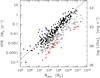Fig. 13.

Main-sequence relation for galaxies coded according to their distance from the best fit derived for HI gas-rich late-type systems. Filled black dots show galaxies within 1 σ from the relation, filled blue dots show galaxies > 1σ above the relation, empty black circles show galaxies 1σ–3σ below the relation, and filled red dots show galaxies > 5σ below the relation. The solid line is the best fit obtained for gas-rich star-forming systems. The typical uncertainty on the data is shown in the lower left corner.

Figure 14 shows the distribution of galaxies within the phase–space diagram with galaxies coded according their distance from the main sequence, as indicated in Fig. 13. Figure 14 does not show any evident trend in the distribution of the different class of star-forming objects. Since ram-pressure stripping, identified in Virgo as the dominant gas-stripping mechanism, strongly depends on the total mass of the perturbed galaxies (in massive systems, the deep gravitational potential well can more efficiently keep the cold gas anchored to the stellar disc than in dwarf systems, where the gas is easily and completely stripped on short timescales), we plot in Figs. 15 and 16 the distribution of the selected galaxies in the phase-space diagram coded according to their atomic gas content and star formation activity in three bins of stellar mass: M_star > 10^9.5 M_⊙, massive systems; 10⁸ < M_star ≤ 10^9.5 M_⊙, intermediate mass systems; and M_star ≤ 10⁸ M_⊙, dwarfs.

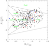Fig. 14.

Phase–space diagram for galaxies coded according to their distance from the best fit derived for HI gas-rich late-type systems. Filled black dots show galaxies within 1σ from the relation, filled blue dots show galaxies > 1σ above the relation, empty circles show galaxies 1σ–3σ below the relation, and filled dots show galaxies > 5σ below the relation. The solid lines delimit the different regions extracted from the simulations of Rhee et al. (2017) to identify galaxies in different phases of their infall into the cluster: first (not yet fallen), recent (0 < τ_inf < 3.6 Gyr), intermediate (3.6 < τ_inf < 6.5 Gyr), and ancient (6.5 < τ_inf < 13.7 Gyr) infallers.

As for the previous plots, Figs. 15 and 16 do not show any strong systematic segregation in the distribution of the HI-deficient and HI-rich galaxies or star-forming and quenched objects within the phase-space diagram. However, Virgo is a cluster still in formation, as suggested by the several subgroups. Its 3D structure is thus very complex and hardly schematised in spherical geometry. Under this configuration, any systematic effect in the galaxy distribution within this diagram can be heavily smeared out by projection effects. However, HI-rich galaxies are already rare in the infalling regions (15% of the star-forming systems, with respect to ∼70% in the field; Cattorini et al. 2022). This means that the dominant perturbing mechanism is (1) already active at the periphery of the cluster (R/r₂₀₀ ≥ 1), and (2) efficiently removes the atomic gas content on short timescales (≲1 Gyr), otherwise galaxies would have retained their gas reservoir along their orbits up to the inner regions. The similar distribution of star-forming galaxies within the phase-space diagarm consistently indicates that, as for the gas removal, the star formation process is also quenched on short timescales, as expected in a ram-pressure-stripping scenario (e.g., Boselli et al. 2008a, 2014c, 2016b).

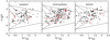Fig. 15.

Phase–space diagram in three different bins of stellar mass (M_star > 10^9.5 M_⊙, massive; 10⁸ < M_star ≤ 10^9.5 M_⊙, intermediate; and M_star ≤ 10⁸ M_⊙, dwarfs) for galaxies coded according to their morphological type (black symbols for late types, and red symbols for early types) and atomic gas content (filled dots for HI gas-rich objects (HI-def ≤ 0.4), and empty circles show HI-deficient objects (HI-def > 0.4)). The solid lines delimit the different regions extracted from the simulations of Rhee et al. (2017) to identify galaxies in different phases of their infall into the cluster: first (not yet fallen), recent (0 < τ_inf < 3.6 Gyr), intermediate (3.6 < τ_inf < 6.5 Gyr), and ancient (6.5 < τ_inf < 13.7 Gyr) infallers.

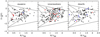Fig. 16.

Phase–space diagram in three different bins of stellar mass (M_star > 10^9.5 M_⊙, massive; 10⁸ < M_star ≤ 10^9.5 M_⊙, intermediate; and M_star ≤ 10⁸ M_⊙, dwarfs) for galaxies coded according to their distance from the main-sequence relation derived for gas-rich late-type systems: filled black dots show galaxies within 1σ from the relation, filled blue dots show galaxies > 1σ above the relation, empty black circles show galaxies 1σ–3σ below the relation, and filled red dots show galaxies > 3σ below the relation. The solid lines delimit the different regions extracted from the simulations of Rhee et al. (2017) to identify galaxies in different phases of their infall into the cluster: first (not yet fallen), recent (0 < τ_inf < 3.6 Gyr), intermediate (3.6 < τ_inf < 6.5 Gyr), and ancient (6.5 < τ_inf < 13.7 Gyr) infallers.

5.6. Extension to lower stellar mass

The VESTIGE survey has also detected several HII regions located well outside the star-forming discs of Virgo cluster galaxies formed within the gas stripped during the interaction with the surrounding environment. Typical examples of these extraplanar star-forming regions are those detected in the tail of IC 3418 that probably formed after a ram-pressure-stripping event (VCC1217; Hester et al. 2010; Fumagalli et al. 2011a; Hota et al. 2021), those located in between UGC 7636 and M49 that formed by a combined effect of ram-pressure stripping within the halo of M 49 and gravitational interactions between the two galaxies (VCC 1249; Arrigoni Battaia et al. 2012), or those located along the long HI tail of NGC 4254 that formed after a gravitational perturbation in a high-speed fly-by encounter with another cluster member (Vollmer et al. 2005; Duc & Bournaud 2008; Boselli et al. 2018b). It has been claimed that these regions, characterised by stellar masses of 10³ ≲ M_star ≲ 10⁵ M_⊙ and star formation rates of 10⁻⁵ ≲ SFR ≲ 10⁻³ M_⊙ yr⁻¹, might become gravitationally unbound systems and thus be at the origin of compact objects such as globular clusters or ultra-compact dwarf galaxies (UCDs) typical of rich environments. As stressed in Boselli et al. (2018b), UCDs have stellar masses higher than those observed in these star-forming regions (Liu et al. 2020). They might have been formed in the past, when galaxies were much more gas rich than in the local Universe, by a similar perturbing mechanism that was able to remove larger quantities of gas. When we consider these objects as unbound systems representative of the compact galaxy population, we can see how they populate the main-sequence relation in comparison to more extended systems. This exercise can be made for the extraplanar regions of NGC 4254, where star formation rates and stellar masses are available for ≃60 objects (Boselli et al. 2018b; see Fig. 17). These extraplanar HII regions were identified in the FUV GALEX band. Their stellar masses and star formation rates were derived using CIGALE on their observed FUV-to-z SEDs, as was done for the VESTIGE galaxies, but adopting a realistic delayed exponentially declining star formation history with parameters representative of individual HII regions (see Boselli et al. 2018b for details). Stellar masses and star formation rates given in Boselli et al. (2018b) were divided by 1.64 and 1.58, respectively, to convert the original estimates based on a Salpeter IMF into a Chabrier IMF. To avoid any possible systematic bias in the comparison, this plot was made using either the star formation rates derived from the SED fitting modelling or the rates that were directly measured from the VESTIGE Hα fluxes corrected for [NII] contamination and dust attenuation, as for the rest of the sample galaxies.

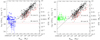Fig. 17.

Main-sequence relation including extraplanar HII regions. Left panel: relation between the Hα luminosity (corrected for dust attenuation) and stellar mass for galaxies coded according to their morphological type and HI gas content: late-type galaxies (> Sa) are indicated by black symbols, and early-type galaxies by red symbols. Filled dots show HI gas-rich objects (HI-def ≤ 0.4), and HI-deficient objects (HI-def > 0.4) are shown by empty circles. The solid line is the best fit obtained for gas-rich star-forming systems. Blue triangles show the extraplanar HII regions detected in NGC 4254 (Boselli et al. 2018b), where stellar masses and star formation rates have been determined using the SED fitting code CIGALE. Filled triangles show Hα detected regions, and empty triangles stand for the undetected ones. The error bars of the HII regions of NGC 4254 are those given by the SED fitting analysis. The horizontal dotted and dashed lines indicate the corresponding SFR derived using the number of ionising photons produced by an O3 class III and a B0 class III star as derived using the model atmospheres of Sternberg et al. (2003). The dot-dashed red line indicates the corresponding completeness limit of VESTIGE at the mean distance of Virgo (16.5 Mpc). The right Y-axis gives the corresponding SFR (main-sequence relation) derived assuming stationary conditions. Right panel: similar plot, in which the green filled triangles are the extraplanar HII regions of NGC 4254 detected in Hα, where the stellar masses are derived using the SED fitting analysis with CIGALE, while the star formation rates are measured using the same calibration based on the Hα luminosity as for the galaxy sample, assuming A(Hα) = 0.7 mag and [NII]λ6584 Å/Hα = 0.2, as in Boselli et al. (2018b). The uncertainties on the stellar mass of the HII regions of NGC 4254 are given by the fitting code CIGALE, and those on their star formation rate indicate the dynamic range in this parameter assuming either A(Hα) = 0 mag or A(Hα) = 1.5 mag.

Figure 17 clearly shows that these extraplanar star-forming regions do not follow the main-sequence relation drawn by the rest of the Virgo cluster galaxies. They are characterised by much higher star formation rates than are expected for their low stellar mass, which should be approximately 10⁻⁸ ≲ SFR ≲ 10⁻⁵ M_⊙ yr⁻¹. We recall, however, that these star formation rates are too low to produce a statistically significant number of ionising stars because of a poor sampling of the IMF in the high-mass stellar regime. As a consequence, they cannot be measured using a Hα survey. This is indeed confirmed by the lack of any Hα emitting source with a luminosity L(Hα)≲10^36.5 erg s⁻¹, the typical Hα luminosity of an early-B star (the regions for which the star formation rates were derived with the SED fitting analysis of SFR ≲ 2 × 10⁻⁵ M_⊙ yr⁻¹ are shown in the left panel of Fig. 17; they are not detected in Hα). Despite this strong selection effect, which can justify the lack of Hα emitting sources at low star formation rates (SFR ≲ 2 × 10⁻⁵ M_⊙ yr⁻¹), the star formation rates of these extraplanar HII regions are two to three orders of magnitudes higher per unit stellar mass than those of normal star-forming galaxies that populate the main sequence. This spectacular difference can be explained when we consider these HII regions as short-lived starbursts, as is suggested by their star formation history derived in the SED fitting analysis (Boselli et al. 2018b). Their activity lasts only for a few million years (≲50 Myr) and gradually stops to form quenched systems. They are thus unstable objects, and their presence above the main sequence is a temporary effect lasting only for short times. As extensively discussed in Boselli et al. (2018b), many of these regions have already completed their starburst phase and are becoming increasingly redder. They witness an ageing stellar population.

6. Discussion

6.1. Completeness

The exceptional depth of the VESTIGE survey allows us to trace the main-sequence relation and other important scaling relations for a nearby rich cluster of galaxies down to stellar masses of a few 10⁶ M_⊙ and star formation rates of a few 10⁻⁵ M_⊙ yr⁻¹, sampling thus a dynamic range that was never reached before in any other sample of isolated or cluster galaxies. In particular, the sensitivity of the narrow-band imaging data (f(Hα)≃4 × 10⁻¹⁷ erg s⁻¹ cm⁻² (5σ) for point sources) corresponds to a limit in the Hα luminosity of L(Hα)≃10³⁶ erg s⁻¹ at the distance of Virgo, a value slightly lower than the expected luminosity due to the ionising photons produced by a single early-B star. This means that the VESTIGE survey samples the whole range of Hα luminosity of galaxies down to the lowest possible star formation rates that are physically measurable with Hα data. Since at these low luminosities, the emission associated with dwarf galaxies is generally attributable to a very few ionising stars (≲3), it is possible that the measured fluxes are contaminated by background line emitters. Following Sun et al. (2007), we can estimate that the number of Lyα line emitters at z ∼ 4.1 that can be detected within one square degree is about 200 at the sensitivity of VESTIGE. When we consider that at the distance of the cluster, the typical size of dwarf galaxies of M_star ≃ 10⁶ − 10⁷ M_⊙ is ∼1′ in diameter, the probability that a background line emitter falls within the projected image of a dwarf galaxy is ≃4%. The contamination of background galaxies is thus certainly negligible. Conversely, we might lose some Virgo cluster objects if their Hα emission is limited to a point source without any extended emission and the galaxy has such a peculiar morphology that it cannot be identified as a cluster member using the typical scaling relations derived in the NGVS (Lim et al. 2020). Since we detected only five emitting sources over the 384 identified by VESTIGE with an extended Hα morphology suggesting their cluster membership that were not included in the NGVS catalogue of 3689 Virgo members, we expect that the number of Hα emitting sources associated with the cluster that were missed by VESTIGE is very limited.

6.2. Accuracy of the SFR determination

The narrow-band imaging data used in this work were corrected for [NII] contamination and dust attenuation before they were transformed into star formation rates. These corrections are important sources of uncertainties in the determination of an accurate star formation rate of massive galaxies, where dust attenuation and [NII] contamination are relevant. For all the massive galaxies, we estimated the [NII] contamination using long-slit integrated spectroscopy, and we applied two different dust attenuation corrections based on integrated spectroscopy and far-IR emission. As extensively discussed in Boselli et al. (2015), the combination of these independent techniques are optimal for minimising the uncertainties and provide the most accurate results (see also Calzetti et al. 2007, 2010; Kennicutt et al. 2009). The same set of data, however, was only sporadically available for dwarf systems, for which we applied (if any) corrections based on scaling relations. In this metal- poor galaxy population, however, both [NII] contamination and dust attenuation, if present, are very low (e.g., Boselli et al. 2009), thus their possible impact on the determination of the star formation rate of galaxies is negligible.

A more important source of uncertainty in this regime of low star formation rate might be the non-stationary conditions and the stochastic sampling of the IMF. Stationary conditions are reached whenever the number of massive stars that cause the Hα emission of a galaxy formed per unit time equals that of the same stars leaving the main sequence, that is, that the star formation rate of the galaxy is constant on timescales longer than the typical age of the ionising stellar population (≲10 Myr).

This stationary condition is certainly not satisfied in dwarf systems, in which the total Hα emission is due to a very limited number of ionising stars and/or star clusters that might turn on or off in a stochastic way during the star formation history of the galaxy (e.g., Boselli et al. 2009). At these very low star formation rates, the gaps occurring in between episodes of formation of individual clusters can lead to irregular and highly bursty star formation histories, as suggested by models that rely on sampling of the cluster mass function (Fumagalli et al. 2011b; da Silva et al. 2012), numerical simulations (Flores Velázquez et al. 2021), and observations (Emami et al. 2019). Although somewhat sub-dominant compared to the burstiness, the stochastic sampling of the IMF could lead to further scatter in the luminosity of low-mass galaxies. This effect is instead highly relevant for individual HII regions (Elmegreen 2000; Cerviño et al. 2003, 2013; Cerviño & Luridiana 2004; Koda et al. 2012). The intrinsic burstiness and the sampling of the IMF are expected to not only introduce scatter in the correlations presented in this work, but also to induce a bias in the estimates of the SFR for most of the range we examined (see e.g., da Silva et al. 2014). We also note that due to the presence of HI deficient galaxies that down-scatter from the main sequence, the effects of burstiness and stochasticity are not readily noticeable as an increased scatter in the main sequence measured on the whole sample. They might, however, cause the observed increase in the scatter at low stellar masses in the HI gas-rich population (see Table 3). We recall that the intrinsic scatter of the relation is ∼0.40 dex for the full sample of galaxies with HI-def ≤ 0.4, ∼0.27 dex when limited to massive objects (M_star > 10⁹ M_⊙) and ∼0.48 in dwarf systems (M_star ≤ 10⁹ M_⊙). We can also add that whenever the few emitting sources are located far away from each other on an extended stellar disc, the adopted flux extraction procedure, which uses a large aperture, gives large uncertainties because of a possible variation of the background within the aperture. Overall, these effects might increase the scatter of the main-sequence relation at low luminosities.

6.3. Observational constrain for galaxy evolution at low stellar mass

The main-sequence relation derived in this work is not optimal to study the mass-quenching phenomenon (e.g., Peng et al. 2010) or the downsizing effect observed in nearby late-type galaxies (e.g., Cowie et al. 1996; Gavazzi et al. 1996; Boselli et al. 2001) just because (a) the volume of the local universe sampled by VESTIGE is too limited to include a sufficient number of massive (M_star ≥ 10¹¹) objects, and (b) it includes a massive cluster in which environmental quenching is occurring. The perturbations induced by the cluster environment can be identified and removed by limiting the analysis to the HI gas-rich systems (HI-def ≤ 0.4, see Boselli et al. 2022a for details). When it is limited to this subsample of objects, the main-sequence relation has properties (slope, zero point, and dispersion, see Table 2) that are comparable to those observed in other local samples. Despite its very limited statistics (56 objects), however, the VESTIGE sample of unperturbed galaxies alone covers the very low stellar mass range of dwarfs (M_star ≤ 10⁸ M_⊙) with sufficient statistics, posing thus important constraints to models of galaxy formation and evolution. It confirms that the efficiency in transforming the atomic gas reservoir into stars is reduced in these objects, as already inferred from the analysis of limited samples of local systems (e.g., Roychowdhury et al. 2009, 2014; Filho et al. 2016). It also shows that the main-sequence relation has a constant slope down to M_star ≃ 5 × 10⁶ M_⊙, consistent with the predictions of the most recent Illustris TNG50 simulations, which now enable tracing this relation down to M_star ≃ 10⁷ M_⊙ (Pillepich et al. 2019). Finally, it also suggests that the feedback of supernovae that is often invoked to reduce gas infall and inhibit the formation of new stars in dwarf systems (e.g., Chevalier & Clegg 1985; Kauffmann et al. 1993; Cole et al. 1994), if present, does not have a spectacular effect such as the one due to AGN feedback that was proposed to explain the bending of the main sequence at high stellar masses (Bouché et al. 2010; Lilly et al. 2013; see however Gavazzi et al. 2015; Erfanianfar et al. 2016). However, a possible bias might be present: if the feedback of supernovae is very efficient and able to remove all the gas, the Hα emission of these dwarf galaxies would become null in ≃10 Myr, the typical age of ionising stars. These objects would not be detected by VESTIGE.

6.4. Evolutionary picture in a rich environment

The VESTIGE sample is perfectly suited to studying the quenching process in a high-density environment. The analysis presented in Sect. 5.3 clearly indicates that the scatter of the main-sequence relation is tightly related to the total amount of atomic hydrogen, confirming previous results in more limited samples (e.g., Gavazzi et al. 2013; Boselli et al. 2015). The atomic gas, being located on a disc that is much more extended than the stellar disc (e.g., Cayatte et al. 1994) and thus is weakly bound to the gravitational potential well of the galaxy, is a baryonic component that is easily removed during the dynamical interaction of galaxies with the surrounding intracluster medium (ram pressure). Analytical considerations (Domainko et al. 2006; Hester 2006) and hydrodynamic simulations (Abadi et al. 1999; Quilis et al. 2000; Roediger & Hensler 2005; Roediger & Brüggen 2007) consistently indicate that the stripping process occurs outside-in, producing truncated gaseous discs. The lack of gas quenches the activity of star formation in the outer regions, producing truncated stellar discs in the youngest stellar populations, including those able to ionise the surrounding medium (Boselli et al. 2006; Crowl & Kenney 2008; Fossati et al. 2018). The perturbed galaxies thus quench their activity of star formation, moving below the main-sequence relation. The increasing difference in the gas consumption timescale with stellar mass observed between HI-normal and HI-deficient galaxies might suggest that thanks to their deep gravitational potential well, massive systems are stripped of their losely bound diffuse HI gas while still retaining their molecular gas component, while in dwarf systems, both gas phases are efficiently removed. The position of galaxies within the phase-space diagram suggests that the gas-stripping process and the following quenching of the star formation activity are rapid and able to perturb the evolution of galaxies at the periphery of the cluster. The rapid quenching of the star formation activity (τ ≲ 1 Gyr), suggested by our ram pressure stripping models (see Fig. 10) is consistent with all the timescale estimates derived from the analysis of stellar populations of statistical samples of Virgo galaxies (Crowl & Kenney 2008; Boselli et al. 2008a, 2014c, 2016b) or with the detailed study of selected perturbed objects (e.g., Vollmer et al. 2004a,b, 2008a,b, 2012, 2018; Boselli et al. 2006, 2021; Fossati et al. 2018). The presence of gas-deficient objects in the infalling regions, however, might also indicate that part of the gas was removed while the galaxies were members of infalling groups or within the filaments (pre-processing; Dressler 2004; Fujita 2004; Cybulski et al. 2014). HI-poor galaxies have been detected in several filaments around the Virgo cluster (e.g., Castignani et al. 2022; Cattorini et al. 2022).

The dominant effect of ram-pressure stripping is thus that of reducing the activity of star formation in perturbed galaxies. As extensively discussed in Boselli et al. (2022a), however, under some particular conditions, the star formation activity can be enhanced during the interaction, as indeed suggested by hydrodynamic simulations (Fujita & Nagashima 1999; Bekki & Couch 2003; Bekki 2014; Steinhauser et al. 2012, 2016; Henderson & Bekki 2016; Steyrleithner et al. 2020; Lee et al. 2020; Troncoso-Iribarren et al. 2020). This occurs when the impact parameters of the galaxy during its orbit within the cluster are such as to keep the compressed gas on the disc of the galaxy, favoring star formation. The very limited number of galaxies above the main sequence suggests that (a) these conditions are very rare in a cluster such as Virgo (≃10¹⁴ M_⊙), and (b) if this occurs, the starburst phase is a short-lived phenomenon. The detailed analysis of some representative objects such as IC 3476, which is an active star-forming galaxy located above the main sequence (see Fig. 11), also suggests that the compression of gas favoring star formation is a local phenomenon that thus can hardly increase the overall activity of the perturbed object (Boselli et al. 2021). Since the efficiency of ram-pressure stripping increases with the mass of the cluster, we expect both a more rapid and drastic quenching phenomenon and a higher fraction of objects above the main sequence in clusters as massive as A1367 and Coma (≃10¹⁵ M_⊙), as is indeed observed (e.g., Boselli et al. 2022a; Pedrini et al. 2022). The fact that most of the jellyfish galaxies of the GASP sample (Poggianti et al. 2017) are located above the main sequence (Vulcani et al. 2018) rather suggests that they form a particular population of objects in which the interaction with the surrounding environment triggers rather than decreases the star formation activity. The star-forming regions formed in the tails of perturbed galaxies such as those observed in NGC 4254 (Boselli et al. 2018b) might be a representative case of these unstable systems. Created within the turbulent regions of the stripped gas, they form stars during a single, short-lived (≲10 Myr) burst episode. They rapidly become quiescent systems when the molecular gas is transformed into stars, decoupled from the newly formed stars because they are still subject to ram pressure, or changing of phase because of heat conduction and mixing with the surrounding IGM (Fumagalli et al. 2011a; Arrigoni Battaia et al. 2012; Jáchym et al. 2014; Boselli et al. 2018b; Cramer et al. 2019). Most of these regions are not detected in Hα, but are bright in the FUV and NUV bands.

A final consideration from our analysis is that the observed scatter in the main-sequence relation cannot arise by a slow quenching of the star formation activity as a result of the gas exhaustion via star formation (starvation). The stop of gas infall necessary to sustain star formation in isolated galaxies and invoked in the cluster environment when a galaxy becomes satellite of a larger halo requires extremely long timescales (several billion years) to have a measurable effect. At the same time, it cannot produce the most quenched objects observed within the Virgo cluster. The reason probably is that (a) the total gas available on the disc, including the one locked up in the molecular phase, can sustain a star formation rate for several billion years, as shown in Sect. 4 (see also Kennicutt 1989, 1998a,b; Wong & Blitz 2002; Leroy et al. 2008, 2013; Bigiel et al. 2008; Boselli et al. 2014a), (b) an important fraction of recycled gas available to sustain star formation is produced by the evolved stellar populations inhabiting the disc (e.g., Kennicutt et al. 1994), and (c) the gas is not in equilibrium within the disc, and is thus not always available to form new stars (e.g., Semenov et al. 2017). This gas can contribute to feed the star formation process during the slow evolution of starved galaxies. We recall, however, that the consumption of the available gas can be speed up in the presence of outflows. The efficiency of outflows might, indeed, be increased when galaxies become satellites of a larger halo if some of the infalling gas is removed during the interaction (McGee et al. 2014; Balogh et al. 2016; Trussler et al. 2020). The external pressure exerted by the surrounding ICM, however, could limit this effect by preventing outflows from leaving the disc.

7. Conclusion

The VESTIGE survey, a Hα NB imaging survey of the Virgo cluster up to its virial radius (∼104°²), detected the ionised hydrogen emission in 384 Virgo cluster members. We used this unique set of data to derive star formation rates, specific star formation rates, and HI gas consumption timescales for all these objects and to reconstruct their typical scaling relations for galaxies with 10⁶ ≲ M_star ≲ 3 × 10¹¹ M_⊙ and 10⁻⁵ ≲ SFR ≲ 10 M_⊙ yr⁻¹, This dynamic range has never been explored before. After identifying unperturbed galaxies according to their atomic gas content, we showed that the main-sequence relation has a slope a = 0.92±0.06 that is constant over the whole dynamic range of stellar mass, and it has an intrinsic dispersion σ = 0.40.

The data clearly show a segregation of galaxies within the main scaling relation as a function of their atomic gas content, with HI gas-poor systems having systematically lower star formation rates and specific star formation rates than objects of similar stellar mass or stellar mass surface density. Conversely, HI gas-poor and gas-rich systems have comparable consumption timescales on average. HI gas-poor systems lie below the main-sequence relation drawn by unperturbed, gas-rich systems, with a distance increasing with the HI-deficiency parameter. All these results suggest that the lack of HI gas, which is removed during the interaction of galaxies with their hostile surrounding environment, induces a decrease in the star formation activity. Although not directly connected to the star formation process within HII regions, the HI gas is the principal gas reservoir feeding giant molecular clouds in which star formation takes place. Its removal from the outer disc thus indirectly affects the overall star formation activity of the perturbed systems.

By comparing the main-sequence relation with the prediction of 2D spectrophotometric physical models of galaxy evolution expressly tuned to take the effects induced by the interaction of galaxies with their surrounding environment into account, we showed that the observed scatter in the relation cannot be reproduced by a mild decrease of the star formation activity due to the passive consumption via star formation of the total gas reservoir that is not replenished by external gas infall (starvation). It rather requires a more active process able to actively remove the gas reservoir from the galaxy disc, quenching the activity of star formation outside-in on relatively short (≲1 Gyr) timescales (ram pressure). These short timescales for gas removal and star formation quenching are also consistent with the position of the galaxies within the phase-space diagarams, where HI-deficient objects are already dominant in the first-infall region.

We have also shown that the compact HII regions that formed outside the galaxy discs within the tail of stripped material do not follow the main-sequence relation because their star formation rates are two to three orders of magnitude higher than those expected for their stellar mass. This higher star formation activity is due to a short-lived (≲50 Myr) starburst episode intended to fade producing passive compact objects such as globular clusters and UCD galaxies typical in rich environments.

¹

GUViCS: GALEX Ultraviolet Virgo Cluster Survey; NGVS: Next Generation Virgo Cluster Survey; HeViCS: Herschel Virgo Cluster Survey; ALFALFA: the Arecibo Legacy Fast ALFA Survey.

²

Hereafter we refer to the Hα+[NII] band simply as Hα, unless otherwise stated.

³

https://users.obs.carnegiescience.edu/peng/work/galfit/galfit.html

⁴

https://github.com/jmeyers314/linmix

Acknowledgments

We thank the anonymous referee for the accurate reading of the manuscript and for constructive comments and suggestions. We are grateful to the whole CFHT team who assisted us in the preparation and in the execution of the observations and in the calibration and data reduction: Todd Burdullis, Daniel Devost, Bill Mahoney, Nadine Manset, Andreea Petric, Simon Prunet, Kanoa Withington. We acknowledge financial support from “Programme National de Cosmologie and Galaxies” (PNCG) funded by CNRS/INSU-IN2P3-INP, CEA and CNES, France, and from “Projet International de Coopération Scientifique” (PICS) with Canada funded by the CNRS, France. This research has made use of the NASA/IPAC Extragalactic Database (NED) which is operated by the Jet Propulsion Laboratory, California Institute of Technology, under contract with the National Aeronautics and Space Administration and of the GOLDMine database (http://goldmine.mib.infn.it/; Gavazzi et al. 2003). This work was partially funded by the ANID BASAL project FB210003. MB acknowledges support from FONDECYT regular grant 1211000. AL is supported by Fondazione Cariplo, grant No 2018-2329.

References

Abadi, M. G., Moore, B., & Bower, R. G. 1999, MNRAS, 308, 947 [Google Scholar]
Abramson, A., & Kenney, J. D. P. 2014, AJ, 147, 63 [Google Scholar]
Abramson, A., Kenney, J. D. P., Crowl, H. H., et al. 2011, AJ, 141, 164 [Google Scholar]
Abramson, A., Kenney, J., Crowl, H., & Tal, T. 2016, AJ, 152, 32 [Google Scholar]
Arrigoni Battaia, F., Gavazzi, G., Fumagalli, M., et al. 2012, A&A, 543, A112 [NASA ADS] [CrossRef] [EDP Sciences] [Google Scholar]
Baldwin, J. A., Phillips, M. M., & Terlevich, R. 1981, PASP, 93, 5 [Google Scholar]
Balogh, M. L., Navarro, J. F., & Morris, S. L. 2000, ApJ, 540, 113 [Google Scholar]
Balogh, M. L., McGee, S. L., Mok, A., et al. 2016, MNRAS, 456, 4364 [NASA ADS] [CrossRef] [Google Scholar]
Bauer, A. E., Hopkins, A. M., Gunawardhana, M., et al. 2013, MNRAS, 434, 209 [NASA ADS] [CrossRef] [Google Scholar]
Bekki, K. 2014, MNRAS, 438, 444 [Google Scholar]
Bekki, K., & Couch, W. J. 2003, ApJ, 596, L13 [NASA ADS] [CrossRef] [Google Scholar]
Belfiore, F., Santoro, F., Groves, B., et al. 2022, A&A, 659, A26 [NASA ADS] [CrossRef] [EDP Sciences] [Google Scholar]
Bigiel, F., Leroy, A., Walter, F., et al. 2008, AJ, 136, 2846 [NASA ADS] [CrossRef] [Google Scholar]
Binggeli, B., Sandage, A., & Tammann, G. A. 1985, AJ, 90, 1681 [Google Scholar]
Boissier, S., & Prantzos, N. 2000, MNRAS, 312, 398 [Google Scholar]
Boissier, S., Prantzos, N., Boselli, A., & Gavazzi, G. 2003, MNRAS, 346, 1215 [NASA ADS] [CrossRef] [Google Scholar]
Boquien, M., Burgarella, D., Roehlly, Y., et al. 2019, A&A, 622, A103 [NASA ADS] [CrossRef] [EDP Sciences] [Google Scholar]
Boselli, A. 2011, A Panchromatic View of Galaxies (Berlin: Wiley-VCH), 324 [Google Scholar]
Boselli, A., & Gavazzi, G. 2006, PASP, 118, 517 [Google Scholar]
Boselli, A., & Gavazzi, G. 2009, A&A, 508, 201 [NASA ADS] [CrossRef] [EDP Sciences] [Google Scholar]
Boselli, A., & Gavazzi, G. 2014, A&ARv, 22, 74 [Google Scholar]
Boselli, A., Gavazzi, G., Donas, J., & Scodeggio, M. 2001, AJ, 121, 753 [NASA ADS] [CrossRef] [Google Scholar]
Boselli, A., Lequeux, J., & Gavazzi, G. 2002, A&A, 384, 33 [NASA ADS] [CrossRef] [EDP Sciences] [Google Scholar]
Boselli, A., Boissier, S., Cortese, L., et al. 2006, ApJ, 651, 811 [Google Scholar]
Boselli, A., Boissier, S., Cortese, L., & Gavazzi, G. 2008a, ApJ, 674, 742 [Google Scholar]
Boselli, A., Boissier, S., Cortese, L., & Gavazzi, G. 2008b, A&A, 489, 1015 [CrossRef] [EDP Sciences] [Google Scholar]
Boselli, A., Boissier, S., Cortese, L., et al. 2009, ApJ, 706, 1527 [Google Scholar]
Boselli, A., Eales, S., Cortese, L., et al. 2010, PASP, 122, 261 [Google Scholar]
Boselli, A., Boissier, S., Heinis, S., et al. 2011, A&A, 528, A107 [NASA ADS] [CrossRef] [EDP Sciences] [Google Scholar]
Boselli, A., Hughes, T. M., Cortese, L., Gavazzi, G., & Buat, V. 2013, A&A, 550, A114 [NASA ADS] [CrossRef] [EDP Sciences] [Google Scholar]
Boselli, A., Cortese, L., Boquien, M., et al. 2014a, A&A, 564, A66 [NASA ADS] [CrossRef] [EDP Sciences] [Google Scholar]
Boselli, A., Cortese, L., Boquien, M., et al. 2014b, A&A, 564, A67 [NASA ADS] [CrossRef] [EDP Sciences] [Google Scholar]
Boselli, A., Voyer, E., Boissier, S., et al. 2014c, A&A, 570, A69 [NASA ADS] [CrossRef] [EDP Sciences] [Google Scholar]
Boselli, A., Fossati, M., Gavazzi, G., et al. 2015, A&A, 579, A102 [NASA ADS] [CrossRef] [EDP Sciences] [Google Scholar]
Boselli, A., Cuillandre, J. C., Fossati, M., et al. 2016a, A&A, 587, A68 [NASA ADS] [CrossRef] [EDP Sciences] [Google Scholar]
Boselli, A., Roehlly, Y., Fossati, M., et al. 2016b, A&A, 596, A11 [NASA ADS] [CrossRef] [EDP Sciences] [Google Scholar]
Boselli, A., Fossati, M., Ferrarese, L., et al. 2018a, A&A, 614, A56 [NASA ADS] [CrossRef] [EDP Sciences] [Google Scholar]
Boselli, A., Fossati, M., Cuillandre, J. C., et al. 2018b, A&A, 615, A114 [NASA ADS] [CrossRef] [EDP Sciences] [Google Scholar]
Boselli, A., Fossati, M., Consolandi, G., et al. 2018c, A&A, 620, A164 [NASA ADS] [CrossRef] [EDP Sciences] [Google Scholar]
Boselli, A., Fossati, M., Longobardi, A., et al. 2019, A&A, 623, A52 [NASA ADS] [CrossRef] [EDP Sciences] [Google Scholar]
Boselli, A., Lupi, A., Epinat, B., et al. 2021, A&A, 646, A139 [NASA ADS] [CrossRef] [EDP Sciences] [Google Scholar]
Boselli, A., Fossati, M., & Sun, M. 2022a, A&ARv, 30, 3 [NASA ADS] [CrossRef] [Google Scholar]
Boselli, A., Fossati, M., Longobardi, A., et al. 2022b, A&A, 659, A46 [NASA ADS] [CrossRef] [EDP Sciences] [Google Scholar]
Bouché, N., Dekel, A., Genzel, R., et al. 2010, ApJ, 718, 1001 [Google Scholar]
Brinchmann, J., Charlot, S., White, S. D. M., et al. 2004, MNRAS, 351, 1151 [Google Scholar]
Brown, T., Wilson, C. D., Zabel, N., et al. 2021, ApJS, 257, 21 [NASA ADS] [CrossRef] [Google Scholar]
Bruzual, G., & Charlot, S. 2003, MNRAS, 344, 1000 [NASA ADS] [CrossRef] [Google Scholar]
Calzetti, D., Kinney, A. L., & Storchi-Bergmann, T. 1994, ApJ, 429, 582 [Google Scholar]
Calzetti, D., Armus, L., Bohlin, R. C., et al. 2000, ApJ, 533, 682 [NASA ADS] [CrossRef] [Google Scholar]
Calzetti, D., Kennicutt, R. C., Engelbracht, C. W., et al. 2007, ApJ, 666, 870 [Google Scholar]
Calzetti, D., Wu, S.-Y., Hong, S., et al. 2010, ApJ, 714, 1256 [Google Scholar]
Caputi, K. I., Deshmukh, S., Ashby, M. L. N., et al. 2017, ApJ, 849, 45 [Google Scholar]
Cardelli, J. A., Clayton, G. C., & Mathis, J. S. 1989, ApJ, 345, 245 [Google Scholar]
Castignani, G., Combes, F., Jablonka, P., et al. 2022, A&A, 657, A9 [NASA ADS] [CrossRef] [EDP Sciences] [Google Scholar]
Cattorini, F., Gavazzi, G., Boselli, A., et al. 2022, A&A, in press [arXiv:2211.06437] [Google Scholar]
Cayatte, V., van Gorkom, J. H., Balkowski, C., & Kotanyi, C. 1990, AJ, 100, 604 [NASA ADS] [CrossRef] [Google Scholar]
Cayatte, V., Kotanyi, C., Balkowski, C., et al. 1994, AJ, 107, 1003 [Google Scholar]
Cerviño, M., & Luridiana, V. 2004, A&A, 413, 145 [NASA ADS] [CrossRef] [EDP Sciences] [Google Scholar]
Cerviño, M., Luridiana, V., Pérez, E., et al. 2003, A&A, 407, 177 [NASA ADS] [CrossRef] [EDP Sciences] [Google Scholar]
Cerviño, M., Román-Zúñiga, C., Luridiana, V., et al. 2013, A&A, 553, A31 [NASA ADS] [CrossRef] [EDP Sciences] [Google Scholar]
Chabrier, G. 2003, PASP, 115, 763 [Google Scholar]
Chevalier, R. A., & Clegg, A. W. 1985, Nature, 317, 44 [Google Scholar]
Chisholm, J., Gazagnes, S., Schaerer, D., et al. 2018, A&A, 616, A30 [NASA ADS] [CrossRef] [EDP Sciences] [Google Scholar]
Choi, Y., Dalcanton, J. J., Williams, B. F., et al. 2020, ApJ, 902, 54 [NASA ADS] [CrossRef] [Google Scholar]
Chung, A., van Gorkom, J. H., Kenney, J. D. P., & Vollmer, B. 2007, ApJ, 659, L115 [Google Scholar]
Chung, A., van Gorkom, J. H., Kenney, J. D. P., Crowl, H., & Vollmer, B. 2009, AJ, 138, 1741 [Google Scholar]
Cid Fernandes, R., Stasińska, G., Mateus, A., et al. 2011, MNRAS, 413, 1687 [NASA ADS] [CrossRef] [Google Scholar]
Ciesla, L., Boquien, M., Boselli, A., et al. 2014, A&A, 565, A128 [NASA ADS] [CrossRef] [EDP Sciences] [Google Scholar]
Ciesla, L., Buat, V., Boquien, M., et al. 2021, A&A, 653, A6 [NASA ADS] [CrossRef] [EDP Sciences] [Google Scholar]
Cole, S., Aragon-Salamanca, A., Frenk, C. S., et al. 1994, MNRAS, 271, 781 [NASA ADS] [CrossRef] [Google Scholar]
Conroy, C. 2013, ARA&A, 51, 393 [NASA ADS] [CrossRef] [Google Scholar]
Conroy, C., Gunn, J. E., & White, M. 2009, ApJ, 699, 486 [Google Scholar]
Cortese, L., Davies, J. I., Pohlen, M., et al. 2010, A&A, 518, L49 [NASA ADS] [CrossRef] [EDP Sciences] [Google Scholar]
Cortese, L., Fritz, J., Bianchi, S., et al. 2014, MNRAS, 440, 942 [Google Scholar]
Cortese, L., Catinella, B., & Smith, R. 2021, PASA, 38, e035 [NASA ADS] [CrossRef] [Google Scholar]
Cowie, L. L., Songaila, A., Hu, E. M., & Cohen, J. G. 1996, AJ, 112, 839 [Google Scholar]
Cramer, W. J., Kenney, J. D. P., Sun, M., et al. 2019, ApJ, 870, 63 [Google Scholar]
Cramer, W. J., Kenney, J. D. P., Cortes, J. R., et al. 2020, ApJ, 901, 95 [NASA ADS] [CrossRef] [Google Scholar]
Crowl, H. H., & Kenney, J. D. P. 2008, AJ, 136, 1623 [Google Scholar]
Crowl, H. H., Kenney, J. D. P., van Gorkom, J. H., & Vollmer, B. 2005, AJ, 130, 65 [Google Scholar]
Cybulski, R., Yun, M. S., Fazio, G. G., et al. 2014, MNRAS, 439, 3564 [NASA ADS] [CrossRef] [Google Scholar]
Daddi, E., Dickinson, M., Morrison, G., et al. 2007, ApJ, 670, 156 [NASA ADS] [CrossRef] [Google Scholar]
Dale, D. A., Helou, G., Magdis, G. E., et al. 2014, ApJ, 784, 83 [Google Scholar]
da Silva, R. L., Fumagalli, M., & Krumholz, M. 2012, ApJ, 745, 145 [CrossRef] [Google Scholar]
da Silva, R. L., Fumagalli, M., & Krumholz, M. R. 2014, MNRAS, 444, 3275 [Google Scholar]
Davies, J. I., Baes, M., Bendo, G. J., et al. 2010, A&A, 518, L48 [NASA ADS] [CrossRef] [EDP Sciences] [Google Scholar]
De Lucia, G., Weinmann, S., Poggianti, B. M., Aragón-Salamanca, A., & Zaritsky, D. 2012, MNRAS, 423, 1277 [NASA ADS] [CrossRef] [Google Scholar]
Domainko, W., Mair, M., Kapferer, W., et al. 2006, A&A, 452, 795 [NASA ADS] [CrossRef] [EDP Sciences] [Google Scholar]
Donnari, M., Pillepich, A., Nelson, D., et al. 2019, MNRAS, 485, 4817 [Google Scholar]
Dressler, A. 1980, ApJ, 236, 351 [Google Scholar]
Dressler, A. 2004, Clusters of Galaxies: Probes of Cosmological Structure and Galaxy Evolution (Cambridge: Cambridge University Press), 206 [Google Scholar]
Duc, P.-A., & Bournaud, F. 2008, ApJ, 673, 787 [NASA ADS] [CrossRef] [Google Scholar]
Elbaz, D., Daddi, E., Le Borgne, D., et al. 2007, A&A, 468, 33 [NASA ADS] [CrossRef] [EDP Sciences] [Google Scholar]
Elmegreen, B. G. 2000, ApJ, 539, 342 [NASA ADS] [CrossRef] [Google Scholar]
Emami, N., Siana, B., Weisz, D. R., et al. 2019, ApJ, 881, 71 [NASA ADS] [CrossRef] [Google Scholar]
Erfanianfar, G., Popesso, P., Finoguenov, A., et al. 2016, MNRAS, 455, 2839 [NASA ADS] [CrossRef] [Google Scholar]
Ferrarese, L., Côté, P., Cuillandre, J.-C., et al. 2012, ApJS, 200, 4 [Google Scholar]
Ferrarese, L., Côté, P., MacArthur, L. A., et al. 2020, ApJ, 890, 128 [Google Scholar]
Filho, M. E., Sánchez Almeida, J., Amorín, R., et al. 2016, ApJ, 820, 109 [NASA ADS] [CrossRef] [Google Scholar]
Flores Velázquez, J. A., Gurvich, A. B., Faucher-Giguère, C.-A., et al. 2021, MNRAS, 501, 4812 [CrossRef] [Google Scholar]
Fossati, M., Gavazzi, G., Savorgnan, G., et al. 2013, A&A, 553, A91 [NASA ADS] [CrossRef] [EDP Sciences] [Google Scholar]
Fossati, M., Mendel, J. T., Boselli, A., et al. 2018, A&A, 614, A57 [NASA ADS] [CrossRef] [EDP Sciences] [Google Scholar]
Fujita, Y. 2004, PASJ, 56, 29 [NASA ADS] [Google Scholar]
Fujita, Y., & Nagashima, M. 1999, ApJ, 516, 619 [NASA ADS] [CrossRef] [Google Scholar]
Fumagalli, M., Krumholz, M. R., Prochaska, J. X., et al. 2009, ApJ, 697, 1811 [NASA ADS] [CrossRef] [Google Scholar]
Fumagalli, M., da Silva, R. L., & Krumholz, M. R. 2011a, ApJ, 741, L26 [NASA ADS] [CrossRef] [Google Scholar]
Fumagalli, M., Gavazzi, G., Scaramella, R., & Franzetti, P. 2011b, A&A, 528, A46 [NASA ADS] [CrossRef] [EDP Sciences] [Google Scholar]
Gardan, E., Braine, J., Schuster, K. F., et al. 2007, A&A, 473, 91 [NASA ADS] [CrossRef] [EDP Sciences] [Google Scholar]
Gavazzi, G., & Boselli, A. 1999a, A&A, 343, 86 [NASA ADS] [Google Scholar]
Gavazzi, G., & Boselli, A. 1999b, A&A, 343, 93 [NASA ADS] [Google Scholar]
Gavazzi, G., Contursi, A., Carrasco, L., et al. 1995, A&A, 304, 325 [NASA ADS] [Google Scholar]
Gavazzi, G., Pierini, D., & Boselli, A. 1996, A&A, 312, 397 [NASA ADS] [Google Scholar]
Gavazzi, G., Catinella, B., Carrasco, L., Boselli, A., & Contursi, A. 1998, AJ, 115, 1745 [NASA ADS] [CrossRef] [Google Scholar]
Gavazzi, G., Boselli, A., Scodeggio, M., Pierini, D., & Belsole, E. 1999, MNRAS, 304, 595 [Google Scholar]
Gavazzi, G., Boselli, A., Vílchez, J. M., Iglesias-Paramo, J., & Bonfanti, C. 2000, A&A, 361, 1 [NASA ADS] [Google Scholar]
Gavazzi, G., Boselli, A., Mayer, L., et al. 2001, ApJ, 563, L23 [Google Scholar]
Gavazzi, G., Boselli, A., Pedotti, P., Gallazzi, A., & Carrasco, L. 2002, A&A, 396, 449 [NASA ADS] [CrossRef] [EDP Sciences] [Google Scholar]
Gavazzi, G., Boselli, A., Donati, A., Franzetti, P., & Scodeggio, M. 2003, A&A, 400, 451 [NASA ADS] [CrossRef] [EDP Sciences] [Google Scholar]
Gavazzi, G., Zaccardo, A., Sanvito, G., Boselli, A., & Bonfanti, C. 2004, A&A, 417, 499 [NASA ADS] [CrossRef] [EDP Sciences] [Google Scholar]
Gavazzi, G., Boselli, A., van Driel, W., & O’Neil, K. 2005, A&A, 429, 439 [NASA ADS] [CrossRef] [EDP Sciences] [Google Scholar]
Gavazzi, G., Boselli, A., Cortese, L., et al. 2006a, A&A, 446, 839 [NASA ADS] [CrossRef] [EDP Sciences] [Google Scholar]
Gavazzi, G., O’Neil, K., Boselli, A., & van Driel, W. 2006b, A&A, 449, 929 [NASA ADS] [CrossRef] [EDP Sciences] [Google Scholar]
Gavazzi, G., Fumagalli, M., Cucciati, O., et al. 2010, A&A, 517, A73 [NASA ADS] [CrossRef] [EDP Sciences] [Google Scholar]
Gavazzi, G., Fumagalli, M., Fossati, M., et al. 2013, A&A, 553, A89 [NASA ADS] [CrossRef] [EDP Sciences] [Google Scholar]
Gavazzi, G., Consolandi, G., Dotti, M., et al. 2015, A&A, 580, A116 [NASA ADS] [CrossRef] [EDP Sciences] [Google Scholar]
Gavazzi, G., Consolandi, G., Pedraglio, S., et al. 2018a, A&A, 611, A28 [NASA ADS] [CrossRef] [EDP Sciences] [Google Scholar]
Gavazzi, G., Consolandi, G., Gutierrez, M. L., et al. 2018b, A&A, 618, A130 [NASA ADS] [CrossRef] [EDP Sciences] [Google Scholar]
Giovanelli, R., Haynes, M. P., Kent, B. R., et al. 2005, AJ, 130, 2598 [Google Scholar]
Gunn, J. E., & Gott, J. R., III 1972, ApJ, 176, 1 [Google Scholar]
Gwyn, S. D. J. 2008, PASP, 120, 212 [Google Scholar]
Haines, C. P., Pereira, M. J., Smith, G. P., et al. 2015, ApJ, 806, 101 [NASA ADS] [CrossRef] [Google Scholar]
Haynes, M. P., & Giovanelli, R. 1984, AJ, 89, 758 [Google Scholar]
Haynes, M. P., Giovanelli, R., Kent, B. R., et al. 2018, ApJ, 861, 49 [Google Scholar]
Henderson, B., & Bekki, K. 2016, ApJ, 822, L33 [Google Scholar]
Hester, J. A. 2006, ApJ, 647, 910 [Google Scholar]
Hester, J. A., Seibert, M., Neill, J. D., et al. 2010, ApJ, 716, L14 [Google Scholar]
Hota, A., Devaraj, A., Pradhan, A. C., et al. 2021, JApA, 42, 86 [NASA ADS] [Google Scholar]
Hunt, L. K., De Looze, I., Boquien, M., et al. 2019, A&A, 621, A51 [NASA ADS] [CrossRef] [EDP Sciences] [Google Scholar]
Ilbert, O., McCracken, H. J., Le Fèvre, O., et al. 2013, A&A, 556, A55 [NASA ADS] [CrossRef] [EDP Sciences] [Google Scholar]
Ilbert, O., Arnouts, S., Le Floc’h, E., et al. 2015, A&A, 579, A2 [NASA ADS] [CrossRef] [EDP Sciences] [Google Scholar]
Izotov, Y. I., Schaerer, D., Thuan, T. X., et al. 2016, MNRAS, 461, 3683 [Google Scholar]
Jáchym, P., Combes, F., Cortese, L., Sun, M., & Kenney, J. D. P. 2014, ApJ, 792, 11 [Google Scholar]
Jaffé, Y. L., Smith, R., Candlish, G. N., et al. 2015, MNRAS, 448, 1715 [Google Scholar]
Jaffé, Y. L., Poggianti, B. M., Moretti, A., et al. 2018, MNRAS, 476, 4753 [Google Scholar]
Junais, Boissier S., Boselli, A., et al. 2021, A&A, 650, A99 [NASA ADS] [CrossRef] [EDP Sciences] [Google Scholar]
Junais, Boissier S., Boselli, A., et al. 2022, A&A, 667, A76 [NASA ADS] [CrossRef] [EDP Sciences] [Google Scholar]
Kauffmann, G., White, S. D. M., & Guiderdoni, B. 1993, MNRAS, 264, 201 [Google Scholar]
Kelly, B. C. 2007, ApJ, 665, 1489 [Google Scholar]
Kenney, J. D. P., van Gorkom, J. H., & Vollmer, B. 2004, AJ, 127, 3361 [Google Scholar]
Kenney, J. D. P., Geha, M., Jáchym, P., et al. 2014, ApJ, 780, 119 [Google Scholar]
Kennicutt, R. C. 1989, ApJ, 344, 685 [Google Scholar]
Kennicutt, R. C. 1990, The Interstellar Medium in Galaxies (Dordrecht: Kluwer), 161, 405 [NASA ADS] [CrossRef] [Google Scholar]
Kennicutt, R. C., Jr 1998a, ARA&A, 36, 189 [NASA ADS] [CrossRef] [Google Scholar]
Kennicutt, R. C. 1998b, ApJ, 498, 541 [NASA ADS] [CrossRef] [Google Scholar]
Kennicutt, R. C., Tamblyn, P., & Congdon, C. E. 1994, ApJ, 435, 22 [NASA ADS] [CrossRef] [Google Scholar]
Kennicutt, R. C., Jr, Hao, C.-N., Calzetti, D., et al. 2009, ApJ, 703, 1672 [NASA ADS] [CrossRef] [Google Scholar]
Kim, S., Rey, S.-C., Jerjen, H., et al. 2014, ApJS, 215, 22 [Google Scholar]
Koda, J., Yagi, M., Boissier, S., et al. 2012, ApJ, 749, 20 [NASA ADS] [CrossRef] [Google Scholar]
Koopmann, R. A., & Kenney, J. D. P. 2004a, ApJ, 613, 851 [NASA ADS] [CrossRef] [Google Scholar]
Koopmann, R. A., & Kenney, J. D. P. 2004b, ApJ, 613, 866 [Google Scholar]
Koopmann, R. A., Haynes, M. P., & Catinella, B. 2006, AJ, 131, 716 [NASA ADS] [CrossRef] [Google Scholar]
Koyama, Y., Smail, I., Kurk, J., et al. 2013, MNRAS, 434, 423 [CrossRef] [Google Scholar]
Larson, R. B., Tinsley, B. M., & Caldwell, C. N. 1980, ApJ, 237, 692 [Google Scholar]
Lee, J. H., Hwang, N., & Lee, M. G. 2011, ApJ, 735, 75 [Google Scholar]
Lee, J. H., Kimm, T., Katz, H., et al. 2020, ApJ, 905, 31 [NASA ADS] [CrossRef] [Google Scholar]
Leitherer, C., Hernandez, S., Lee, J. C., et al. 2016, ApJ, 823, 64 [NASA ADS] [CrossRef] [Google Scholar]
Leroy, A. K., Walter, F., Brinks, E., et al. 2008, AJ, 136, 2782 [Google Scholar]
Leroy, A. K., Walter, F., Sandstrom, K., et al. 2013, AJ, 146, 19 [Google Scholar]
Lilly, S. J., Carollo, C. M., Pipino, A., et al. 2013, ApJ, 772, 119 [NASA ADS] [CrossRef] [Google Scholar]
Lim, S., Côté, P., Peng, E. W., et al. 2020, ApJ, 899, 69 [CrossRef] [Google Scholar]
Lin, L., Jian, H.-Y., Foucaud, S., et al. 2014, ApJ, 782, 33 [NASA ADS] [CrossRef] [Google Scholar]
Liu, C., Côté, P., Peng, E. W., et al. 2020, ApJS, 250, 17 [NASA ADS] [CrossRef] [Google Scholar]
Longobardi, A., Boselli, A., Fossati, M., et al. 2020, A&A, 644, A161 [EDP Sciences] [Google Scholar]
Mahajan, S., Mamon, G. A., & Raychaudhury, S. 2011, MNRAS, 416, 2882 [NASA ADS] [CrossRef] [Google Scholar]
Matthee, J., & Schaye, J. 2019, MNRAS, 484, 915 [CrossRef] [Google Scholar]
McGaugh, S. S., Schombert, J. M., & Lelli, F. 2017, ApJ, 851, 22 [Google Scholar]
McGee, S. L., Balogh, M. L., Bower, R. G., Font, A. S., & McCarthy, I. G. 2009, MNRAS, 400, 937 [Google Scholar]
McGee, S. L., Bower, R. G., & Balogh, M. L. 2014, MNRAS, 442, L105 [Google Scholar]
Mei, S., Blakeslee, J. P., Côté, P., et al. 2007, ApJ, 655, 144 [Google Scholar]
Mo, H. J., Mao, S., & White, S. D. M. 1998, MNRAS, 295, 319 [Google Scholar]
Mok, A., Wilson, C. D., Knapen, J. H., et al. 2017, MNRAS, 467, 4282 [NASA ADS] [CrossRef] [Google Scholar]
Moore, B., Lake, G., & Katz, N. 1998, ApJ, 495, 139 [Google Scholar]
Morokuma-Matsui, K., Kodama, T., Morokuma, T., et al. 2021, ApJ, 914, 145 [NASA ADS] [CrossRef] [Google Scholar]
Muñoz-Mateos, J. C., Boissier, S., Gil de Paz, A., et al. 2011, ApJ, 731, 10 [CrossRef] [Google Scholar]
Mutchler, M., Bond, H. E., Christian, C. A., et al. 2007, PASP, 119, 1 [NASA ADS] [CrossRef] [Google Scholar]
Nantais, J., Wilson, G., Muzzin, A., et al. 2020, MNRAS, 499, 3061 [Google Scholar]
Noeske, K. G., Weiner, B. J., Faber, S. M., et al. 2007, ApJ, 660, L43 [CrossRef] [Google Scholar]
Oey, M. S., Meurer, G. R., Yelda, S., et al. 2007, ApJ, 661, 801 [NASA ADS] [CrossRef] [Google Scholar]
Old, L. J., Balogh, M. L., van der Burg, R. F. J., et al. 2020, MNRAS, 493, 5987 [NASA ADS] [CrossRef] [Google Scholar]
Paccagnella, A., Vulcani, B., Poggianti, B. M., et al. 2016, ApJ, 816, L25 [NASA ADS] [CrossRef] [Google Scholar]
Pappalardo, C., Lançon, A., Vollmer, B., et al. 2010, A&A, 514, A33 [NASA ADS] [CrossRef] [EDP Sciences] [Google Scholar]
Pearson, W. J., Wang, L., Hurley, P. D., et al. 2018, A&A, 615, A146 [NASA ADS] [CrossRef] [EDP Sciences] [Google Scholar]
Pedrini, A., Fossati, M., Gavazzi, G., et al. 2022, MNRAS, 511, 5180 [NASA ADS] [CrossRef] [Google Scholar]
Peng, Y.-J., Lilly, S. J., Kovač, K., et al. 2010, ApJ, 721, 193 [Google Scholar]
Pillepich, A., Nelson, D., Springel, V., et al. 2019, MNRAS, 490, 3196 [Google Scholar]
Poggianti, B. M., Moretti, A., Gullieuszik, M., et al. 2017, ApJ, 844, 48 [Google Scholar]
Popesso, P., Concas, A., Morselli, L., et al. 2019, MNRAS, 483, 3213 [Google Scholar]
Popesso, P., Concas, A., Cresci, G., et al. 2022, MNRAS, stac3214 [Google Scholar]
Prantzos, N., & Boissier, S. 2000, MNRAS, 313, 338 [NASA ADS] [CrossRef] [Google Scholar]
Quilis, V., Moore, B., & Bower, R. 2000, Science, 288, 1617 [Google Scholar]
Rhee, J., Smith, R., Choi, H., et al. 2017, ApJ, 843, 128 [Google Scholar]
Rhee, J., Smith, R., Choi, H., et al. 2020, ApJS, 247, 45 [NASA ADS] [CrossRef] [Google Scholar]
Roberts, M. S. 1963, ARA&A, 1, 149 [NASA ADS] [CrossRef] [Google Scholar]
Roberts, M. S., & Haynes, M. P. 1994, ARA&A, 32, 115 [NASA ADS] [CrossRef] [Google Scholar]
Rodighiero, G., Daddi, E., Baronchelli, I., et al. 2011, ApJ, 739, L40 [Google Scholar]
Roediger, E., & Hensler, G. 2005, A&A, 433, 875 [NASA ADS] [CrossRef] [EDP Sciences] [Google Scholar]
Roediger, E., & Brüggen, M. 2006, MNRAS, 369, 567 [NASA ADS] [CrossRef] [Google Scholar]
Roediger, E., & Brüggen, M. 2007, MNRAS, 380, 1399 [Google Scholar]
Roychowdhury, S., Chengalur, J. N., Begum, A., et al. 2009, MNRAS, 397, 1435 [NASA ADS] [CrossRef] [Google Scholar]
Roychowdhury, S., Chengalur, J. N., Kaisin, S. S., et al. 2014, MNRAS, 445, 1392 [NASA ADS] [CrossRef] [Google Scholar]
Sandage, A. 1986, A&A, 161, 89 [NASA ADS] [Google Scholar]
Sandage, A., Binggeli, B., & Tammann, G. A. 1985, AJ, 90, 1759 [NASA ADS] [CrossRef] [Google Scholar]
Sargent, M. T., Béthermin, M., Daddi, E., et al. 2012, ApJ, 747, L31 [NASA ADS] [CrossRef] [Google Scholar]
Schlegel, D. J., Finkbeiner, D. P., & Davis, M. 1998, ApJ, 500, 525 [Google Scholar]
Schreiber, C., Pannella, M., Elbaz, D., et al. 2015, A&A, 575, A74 [NASA ADS] [CrossRef] [EDP Sciences] [Google Scholar]
Semenov, V. A., Kravtsov, A. V., & Gnedin, N. Y. 2017, ApJ, 845, 133 [NASA ADS] [CrossRef] [Google Scholar]
Serra, P., Oosterloo, T., Morganti, R., et al. 2012, MNRAS, 422, 1835 [Google Scholar]
Shopbell, P. L., & Bland-Hawthorn, J. 1998, ApJ, 493, 129 [NASA ADS] [CrossRef] [Google Scholar]
Solanes, J. M., Giovanelli, R., & Haynes, M. P. 1996, ApJ, 461, 609 [Google Scholar]
Solanes, J. M., Manrique, A., García-Gómez, C., et al. 2001, ApJ, 548, 97 [Google Scholar]
Sorce, J. G., Dubois, Y., Blaizot, J., et al. 2021, MNRAS, 504, 2998 [NASA ADS] [CrossRef] [Google Scholar]
Sorgho, A., Hess, K., Carignan, C., et al. 2017, MNRAS, 464, 530 [NASA ADS] [CrossRef] [Google Scholar]
Sparre, M., Hayward, C. C., Springel, V., et al. 2015, MNRAS, 447, 3548 [Google Scholar]
Speagle, J. S., Steinhardt, C. L., Capak, P. L., et al. 2014, ApJS, 214, 15 [NASA ADS] [CrossRef] [Google Scholar]
Steinhauser, D., Haider, M., Kapferer, W., et al. 2012, A&A, 544, A54 [NASA ADS] [CrossRef] [EDP Sciences] [Google Scholar]
Steinhauser, D., Schindler, S., & Springel, V. 2016, A&A, 591, A51 [NASA ADS] [CrossRef] [EDP Sciences] [Google Scholar]
Sternberg, A., Hoffmann, T. L., & Pauldrach, A. W. A. 2003, ApJ, 599, 1333 [NASA ADS] [CrossRef] [Google Scholar]
Steyrleithner, P., Hensler, G., & Boselli, A. 2020, MNRAS, 494, 1114 [Google Scholar]
Sun, M., Donahue, M., & Voit, G. M. 2007, ApJ, 671, 190 [Google Scholar]
Taranu, D. S., Hudson, M. J., Balogh, M. L., et al. 2014, MNRAS, 440, 1934 [Google Scholar]
Tasca, L. A. M., Le Fèvre, O., Hathi, N. P., et al. 2015, A&A, 581, A54 [NASA ADS] [CrossRef] [EDP Sciences] [Google Scholar]
Tran, K.-V. H., Papovich, C., Saintonge, A., et al. 2010, ApJ, 719, L126 [CrossRef] [Google Scholar]
Tran, K.-V. H., Alcorn, L. Y., Kacprzak, G. G., et al. 2017, ApJ, 834, 101 [NASA ADS] [CrossRef] [Google Scholar]
Treu, T., Ellis, R. S., Kneib, J. -P., et al. 2003, ApJ, 591, 53 [NASA ADS] [CrossRef] [Google Scholar]
Troncoso-Iribarren, P., Padilla, N., Santander, C., et al. 2020, MNRAS, 497, 4145 [Google Scholar]
Trussler, J., Maiolino, R., Maraston, C., et al. 2020, MNRAS, 491, 5406 [Google Scholar]
Tyler, K. D., Rieke, G. H., & Bai, L. 2013, ApJ, 773, 86 [NASA ADS] [CrossRef] [Google Scholar]
Tyler, K. D., Bai, L., & Rieke, G. H. 2014, ApJ, 794, 31 [NASA ADS] [CrossRef] [Google Scholar]
Vilella-Rojo, G., Logroño-García, R., López-Sanjuan, C., et al. 2021, A&A, 650, A68 [NASA ADS] [CrossRef] [EDP Sciences] [Google Scholar]
Vollmer, B. 2003, A&A, 398, 525 [NASA ADS] [CrossRef] [EDP Sciences] [Google Scholar]
Vollmer, B. 2009, A&A, 502, 427 [NASA ADS] [CrossRef] [EDP Sciences] [Google Scholar]
Vollmer, B., Cayatte, V., Boselli, A., Balkowski, C., & Duschl, W. J. 1999, A&A, 349, 411 [NASA ADS] [Google Scholar]
Vollmer, B., Marcelin, M., Amram, P., et al. 2000, A&A, 364, 532 [NASA ADS] [Google Scholar]
Vollmer, B., Braine, J., Balkowski, C., et al. 2001a, A&A, 374, 824 [NASA ADS] [CrossRef] [EDP Sciences] [Google Scholar]
Vollmer, B., Cayatte, V., Balkowski, C., & Duschl, W. J. 2001b, ApJ, 561, 708 [NASA ADS] [CrossRef] [Google Scholar]
Vollmer, B., Balkowski, C., Cayatte, V., van Driel, W., & Huchtmeier, W. 2004a, A&A, 419, 35 [CrossRef] [EDP Sciences] [Google Scholar]
Vollmer, B., Beck, R., Kenney, J. D. P., et al. 2004b, AJ, 127, 3375 [Google Scholar]
Vollmer, B., Huchtmeier, W., & van Driel, W. 2005, A&A, 439, 921 [NASA ADS] [CrossRef] [EDP Sciences] [Google Scholar]
Vollmer, B., Soida, M., Otmianowska-Mazur, K., et al. 2006, A&A, 453, 883 [NASA ADS] [CrossRef] [EDP Sciences] [Google Scholar]
Vollmer, B., Soida, M., Chung, A., et al. 2008a, A&A, 483, 89 [NASA ADS] [CrossRef] [EDP Sciences] [Google Scholar]
Vollmer, B., Braine, J., Pappalardo, C., & Hily-Blant, P. 2008b, A&A, 491, 455 [NASA ADS] [CrossRef] [EDP Sciences] [Google Scholar]
Vollmer, B., Soida, M., Braine, J., et al. 2012, A&A, 537, A143 [NASA ADS] [CrossRef] [EDP Sciences] [Google Scholar]
Vollmer, B., Pappalardo, C., Soida, M., et al. 2018, A&A, 620, A108 [NASA ADS] [CrossRef] [EDP Sciences] [Google Scholar]
Vollmer, B., Fossati, M., Boselli, A., et al. 2021, A&A, 645, A121 [EDP Sciences] [Google Scholar]
von der Linden, A., Wild, V., Kauffmann, G., et al. 2010, MNRAS, 404, 1231 [NASA ADS] [Google Scholar]
Vulcani, B., Poggianti, B. M., Finn, R. A., et al. 2010, ApJ, 710, L1 [NASA ADS] [CrossRef] [Google Scholar]
Vulcani, B., Poggianti, B. M., Gullieuszik, M., et al. 2018, ApJ, 866, L25 [Google Scholar]
Yagi, M., Yoshida, M., Komiyama, Y., et al. 2010, AJ, 140, 1814 [Google Scholar]
Yagi, M., Yoshida, M., Gavazzi, G., et al. 2017, ApJ, 839, 65 [NASA ADS] [CrossRef] [Google Scholar]
Yoon, H., Chung, A., Smith, R., et al. 2017, ApJ, 838, 81 [CrossRef] [Google Scholar]
Yoshida, M., Yagi, M., Okamura, S., et al. 2002, ApJ, 567, 118 [NASA ADS] [CrossRef] [Google Scholar]
Yoshida, M., Ohyama, Y., Iye, M., et al. 2004, AJ, 127, 90 [Google Scholar]
Wang, L., Norberg, P., Brough, S., et al. 2018, A&A, 618, A1 [NASA ADS] [CrossRef] [EDP Sciences] [Google Scholar]
Warmels, R. H. 1986, Ph.D. thesis, University of Groningen, The Netherlands [Google Scholar]
Wheeler, C., Phillips, J. I., Cooper, M. C., et al. 2014, MNRAS, 442, 1396 [NASA ADS] [CrossRef] [Google Scholar]
Whitaker, K. E., van Dokkum, P. G., Brammer, G., et al. 2012, ApJ, 754, L29 [NASA ADS] [CrossRef] [Google Scholar]
Whitaker, K. E., Franx, M., Leja, J., et al. 2014, ApJ, 795, 104 [NASA ADS] [CrossRef] [Google Scholar]
Whitmore, B. C., Gilmore, D. M., & Jones, C. 1993, ApJ, 407, 489 [NASA ADS] [CrossRef] [Google Scholar]
Wolf, C., Aragón-Salamanca, A., Balogh, M., et al. 2009, MNRAS, 393, 1302 [Google Scholar]
Wong, T., & Blitz, L. 2002, ApJ, 569, 157 [CrossRef] [Google Scholar]
Wright, E. L., Eisenhardt, P. R. M., Mainzer, A. K., et al. 2010, AJ, 140, 1868 [Google Scholar]
Zeimann, G. R., Stanford, S. A., Brodwin, M., et al. 2013, ApJ, 779, 137 [Google Scholar]
Zibetti, S., Charlot, S., & Rix, H.-W. 2009, MNRAS, 400, 1181 [NASA ADS] [CrossRef] [Google Scholar]

Appendix A: Variations with morphological type

The extraordinary quality of the images available for Virgo galaxies allows an accurate determination of the morphological type (e.g. Binggeli et al. 1985). Since in the local Universe, the star formation properties of galaxies have been historically studied in different morphological classes (e.g. Kennicutt et al. 1994; Roberts & Haynes 1994), we plot here the variation of the specific star formation rate (Fig. A.1) and of the gas depletion timescale (Fig. A.2) as a function of the morphological type. They can be compared to those derived for the Herschel reference survey presented in Boselli et al. (2014b, 2015).

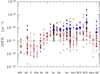Fig. A.1.

Relation between the specific star formation rate and the morphological type for HI-normal (HI-def ≤0.4; filled dots) and HI-deficient (HI-def > 0.4; empty circles) galaxies. The large filled blue dots indicate the mean values for each morphological class for normal gas-rich systems, and the empty red dots show cluster HI-deficient galaxies. The error bar shows the standard deviation of the distribution for the large symbols. The dashed line shows the limit between star-forming and quiescent galaxies.

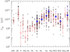Fig. A.2.

Relation between the HI gas depletion timescale and the morphological type for HI-normal (HI-def ≤0.4; filled dots) and HI-deficient (HI-def > 0.4; empty circles) galaxies. The large filled blue dots indicate the mean values for each morphological class for normal gas-rich systems, and the empty red dots show cluster HI-deficient galaxies. The error bar shows the standard deviation of the distribution for the large symbols. Upper limits are indicated by triangles and are treated as detections in the derivation of the mean values.

As expected, Fig. A.1 shows that the activity of star formation per unit stellar mass is significantly higher in spiral galaxies than in Hα detected early-type systems. These early types are just a small fraction of the quiescent galaxy population dominant in the Virgo cluster (Sandage et al. 1985). They are characterised by a residual star formation activity and are probably representative of the population of galaxies at an evolved stage of their transformation from the blue cloud to the red sequence (e.g. Boselli et al. 2014a). The same figure also shows that the specific star formation rate of gas-rich systems of similar morphological type is higher than that of gas-poor objects on average. Finally, despite the much improved quality of the data of the adopted dust attenuation corrections and of the morphological classification, it is clear that the intrinsic scatter within each morphological type is huge also within the unperturbed sample, and it confirms the fact that galaxies of similar morphology undergo very different star formation histories (e.g. Kennicutt et al. 1994). The lack of gas-rich systems with morphological type earlier than Sc and the large fraction of HI undetected systems among the early types hampers the identification of any clear trend between the gas depletion timescale and the morphological type (Fig. A.2). For galaxies of type > Sc, the difference between τ_HI in gas-rich and gas-poor systems is marginal.

Appendix B: Galaxies above the main sequence relation

Figure B.1 shows the continuum-subtracted Hα images of the ten galaxies located more than 1σ above the main-sequence relation and listed in Table 4. In most of them, the star formation activity is dominated by one or a few bright HII regions typical of starbursts. Some of them (VCC 428, VCC 801, and VCC 1554) show filaments or loops of ionised gas escaping from these bright HII regions and extending out of the stellar disc, suggesting the presence of outflows. In others, the asymmetric distribution of the star-forming regions and the tails of ionised gas rather suggest an ongoing ram-pressure-stripping event (VCC 562, AGC224696, and AGC 226326).

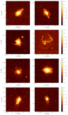Fig. B.1.

Continuum-subtracted Hα images of the galaxies VCC 207, VCC 428, VCC 562, VCC 683, VCC 801, VCC 1313, VCC 1554, and VCC 1744 (from top left to bottom right). The r-band 24 mag arcsec⁻² isophote tracing the distribution of the stellar continuum is overplotted in green.

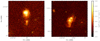Fig. B.2.

Continuum-subtracted Hα images of the galaxies AGC 224696 and AGC 226326 (from left to right). The r-band 24 mag arcsec⁻² isophote tracing the distribution of the stellar continuum is overplotted in green.

All Tables

Table 1.

Multifrequency data.

In the text

Table 2.

Coefficients of the main-sequence relation.

In the text

Table 3.

Average scaling relations.

In the text

Table 4.

Galaxies at more than 1σ above the main sequence.

In the text

All Figures

	Fig. 1. Stellar mass distribution of the Hα detected galaxies (filled red histogram), of the VCC (hatched blue histogram) and of the NGVS galaxies (empty black histogram) classified as Virgo cluster members. Stellar masses are derived as described in Sect. 3.1.
In the text

Fig. 2.

Correction for [NII] contamination. Left panels: relation between the [NII]λ6548 + 6583 Å/Hα line ratio (upper panel), the dust attenuation measured using the Balmer decrement A(Hα)_BD (middle panel), and the dust attenuation A(Hα) derived by averaging the Balmer decrement and the far-infrared determinations (see Sect. 3.3; lower panel) and the stellar mass of the selected galaxies. The long-dashed red lines indicate the mean relations derived in this work. Right panels: [NII]λ6548 + 6583 Å/Hα, A(Hα)_BD, and A(Hα) distributions. The hatched red and blue histograms give the distribution of [NII]λ6548 + 6583 Å/Hα, A(Hα)_BD, and A(Hα) derived from the mean scaling relations given in the text and adopted in the Hα flux correction for galaxies without any spectroscopic data.

In the text

Fig. 3.

Relation between the specific star formation rate and the stellar mass (left) and stellar mass surface density (right) for HI-normal (HI-def ≤ 0.4; filled dots) and HI-deficient (HI-def > 0.4; empty circles) galaxies. The large filled blue dots indicate the mean values for normal gas-rich systems, and the empty red dots show mean values for HI-deficient galaxies. The error bar shows the standard deviation of the distribution for the large symbols. The dashed line shows the limit between star-forming and quiescent galaxies. The typical uncertainty in the data is shown in the lower left corner of each panel.

In the text

Fig. 4.

Relation between the HI gas depletion timescale and stellar mass (left), stellar mass surface density (centre), and specific star formation rate (right) for HI-normal (HI-def ≤ 0.4; filled dots) and HI-deficient (HI-def > 0.4; empty circles) galaxies. The large filled blue dots indicate the mean values for each morphological class for normal gas-rich systems, and the empty red dots show mean values for HI-deficient galaxies. The error bar shows the standard deviation of the distribution for the large symbols. Upper limits are indicated by triangles and are treated as detections in the derivation of the mean values. The dotted line indicates the detection limit of the ALFALFA survey. The typical uncertainty in the data is shown in the lower left corner of each panel.

In the text

Fig. 5.

Main-sequence relation for galaxies in the Virgo cluster coded according to their HI gas content: filled dots show HI gas-rich objects (HI-def ≤ 0.4), and empty circles represent HI-deficient objects (HI-def ≤ 0.4). Large solid blue and empty red circles are the mean values and standard deviations for HI-normal and HI-deficient objects. Star formation rates were derived assuming stationary conditions. The Y-axis on the right side gives the corresponding Hα luminosities corrected for dust attenuation. The solid black line is the best fit; obtained for gas-rich star-forming systems. The best fit is compared to those derived for bright galaxies with HI-def ≤ 0.4 included in the HRS (Boselli et al. 2015, bisector fit) and Speagle et al. (2014, derived extrapolating the time-dependent best-fit relation to z = 0), for the SDSS sample of Peng et al. (2010) derived for galaxies with M_star ≥ 10^8.5 M_⊙, for the local sample of Vilella-Rojo et al. (2021), and for the low surface brightness sample of McGaugh et al. (2017). The typical uncertainty on the data is shown in the lower left corner.

In the text

	Fig. 6. Distribution of the orthogonal distance from the best fit of the main-sequence relation for the whole sample of galaxies (solid black histogram) and for the galaxies with a normal HI gas content (HI-def ≤ 0.4; hatched red histogram).
In the text

Fig. 7.

Main-sequence relation for galaxies coded according to their distance to the best fit derived for HI gas-rich late-type systems. Filled black dots show galaxies within 1σ from the relation, and filled grey dots show galaxies > 1σ above or below the relation. The solid line gives the best fit obtained for gas-rich star-forming systems, and the dotted lines show the limits 1σ above and below the best fit. Galaxies undergoing a ram-pressure-stripping event identified in Boselli et al. (2022a) are indicated with large empty coloured symbols: brown circles show those belonging to the Norma cluster, green squares stand for Coma, and blue hexagons represent A1367. Red triangles indicate the jellyfish sample of Vulcani et al. (2018). Star formation rates and stellar masses are derived consistently with those measured within the Virgo cluster. The typical uncertainty on the data is shown in the lower left corner.

In the text

Fig. 8.

Main-sequence relation for galaxies coded according to their morphological type and HI gas content: Late-type galaxies (≥Sa) are indicated by black symbols, and early-type galaxies are shown by red symbols. Filled dots are for HI gas-rich objects (HI-def ≤ 0.4), and HI-deficient objects (HI-def > 0.4) are shown by empty circles. Star formation rates were derived assuming stationary conditions. The Y-axis on the right side gives the corresponding Hα luminosities corrected for dust attenuation. The solid line is the best fit obtained for gas-rich star-forming systems. The horizontal dotted and dashed lines indicate the corresponding SFR derived using the number of ionising photons produced by an O3 class III and a B0 class III star as derived using the model atmospheres of Sternberg et al. (2003). The typical uncertainty on the data is shown in the lower left corner.

In the text

Fig. 9.

Relation between the offset from the main-sequence relation log SFR/SFR_MS and the HI-deficiency parameter: Late-type galaxies (≥Sa) are indicated by black symbols, early-type galaxies by red symbols, circles stand for HI detected sources, and triangles stand for HI undetected objects (lower limits to the HI-deficiency parameter). Filled symbols show HI gas-rich objects (HI-def ≤ 0.4), and empty symbols show HI-deficient objects (HI-def > 0.4). The data are compared to the predictions of models for starvation (magenta) and ram-pressure stripping (cyan) derived for a galaxy with a rotational velocity 70 km s⁻¹ and spin parameter λ = 0.05. The filled green square indicates the prediction for an unperturbed system. Different symbols in the models indicate the position of the model galaxies at a given look-back time from the beginning of the interaction.

In the text

Fig. 10.

Comparison of the observed main-sequence relation with the predictions of ram-pressure-stripping models for galaxies with a spin parameter λ = 0.05 and rotational velocities of 40, 70, 130, and 220 km s⁻¹. Unperturbed models are indicated with filled green squares, starvation models by the magenta lines, and ram-pressure-stripping models by the cyan lines. Different symbols for the models indicate the position of the model galaxies at a given look-back time from the beginning of the interaction. Black (red) filled circles show late-type (early-type) galaxies with a normal HI content (HI-def ≤ 0.4), and black (red) empty circles show HI-deficient (HI-def > 0.4) late-type (early-type) systems. The typical uncertainty on the data is shown in the lower left corner.

In the text

Fig. 11.

Main-sequence relation for galaxies coded according to their distance from the best fit derived for HI gas-rich late-type systems. Filled black dots show galaxies within 1σ from the relation, and filled grey dots show galaxies > 1σ above or below the relation. The solid line is the best fit obtained for gas-rich star-forming systems, and the dotted lines show the limits 1σ above and below the best fit. Galaxies undergoing a ram-pressure-stripping event identified in Boselli et al. (2022a) are indicated with coloured squares, and those subjected to a combined effect of ram pressure and harassment are shown by triangles. The typical uncertainty on the data is shown in the lower left corner.

In the text

Fig. 12.

Phase-space diagram for the Hα detected galaxies within the Virgo cluster. For all galaxies, the X-axis indicates the projected distance from the central galaxy M87 in units of r₂₀₀, and the Y-axis shows the excess in velocity with respect to the mean velocity of cluster A (⟨v⟩ = 955 km s⁻¹) normalised to its mean velocity dispersion (σ = 799 km s⁻¹; Boselli et al. 2014c). Late-type galaxies (> Sa) are indicated by black symbols, and early-type galaxies are shown by red symbols. Filled dots show HI gas-rich objects (HI-def ≤ 0.4), and HI-deficient objects (HI-def > 0.4) are shown by empty circles. The solid lines delimit the different regions extracted from the simulations of Rhee et al. (2017) to identify galaxies in different phases of their infall into the cluster: first (not yet fallen), recent (0 < τ_inf < 3.6 Gyr), intermediate (3.6 < τ_inf < 6.5 Gyr), and ancient (6.5 < τ_inf < 13.7 Gyr) infallers.

In the text

Fig. 13.

Main-sequence relation for galaxies coded according to their distance from the best fit derived for HI gas-rich late-type systems. Filled black dots show galaxies within 1 σ from the relation, filled blue dots show galaxies > 1σ above the relation, empty black circles show galaxies 1σ–3σ below the relation, and filled red dots show galaxies > 5σ below the relation. The solid line is the best fit obtained for gas-rich star-forming systems. The typical uncertainty on the data is shown in the lower left corner.

In the text

Fig. 14.

Phase–space diagram for galaxies coded according to their distance from the best fit derived for HI gas-rich late-type systems. Filled black dots show galaxies within 1σ from the relation, filled blue dots show galaxies > 1σ above the relation, empty circles show galaxies 1σ–3σ below the relation, and filled dots show galaxies > 5σ below the relation. The solid lines delimit the different regions extracted from the simulations of Rhee et al. (2017) to identify galaxies in different phases of their infall into the cluster: first (not yet fallen), recent (0 < τ_inf < 3.6 Gyr), intermediate (3.6 < τ_inf < 6.5 Gyr), and ancient (6.5 < τ_inf < 13.7 Gyr) infallers.

In the text

Fig. 15.

Phase–space diagram in three different bins of stellar mass (M_star > 10^9.5 M_⊙, massive; 10⁸ < M_star ≤ 10^9.5 M_⊙, intermediate; and M_star ≤ 10⁸ M_⊙, dwarfs) for galaxies coded according to their morphological type (black symbols for late types, and red symbols for early types) and atomic gas content (filled dots for HI gas-rich objects (HI-def ≤ 0.4), and empty circles show HI-deficient objects (HI-def > 0.4)). The solid lines delimit the different regions extracted from the simulations of Rhee et al. (2017) to identify galaxies in different phases of their infall into the cluster: first (not yet fallen), recent (0 < τ_inf < 3.6 Gyr), intermediate (3.6 < τ_inf < 6.5 Gyr), and ancient (6.5 < τ_inf < 13.7 Gyr) infallers.

In the text

Fig. 16.

Phase–space diagram in three different bins of stellar mass (M_star > 10^9.5 M_⊙, massive; 10⁸ < M_star ≤ 10^9.5 M_⊙, intermediate; and M_star ≤ 10⁸ M_⊙, dwarfs) for galaxies coded according to their distance from the main-sequence relation derived for gas-rich late-type systems: filled black dots show galaxies within 1σ from the relation, filled blue dots show galaxies > 1σ above the relation, empty black circles show galaxies 1σ–3σ below the relation, and filled red dots show galaxies > 3σ below the relation. The solid lines delimit the different regions extracted from the simulations of Rhee et al. (2017) to identify galaxies in different phases of their infall into the cluster: first (not yet fallen), recent (0 < τ_inf < 3.6 Gyr), intermediate (3.6 < τ_inf < 6.5 Gyr), and ancient (6.5 < τ_inf < 13.7 Gyr) infallers.

In the text

Fig. 17.

Main-sequence relation including extraplanar HII regions. Left panel: relation between the Hα luminosity (corrected for dust attenuation) and stellar mass for galaxies coded according to their morphological type and HI gas content: late-type galaxies (> Sa) are indicated by black symbols, and early-type galaxies by red symbols. Filled dots show HI gas-rich objects (HI-def ≤ 0.4), and HI-deficient objects (HI-def > 0.4) are shown by empty circles. The solid line is the best fit obtained for gas-rich star-forming systems. Blue triangles show the extraplanar HII regions detected in NGC 4254 (Boselli et al. 2018b), where stellar masses and star formation rates have been determined using the SED fitting code CIGALE. Filled triangles show Hα detected regions, and empty triangles stand for the undetected ones. The error bars of the HII regions of NGC 4254 are those given by the SED fitting analysis. The horizontal dotted and dashed lines indicate the corresponding SFR derived using the number of ionising photons produced by an O3 class III and a B0 class III star as derived using the model atmospheres of Sternberg et al. (2003). The dot-dashed red line indicates the corresponding completeness limit of VESTIGE at the mean distance of Virgo (16.5 Mpc). The right Y-axis gives the corresponding SFR (main-sequence relation) derived assuming stationary conditions. Right panel: similar plot, in which the green filled triangles are the extraplanar HII regions of NGC 4254 detected in Hα, where the stellar masses are derived using the SED fitting analysis with CIGALE, while the star formation rates are measured using the same calibration based on the Hα luminosity as for the galaxy sample, assuming A(Hα) = 0.7 mag and [NII]λ6584 Å/Hα = 0.2, as in Boselli et al. (2018b). The uncertainties on the stellar mass of the HII regions of NGC 4254 are given by the fitting code CIGALE, and those on their star formation rate indicate the dynamic range in this parameter assuming either A(Hα) = 0 mag or A(Hα) = 1.5 mag.

In the text

Fig. A.1.

Relation between the specific star formation rate and the morphological type for HI-normal (HI-def ≤0.4; filled dots) and HI-deficient (HI-def > 0.4; empty circles) galaxies. The large filled blue dots indicate the mean values for each morphological class for normal gas-rich systems, and the empty red dots show cluster HI-deficient galaxies. The error bar shows the standard deviation of the distribution for the large symbols. The dashed line shows the limit between star-forming and quiescent galaxies.

In the text

Fig. A.2.

Relation between the HI gas depletion timescale and the morphological type for HI-normal (HI-def ≤0.4; filled dots) and HI-deficient (HI-def > 0.4; empty circles) galaxies. The large filled blue dots indicate the mean values for each morphological class for normal gas-rich systems, and the empty red dots show cluster HI-deficient galaxies. The error bar shows the standard deviation of the distribution for the large symbols. Upper limits are indicated by triangles and are treated as detections in the derivation of the mean values.

In the text

	Fig. B.1. Continuum-subtracted Hα images of the galaxies VCC 207, VCC 428, VCC 562, VCC 683, VCC 801, VCC 1313, VCC 1554, and VCC 1744 (from top left to bottom right). The r-band 24 mag arcsec⁻² isophote tracing the distribution of the stellar continuum is overplotted in green.
In the text

	Fig. B.2. Continuum-subtracted Hα images of the galaxies AGC 224696 and AGC 226326 (from left to right). The r-band 24 mag arcsec⁻² isophote tracing the distribution of the stellar continuum is overplotted in green.
In the text

Current usage metrics show cumulative count of Article Views (full-text article views including HTML views, PDF and ePub downloads, according to the available data) and Abstracts Views on Vision4Press platform.

Data correspond to usage on the plateform after 2015. The current usage metrics is available 48-96 hours after online publication and is updated daily on week days.

Initial download of the metrics may take a while.

[1] Abadi, M. G., Moore, B., & Bower, R. G. 1999, MNRAS, 308, 947 [Google Scholar]

[2] Abramson, A., & Kenney, J. D. P. 2014, AJ, 147, 63 [Google Scholar]

[3] Abramson, A., Kenney, J. D. P., Crowl, H. H., et al. 2011, AJ, 141, 164 [Google Scholar]

[4] Abramson, A., Kenney, J., Crowl, H., & Tal, T. 2016, AJ, 152, 32 [Google Scholar]

[5] Arrigoni Battaia, F., Gavazzi, G., Fumagalli, M., et al. 2012, A&A, 543, A112 [NASA ADS] [CrossRef] [EDP Sciences] [Google Scholar]

[6] Baldwin, J. A., Phillips, M. M., & Terlevich, R. 1981, PASP, 93, 5 [Google Scholar]

[7] Balogh, M. L., Navarro, J. F., & Morris, S. L. 2000, ApJ, 540, 113 [Google Scholar]

[8] Balogh, M. L., McGee, S. L., Mok, A., et al. 2016, MNRAS, 456, 4364 [NASA ADS] [CrossRef] [Google Scholar]

[9] Bauer, A. E., Hopkins, A. M., Gunawardhana, M., et al. 2013, MNRAS, 434, 209 [NASA ADS] [CrossRef] [Google Scholar]

[10] Bekki, K. 2014, MNRAS, 438, 444 [Google Scholar]

[11] Bekki, K., & Couch, W. J. 2003, ApJ, 596, L13 [NASA ADS] [CrossRef] [Google Scholar]

[12] Belfiore, F., Santoro, F., Groves, B., et al. 2022, A&A, 659, A26 [NASA ADS] [CrossRef] [EDP Sciences] [Google Scholar]

[13] Bigiel, F., Leroy, A., Walter, F., et al. 2008, AJ, 136, 2846 [NASA ADS] [CrossRef] [Google Scholar]

[14] Binggeli, B., Sandage, A., & Tammann, G. A. 1985, AJ, 90, 1681 [Google Scholar]

[15] Boissier, S., & Prantzos, N. 2000, MNRAS, 312, 398 [Google Scholar]

[16] Boissier, S., Prantzos, N., Boselli, A., & Gavazzi, G. 2003, MNRAS, 346, 1215 [NASA ADS] [CrossRef] [Google Scholar]

[17] Boquien, M., Burgarella, D., Roehlly, Y., et al. 2019, A&A, 622, A103 [NASA ADS] [CrossRef] [EDP Sciences] [Google Scholar]

[18] Boselli, A. 2011, A Panchromatic View of Galaxies (Berlin: Wiley-VCH), 324 [Google Scholar]

[19] Boselli, A., & Gavazzi, G. 2006, PASP, 118, 517 [Google Scholar]

[20] Boselli, A., & Gavazzi, G. 2009, A&A, 508, 201 [NASA ADS] [CrossRef] [EDP Sciences] [Google Scholar]

[21] Boselli, A., & Gavazzi, G. 2014, A&ARv, 22, 74 [Google Scholar]

[22] Boselli, A., Gavazzi, G., Donas, J., & Scodeggio, M. 2001, AJ, 121, 753 [NASA ADS] [CrossRef] [Google Scholar]

[23] Boselli, A., Lequeux, J., & Gavazzi, G. 2002, A&A, 384, 33 [NASA ADS] [CrossRef] [EDP Sciences] [Google Scholar]

[24] Boselli, A., Boissier, S., Cortese, L., et al. 2006, ApJ, 651, 811 [Google Scholar]

[25] Boselli, A., Boissier, S., Cortese, L., & Gavazzi, G. 2008a, ApJ, 674, 742 [Google Scholar]

[26] Boselli, A., Boissier, S., Cortese, L., & Gavazzi, G. 2008b, A&A, 489, 1015 [CrossRef] [EDP Sciences] [Google Scholar]

[27] Boselli, A., Boissier, S., Cortese, L., et al. 2009, ApJ, 706, 1527 [Google Scholar]

[28] Boselli, A., Eales, S., Cortese, L., et al. 2010, PASP, 122, 261 [Google Scholar]

[29] Boselli, A., Boissier, S., Heinis, S., et al. 2011, A&A, 528, A107 [NASA ADS] [CrossRef] [EDP Sciences] [Google Scholar]

[30] Boselli, A., Hughes, T. M., Cortese, L., Gavazzi, G., & Buat, V. 2013, A&A, 550, A114 [NASA ADS] [CrossRef] [EDP Sciences] [Google Scholar]

[31] Boselli, A., Cortese, L., Boquien, M., et al. 2014a, A&A, 564, A66 [NASA ADS] [CrossRef] [EDP Sciences] [Google Scholar]

[32] Boselli, A., Cortese, L., Boquien, M., et al. 2014b, A&A, 564, A67 [NASA ADS] [CrossRef] [EDP Sciences] [Google Scholar]

[33] Boselli, A., Voyer, E., Boissier, S., et al. 2014c, A&A, 570, A69 [NASA ADS] [CrossRef] [EDP Sciences] [Google Scholar]

[34] Boselli, A., Fossati, M., Gavazzi, G., et al. 2015, A&A, 579, A102 [NASA ADS] [CrossRef] [EDP Sciences] [Google Scholar]

[35] Boselli, A., Cuillandre, J. C., Fossati, M., et al. 2016a, A&A, 587, A68 [NASA ADS] [CrossRef] [EDP Sciences] [Google Scholar]

[36] Boselli, A., Roehlly, Y., Fossati, M., et al. 2016b, A&A, 596, A11 [NASA ADS] [CrossRef] [EDP Sciences] [Google Scholar]

[37] Boselli, A., Fossati, M., Ferrarese, L., et al. 2018a, A&A, 614, A56 [NASA ADS] [CrossRef] [EDP Sciences] [Google Scholar]

[38] Boselli, A., Fossati, M., Cuillandre, J. C., et al. 2018b, A&A, 615, A114 [NASA ADS] [CrossRef] [EDP Sciences] [Google Scholar]

[39] Boselli, A., Fossati, M., Consolandi, G., et al. 2018c, A&A, 620, A164 [NASA ADS] [CrossRef] [EDP Sciences] [Google Scholar]

[40] Boselli, A., Fossati, M., Longobardi, A., et al. 2019, A&A, 623, A52 [NASA ADS] [CrossRef] [EDP Sciences] [Google Scholar]

[41] Boselli, A., Lupi, A., Epinat, B., et al. 2021, A&A, 646, A139 [NASA ADS] [CrossRef] [EDP Sciences] [Google Scholar]

[42] Boselli, A., Fossati, M., & Sun, M. 2022a, A&ARv, 30, 3 [NASA ADS] [CrossRef] [Google Scholar]

[43] Boselli, A., Fossati, M., Longobardi, A., et al. 2022b, A&A, 659, A46 [NASA ADS] [CrossRef] [EDP Sciences] [Google Scholar]

[44] Bouché, N., Dekel, A., Genzel, R., et al. 2010, ApJ, 718, 1001 [Google Scholar]

[45] Brinchmann, J., Charlot, S., White, S. D. M., et al. 2004, MNRAS, 351, 1151 [Google Scholar]

[46] Brown, T., Wilson, C. D., Zabel, N., et al. 2021, ApJS, 257, 21 [NASA ADS] [CrossRef] [Google Scholar]

[47] Bruzual, G., & Charlot, S. 2003, MNRAS, 344, 1000 [NASA ADS] [CrossRef] [Google Scholar]

[48] Calzetti, D., Kinney, A. L., & Storchi-Bergmann, T. 1994, ApJ, 429, 582 [Google Scholar]

[49] Calzetti, D., Armus, L., Bohlin, R. C., et al. 2000, ApJ, 533, 682 [NASA ADS] [CrossRef] [Google Scholar]

[50] Calzetti, D., Kennicutt, R. C., Engelbracht, C. W., et al. 2007, ApJ, 666, 870 [Google Scholar]

[51] Calzetti, D., Wu, S.-Y., Hong, S., et al. 2010, ApJ, 714, 1256 [Google Scholar]

[52] Caputi, K. I., Deshmukh, S., Ashby, M. L. N., et al. 2017, ApJ, 849, 45 [Google Scholar]

[53] Cardelli, J. A., Clayton, G. C., & Mathis, J. S. 1989, ApJ, 345, 245 [Google Scholar]

[54] Castignani, G., Combes, F., Jablonka, P., et al. 2022, A&A, 657, A9 [NASA ADS] [CrossRef] [EDP Sciences] [Google Scholar]

[55] Cattorini, F., Gavazzi, G., Boselli, A., et al. 2022, A&A, in press [arXiv:2211.06437] [Google Scholar]

[56] Cayatte, V., van Gorkom, J. H., Balkowski, C., & Kotanyi, C. 1990, AJ, 100, 604 [NASA ADS] [CrossRef] [Google Scholar]

[57] Cayatte, V., Kotanyi, C., Balkowski, C., et al. 1994, AJ, 107, 1003 [Google Scholar]

[58] Cerviño, M., & Luridiana, V. 2004, A&A, 413, 145 [NASA ADS] [CrossRef] [EDP Sciences] [Google Scholar]

[59] Cerviño, M., Luridiana, V., Pérez, E., et al. 2003, A&A, 407, 177 [NASA ADS] [CrossRef] [EDP Sciences] [Google Scholar]

[60] Cerviño, M., Román-Zúñiga, C., Luridiana, V., et al. 2013, A&A, 553, A31 [NASA ADS] [CrossRef] [EDP Sciences] [Google Scholar]

[61] Chabrier, G. 2003, PASP, 115, 763 [Google Scholar]

[62] Chevalier, R. A., & Clegg, A. W. 1985, Nature, 317, 44 [Google Scholar]

[63] Chisholm, J., Gazagnes, S., Schaerer, D., et al. 2018, A&A, 616, A30 [NASA ADS] [CrossRef] [EDP Sciences] [Google Scholar]

[64] Choi, Y., Dalcanton, J. J., Williams, B. F., et al. 2020, ApJ, 902, 54 [NASA ADS] [CrossRef] [Google Scholar]

[65] Chung, A., van Gorkom, J. H., Kenney, J. D. P., & Vollmer, B. 2007, ApJ, 659, L115 [Google Scholar]

[66] Chung, A., van Gorkom, J. H., Kenney, J. D. P., Crowl, H., & Vollmer, B. 2009, AJ, 138, 1741 [Google Scholar]

[67] Cid Fernandes, R., Stasińska, G., Mateus, A., et al. 2011, MNRAS, 413, 1687 [NASA ADS] [CrossRef] [Google Scholar]

[68] Ciesla, L., Boquien, M., Boselli, A., et al. 2014, A&A, 565, A128 [NASA ADS] [CrossRef] [EDP Sciences] [Google Scholar]

[69] Ciesla, L., Buat, V., Boquien, M., et al. 2021, A&A, 653, A6 [NASA ADS] [CrossRef] [EDP Sciences] [Google Scholar]

[70] Cole, S., Aragon-Salamanca, A., Frenk, C. S., et al. 1994, MNRAS, 271, 781 [NASA ADS] [CrossRef] [Google Scholar]

[71] Conroy, C. 2013, ARA&A, 51, 393 [NASA ADS] [CrossRef] [Google Scholar]

[72] Conroy, C., Gunn, J. E., & White, M. 2009, ApJ, 699, 486 [Google Scholar]

[73] Cortese, L., Davies, J. I., Pohlen, M., et al. 2010, A&A, 518, L49 [NASA ADS] [CrossRef] [EDP Sciences] [Google Scholar]

[74] Cortese, L., Fritz, J., Bianchi, S., et al. 2014, MNRAS, 440, 942 [Google Scholar]

[75] Cortese, L., Catinella, B., & Smith, R. 2021, PASA, 38, e035 [NASA ADS] [CrossRef] [Google Scholar]

[76] Cowie, L. L., Songaila, A., Hu, E. M., & Cohen, J. G. 1996, AJ, 112, 839 [Google Scholar]

[77] Cramer, W. J., Kenney, J. D. P., Sun, M., et al. 2019, ApJ, 870, 63 [Google Scholar]

[78] Cramer, W. J., Kenney, J. D. P., Cortes, J. R., et al. 2020, ApJ, 901, 95 [NASA ADS] [CrossRef] [Google Scholar]

[79] Crowl, H. H., & Kenney, J. D. P. 2008, AJ, 136, 1623 [Google Scholar]

[80] Crowl, H. H., Kenney, J. D. P., van Gorkom, J. H., & Vollmer, B. 2005, AJ, 130, 65 [Google Scholar]

[81] Cybulski, R., Yun, M. S., Fazio, G. G., et al. 2014, MNRAS, 439, 3564 [NASA ADS] [CrossRef] [Google Scholar]

[82] Daddi, E., Dickinson, M., Morrison, G., et al. 2007, ApJ, 670, 156 [NASA ADS] [CrossRef] [Google Scholar]

[83] Dale, D. A., Helou, G., Magdis, G. E., et al. 2014, ApJ, 784, 83 [Google Scholar]

[84] da Silva, R. L., Fumagalli, M., & Krumholz, M. 2012, ApJ, 745, 145 [CrossRef] [Google Scholar]

[85] da Silva, R. L., Fumagalli, M., & Krumholz, M. R. 2014, MNRAS, 444, 3275 [Google Scholar]

[86] Davies, J. I., Baes, M., Bendo, G. J., et al. 2010, A&A, 518, L48 [NASA ADS] [CrossRef] [EDP Sciences] [Google Scholar]

[87] De Lucia, G., Weinmann, S., Poggianti, B. M., Aragón-Salamanca, A., & Zaritsky, D. 2012, MNRAS, 423, 1277 [NASA ADS] [CrossRef] [Google Scholar]

[88] Domainko, W., Mair, M., Kapferer, W., et al. 2006, A&A, 452, 795 [NASA ADS] [CrossRef] [EDP Sciences] [Google Scholar]

[89] Donnari, M., Pillepich, A., Nelson, D., et al. 2019, MNRAS, 485, 4817 [Google Scholar]

[90] Dressler, A. 1980, ApJ, 236, 351 [Google Scholar]

[91] Dressler, A. 2004, Clusters of Galaxies: Probes of Cosmological Structure and Galaxy Evolution (Cambridge: Cambridge University Press), 206 [Google Scholar]

[92] Duc, P.-A., & Bournaud, F. 2008, ApJ, 673, 787 [NASA ADS] [CrossRef] [Google Scholar]

[93] Elbaz, D., Daddi, E., Le Borgne, D., et al. 2007, A&A, 468, 33 [NASA ADS] [CrossRef] [EDP Sciences] [Google Scholar]

[94] Elmegreen, B. G. 2000, ApJ, 539, 342 [NASA ADS] [CrossRef] [Google Scholar]

[95] Emami, N., Siana, B., Weisz, D. R., et al. 2019, ApJ, 881, 71 [NASA ADS] [CrossRef] [Google Scholar]

[96] Erfanianfar, G., Popesso, P., Finoguenov, A., et al. 2016, MNRAS, 455, 2839 [NASA ADS] [CrossRef] [Google Scholar]

[97] Ferrarese, L., Côté, P., Cuillandre, J.-C., et al. 2012, ApJS, 200, 4 [Google Scholar]

[98] Ferrarese, L., Côté, P., MacArthur, L. A., et al. 2020, ApJ, 890, 128 [Google Scholar]

[99] Filho, M. E., Sánchez Almeida, J., Amorín, R., et al. 2016, ApJ, 820, 109 [NASA ADS] [CrossRef] [Google Scholar]

[100] Flores Velázquez, J. A., Gurvich, A. B., Faucher-Giguère, C.-A., et al. 2021, MNRAS, 501, 4812 [CrossRef] [Google Scholar]

[101] Fossati, M., Gavazzi, G., Savorgnan, G., et al. 2013, A&A, 553, A91 [NASA ADS] [CrossRef] [EDP Sciences] [Google Scholar]

[102] Fossati, M., Mendel, J. T., Boselli, A., et al. 2018, A&A, 614, A57 [NASA ADS] [CrossRef] [EDP Sciences] [Google Scholar]

[103] Fujita, Y. 2004, PASJ, 56, 29 [NASA ADS] [Google Scholar]

[104] Fujita, Y., & Nagashima, M. 1999, ApJ, 516, 619 [NASA ADS] [CrossRef] [Google Scholar]

[105] Fumagalli, M., Krumholz, M. R., Prochaska, J. X., et al. 2009, ApJ, 697, 1811 [NASA ADS] [CrossRef] [Google Scholar]

[106] Fumagalli, M., da Silva, R. L., & Krumholz, M. R. 2011a, ApJ, 741, L26 [NASA ADS] [CrossRef] [Google Scholar]

[107] Fumagalli, M., Gavazzi, G., Scaramella, R., & Franzetti, P. 2011b, A&A, 528, A46 [NASA ADS] [CrossRef] [EDP Sciences] [Google Scholar]

[108] Gardan, E., Braine, J., Schuster, K. F., et al. 2007, A&A, 473, 91 [NASA ADS] [CrossRef] [EDP Sciences] [Google Scholar]

[109] Gavazzi, G., & Boselli, A. 1999a, A&A, 343, 86 [NASA ADS] [Google Scholar]

[110] Gavazzi, G., & Boselli, A. 1999b, A&A, 343, 93 [NASA ADS] [Google Scholar]

[111] Gavazzi, G., Contursi, A., Carrasco, L., et al. 1995, A&A, 304, 325 [NASA ADS] [Google Scholar]

[112] Gavazzi, G., Pierini, D., & Boselli, A. 1996, A&A, 312, 397 [NASA ADS] [Google Scholar]

[113] Gavazzi, G., Catinella, B., Carrasco, L., Boselli, A., & Contursi, A. 1998, AJ, 115, 1745 [NASA ADS] [CrossRef] [Google Scholar]

[114] Gavazzi, G., Boselli, A., Scodeggio, M., Pierini, D., & Belsole, E. 1999, MNRAS, 304, 595 [Google Scholar]

[115] Gavazzi, G., Boselli, A., Vílchez, J. M., Iglesias-Paramo, J., & Bonfanti, C. 2000, A&A, 361, 1 [NASA ADS] [Google Scholar]

[116] Gavazzi, G., Boselli, A., Mayer, L., et al. 2001, ApJ, 563, L23 [Google Scholar]

[117] Gavazzi, G., Boselli, A., Pedotti, P., Gallazzi, A., & Carrasco, L. 2002, A&A, 396, 449 [NASA ADS] [CrossRef] [EDP Sciences] [Google Scholar]

[118] Gavazzi, G., Boselli, A., Donati, A., Franzetti, P., & Scodeggio, M. 2003, A&A, 400, 451 [NASA ADS] [CrossRef] [EDP Sciences] [Google Scholar]

[119] Gavazzi, G., Zaccardo, A., Sanvito, G., Boselli, A., & Bonfanti, C. 2004, A&A, 417, 499 [NASA ADS] [CrossRef] [EDP Sciences] [Google Scholar]

[120] Gavazzi, G., Boselli, A., van Driel, W., & O’Neil, K. 2005, A&A, 429, 439 [NASA ADS] [CrossRef] [EDP Sciences] [Google Scholar]

[121] Gavazzi, G., Boselli, A., Cortese, L., et al. 2006a, A&A, 446, 839 [NASA ADS] [CrossRef] [EDP Sciences] [Google Scholar]

[122] Gavazzi, G., O’Neil, K., Boselli, A., & van Driel, W. 2006b, A&A, 449, 929 [NASA ADS] [CrossRef] [EDP Sciences] [Google Scholar]

[123] Gavazzi, G., Fumagalli, M., Cucciati, O., et al. 2010, A&A, 517, A73 [NASA ADS] [CrossRef] [EDP Sciences] [Google Scholar]

[124] Gavazzi, G., Fumagalli, M., Fossati, M., et al. 2013, A&A, 553, A89 [NASA ADS] [CrossRef] [EDP Sciences] [Google Scholar]

[125] Gavazzi, G., Consolandi, G., Dotti, M., et al. 2015, A&A, 580, A116 [NASA ADS] [CrossRef] [EDP Sciences] [Google Scholar]

[126] Gavazzi, G., Consolandi, G., Pedraglio, S., et al. 2018a, A&A, 611, A28 [NASA ADS] [CrossRef] [EDP Sciences] [Google Scholar]

[127] Gavazzi, G., Consolandi, G., Gutierrez, M. L., et al. 2018b, A&A, 618, A130 [NASA ADS] [CrossRef] [EDP Sciences] [Google Scholar]

[128] Giovanelli, R., Haynes, M. P., Kent, B. R., et al. 2005, AJ, 130, 2598 [Google Scholar]

[129] Gunn, J. E., & Gott, J. R., III 1972, ApJ, 176, 1 [Google Scholar]

[130] Gwyn, S. D. J. 2008, PASP, 120, 212 [Google Scholar]

[131] Haines, C. P., Pereira, M. J., Smith, G. P., et al. 2015, ApJ, 806, 101 [NASA ADS] [CrossRef] [Google Scholar]

[132] Haynes, M. P., & Giovanelli, R. 1984, AJ, 89, 758 [Google Scholar]

[133] Haynes, M. P., Giovanelli, R., Kent, B. R., et al. 2018, ApJ, 861, 49 [Google Scholar]

[134] Henderson, B., & Bekki, K. 2016, ApJ, 822, L33 [Google Scholar]

[135] Hester, J. A. 2006, ApJ, 647, 910 [Google Scholar]

[136] Hester, J. A., Seibert, M., Neill, J. D., et al. 2010, ApJ, 716, L14 [Google Scholar]

[137] Hota, A., Devaraj, A., Pradhan, A. C., et al. 2021, JApA, 42, 86 [NASA ADS] [Google Scholar]

[138] Hunt, L. K., De Looze, I., Boquien, M., et al. 2019, A&A, 621, A51 [NASA ADS] [CrossRef] [EDP Sciences] [Google Scholar]

[139] Ilbert, O., McCracken, H. J., Le Fèvre, O., et al. 2013, A&A, 556, A55 [NASA ADS] [CrossRef] [EDP Sciences] [Google Scholar]

[140] Ilbert, O., Arnouts, S., Le Floc’h, E., et al. 2015, A&A, 579, A2 [NASA ADS] [CrossRef] [EDP Sciences] [Google Scholar]

[141] Izotov, Y. I., Schaerer, D., Thuan, T. X., et al. 2016, MNRAS, 461, 3683 [Google Scholar]

[142] Jáchym, P., Combes, F., Cortese, L., Sun, M., & Kenney, J. D. P. 2014, ApJ, 792, 11 [Google Scholar]

[143] Jaffé, Y. L., Smith, R., Candlish, G. N., et al. 2015, MNRAS, 448, 1715 [Google Scholar]

[144] Jaffé, Y. L., Poggianti, B. M., Moretti, A., et al. 2018, MNRAS, 476, 4753 [Google Scholar]

[145] Junais, Boissier S., Boselli, A., et al. 2021, A&A, 650, A99 [NASA ADS] [CrossRef] [EDP Sciences] [Google Scholar]

[146] Junais, Boissier S., Boselli, A., et al. 2022, A&A, 667, A76 [NASA ADS] [CrossRef] [EDP Sciences] [Google Scholar]

[147] Kauffmann, G., White, S. D. M., & Guiderdoni, B. 1993, MNRAS, 264, 201 [Google Scholar]

[148] Kelly, B. C. 2007, ApJ, 665, 1489 [Google Scholar]

[149] Kenney, J. D. P., van Gorkom, J. H., & Vollmer, B. 2004, AJ, 127, 3361 [Google Scholar]

[150] Kenney, J. D. P., Geha, M., Jáchym, P., et al. 2014, ApJ, 780, 119 [Google Scholar]

[151] Kennicutt, R. C. 1989, ApJ, 344, 685 [Google Scholar]

[152] Kennicutt, R. C. 1990, The Interstellar Medium in Galaxies (Dordrecht: Kluwer), 161, 405 [NASA ADS] [CrossRef] [Google Scholar]

[153] Kennicutt, R. C., Jr 1998a, ARA&A, 36, 189 [NASA ADS] [CrossRef] [Google Scholar]

[154] Kennicutt, R. C. 1998b, ApJ, 498, 541 [NASA ADS] [CrossRef] [Google Scholar]

[155] Kennicutt, R. C., Tamblyn, P., & Congdon, C. E. 1994, ApJ, 435, 22 [NASA ADS] [CrossRef] [Google Scholar]

[156] Kennicutt, R. C., Jr, Hao, C.-N., Calzetti, D., et al. 2009, ApJ, 703, 1672 [NASA ADS] [CrossRef] [Google Scholar]

[157] Kim, S., Rey, S.-C., Jerjen, H., et al. 2014, ApJS, 215, 22 [Google Scholar]

[158] Koda, J., Yagi, M., Boissier, S., et al. 2012, ApJ, 749, 20 [NASA ADS] [CrossRef] [Google Scholar]

[159] Koopmann, R. A., & Kenney, J. D. P. 2004a, ApJ, 613, 851 [NASA ADS] [CrossRef] [Google Scholar]

[160] Koopmann, R. A., & Kenney, J. D. P. 2004b, ApJ, 613, 866 [Google Scholar]

[161] Koopmann, R. A., Haynes, M. P., & Catinella, B. 2006, AJ, 131, 716 [NASA ADS] [CrossRef] [Google Scholar]

[162] Koyama, Y., Smail, I., Kurk, J., et al. 2013, MNRAS, 434, 423 [CrossRef] [Google Scholar]

[163] Larson, R. B., Tinsley, B. M., & Caldwell, C. N. 1980, ApJ, 237, 692 [Google Scholar]

[164] Lee, J. H., Hwang, N., & Lee, M. G. 2011, ApJ, 735, 75 [Google Scholar]

[165] Lee, J. H., Kimm, T., Katz, H., et al. 2020, ApJ, 905, 31 [NASA ADS] [CrossRef] [Google Scholar]

[166] Leitherer, C., Hernandez, S., Lee, J. C., et al. 2016, ApJ, 823, 64 [NASA ADS] [CrossRef] [Google Scholar]

[167] Leroy, A. K., Walter, F., Brinks, E., et al. 2008, AJ, 136, 2782 [Google Scholar]

[168] Leroy, A. K., Walter, F., Sandstrom, K., et al. 2013, AJ, 146, 19 [Google Scholar]

[169] Lilly, S. J., Carollo, C. M., Pipino, A., et al. 2013, ApJ, 772, 119 [NASA ADS] [CrossRef] [Google Scholar]

[170] Lim, S., Côté, P., Peng, E. W., et al. 2020, ApJ, 899, 69 [CrossRef] [Google Scholar]

[171] Lin, L., Jian, H.-Y., Foucaud, S., et al. 2014, ApJ, 782, 33 [NASA ADS] [CrossRef] [Google Scholar]

[172] Liu, C., Côté, P., Peng, E. W., et al. 2020, ApJS, 250, 17 [NASA ADS] [CrossRef] [Google Scholar]

[173] Longobardi, A., Boselli, A., Fossati, M., et al. 2020, A&A, 644, A161 [EDP Sciences] [Google Scholar]

[174] Mahajan, S., Mamon, G. A., & Raychaudhury, S. 2011, MNRAS, 416, 2882 [NASA ADS] [CrossRef] [Google Scholar]

[175] Matthee, J., & Schaye, J. 2019, MNRAS, 484, 915 [CrossRef] [Google Scholar]

[176] McGaugh, S. S., Schombert, J. M., & Lelli, F. 2017, ApJ, 851, 22 [Google Scholar]

[177] McGee, S. L., Balogh, M. L., Bower, R. G., Font, A. S., & McCarthy, I. G. 2009, MNRAS, 400, 937 [Google Scholar]

[178] McGee, S. L., Bower, R. G., & Balogh, M. L. 2014, MNRAS, 442, L105 [Google Scholar]

[179] Mei, S., Blakeslee, J. P., Côté, P., et al. 2007, ApJ, 655, 144 [Google Scholar]

[180] Mo, H. J., Mao, S., & White, S. D. M. 1998, MNRAS, 295, 319 [Google Scholar]

[181] Mok, A., Wilson, C. D., Knapen, J. H., et al. 2017, MNRAS, 467, 4282 [NASA ADS] [CrossRef] [Google Scholar]

[182] Moore, B., Lake, G., & Katz, N. 1998, ApJ, 495, 139 [Google Scholar]

[183] Morokuma-Matsui, K., Kodama, T., Morokuma, T., et al. 2021, ApJ, 914, 145 [NASA ADS] [CrossRef] [Google Scholar]

[184] Muñoz-Mateos, J. C., Boissier, S., Gil de Paz, A., et al. 2011, ApJ, 731, 10 [CrossRef] [Google Scholar]

[185] Mutchler, M., Bond, H. E., Christian, C. A., et al. 2007, PASP, 119, 1 [NASA ADS] [CrossRef] [Google Scholar]

[186] Nantais, J., Wilson, G., Muzzin, A., et al. 2020, MNRAS, 499, 3061 [Google Scholar]

[187] Noeske, K. G., Weiner, B. J., Faber, S. M., et al. 2007, ApJ, 660, L43 [CrossRef] [Google Scholar]

[188] Oey, M. S., Meurer, G. R., Yelda, S., et al. 2007, ApJ, 661, 801 [NASA ADS] [CrossRef] [Google Scholar]

[189] Old, L. J., Balogh, M. L., van der Burg, R. F. J., et al. 2020, MNRAS, 493, 5987 [NASA ADS] [CrossRef] [Google Scholar]

[190] Paccagnella, A., Vulcani, B., Poggianti, B. M., et al. 2016, ApJ, 816, L25 [NASA ADS] [CrossRef] [Google Scholar]

[191] Pappalardo, C., Lançon, A., Vollmer, B., et al. 2010, A&A, 514, A33 [NASA ADS] [CrossRef] [EDP Sciences] [Google Scholar]

[192] Pearson, W. J., Wang, L., Hurley, P. D., et al. 2018, A&A, 615, A146 [NASA ADS] [CrossRef] [EDP Sciences] [Google Scholar]

[193] Pedrini, A., Fossati, M., Gavazzi, G., et al. 2022, MNRAS, 511, 5180 [NASA ADS] [CrossRef] [Google Scholar]

[194] Peng, Y.-J., Lilly, S. J., Kovač, K., et al. 2010, ApJ, 721, 193 [Google Scholar]

[195] Pillepich, A., Nelson, D., Springel, V., et al. 2019, MNRAS, 490, 3196 [Google Scholar]

[196] Poggianti, B. M., Moretti, A., Gullieuszik, M., et al. 2017, ApJ, 844, 48 [Google Scholar]

[197] Popesso, P., Concas, A., Morselli, L., et al. 2019, MNRAS, 483, 3213 [Google Scholar]

[198] Popesso, P., Concas, A., Cresci, G., et al. 2022, MNRAS, stac3214 [Google Scholar]

[199] Prantzos, N., & Boissier, S. 2000, MNRAS, 313, 338 [NASA ADS] [CrossRef] [Google Scholar]

[200] Quilis, V., Moore, B., & Bower, R. 2000, Science, 288, 1617 [Google Scholar]

[201] Rhee, J., Smith, R., Choi, H., et al. 2017, ApJ, 843, 128 [Google Scholar]

[202] Rhee, J., Smith, R., Choi, H., et al. 2020, ApJS, 247, 45 [NASA ADS] [CrossRef] [Google Scholar]

[203] Roberts, M. S. 1963, ARA&A, 1, 149 [NASA ADS] [CrossRef] [Google Scholar]

[204] Roberts, M. S., & Haynes, M. P. 1994, ARA&A, 32, 115 [NASA ADS] [CrossRef] [Google Scholar]

[205] Rodighiero, G., Daddi, E., Baronchelli, I., et al. 2011, ApJ, 739, L40 [Google Scholar]

[206] Roediger, E., & Hensler, G. 2005, A&A, 433, 875 [NASA ADS] [CrossRef] [EDP Sciences] [Google Scholar]

[207] Roediger, E., & Brüggen, M. 2006, MNRAS, 369, 567 [NASA ADS] [CrossRef] [Google Scholar]

[208] Roediger, E., & Brüggen, M. 2007, MNRAS, 380, 1399 [Google Scholar]

[209] Roychowdhury, S., Chengalur, J. N., Begum, A., et al. 2009, MNRAS, 397, 1435 [NASA ADS] [CrossRef] [Google Scholar]

[210] Roychowdhury, S., Chengalur, J. N., Kaisin, S. S., et al. 2014, MNRAS, 445, 1392 [NASA ADS] [CrossRef] [Google Scholar]

[211] Sandage, A. 1986, A&A, 161, 89 [NASA ADS] [Google Scholar]

[212] Sandage, A., Binggeli, B., & Tammann, G. A. 1985, AJ, 90, 1759 [NASA ADS] [CrossRef] [Google Scholar]

[213] Sargent, M. T., Béthermin, M., Daddi, E., et al. 2012, ApJ, 747, L31 [NASA ADS] [CrossRef] [Google Scholar]

[214] Schlegel, D. J., Finkbeiner, D. P., & Davis, M. 1998, ApJ, 500, 525 [Google Scholar]

[215] Schreiber, C., Pannella, M., Elbaz, D., et al. 2015, A&A, 575, A74 [NASA ADS] [CrossRef] [EDP Sciences] [Google Scholar]

[216] Semenov, V. A., Kravtsov, A. V., & Gnedin, N. Y. 2017, ApJ, 845, 133 [NASA ADS] [CrossRef] [Google Scholar]

[217] Serra, P., Oosterloo, T., Morganti, R., et al. 2012, MNRAS, 422, 1835 [Google Scholar]

[218] Shopbell, P. L., & Bland-Hawthorn, J. 1998, ApJ, 493, 129 [NASA ADS] [CrossRef] [Google Scholar]

[219] Solanes, J. M., Giovanelli, R., & Haynes, M. P. 1996, ApJ, 461, 609 [Google Scholar]

[220] Solanes, J. M., Manrique, A., García-Gómez, C., et al. 2001, ApJ, 548, 97 [Google Scholar]

[221] Sorce, J. G., Dubois, Y., Blaizot, J., et al. 2021, MNRAS, 504, 2998 [NASA ADS] [CrossRef] [Google Scholar]

[222] Sorgho, A., Hess, K., Carignan, C., et al. 2017, MNRAS, 464, 530 [NASA ADS] [CrossRef] [Google Scholar]

[223] Sparre, M., Hayward, C. C., Springel, V., et al. 2015, MNRAS, 447, 3548 [Google Scholar]

[224] Speagle, J. S., Steinhardt, C. L., Capak, P. L., et al. 2014, ApJS, 214, 15 [NASA ADS] [CrossRef] [Google Scholar]

[225] Steinhauser, D., Haider, M., Kapferer, W., et al. 2012, A&A, 544, A54 [NASA ADS] [CrossRef] [EDP Sciences] [Google Scholar]

[226] Steinhauser, D., Schindler, S., & Springel, V. 2016, A&A, 591, A51 [NASA ADS] [CrossRef] [EDP Sciences] [Google Scholar]

[227] Sternberg, A., Hoffmann, T. L., & Pauldrach, A. W. A. 2003, ApJ, 599, 1333 [NASA ADS] [CrossRef] [Google Scholar]

[228] Steyrleithner, P., Hensler, G., & Boselli, A. 2020, MNRAS, 494, 1114 [Google Scholar]

[229] Sun, M., Donahue, M., & Voit, G. M. 2007, ApJ, 671, 190 [Google Scholar]

[230] Taranu, D. S., Hudson, M. J., Balogh, M. L., et al. 2014, MNRAS, 440, 1934 [Google Scholar]

[231] Tasca, L. A. M., Le Fèvre, O., Hathi, N. P., et al. 2015, A&A, 581, A54 [NASA ADS] [CrossRef] [EDP Sciences] [Google Scholar]

[232] Tran, K.-V. H., Papovich, C., Saintonge, A., et al. 2010, ApJ, 719, L126 [CrossRef] [Google Scholar]

[233] Tran, K.-V. H., Alcorn, L. Y., Kacprzak, G. G., et al. 2017, ApJ, 834, 101 [NASA ADS] [CrossRef] [Google Scholar]

[234] Treu, T., Ellis, R. S., Kneib, J. -P., et al. 2003, ApJ, 591, 53 [NASA ADS] [CrossRef] [Google Scholar]

[235] Troncoso-Iribarren, P., Padilla, N., Santander, C., et al. 2020, MNRAS, 497, 4145 [Google Scholar]

[236] Trussler, J., Maiolino, R., Maraston, C., et al. 2020, MNRAS, 491, 5406 [Google Scholar]

[237] Tyler, K. D., Rieke, G. H., & Bai, L. 2013, ApJ, 773, 86 [NASA ADS] [CrossRef] [Google Scholar]

[238] Tyler, K. D., Bai, L., & Rieke, G. H. 2014, ApJ, 794, 31 [NASA ADS] [CrossRef] [Google Scholar]

[239] Vilella-Rojo, G., Logroño-García, R., López-Sanjuan, C., et al. 2021, A&A, 650, A68 [NASA ADS] [CrossRef] [EDP Sciences] [Google Scholar]

[240] Vollmer, B. 2003, A&A, 398, 525 [NASA ADS] [CrossRef] [EDP Sciences] [Google Scholar]

[241] Vollmer, B. 2009, A&A, 502, 427 [NASA ADS] [CrossRef] [EDP Sciences] [Google Scholar]

[242] Vollmer, B., Cayatte, V., Boselli, A., Balkowski, C., & Duschl, W. J. 1999, A&A, 349, 411 [NASA ADS] [Google Scholar]

[243] Vollmer, B., Marcelin, M., Amram, P., et al. 2000, A&A, 364, 532 [NASA ADS] [Google Scholar]

[244] Vollmer, B., Braine, J., Balkowski, C., et al. 2001a, A&A, 374, 824 [NASA ADS] [CrossRef] [EDP Sciences] [Google Scholar]

[245] Vollmer, B., Cayatte, V., Balkowski, C., & Duschl, W. J. 2001b, ApJ, 561, 708 [NASA ADS] [CrossRef] [Google Scholar]

[246] Vollmer, B., Balkowski, C., Cayatte, V., van Driel, W., & Huchtmeier, W. 2004a, A&A, 419, 35 [CrossRef] [EDP Sciences] [Google Scholar]

[247] Vollmer, B., Beck, R., Kenney, J. D. P., et al. 2004b, AJ, 127, 3375 [Google Scholar]

[248] Vollmer, B., Huchtmeier, W., & van Driel, W. 2005, A&A, 439, 921 [NASA ADS] [CrossRef] [EDP Sciences] [Google Scholar]

[249] Vollmer, B., Soida, M., Otmianowska-Mazur, K., et al. 2006, A&A, 453, 883 [NASA ADS] [CrossRef] [EDP Sciences] [Google Scholar]

[250] Vollmer, B., Soida, M., Chung, A., et al. 2008a, A&A, 483, 89 [NASA ADS] [CrossRef] [EDP Sciences] [Google Scholar]

[251] Vollmer, B., Braine, J., Pappalardo, C., & Hily-Blant, P. 2008b, A&A, 491, 455 [NASA ADS] [CrossRef] [EDP Sciences] [Google Scholar]

[252] Vollmer, B., Soida, M., Braine, J., et al. 2012, A&A, 537, A143 [NASA ADS] [CrossRef] [EDP Sciences] [Google Scholar]

[253] Vollmer, B., Pappalardo, C., Soida, M., et al. 2018, A&A, 620, A108 [NASA ADS] [CrossRef] [EDP Sciences] [Google Scholar]

[254] Vollmer, B., Fossati, M., Boselli, A., et al. 2021, A&A, 645, A121 [EDP Sciences] [Google Scholar]

[255] von der Linden, A., Wild, V., Kauffmann, G., et al. 2010, MNRAS, 404, 1231 [NASA ADS] [Google Scholar]

[256] Vulcani, B., Poggianti, B. M., Finn, R. A., et al. 2010, ApJ, 710, L1 [NASA ADS] [CrossRef] [Google Scholar]

[257] Vulcani, B., Poggianti, B. M., Gullieuszik, M., et al. 2018, ApJ, 866, L25 [Google Scholar]

[258] Yagi, M., Yoshida, M., Komiyama, Y., et al. 2010, AJ, 140, 1814 [Google Scholar]

[259] Yagi, M., Yoshida, M., Gavazzi, G., et al. 2017, ApJ, 839, 65 [NASA ADS] [CrossRef] [Google Scholar]

[260] Yoon, H., Chung, A., Smith, R., et al. 2017, ApJ, 838, 81 [CrossRef] [Google Scholar]

[261] Yoshida, M., Yagi, M., Okamura, S., et al. 2002, ApJ, 567, 118 [NASA ADS] [CrossRef] [Google Scholar]

[262] Yoshida, M., Ohyama, Y., Iye, M., et al. 2004, AJ, 127, 90 [Google Scholar]

[263] Wang, L., Norberg, P., Brough, S., et al. 2018, A&A, 618, A1 [NASA ADS] [CrossRef] [EDP Sciences] [Google Scholar]

[264] Warmels, R. H. 1986, Ph.D. thesis, University of Groningen, The Netherlands [Google Scholar]

[265] Wheeler, C., Phillips, J. I., Cooper, M. C., et al. 2014, MNRAS, 442, 1396 [NASA ADS] [CrossRef] [Google Scholar]

[266] Whitaker, K. E., van Dokkum, P. G., Brammer, G., et al. 2012, ApJ, 754, L29 [NASA ADS] [CrossRef] [Google Scholar]

[267] Whitaker, K. E., Franx, M., Leja, J., et al. 2014, ApJ, 795, 104 [NASA ADS] [CrossRef] [Google Scholar]

[268] Whitmore, B. C., Gilmore, D. M., & Jones, C. 1993, ApJ, 407, 489 [NASA ADS] [CrossRef] [Google Scholar]

[269] Wolf, C., Aragón-Salamanca, A., Balogh, M., et al. 2009, MNRAS, 393, 1302 [Google Scholar]

[270] Wong, T., & Blitz, L. 2002, ApJ, 569, 157 [CrossRef] [Google Scholar]