| Issue |
A&A
Volume 667, November 2022
|
|
|---|---|---|
| Article Number | A117 | |
| Number of page(s) | 25 | |
| Section | Extragalactic astronomy | |
| DOI | https://doi.org/10.1051/0004-6361/202244364 | |
| Published online | 15 November 2022 | |
Properties of the interstellar medium in star-forming galaxies at redshifts 2 ≤ z ≤ 5 from the VANDELS survey
1
INAF – Osservatorio Astronomico di Roma, via di Frascati 33, 00078 Monte Porzio Catone, Italy
e-mail: This email address is being protected from spambots. You need JavaScript enabled to view it.
2
INAF – Osservatorio Astronomico di Bologna, via P. Gobetti 93/3, 40129 Bologna, Italy
3
University of Bologna – Department of Physics and Astronomy ‘Augusto Righi’ (DIFA), via Gobetti 93/2, 40129 Bologna, Italy
4
INAF – Osservatorio Astrofisico di Arcetri, Largo E. Fermi 5, 50125 Firenze, Italy
5
Instituto de Investigación Multidisciplinar en Ciencia y Tecnología, Universidad de La Serena, Raúl Bitrán 1305, La Serena, Chile
6
Departamento de Física y Astronomía, Universidad de La Serena, Av. Juan Cisternas 1200 Norte, La Serena, Chile
7
Cosmic Dawn Center (DAWN), Niels Bohr Institute, University of Copenhagen, Jagtvej 128, 2200 Copenhagen Ø, Denmark
8
European Southern Observatory, Karl Schwarzschild Straße 2, 85748 Garching, Germany
9
Departamento de Ciencias Fisicas, Universidad Andres Bello, Fernandez Concha 700, Las Condes, Santiago, Chile
10
Space Telescope Science Institute, 3700 San Martin Drive, Baltimore, MD 21218, USA
11
Department of Physics and Astronomy, University College London, Gower Street, London WC1E 6BT, UK
12
Department of Astronomy, University of Geneva, 51 Chemin Pegasi, 1290 Versoix, Switzerland
Received:
27
June
2022
Accepted:
19
August
2022
Abstract
Gaseous flows inside and outside galaxies are key to understanding galaxy evolution, as they regulate their star formation activity and chemical enrichment across cosmic time. We study the interstellar medium (ISM) kinematics of a sample of 330 galaxies with C III] or He II emission using far-ultraviolet (far-UV) ISM absorption lines detected in the ultra deep spectra of the VANDELS survey. These galaxies span a broad range of stellar masses from 108 to 1011 M⊙, and star formation rates (SFRs) from 1 to 500 M⊙ yr−1 in the redshift range between 2 and 5. We find that the bulk ISM velocity along the line of sight (vIS) is globally in outflow, with a vIS of −60 ± 10 km s−1 for low-ionisation gas traced by Si IIλ1260 Å, C IIλ1334 Å, Si IIλ1526 Å, and Al IIλ1670 Å absorption lines, and a vIS of −160 ± 30 and −170 ± 30 km s−1 for higher ionisation gas traced respectively by Al IIIλλ1854-1862 Å and Si IVλλ1393-1402 Å. Interestingly, we notice that BPASS models are able to better reproduce the stellar continuum around the Si IV doublet than other stellar population templates. For individual galaxies, 34% of the sample has a positive ISM velocity shift, almost double the fraction reported at lower redshifts. We additionally derive a maximum outflow velocity vmax for the average population, which is of the order of ∼ − 500 and ∼ − 600 km s−1 for the lower and higher ionisation lines, respectively. Comparing vIS to the host galaxies properties, we find no significant correlations with stellar mass M⋆ or SFR, and only a marginally significant dependence (at ∼2σ) on morphology-related parameters, with slightly higher velocities found in galaxies of smaller size (probed by the equivalent radius rT50), higher concentration (CT), and higher SFR surface density ΣSFR. From the spectral stacks, vmax shows a similarly weak dependence on physical properties (at ≃2σ). Moreover, we do not find evidence of enhanced outflow velocities in visually identified mergers compared to isolated galaxies. From a physical point of view, the outflow properties are consistent with accelerating momentum-driven winds, with densities decreasing towards the outskirts. Our moderately lower ISM velocities compared to those found in similar studies at lower redshifts suggest that inflows and internal turbulence might play an increased role at z > 2 and weaken the outflow signatures. Finally, we estimate mass-outflow rates Ṁout that are comparable to the SFRs of the galaxies (hence a mass-loading factor η of the order of unity), and an average escape velocity of 625 km s−1, suggesting that most of the ISM will remain bound to the galaxy halo.
Key words: galaxies: evolution / galaxies: star formation / galaxies: high-redshift / galaxies: ISM / galaxies: kinematics and dynamics
© A. Calabrò et al.
 Open Access article, published by EDP Sciences, under the terms of the Creative Commons Attribution License (https://creativecommons.org/licenses/by/4.0), which permits unrestricted use, distribution, and reproduction in any medium, provided the original work is properly cited.
This article is published in open access under the Subscribe-to-Open model. This email address is being protected from spambots. You need JavaScript enabled to view it. to support open access publication.
1. Introduction
Galactic inflows and outflows are the main actors of the baryon cycle inside and outside galaxies, playing a fundamental role in the regulation of galaxy evolution across cosmic time. These phenomena of gas flows of the interstellar and circumgalactic medium (ISM and CGM, respectively) are thought to be essential for explaining the discrepancy at low and high masses between the observed shape of the galaxy luminosity function and the predicted mass function of dark matter haloes (Madau et al. 1996; Behroozi et al. 2013). In addition, they are fundamental ingredients in the explanation of other important scaling relations, including the mass–metallicity relation (MZR, Mannucci et al. 2009; Davé et al. 2011; Calabrò et al. 2017; Fontanot et al. 2021) and the star formation rate (SFR)–stellar mass (M⋆) relation (e.g., Lilly et al. 2013; Tacchella et al. 2016; Rodríguez-Puebla et al. 2016).
At lower stellar masses (M⋆ ≲ 2 × 10¹⁰ M⊙), the shape of the luminosity function can be reproduced by considering outflows driven by supernova explosions, stellar winds from OB and Wolf-Rayet stars, UV radiation pressure, and cosmic rays (Chevalier 1977; Veilleux et al. 2005; Murray et al. 2005; Hopkins et al. 2014; Fontanot et al. 2017). The energy and momentum transferred to the ISM is able to expel part of the gas outside of their shallow potential wells with typical velocities of a few hundred kilometres per second (Chevalier & Clegg 1985; Shapley et al. 2003), thus removing the fuel for further star formation.
When we move to higher halo masses, the above processes are typically not sufficient for the bulk of the gas to reach the velocities needed to escape from the galaxy potential well. In these cases, the energetic feedback from an active galactic nucleus (AGN) is thought to be the main factor responsible for the low efficiency in the conversion of baryons into stars (see the review by Harrison 2017). In this regime, AGN feedback can deposit energy in the surrounding ISM and lead to the ejection of large-scale, high-velocity, and massive winds (Fabian 2012; Harrison et al. 2012; Concas et al. 2022), finally interrupting the star-formation activity in the host galaxy and the growth of the central supermassive black hole (De Lucia et al. 2006; Croton et al. 2006; Cattaneo et al. 2009; Kormendy & Ho 2013; Förster Schreiber et al. 2019).
In addition to the above-mentioned outflows, gaseous material should also be moving inwards, providing the fuel for star formation and for the build up of disc galaxies (Dekel & Birnboim 2006; Dekel et al. 2009; Silk & Mamon 2012). These inflows can originate from the condensation of metal-enriched gas that was deposited in a hot corona around galaxies by stellar and AGN winds from previous star-formation episodes. In this case, the infall of gas is part of a circular process that is called the galactic fountain, a phenomenon that is able to sustain the star formation activity of a galaxy for a long time (Marasco et al. 2012; Fraternali 2017). Numerical simulations also predict the infall of more metal-poor and cold gas from the cosmic web over a dynamical timescale that depends on both redshift and host halo mass. At redshifts ≤2, this cold flow of accretion towards the galactic disc is efficient only for lower mass halos (≲6 × 10¹¹ M⊙). For more massive halos, the intracluster medium (ICM) is shock heated at their virial radii to temperatures of 106–107 K during gravitational collapse, preventing cold gas from penetrating (Dekel & Birnboim 2006). At higher redshifts, cold and dense gaseous flows can reach galaxies without strong shocks, leading the cold mode accretion to dominate galaxy growth at these epochs (Katz et al. 2003; Kereš et al. 2005; Ocvirk et al. 2008; Brooks et al. 2009). Promising observational evidence has been found in recent years of cold gas accretion through filamentary structures feeding galaxies in massive halos (e.g., Cantalupo et al. 2014; Hennawi et al. 2015; Daddi et al. 2021). Overall, galaxies tend to evolve towards a nearly stationary state, where inflow and outflow rates balance their SFR and determine the level of metallicity at fixed stellar mass (Bouché et al. 2010; Schaye et al. 2010; Davé et al. 2012; Lilly et al. 2013; Dekel et al. 2013; Bothwell et al. 2013).
In addition to smooth and continuous gas flows from the cosmic web or from the galactic reservoirs, interactions and mergers are able to convey large quantities of gas towards the galaxy centre in a relatively short time (100 Myr–1 Gyr, depending on the impact parameter, mass ratio, and orientation), triggering intense star-formation episodes, extreme cases of which are called starbursts (Rodighiero et al. 2011; Calabrò et al. 2017, 2018). Even though mergers are less important in the growth of galaxies than direct cosmological accretion by about an order of magnitude (L’Huillier et al. 2012; Combes et al. 2013), their contribution to the mass growth rises at earlier cosmic times proportionally to (1 + z)γ, with γ = 2.2–2.5 (Dayal & Ferrara 2018).
Gas flows are detected in galaxies through absorption and emission lines across all ranges of the electromagnetic spectrum, with their typical signatures being a broad wing (often asymmetric) on top of a narrow absorption or emission line component, or an ISM absorption profile whose peak is displaced by several hundreds of kilometres per second compared to emission lines tracing the bulk of the stellar emission. Optical and UV spectroscopic surveys have so far detected and characterised ISM velocities in systems ranging from normal star forming galaxies to more extreme starburst and infrared-luminous galaxies in the local Universe (e.g., Chisholm et al. 2015; Heckman et al. 2015), at 1 < z < 2 (Erb et al. 2012; Rubin et al. 2014), and at z ≥ 2 (Pettini et al. 2002; Steidel et al. 2010). All these works agree on the fact that ISM outflows are ubiquitous in absorption at any cosmic epoch and detected in multiple gas phases, with average outflow velocities ranging from ∼100 to ∼200 km s−1 (see also Veilleux et al. 2020 for a review). Moreover, evidence of gas inflows from redshifted absorption lines have also been reported in the literature for galaxies at redshift ∼1 (e.g., Bouché et al. 2016; Zabl et al. 2019).
Despite this widespread evidence, we wonder what are the effect of these outflows and inflows on the host galaxy properties. Several studies have tried to correlate the outflow properties to other galaxy parameters, obtaining contrasting results. Some correlations were found between the outflow velocity and SFR-related parameters (Heckman et al. 2015; Heckman & Borthakur 2016; Cazzoli et al. 2016) or the stellar mass (Rubin et al. 2014). In a recent study, (Roberts-Borsani et al. 2020) conducted an IFU spectral analysis of ∼400 massive (M⋆ > 1010 M⊙) local star-forming galaxies, finding a correlation between the ISM velocity vIS and ΣSFR in the central regions. Chisholm et al. (2017) suggest an important effect also from mergers. On the other hand, Steidel et al. (2010) and Talia et al. (2012) do not find any correlation with M⋆, SFR, or ΣSFR at redshifts 1.9 < z < 2.6 and ∼2, respectively.
It is not yet clear whether the above results depend on an evolution in redshift of these relations or are primarily driven by the mass and SFR ranges probed in each study, with faster and more efficient outflows found when considering extreme starbursting and dusty systems. On the opposite side, as gas outflows are clearly predicted by theory as a consequence of stellar feedback, one hypothesis is that we should go to less massive galaxies (M⋆ < 1010 M⊙) to find a significant effect on galaxy properties, given that it is easier for the gas to escape the weaker gravitational attraction in that regime. This effect might be stronger as we go to higher redshifts than those analysed statistically in the aforementioned works. However, it is unclear how the more efficient infall of gas in the early epoch of intense galaxy build up can affect the global ISM kinematics.
To answer these questions, we exploit the VANDELS survey (Pentericci et al. 2018; McLure et al. 2018; Garilli et al. 2021), which in recent years has obtained ultradeep optical spectra for hundreds of galaxies up to redshift ≃5 down to a magnitude of HAB = 27. The survey has detected the stellar continuum with a high average signal-to-noise ratio (S/N) (> 7 for the majority of them), and has measured the ISM absorption lines with precision (which are deeper compared to purely photospheric features) even for individual galaxies. Thanks to the long integration times, ranging from 20 to 80 h (depending on the magnitude), VANDELS provides an excellent sample with which to probe the ISM kinematic properties (using far-UV absorption lines) of normal star-forming galaxies up to redshift ∼5 and down to a stellar mass of 108 M⊙ statistically for the first time.
In Marchi et al. (2019), the VANDELS collaboration focused on Lyα emitters from the Data Release 3, finding an anti-correlation between the ISM velocity shift vIS and the Lyα shift, explained as galaxies with higher velocity ISM outflows producing channels for Lyα photons to escape as less affected by scattering processes. This sheds light on how Lyα photons are affected by the ISM in star-forming galaxies at redshift ∼3. The goal of the present paper is instead to extend and generalise those previous results, focussing on the ISM kinematics of VANDELS galaxies using metal absorption lines in the far-UV rest-frame. We analyse galaxies regardless of their Lyα emission. This yields a better and more representative characterisation of the population of normal star-forming galaxies at z ∼ 3. Moreover, we investigate the presence and properties of outflows and inflows both globally and for individual galaxies, extending the previous studies to lower stellar masses down to M⋆ of 108 M⊙ and to higher redshifts up to z ∼ 5. Lastly, we aim to test the correlations of the vIS with the SFR, mass, and ΣSFR, and also explore a broader parameter space that includes other physical properties of galaxies, such as morphological parameters. Moreover, following previous findings by Chisholm et al. (2015), we also study the gas kinematics in merger and interacting systems at these low masses at z > 2, comparing the results to more isolated galaxies.
The paper is organised as follows. In Sect. 2, we describe the VANDELS spectroscopic survey, the selection of C III] and He II emitters, and the measurement of the ISM velocity shift from far-UV absorption lines. We then present the derivation of stellar masses, SFRs, and other parameters of the galaxies from multi-wavelength broadband photometry. In the last part of the section, we also identify merger systems and measure the galaxy sizes in high-resolution HST images. In Sect. 3, we compare the ISM velocity shifts to multiple physical properties of the host galaxies, both with a spectral stacking approach and on an individual basis. In Sect. 4, we finally discuss the global physical picture describing gas outflows and inflows in star-forming galaxies at redshift ∼3 and compare the results to previous studies on the same topic. In our analysis, we adopt a Chabrier (2003) initial mass function (IMF) and, unless stated otherwise, we assume a cosmology with H0 = 70 km s−1 Mpc−1, Ωm = 0.3, ΩΛ = 0.7. We also assume a solar metallicity Z⊙ = 0.0142 (Asplund et al. 2009).
2. Methodology
In this section, we describe the VANDELS spectroscopic survey and the identification of a sample of C III] and He II emitters, for which it is possible to determine the systemic redshift zsys of the galaxies. We then analyse the ISM absorption lines in the far-UV regime, and show the derivation of the ISM velocity shift, with which we can probe the relative motions of the gas, both in inflow and outflow. We also present the SED-fitting procedure used to derive the main physical properties, such as stellar mass M⋆ and SFR, from the broadband photometry. Finally, we identify merger systems and measure the physical sizes of our galaxies, from which we calculate the SFR surface density.
2.1. The VANDELS spectroscopic survey
We consider spectroscopic data coming from the VANDELS survey, which observed 2087 galaxies at redshifts 1 < z < 6.5 with the VIMOS spectrograph at VLT in a period of time between 2015 and 2018. The survey covers two different fields in the sky, namely the Ultra Deep Survey (UDS) and the Chandra Deep Field South (CDFS) fields, totalling an area of ∼0.2 deg2. We refer to McLure et al. (2018), Pentericci et al. (2018), and Garilli et al. (2021) for the technical details regarding the design of VANDELS, the preparation of the observations, data reduction, and spectroscopic redshift measurements, while we summarise the main features here.
The spectra obtained with VIMOS cover the optical wavelength range from ∼4900 Å to ∼9800 Å, and have a resolution R ≃ 600, corresponding to a FWHMres ≃ 2.7 Å at 1600 Å rest-frame. Thanks to the long integration times, ranging from 20 to 80 h per object (depending on its i-band magnitude), most of the spectra have a well-detected stellar continuum, with a S/N per resolution element of higher than 7 for at least 80% of the sample (Garilli et al. 2021). The VANDELS team measured the spectroscopic redshift for all the targeted sources with a semi-automatic procedure: the EZ software package (Garilli et al. 2010) was used for a first estimation, while in a second step an independent visual check was made by different team members to confirm the redshift and assign a spectroscopic quality flag in order to keep track of its reliability (for more details see Pentericci et al. 2018). Spectra with flags 3, 4, and 9 have the most robust redshift determinations, with > 95% probability of being correct, as based on the clear detection of emission and/or absorption lines.
2.2. Line measurements
In order to detect ISM motions relative to the bulk of the stellar population inside a galaxy, we need an accurate estimation of both the systemic redshift and the ISM absorption line centroids. This is done in our work by fitting the observed far-UV absorption line profiles with Gaussian functions using the Python version of the MPFIT routine (Markwardt 2009). This tool allows the user to estimate all the Guassian parameters of the lines, including central wavelength λcen, total flux fline, and RMS width σline (in Å), with their corresponding uncertainties, while the goodness of the fit is kept under control through the reduced χ2 ( ) of the fit.
In all cases, the continuum is parametrised as a straight line and is fitted together with the emission or absorption lines, considering blueward and redward wavelength windows of ±80 Å. We also impose a lower and upper limit on the line width σline in order to avoid unphysical results where a very broad or narrow line is simply fitting the noise. For the emission lines, we set them to 2 and 10 Å respectively, corresponding approximately to 80 and 400 km s−1 depending on redshift. We increase the σline upper limit to 14 Å when fitting the absorption lines, because we dig down to lower S/N for these lines. In all cases, we do not rely on results where one of the two extreme values of σline is fitted, for which MPFIT also yields a zero uncertainty on the estimated parameter.
For the detected lines, we also estimate their equivalent width (EW) assuming the same linear shape of the underlying continuum. We convert the line widths in velocity space as σvel [km s−1]=σline/λcen × c, with c the velocity of light. Alternatively, we also use the observed FWHM throughout the paper, calculated as FWHM [km s−1] =σvel × 2.355.
2.3. Systemic redshift estimations for C III] and He II line emitters
Given the wavelength coverage of VANDELS spectra, we use the C III] line as a tracer of the systemic redshift, which is available up to a redshift of ∼4. As the C III] is a doublet, with vacuum wavelengths of λλ1906.68 and 1908.73 Å, we try first to fit the emission line with a double Guassian, fixing the distance between the two peaks and allowing the ratio to vary between 1 and 1.6 (Osterbrock & Ferland 2006). In practice, given that the lines are unresolved at our resolution, a single Gaussian assuming a central rest-frame wavelength C III] = (λ1 + λ2)/2 = 1907.705 Å already provides a good fit with less parameters for the majority of galaxies.
Indeed, a double Gaussian fit returns a meaningful line ratio only for some cases where the S/N of the C III] is high (typically ≳7), while the remaining times the code prefers a ratio that is outside of the allowed range, hence returning one of the two extreme values and null uncertainties on the fitted parameters. Comparing the two procedures for a subset with a good double-Gaussian estimation, and running a set of Monte Carlo simulations (described in Appendix A.1), we noticed that the single-Gaussian fit tends to give centroids that are slightly shifted compared to the other method by ∼ − 30 km s−1 in velocity space, regardless of the S/N of the line if above 3 (see Appendix A.1). Therefore, we decided to apply a systematic correction of +30 km s−1 when deriving the systemic redshift through a single-Gaussian fit of C III] (i.e. a correction of −30 km s−1 to the velocity shifts when comparing to the systemic frame). This might be due to the first, brighter component of the C III] doublet, which weighs more when fitting the emission profile with a single Gaussian, slightly shifting the centroid to the blue side.
When the C III] is not detected or when it does not fall inside the VIMOS wavelength coverage, we look for the He IIλ1640 emission with S/N ≥ 3, which can be considered as an alternative tracer of the systemic redshift (Saxena et al. 2020). The He II emission is always fitted with a single Gaussian. When both C III] and He II lines are detected with S/N ≥ 3, we consider the redshift inferred from C III], as the He II line has typically a lower S/N and a larger uncertainty in the estimated parameters. Comparing the ISM-shift values derived assuming the C III] and the He II lines as systemic redshift indicators, respectively, we find no evident systematic offsets for galaxies where both lines are reliably detected with S/N ≥ 3 (see Appendix A.2), which supports our choice of using He II to infer zsys as an alternative to C III]. We also note that, owing to the maximum FWHM allowed for the He II in the fit (≃1000 km s−1), we do not expect a significant contribution from Wolf-Rayet stars (Shirazi & Brinchmann 2012). We finally remark that the stellar photospheric absorption lines, which would also probe the systemic redshift, are too faint to be detected in individual objects.
Among our sample of star-forming galaxies at redshifts ≥2, we detect the C III] line with a S/N of larger than 3, and estimate zsys from this line for 276 galaxies; for 6 of these we use the double component Gaussian fit. For 73 galaxies, zsys is determined from the He II line only, among which 9 are at redshift > 3.9, and the remaining 64 are at lower redshift but with undetected C III]. This procedure yields 349 C III] or He II line emitters in total, for which it was possible to estimate their systemic redshift.
2.4. Identification and exclusion of AGNs
As our goal is to study the presence and effects of outflow activity induced by star formation, we have to identify and remove the contribution from AGNs. AGN candidates are selected based on multiple criteria. Briefly, AGNs were identified according to their X-ray emission, radio emission, or UV-based emission line diagnostic diagrams.
In particular, X-ray AGNs are identified by cross-matching the position of our VANDELS sources with the Chandra-based X-ray catalogues of Luo et al. (2017) and Kocevski et al. (2018) (in CDFS and UDS, respectively), imposing a matching radius of 1.5″. The AGN catalogues are complete above an X-ray luminosity of ∼1042.5 (∼1043) erg s−1 in CDFS (UDS) up to a redshift of ∼4, which is the limit for most of the galaxies considered in this work. We also visually check the centroid of the X-ray emission from Chandra superimposed on the high-resolution HST-ACS i-band cutouts to exclude wrong identifications due to nearby optical systems. Radio AGNs are identified using the radio source catalogues by Simpson et al. (2006) and Miller et al. (2013).
Finally, UV AGNs are identified by first looking at the spectra for strong C IV emission, with a similar approach to that adopted by Saxena et al. (2020). For these C IV emitters, we then identify potential AGNs by comparing the C IV/He II ratio to C IV/C III], and exclude those sources that lie in the AGN region of the diagram according to the photoionisation models of Feltre et al. (2016; see their Fig. 5). Considering the average S/N of our spectra, these are the only bright emission lines that could be detected in individual galaxies and that are used to separate AGN-driven and star-formation-driven radiation.
From this procedure, we identify and exclude 19 AGN candidates, of which 17 have AGN-like emission line ratios, 8 are detected in X-ray, and 1 in radio. An alternative diagnostic diagram comparing the EW(C IV) to C IV/He II ratio – which is based on the modelling of Nakajima et al. (2018) and can distinguish between star-formation- and AGN-driven ionisation – yields the same sample of AGN candidates. We note that more details on the UV-based selection and a discussion of the full VANDELS AGN sample, including those at redshifts lower than 2 and X-ray- or radio-selected AGNs that do not emit C III] or He II, will be presented in a forthcoming paper of our collaboration (Bongiorno et al., in prep.).
We are thus left with a final sample of 330 purely star-forming galaxies with a reliable systemic redshift estimation from C III] or He II. For this subset, 34 galaxies have zsys estimated from He II. The redshift distribution of the final sample is shown in Fig. 1 and ranges from 2 to 4.6, with the bulk of the population comprised between 2.2 and 3.8.
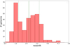 |
Fig. 1. Systemic redshift distribution of galaxies with C III] or He II emission at S/N ≥ 3, selected in this work as described in the text. The green vertical lines represent the median redshift of the sample (continuous line) and the standard deviation of the distribution (dotted lines). |
2.5. Stacking analysis
Even though we can detect and measure ISM velocity shifts for individual galaxies, we also perform spectral stacking to better test the correlations among the different physical parameters. The advantages of stacking are manifold. Firstly, it provides increased statistics as we also include in the stack objects where some ISM absorption lines are undetected. Secondly, we significantly increase the S/N of the stellar continuum, allowing to us check for the presence of faint, broad, or asymmetric wings in the ISM absorption line profiles, which could be indicative of additional outflows or inflows. Furthermore, in the stacking, we can study all the absorption lines in the rest-frame spectral range probed by VANDELS simultaneously, while this is not possible for every individual galaxy, depending on the redshift of each. Finally, we also reduce the uncertainty associated to the ISM shift measurement, and visualise how it is related to the other galaxy properties globally.
The first step of the stacking procedure is the conversion of all our spectra to the rest frame using the systemic redshift estimated in Sect. 2.3 from the C III] or He II emission lines. The spectra are then normalised to the median flux in the range 1570–1601 Å and resampled to a wavelength grid of 1 Å per pixel following the method of our previous works (e.g., Calabrò et al. 2022). Finally, the composite spectra are derived taking the median flux in each pixel wavelength after applying a 3σ clipping to remove outliers. The uncertainty on the stacked spectrum was instead calculated with a bootstrapping resampling procedure as in Calabrò et al. (2022).
We also tested another procedure by taking the weighted average flux in each wavelength pixel to derive the composite spectrum, where the weight is given by the S/N of the emission line (either C III] or He II) that was used for the systemic redshift estimation. This way, spectra with a more accurate estimation of zsys contribute more to the final composite. However, we find that this approach does not lead to significantly different results and therefore we adopt in this paper the first procedure. This should avoid the introduction of subtle systematic biases due to the different contribution of each type of galaxy to the final spectrum, which would be difficult to quantify and control. A representative, high-S/N (≃100) stacked spectrum of all star-forming C III] and He II emitters selected in the previous section is presented in Fig. 2.
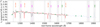 |
Fig. 2. Stack of all star-forming galaxies selected for our analysis (AGNs excluded). The green diamonds represent the pseudocontinuum points used for fitting the cubic spline to the stellar continuum. The red continuous line highlights the combined fit to the Si IIλ1260, Si IIλ1526, C IIλ1334, and Al IIλ1670 absorption lines, while the grey shaded regions have been masked in the fit. The vertical lines highlight the features used in the combined fit (in red), the absorption lines excluded from the combined fit but measured separately (in pink), and the emission lines used for the systemic redshift estimation (in green). |
2.6. Probing the ISM kinematics with absorption lines
After calculating the systemic redshift, we proceed to study the information on the ISM kinematics that can be inferred from the far-UV absorption lines. Here we have more options, that is, a larger number of transitions that we can use to assess the ISM properties. The ISM absorption lines that we detect in individual spectra in the wavelength range from 1000 to 2000 Å are presented in Table 1 and can also be visualised in Fig. 2.
Absorption lines that we detected and fitted in this work, with their rest-frame wavelengths used for the derivation of the ISM velocity shifts.
We note the presence of lower and higher ionisation lines. In the first category reside the Si IIλ1260 and Si IIλ1526 Å absorption lines (dubbed Si IIa and Si IIb in the rest of the paper), C IIλ1334, Al IIλ1670, Fe IIλ1608 Å, and O I Si IIλλ1302-1304 Å (rest-frame vacuum wavelengths). These low-ionisation lines (LIS) mostly trace the neutral and low-ionisation gas in and around galaxies (Shapley et al. 2003). With the exception of O I Si II, all the lines are fitted with the same procedure adopted for the emission lines, that is, with a single Gaussian in absorption plus an underlying continuum modelled with a straight line using windows of 80 Å blueward and redward of the lines.
Given that these windows may overlap with other bright emission or absorption features, when estimating the continuum, we mask the spectral regions corresponding to bright emission lines such as Lyα, N V, C IVλλ1548-1550, O IIIλ1666, C IIIλλ1907-1909, and He IIλ1640, and the broad absorptions due to O I Si IIλλ1302-1304 (when not fitting this line) and C IVλλ1548-1550. This is more important for the spectral stacks and for the Si IIλ1260 and Al IIλ1670 lines. The O I Si II feature is instead modelled as a double Gaussian, fixing the wavelength separation among them. An alternative fitting with a single Gaussian at the median wavelength provides a poorer fit in general, although the results are not significantly affected.
In addition to the LIS, there are also absorption features from higher ionisation species, namely the doublets Si IVλλ1393-1402 and Al IIIλλ1854-1862, where the latter is in general fainter and detected for a lower number of systems, and will therefore be studied systematically only in the composite spectra. In spite of their ISM origin, they also have a stellar wind component which usually manifests as a P-Cygni profile due to the contribution of very young massive stars. The two doublets were fitted with a double Gaussian, fixing the relative wavelength separation and imposing the same velocity width for the two components, but leaving the ratio free to vary between 1 and 1.6, which is the physically allowed range given the electronic densities of local star-forming regions (e.g., Osterbrock & Ferland 2006).
In Fig. 3 we show the distribution of the FWHM for the absorption lines introduced above. In general, Si IIλ1260 and Fe IIλ1608 are the lines detected more frequently in our sample. Besides the fact that they are among the deepest absorption features, the main reason for this is that they lie in a wavelength range covered by VIMOS over almost all of our redshift range, from z = 2 to 5.
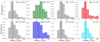 |
Fig. 3. Distribution of FWHM (in km s−1) for the sample selected in this work, for the following absorption lines detected with a S/N ≥ 2: Si IIa, O I Si II, Si IIb, C II, Fe II, Al II, Si IV, and Al III. The vertical lines highlight the median FWHM for each of the lines analysed. |
Overall, the individual observed FWHM values range between 200 and 1800 km s−1, while the medians are all within the range of 550–700 km s−1. The distributions are rather similar, with a 1σ dispersion of 200–300 km s−1 around the median values, depending on the line. In particular, Fe II is the broadest line, with a median FWHM of 680 km s−1. This might be due to a significant absorption component of Fe II at the systemic redshift, and to a contribution from secondary transitions redward of the main Fe II ion line at 1608.45 Å.
At this point we can calculate, for all the ISM lines seen above, the ISM velocity shift (i.e. ISM-shift, or simply vIS), defined as:
 (1)
(1)
where c is the velocity of light, zline is the redshift of each line derived from the best-fit Gaussian centroid, and zsys is the systemic redshift. The uncertainty is derived from the error propagation formula. In Fig. 4 we show the distribution of vIS for each of the absorption lines introduced before. In general, the ISM-shift ranges between −1000 km s−1 and 500 km s−1, meaning that we can have signatures of both gas outflows (negative vIS) and inflows (positive vIS), with a median value that is typically within −200 and +50 km s−1, depending on the line considered.
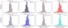 |
Fig. 4. Distribution of ISM shift for the same lines shown in Fig. 3. Symbols and colours are the same as in the previous plot. The two dotted lines in addition to the dashed line of the median represent the standard deviation of vIS values. The number of galaxies contributing to each histogram is written in the top of each panel. |
We checked how the vIS and the FWHM of the lines are related, and we find no correlation between these two quantities. Figure 5 shows an example for the Si IIλ1526 line, which is available for more galaxies in our sample, even though a similar result is also found for the other lines, and for the He II and C III] in emission.
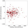 |
Fig. 5. Scatter plot comparing the ISM velocity shift of Si IIλ1526 to the FWHM of the same line (red diamonds). The black squares are the median vIS,Si II calculated in four bins of FWHM. In both cases, it is clear that there is no correlation between the two quantities. A similar result is also obtained for all the other absorption lines. |
In Appendix A.3, we compare vIS inferred from multiple absorption lines (see Figs. A.4–A.5). In particular, we find that the Si IIa, Si IIb, C II, and Al II lines have similar properties in terms of their FWHM and ISM-shift distributions, which are well aligned along the 1:1 correlation with no evident systematic offsets (Fig. A.5). On the other hand, the Fe II line, in addition to having a broader velocity width distribution, shows a positive velocity offset by 100–150 km s−1 compared to the other lines mentioned above, and its median is more consistent with the systemic redshift. However, we caution against the use of the Fe II as a systemic redshift indicator for the parent galaxy population because of the large dispersion in vIS,Fe II for individual galaxies, which also makes the derivation of a systematic correction somewhat uncertain. Although we find a median offset of +40 km s−1 in our sample, we find a significant number of systems with Fe II in outflow or inflow up to ±1000 km s−1 from the central value.
The higher ionisation lines, that is, Al III and Si IV, tend to have lower median velocity shifts compared to the low ionisation lines (by 50 and 110 km s−1, respectively), suggesting larger outflow velocities of the high-ionisation gas, which we discuss further below. Remarkably, we also see that the Al III and Si IV absorption shifts (vIS,Al III and vIS,Si IV) are instead tightly correlated, with no systematic offsets with respect to the 1:1 line. Finally, the O I Si II absorption feature also tends to give higher outflow velocities on average compared to the Si IIλ1526 line by ∼100 km s−1. In this case, the difference might be related to the complex shape and doublet nature of the absorption where the contribution of the two elements in different ionisation states may vary from case to case.
2.7. The combined fit of low-ionisation lines
The results shown in the previous section indicate that the Si IIa, Si IIb, C II, and Al II share similar properties, and therefore in principle they can be fitted together in order to give a unique, combined, and more precise estimate of the low-ionisation and neutral ISM velocity shift. In the combined measurement, we first model the continuum by fitting a cubic spline to the pseudocontinuum ranges identified by Rix et al. (2004) as these relatively free from strong absorption and emission lines, as already done in Calabrò et al. (2021). To these, we add another window blueward of the Si IIλ1260 feature in the rest-frame range 1233.0–1237.0 Å in order to better fit the bluest absorption feature in our spectrum. We then simultaneously fit a single Gaussian to all the individual absorption lines (among the four listed above) that have a S/N of at least 2, fixing the relative distance among them and their velocity width σ. An example of this procedure is shown in Fig. 2 for the whole sample of star-forming galaxies with a good estimate of zsys. We derived vIS,comb using all four lines in 50 galaxies, using three lines in 127 galaxies, using two lines in 67 galaxies, and using one low-ionisation line with S/N≥ 2 in 55 galaxies. The output FWHM and ISM velocity shift from the combined fit agree overall with the typical values found when using the individual features separately and when using the average or the median of the lines available.
To further check which lines should be considered in the combined fit, we also run a combined measurement including all possible far-UV absorption lines in the fit (both those in pink and in red in Fig. 2), and then calculating the number of outliers for which the combined ISM velocity shift differs from the individual line estimation by more than 200 km s−1. The result of this exercise is shown in Fig. A.3. Imposing an outlier threshold of 10%, O I Si II, Si IV, Fe II, and Al III are automatically excluded, while the remaining lines (Si IIa, Si IIb, C II, and Al II) have outlier fractions of less than 5%, confirming their similar nature. Throughout this paper we therefore use and refer to the combined fit as a single, simultaneous fit to all the available low-ionisation lines among the four listed above.
While for the spectral stacking we use the whole sample of 330 star-forming galaxies selected as C III] or He II emitters with a good estimation of the systemic redshift, the ISM absorption lines (and therefore a measurement of the ISM velocity shift) are available for a smaller number of objects than the original one. In particular, we have a combined fit measurement of the low-ionisation absorption lines (vIS,comb) for 299 galaxies, while the Si IV line (and therefore an estimate of vIS,Si IV) is available for 166 objects. We use these two measurements in the results section to study the low-ionisation and high-ionisation gas kinematics, respectively, as a function of other physical properties of our sample. The exact number of galaxies for which a particular ISM absorption line is detected with S/N ≥ 2 is instead indicated above each histogram in Fig. 4. We also note that choosing a higher S/N threshold for the inclusion of a low-ionisation absorption line in the combined fit does not change the results. Moreover, we should keep in mind that the combination of multiple features fitted at the same redshift significantly reduces the possibility of spurious detections, meaning that we can be confident of the presence of the absorption lines even if we decrease the S/N requirement on the single feature to 2.
2.8. The maximum ISM velocity
While the bulk velocity describes the global kinematic properties of the ISM, in reality the gas component in a galaxy shows a range of velocities, which can translate into narrower or broader absorption line widths. In order to understand the final fate of the gas, it is also useful to constrain the maximum velocity at which the gas is flowing outwards, indicated as vmax.
This quantity can be derived following the methodology of Zakamska & Greene (2014). In the most general, non-parametric approach, it is based on the cumulative velocity distribution as  , where f(v) is the best-fit spectrum modelled around the absorption feature and translated into velocity space. We then define vmax as the velocity (always reported to the systemic redshift) at which 2% of the total flux of the line accumulates, which analytically is the solution to the equation F(v) = 0.02, if F(v) is normalised to the total flux. This also corresponds to v02 which is typically used in the literature.
In this work, the lines are well described as single Gaussians, in which case vmax is simply related to the line FWHM and can be calculated as
![Mathematical equation: $$ \begin{aligned} { v}_{\rm max} [\mathrm{km\,s}^{-1}] = 0.872 \times FWHM_{\rm line} + { v}_{\rm ISM,line} , \end{aligned} $$](/articles/aa/full_html/2022/11/aa44364-22/aa44364-22-eq5.gif) (2)
(2)
where vISM, line is the velocity shift of the line centroid itself with respect to zsys, and FWHMline is the intrinsic line width deconvolved from the instrumental broadening. Furthermore, given the spectral resolution of VANDELS, the absorption lines are marginally resolved, and therefore we need a high S/N to accurately measure the intrinsic FWHM. For this reason, we only apply this analysis to the spectral stacks in Sect. 3.2.
2.9. Galaxies with positive ISM velocity shift
An important piece of evidence from the histograms presented in Fig. 4 is that a small but significant number of sources, depending on the specific line considered, shows a positive ISM velocity shift, which is indicative of a global inflow. This result is confirmed with the analysis of the combined fit, suggesting that positive velocities are not due to noise or found only for specific lines in the galaxies, but rather that all the low-ionisation lines have consistent kinematics. In particular, we find that 34% of our sample has vIS,comb ≥ 0. We analyse the physical properties of this subset (e.g., M⋆, SFR, and morphology) below, and also compare to the global population.
To check the robustness of this result, we selected only galaxies for which the low-ionisation absorption lines that contribute to the combined fit have a S/N > 3 instead of 2. This way, we find that the fraction of objects that still have vIS,comb ≥ 0 is 32%. Even by increasing the detection threshold of the C III] line used for systemic redshift estimation to 5, we still get a fraction of 35%. For explicative purposes, Fig. 6 shows two examples at redshifts ∼2.5 and 3.5 of galaxies where we detect positive low-ionisation ISM velocities of significantly above zero.
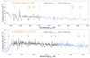 |
Fig. 6. Figure shows the spectrum of two galaxies at redshifts 2.587 and 3.479 in the UDS and CDFS field (top and bottom panels, respectively) with the combined fit of low-ionisation absorption lines (red), and for which we detect significant inflow signatures, with positive ISM velocity shifts as indicated in each panel (i.e. the centroids of ISM absorption lines are redshifted compared to the C III] centroid used for the systemic redshift). |
2.10. Fitting the SiIV doublet
A single component Gaussian yields a good fit to the absorption line profiles for most of the galaxies in our sample. However, we notice that in some cases, the Si IV feature, which has among the largest absorption equivalent widths and is therefore easier to detect even in galaxies with a modest S/N continuum, shows a residual absorption in the bluer part. This suggests that an additional blueshifted component should be added in the fit.
In order to identify these cases, we systematically fitted all the spectra in the Si IV range with a double component, which – as this line is already a doublet – translates into four Gaussians in absorption fitted simultaneously. In this fit, we imposed that the two Si IV Gaussians of the extra component have the same velocity width, as in the two main Si IV absorptions. Moreover, we set a maximum FWHM for the new component to three times the FWHM of the main one, and a maximum velocity difference between the two of 2000 km s−1 in order to avoid unrealistically broad absorption features. Finally, we compared the reduced χ2 ( ) values obtained through a single component fit with those given by the new procedure. We then selected the galaxies where the additional outflow component flux has a S/N of at least 3, and, following Zakamska & Greene (2014), where the double component fit decreases the
  by ≥5% compared to the previous approach. We obtain a total of 22 galaxies satisfying all the above requirements and showing evidence of asymmetric profiles of Si IV. The main Gaussian component, which might be already shifted with respect to the systemic redshift, is closer to the lower ionisation line velocity shift, while the second is more blueshifted by on average 1000 km s−1. We also notice that such an additional Gaussian component is always fainter than the main Si IV absorption, with a typical flux ratio of 0.05.
The Si IV doublet has in general a complex shape because, in addition to the ISM absorption, it can include P-cygni-like, metallicity-dependent, stellar wind features produced by O-type stars (Castor et al. 1975; Kaper et al. 1992). This P-cygni profile, with a strongly blueshifted absorption component, becomes stronger at older ages or at higher stellar metallicities (Drew 1989; Pauldrach et al. 1990). For this reason, the entire Si IV observed profile, including the fainter blueshifted absorption wing, is difficult to interpret. It may be an additional outflow component, representing gaseous clouds with a higher bulk velocity compared to the main, deeper absorption measured from a single Gaussian fit. Alternatively, it can be related to stellar physics.
In order to search for the correct hypothesis, we compare the observed Si IV absorption feature with multiple stellar models, including Starburst99 (S99, Leitherer et al. 2010), BPASS with binary stars (Eldridge et al. 2017; Stanway & Eldridge 2018; Xiao et al. 2018), and Beagle (Chevallard & Charlot 2016), which is based on the latest version of Bruzual & Charlot (2003) stellar population models. For this exercise, we take the spectral stack of all star-forming galaxies selected in this work in order to have the highest possible S/N around the Si IV feature and detect even the finest stellar features.
The spectral comparison is shown in Fig. 7, where the best-fit model is chosen using a χ2 minimisation approach and always corresponds to the closest stellar metallicity Z⋆ derived for star-forming galaxies at similar redshifts in previous VANDELS works (see Calabrò et al. 2021). The models also have a stellar age of ≃100 Myr. We can see that S99 and BC03 models, while nicely reproducing the shape of the stellar continuum on the two sides of the Si IV feature, are mostly flat on top of the ISM absorption feature and do not reproduce the additional Si IV component. On the other hand, the BPASS model considered in the last panel (with a metallicity log (Z⋆/Z⊙) = − 0.85) can almost perfectly reproduce the extra blueshifted absorption component of Si IV, which is displaced by exactly the same amount (namely ∼1000 km s−1) as the observed difference between the main Si IV absorption peak and the best-fit centroid of the extra component.
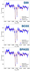 |
Fig. 7. Spectral region around the ISM+stellar Si IV absorption doublet. In all the panels, the blue line is the stacked spectrum of all star-forming galaxies with C III] or He II emission selected in this work, where the error bars at each pixel represent the 1σ error. The orange line is the best-fit Gaussian made with MPFIT, assuming two Gaussian components for each side of the doublet (i.e. four Gaussians in total), as explained in the text. The red lines represent the best-fit models from Starburst99 (S99), Beagle (i.e. BC03 models), and BPASS, from top to bottom, respectively. The best-fit models have the closest stellar metallicity Z⋆ to the median of our galaxies (Calabrò et al. 2021), that is, log (Z⋆/Z⊙) = − 0.7 for S99, −0.82 for BC03, and −0.85 for BPASS. We reiterate the fact that the measured Z⋆ using BPASS calibrations is 0.1 dex lower than S99. |
Furthermore, we find that the additional blueshifted Si IV absorption is preferentially found in galaxies with higher stellar masses and SFRs, but is also detected when stacking together galaxies at lower M⋆ and SFR, or all those that do not show this extra component individually. This result indicates that we are dealing with an intrinsic physical property of the Si IV line arising from stellar winds of more evolved O-type stars, and predicted only by the BPASS models. The reason for this might be related to a combination of the inclusion of binary stars and the different modelling of the stellar evolution. The detection of this feature for only a small subset of galaxies might also be related to the different stellar ages of individual systems, where more evolved galaxies might have a stronger Si IV P-Cygni feature, according to BPASS models. However, it can be easily detected when stacking together multiple systems, because we are both increasing the S/N of the continuum and averaging among a wide range of stellar ages.
In the following part of the paper, we refer to the Si IV line as the component originating in the interstellar medium only. Therefore, in the spectral stacks that we show in Sects. 3.1–3.2, and for the 22 galaxies mentioned above where the extra blueshifted component was significantly detected, we always perform a four-Gaussian fit to decontaminate the absorption profile from the contribution of the stellar wind, and measure peak wavelength, total flux, and FWHM only for the ISM component. Given the low equivalent width of this additional feature and the displacement of ∼1000 km s−1 of its peak, it does not significantly affect the properties of the main Si IV absorption when the extra-component is not detected.
We also checked in the above subset for the simultaneous presence of blueward asymmetric profiles in other lower ionisation absorption lines. While for the Al II feature it is difficult to make this test due to the nearby emission of the O IIIλ1666 line and Al III has on average a much lower S/N in individual galaxies, we do not find evidence of bluer or redder additional components in the Si IIa, Si IIb, or C II lines for our galaxies. This again suggests that the blue wing of the Si IV feature does not represent an additional outflow component, which we would otherwise detect also in the other lines, at least in the stacks.
2.11. Galaxy physical properties from SED fitting
For the entire sample of galaxies selected in the previous section, we infer their fundamental physical properties, including stellar mass (M⋆) and star-formation rate (SFR), from multi-wavelength photometric catalogues available in the VANDELS fields. In the central parts of CDFS and UDS, which is covered by CANDELS (Grogin et al. 2011; Koekemoer et al. 2011), the photometry is taken from Guo et al. (2013) and Galametz et al. (2013), respectively, which reach HAB ∼ 25.5 and ∼26.7 magnitudes at ∼90% completeness. For the extended region outside CANDELS, our collaboration produced new photometric catalogues from ground-based optical and near-infrared observations, reaching a depth of HAB = 24.5 and 25 magnitudes in the CDFS and UDS fields, respectively.
After assembling the whole catalogue, we use the Beagle software (BayEsian Analysis of GaLaxy sEds) developed by Chevallard & Charlot (2016) to fit in a Bayesian fashion the stellar population models of Gutkin et al. (2016) to the observed photometry from U-band to IRAC channel 2, fixing the redshift to the systemic value derived in Sect. 2.3. We adopt an exponentially delayed star-formation history (SFH ∼ τexp−τ, where τ is the typical star-formation time), a Chabrier IMF, and we calculate the current SFR value over the last 100 Myr. The value of log τ was initialised with a uniform prior ranging 7.0–10.5 (in yr), while the specific SFR (SSFR) and the maximum stellar age were allowed to assume any value in the range −9.5 < log(SSFR) < − 7.05 (in yr−1) and 7 < log(age) < 10.2 (in yr). Similarly, the stellar mass M⋆ and the stellar metallicity Z⋆ were also assigned, respectively, a uniform prior in the range 5 < log(M⋆/M⊙) < 12 and a Gaussian prior centred at log(Z⋆/Z⊙) = − 0.85 (1σ = 0.2), following previous results based on the VANDELS survey from Cullen et al. (2019) and Calabrò et al. (2021). The dust attenuation of the galaxy, modelled with a Charlot & Fall (2000) law, is described through the V-band optical attenuation depth τV, and initialised with a uniform prior in the range of 0–10 mag. The Inoue et al. (2014) model is used instead for the attenuation of the intergalactic medium (IGM). In our Beagle run, in addition to photometric data, we also fit the observed C IIIλλ1907-1909, He IIλ1640, and C IVλλ1548-1550 emission line fluxes (which are the brightest emission features in the far-UV), setting a 2σ upper limit in case of non-detections. These lines are used by the code to constrain the ionisation parameter (initialised with a uniform prior in the range −4 < log(U) < − 1) using the grid of photoionisation models by Gutkin et al. (2016). This way, Beagle also better takes into account nebular contamination to the photometric bands. Finally, we set the dust-to-metal ratio ξd and the ratio between interstellar medium depth and total optical depth μ = τISM/τV to 0.3, which are typical values for star-forming galaxies according to Camps et al. (2016) and Battisti et al. (2020).
Plotting together the SFR and stellar mass M⋆ obtained from Beagle, we see that our subset of 330 galaxies is representative of the star-forming main sequence at the redshift of this work (Fig. 8) in the stellar mass range from 108 to 1010 M⊙, where our median relation is just slightly offset upwards compared to that derived by Speagle et al. (2014), but still within their 1σ scatter of 0.2 dex, which is also the average uncertainty of our SFR measurements. For M⋆ > 1010, we probe slightly higher specific SFRs, placing galaxies ∼ + 0.3 dex above the MS at z = 3. In this high-mass regime, we also find a small subset of ten galaxies in the starburst regime with SFR at least four times higher than the MS, following the definition by Rodighiero et al. (2011). As shown by Llerena et al. (2022), C III] emitters are fairly representative of the entire star-forming galaxy population observed with VANDELS (including also non emitters), sharing a similar distribution of mass and SFR. The bias towards higher SFRs at M⋆ > 1010 M⊙ is indeed related to the original VANDELS selection, picking up slightly brighter and more star-forming galaxies in that mass range. However, we checked that the results of this paper do not change significantly, even when considering the population of galaxies with M⋆ < 1010 M⊙.
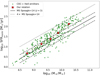 |
Fig. 8. Star-formation rate–stellar mass diagram for the sample of 330 C III] + He II emitters selected for our analysis. The main sequence relation by Speagle et al. (2014) is drawn with a black continuous line, while the dashed parallel lines represent the 1σ dispersion and the dotted line the starburst limit (4× above the main sequence). Our best-fit M⋆–SFR relation is represented with large red stars. On the y axis, we consider the SFR normalised to z = 3 assuming the evolving trend with redshift as (1 + z)2.8 from Sargent et al. (2012). |
2.12. Morphological analysis
2.12.1. Merger identification
Gas inflows or outflows can be produced by galaxy interactions, which can funnel significant fractions of gas towards the centre of the gravitational potential well, usually corresponding to a starburst core (Di Matteo et al. 2005; Calabrò et al. 2019) or eject gas into the outskirts as a consequence of tidal forces and feedback (Rupke et al. 2005; Di Matteo et al. 2007). It is therefore important to carry out a qualitative assessment of the morphology of galaxies, identifying those systems that are undergoing an interaction and where the merger phenomenon can play a role in the gas kinematics.
A subset of 226 galaxies from our original sample of C III] + He II emitters have high-resolution HST-ACS F814W images available (probing around 2000 Å rest-frame at our redshifts), which allows us to perform a statistical morphological analysis and to identify merging systems, with the best resolution and depth achievable with current capabilities. This subset covers not only the CANDELS regions in CDFS and UDS, but is distributed over a wider area, including the wider CDFS field targeted by VANDELS, which in recent years has been covered with HST in the same band i. As a result, almost all of the originally selected galaxies lying in CDFS and half of those falling in UDS can be used for our morphological analysis. We assigned a merger class to them (0= non-merger, and 1= merger) as we explain in the following.
Given the relatively small size of our sample of C III] emitters, we decided to identify mergers from visual inspection, which allows us to check interactively and more carefully for the presence of double nuclei and interacting signatures. A visual classification has already been applied to the CANDELS fields by Kartaltepe et al. (2015, hereafter K15) for 50 000 galaxies spanning the redshift range 0 < z < 4, with classifications from three to five independent people for each object. For their merger sample (i.e. our merger class = 1), these authors considered sources with double nuclei or with evidence of bright tidal features such as tails, loops, bridges, and very disturbed morphologies, all of which are suggestive of an ongoing major interaction. The interaction can be within the same segmentation map, or rather with a companion galaxy that can be still clearly distinguishable. All these cases fall in the interaction classes 1, 2, or 3 in K15. We note that disturbed morphologies in the UV rest-frame can also be due to the presence of bright stellar clumps in a more regular galaxy.
We adopt the K15 classification for galaxies in the CANDELS regions, while we use the same procedure to classify in i-band the remaining galaxies that fall in the CDFS wide area targeted by VANDELS. In our redshift range, we expect to have an intense growth of galaxies through gas accretion or merging events with smaller companions or satellites, resulting in large gas fractions, unstable discs, and very asymmetric and clumpy morphologies. For this reason, a very conservative approach is adopted in the classification, not including in the merger sample those galaxies with only minor morphological disturbances, such as faint asymmetric features, small companions, or off-centre clumps.
We find a total of 64 mergers, which represent a fraction of ∼30% of the sample with HST images available. The first row of Fig. 9 shows three examples of merger systems within our C III] + He II line emitters, with different characteristic interacting features. The bottom row also shows the comparison with a subset of different types of isolated, non-interacting galaxies, including both discy and more spheroidal systems. The second of these images explains our conservative procedure: despite the faint asymmetric emission leftward of the main disc, we do not include that galaxy in the merger sample as there is no clear evidence of a major, ongoing interaction.
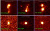 |
Fig. 9. HST F814W images (Koekemoer et al. 2011) of three galaxies with reliable systemic redshift and ISM-shift estimations. Upper row: these galaxies are visually identified as merging or interacting systems, as showing, from left to right, bridges connecting the interacting components, a very disturbed and asymmetric morphology, and a double nucleus. Bottom row: three examples of isolated or non-interacting galaxies with a discy shape (first case) and a more spheroidal structure (second and third image). |
2.12.2. Size measurement and concentration parameter
In low-redshift observations and simulations, ISM outflows induced by star-formation feedback have been shown to be ubiquitous in galaxies above some SFR surface density (ΣSFR) threshold, typically ΣSFR > 0.1 M⊙ yr−1 kpc−2 (e.g., Heckman et al. 2011; Sharma et al. 2017). Several studies also found a correlation of this quantity with the outflow velocity (e.g., Heckman et al. 2015). It is therefore worth checking for possible correlations between the ISM kinematic properties and ΣSFR in our work. This parameter, in addition to the SFR, requires measurement of the physical sizes of the star-forming regions in the system. Given that our SFRs are UV-based, we also measure the sizes from optical (observed) HST images, which probe the UV rest frame of the galaxies.
Because of the large fraction of irregular, asymmetric, and clumpy galaxies at redshifts ≥2 (Guo et al. 2012; Huertas-Company et al. 2016), whose structures do not yet resemble the regular shapes of the Hubble sequence seen at lower redshift, a parametric fitting (e.g., with a Sersic profile) tends to severely underestimate the size (Law et al. 2007; Ribeiro et al. 2016, hereafter R16). Therefore, despite the fact that Sersic parameters are publicly available for the CANDELS data, as provided by Griffith et al. (2012) and van der Wel et al. (2014), although these catalogues do not cover the wider CDFS field targeted by VANDELS, we decided to follow a non-parametric approach by adopting the equivalent radius as a size measurement, using exactly the same procedure defined in R16 and already applied successfully in the VUDS survey at similar redshifts. The equivalent radius  (in kpc) is defined analytically as:
![Mathematical equation: $$ \begin{aligned} r_{T}^{x}\ [\mathrm{kpc}] = \sqrt{\frac{T_{x}}{\pi } }. \end{aligned} $$](/articles/aa/full_html/2022/11/aa44364-22/aa44364-22-eq9.gif) (3)
(3)
The variable Tx (in kpc2) in the above equation is given by:
![Mathematical equation: $$ \begin{aligned} T_x\ [\mathrm{kpc}^2]= N_x L^2 \left( 2\times 10^{-11} \frac{{\mathrm{ster} }}{{\mathrm{arcsec} ^{2}}}\right) D_{A}^{2}, \end{aligned} $$](/articles/aa/full_html/2022/11/aa44364-22/aa44364-22-eq10.gif) (4)
(4)
where Nx is the number of pixels (with size L in arcsec/pixel) that sum up to x% of the total flux of the galaxy, while DA is the angular diameter distance. The quantity  is also corrected for PSF broadening effects following Eq. (18) of R16.
The advantages of this definition are that we do not need to assume a surface brightness profile, and therefore it does not depend on the galaxy shape, on the aperture definitions, on initial guesses, or on the convergence of a fit. Even though it can be calculated in principle with any percentage x comprised between 0% and 100%, we consider in our work  , which counts the brightest pixels summing up to 50% of the galaxy flux, and is more similar to the effective radius from GALFIT that is often adopted.
Another useful morphological parameter describing the light profile of the galaxy is the concentration, which was modified from the original definition of Bershady et al. (2000) to take into account the asymmetric and irregular structure of high-redshift galaxies. The new concentration parameter CT is calculated (following R16) from the two equivalent radii  and
and  as
as
 (5)
(5)
Compared to the standard definition of concentration, the advantage of this new quantity is that it does not depend on the definition of a galaxy centre, and it is not affected by the presence of multiple bright clumps or irregular morphologies and therefore works more efficiently in characterising the light profiles in the case of typical galaxies found in the early Universe. As shown by R16, the usual definition tends to underestimate the true light concentration in the case of asymmetric profiles or highly inhomogeneous emission. More details on the derivation of  and CT can be found in R16.
In Fig. 10, we show the histogram distribution of  and CT for our sample of C III] and He II emitters with available HST F814W images and morphological parameters. Our galaxies have
  ranging from 0.3 to 2.7 kpc, with the mergers identified in the previous section having amongst the highest spatial extensions, because for these systems
  includes the size of two merging systems rather than one. On the other hand, the light concentration CT ranges between 2 and 3.75, with a median value of 2.5, which is consistent with the typical values found by R16 (their Fig. 18) for star-forming galaxies from z = 2 to z = 4. As discussed in R16, we also find that
  correlates well with the Sersic radius for a subset of CANDELS galaxies where re was estimated in previous works.
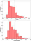 |
Fig. 10. Histogram distribution of the equivalent radius |

3. Results
In this section, we show how the bulk ISM velocity shift vIS and the maximum velocity vmax are related to other fundamental galaxy properties that we derived in Sect. 2. Our aim here is to understand the physical origin of the broad range of vIS and vmax values spanned by our galaxies. We perform the analysis on vIS both for individual galaxies, where we can check for peculiar ISM velocities, and on a global perspective, using the composite spectra of objects with similar properties. In order to explore the relation globally, we bin the sample in multiple groups, adopting the first, second, and third interquartile values as bin separations, which usually ensures an adequate S/N to our purposes for the stacked spectrum in each bin.
3.1. Dependence of the bulk ISM velocity on galaxy properties
Following the previous findings, we first test the relations of vIS with the stellar mass and SFR. In particular, we analyse the velocity shift vIS,comb from the combined fit of low-ionisation lines (i.e. Si IIa, Si IIb, C II, and Al II), and that derived from higher ionisation lines as vIS,Si IV. Al III behaves similarly to Si IV but is available for fewer individual objects because it is a fainter absorption, and therefore we consider it later in the stacking analysis.
The results for vIS,comb and vIS,Si IV are shown in Fig. 11 for each of the above two physical parameters. In all four diagrams, we do not find any significant correlations between M⋆ (or SFR) and vIS for individual galaxies. Considering all the sources, we indeed obtain very low Pearson correlation coefficients (ρ < 0.1 in absolute value) with high p-values, indicating that our findings are consistent with no dependence between these quantities in the parameter space spanned by our galaxies. We also divide our sample in four subsets using the interquartile ranges of the stellar mass and SFR, calculating the median M⋆ and SFR of all the galaxies residing in the same bin, and then estimating vIS,comb and vIS,Si IV from the stacks. This way, we obtain a median relation representative of the whole population, drawn with black empty squares in Fig. 11, which also suggests that the trend is not significantly different from constant for both low-ionisation absorption lines and for Si IV. As confirmation of this result, the angular coefficient of the best-fit lines to all the individual points in the diagrams is always consistent with zero. We can also better appreciate the larger dispersion of Si IV velocities compared to the lower ionisation lines, as we have seen in Fig. 4, and in particular the higher number of sources with ISM velocities < − 500 km s−1, that is, higher outflow velocity. Interestingly, the presence of outliers or peculiar systems, with inflow (outflow) velocities above (below) the median velocity by more than 1σ, does not correlate with either M⋆ or SFR in any of the cases. These extreme cases therefore do not seem to have different properties compared to the average population.
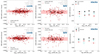 |
Fig. 11. Upper panel: correlation of vIS,comb, vIS,Si IV and vIS,Al III with the stellar mass M⋆ for VANDELS star-forming galaxies selected in this work. The first two panels in each row show the relation for individual galaxies (red diamonds), while the black empty squares are the median vIS in bins of increasing M⋆. The red horizontal continuous line shows the median vIS for the entire sample shown in each plot, while the red shaded regions highlight the standard deviation of all the ISM shift values. The last panel of the row shows the velocity shifts calculated directly from the spectral stacks in four bins of stellar mass. Lower panel: same as above but as a function of the SFR. |
In the last column of Fig. 11, we show the results obtained in a different way by measuring the ISM-velocity shifts directly from the spectral stacks instead of individual galaxies. In this case, we also add the measurements for the Al IIIλλ1854-1862 doublet, which is better detected in the stacked spectra. Using the same previous bins of M⋆ and SFR, we can understand from this exercise that also from a global perspective there are no significant variations as a function of these two quantities for vIS,comb, vIS,Si IV, and vIS,Al III.
We then analysed the dependence of the ISM velocity shift on morphology-related parameters, namely the physical size as  , the concentration CT, and the SFR surface density ΣSFR. The results are shown in Fig. 12 for both individual galaxies and for the spectral stacks, after defining bins of increasing
  , CT, and ΣSFR. As before, we focus on the velocity shifts of the LIS (through the combined fit) and of higher ionisation lines including Al III and Si IV.
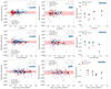 |
Fig. 12. Diagrams comparing vIS,comb, vIS,Si IV and vIS,Al III to the equivalent radius |

In the first row, where physical size is represented, we find a weak and marginally significant correlation between  and vIS, as indicated by the low Pearson correlation coefficient (and p-value < 0.05) from both the combined fit of LIS lines. We should note that the median vIS is slightly lower (i.e. higher outflow velocity) for galaxies of smaller sizes, and this is also true when considering the Si IV line. In the stacking analysis in the last panel, vIS,comb of galaxies with
  kpc is below the median population value at the 1σ level, and its difference compared to smaller galaxies is significant at 2σ. A similar difference is also found for Al III and Si IV between galaxies with
  lower and higher than ∼1.5 kpc.
For the concentration parameter displayed in the second row of Fig. 12, we can see that a correlation, although weak, exists with vIS,comb and vIS,Si IV already for individual galaxies, as indicated by the results of the Pearson correlation test. Moreover, we can see in the third panel that the stack of galaxies with a higher concentration parameter (CT > 3) has vIS,comb, vIS,Si IV, and vIS,Al III that are lower by ∼50, 100, and 150 km s−1, respectively, compared to galaxies with less concentrated UV emission and CT ≤ 3, with a significance of 2σ on average. However, we also notice that the lower vIS,comb and vIS,Si IV at high concentration parameter is mostly driven by non-merger systems (Fig. 12). This difference is similar to the downward offset that we observe in the median vIS of the Si IV line for galaxies residing in the last bin of CT (second panel of the second row).
Finally, we show the relation with ΣSFR in the last row of Fig. 12. Given the weak correlation with  , with this new parameter we also find a similarly weak dependence on vIS. Indeed, the Pearson correlation coefficient and the linear best-fit slope indicate a significance of 2σ when considering the low-ionisation lines for individual galaxies. For Si IV, even though the correlation is not significant, we notice that the highest outflow velocities (i.e. lowest vIS,Si IV) also tend to have higher ΣSFR in the stacked analysis.
Overall, there are no significant correlations between the bulk ISM velocity (in all the ionisation states that we probed) on stellar mass and SFR, while a weak trend (marginally significant at 2σ) is found for the other three parameters, indicating that galaxies with more concentrated emission (CT ≳ 3), smaller size, and higher ΣSFR might launch faster outflows.
As already shown in Fig. 4, in all the right panels of Figs. 11–12, we then notice on average a systematic difference in vIS among the various types of far-UV absorption lines that we detect in VANDELS spectra. The combined fit, which traces the kinematics of the low-ionisation lines, indicates that the neutral ISM in a typical star-forming galaxy is outflowing, with average |vIS,comb| of 60 ± 10 km s−1. On the other hand, higher ionisation lines such as Si IV and Al III trace gas that is moving away from galactic centres at higher velocities of 170 ± 30 km s−1 and 160 ± 30 km s−1, respectively. In Fig. 13, we can see the different velocity profiles (normalised to the range +700–1000 km s−1) of the absorption lines in the stacked spectrum constructed from the full sample of 330 star-forming galaxies with C III] or He II emission and therefore with a systemic redshift measurement. The Gaussian centroid of Si IIλ1526, which we take as representative of low-ionisation lines tracing neutral gas, is shifted towards negative velocities (−100 km s−1) compared to the systemic redshift. Fe IIλ1608 has a broader profile, is less deep, and is centred at slightly positive ISM shifts close to the systemic redshift. On the other hand, Si IVλλ1393-1402 and Al IIIλλ1854-1862 have blueshifted Gaussian centroids, with larger vIS in outflow by 100 km s−1 compared to the low-ionisation line Si IIb. We further discuss the velocity difference between these two gas phases in Sect. 4.3. In Table 2, we summarise the correlation strengths between vIS and all the galaxy properties studied in this work.
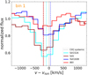 |
Fig. 13. Comparison of the line profiles in the spectral stack including all star-forming galaxies selected in this work (AGNs excluded). The central wavelengths resulting from a Gaussian fit are highlighted in cyan, blue, red, and dark red for the Si IIλ1526 line (representative of low-ionisation lines), Fe IIλ1608, Al IIIλλ1854-1862, and Si IVλλ1393-1402, respectively. |
Pearson correlation coefficients ρ (with corresponding p-values) between the ISM velocity shifts of low-ionisation lines and Si IV, and different physical properties of the galaxies that we analyse in this paper.
3.2. Dependence of the maximum ISM velocity on galaxy properties
We now explore the dependence of the maximum velocity for the same galaxy parameters seen in the previous section. Compared to the bulk ISM velocity, vmax carries more information about the gas flows as it also depends on the absorption line width. As mentioned in Sect. 2.8, we performed the analysis on the spectral stacks, and we consider only the combined fit of low-ionisation lines and Si IV for which we have a higher S/N.
In order to test the dependence with the same physical properties analysed in the previous section, we divided our sample into four groups of similar properties (using the interquartile ranges), and then stacked the spectra and calculated vmax in each bin. The diagrams for all the parameters are shown in Fig. 14. Here we can see that globally, we find similar results to the previous analysis based on the bulk ISM velocity. In particular, we find a similar decreasing trend of vmax for smaller galaxies and highly concentrated systems (significance > 3σ), although the second case is valid only from the combined fit where we have a higher S/N. Compared to the previous section, we find here a marginally significant (∼2σ) relation between vmax and both the SFR and ΣSFR, for both the lower and higher ionisation lines. In the latter diagram, the weak trend is mainly driven by the last bin, where galaxies with ΣSFR > 1 M⊙ yr−1 kpc−2 show maximum outflow velocities that are approximately 300 km s−1 higher than the remaining population at lower ΣSFR. Finally, for the stellar mass we also find more negative vmax at M⋆ > 1010 M⊙, but only from the Si IV line analysis. Overall, we find that vmax is on average better correlated with the galaxy physical properties compared to vIS, although the correlations remain weak and marginally significant, and, similarly, slightly more important for morphological related quantities.
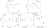 |
Fig. 14. Diagrams comparing vmax,comb and vmax,Si IV (estimated from stacked spectra) to other physical properties of the galaxies, namely the stellar mass M⋆, the SFR, the equivalent radius |

3.3. Outflows in mergers and redshift evolution
Finally, we also tested the effects of mergers on gas kinematics in high-redshift star-forming galaxies. According to Chisholm et al. (2015), mergers at z ∼ 0 can drive faster outflows than isolated galaxies. In our case, we can see already in Figs. 11–12 for individual galaxies that visually identified mergers (cyan diamonds) are distributed over the whole range of explored parameters and have a similar distribution in M⋆, SFR, ΣSFR, and concentration to that of more isolated galaxies. In the first row of Fig. 12, we note that mergers tend to have larger sizes  , which is reasonable considering that they are often composed of two or more interacting components, each with its own size.
Furthermore, we have performed a stack of all identified merger systems in the selected sample, in order to better compare with the rest of the population of non-merger galaxies. The results are shown in the top panel of Fig. 15, in which we can see that mergers and non-merger galaxies (respectively indicated with a merger label 1 or 0) have similar ISM kinematics. Indeed, we find that the bulk velocities are consistent within the uncertainties at the 1–2σ level for all the lines, both the higher ionisation (as vIS,Si IV and vIS,Al III) and lower ionisation lines (vIS,comb).
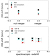 |
Fig. 15. Dependence of the ISM velocity shift vIS on the merger flag (1 = mergers and 0 = non-mergers) and spectroscopic redshift. Each symbol represents a spectral stack in a different redshift or merger flag bin. The colours highlight the results from the combined fit of low-ionisation lines (black squares), Si IV (red circles), and the Al III absorption line (cyan triangles). |
Finally, considering the wide range of redshifts (from 2 to 5) probed by VANDELS, as represented in Fig. 1, we also checked for a possible evolution in redshift of the outflow properties in star-forming galaxies, measuring vIS,comb, vIS,Si IV and vIS,Al III in spectral stacks in bins of increasing redshift. The results of this exercise are shown in the bottom panel of Fig. 15, and again indicate that there is no difference in the average outflow velocity as a function of redshift for the low and higher ionisation lines, as no significant correlation is found. Despite the slightly higher outflow velocity from Si IV at z ∼ 2.7, this is still consistent with the other bins within 1σ.
4. Discussion
We show in the above sections that, considering the galaxy population as a whole, the interstellar medium traced by UV absorption lines is on average moving with a velocity of −60 km s−1 along the line of sight (hence globally in outflow) for the low-ionisation gas, which rises up to ∼ − 170 km s−1 for higher ionisation gas. This is confirmed both by averaging the ISM velocities of individual galaxies and by performing spectral stacks in bins of different physical parameters. Furthermore, we measure maximum velocities of the gas in the outflow direction ranging between 500 and 800 km s−1 for most of our sample. In the following, we compare our results to studies of the ISM kinematics at lower redshift, and then move to a more physical investigation of the effects of outflows on galaxy evolution.
4.1. Comparison with works at lower redshifts
Galactic outflows at different cosmic epochs have been studied for decades. In the local Universe, Heckman et al. (2015) studied star-formation-driven winds from far-UV absorption lines (Si IIa,Si IIb, C II, and Si IV) in a sample of 39 galaxies spanning a broad range of stellar masses and SFRs, detecting bulk ISM velocities from 100 to 200 km s−1, globally in outflow. Interestingly, they report strong correlations between ISM bulk velocities and both SFR and ΣSFR.
At intermediate redshifts, ISM kinematic properties have been characterised in large samples of star-forming galaxies. Bordoloi et al. (2014) analysed 486 galaxies at 1 ≤ z ≤ 1.5, with log(M⋆/M⊙) and log(SFR/M⊙ yr−1) ranging from 9.45 to 10.7 and 0.14 to 2.35, respectively, finding typical ISM velocities vIS of ∼150–200 km s−1 from the MgII absorption doublet. Furthermore, vIS was found to correlate with ΣSFR but not with the SFR itself. Furthermore, Weiner et al. (2009) used the same MgII absorption to calculate vIS for a sample of ∼1400 galaxies at z ∼ 1.4 with similarly massive galaxies of the previously mentioned work, and a broad range of SFRs from 10 to 100 M⊙ yr. These authors found slightly higher typical outflow velocities of ∼300 to 500 km s−1, increasing both as a function of stellar mass and SFR, in analogy to local infrared-luminous galaxies.
If we move to earlier cosmic epochs, Talia et al. (2012) studied ISM flows, with the same methodology as that used here, in 74 star-forming galaxies in the stellar mass range from 109.2 to 1010.6 M⊙ at redshifts of 1.4 to 2.8 (zmedian ∼ 2), finding a median ISM velocity of 100 km s−1 and no significant dependence of vIS on galaxy properties. Similarly, Steidel et al. (2010) derived vIS from the position of C II, Si IV, Si IIa, and Si IIb far-UV absorption lines for a statistical sample of 89 Lyman-break galaxies at 2 < z < 2.6 (zmedian = 2.3) and slightly more massive (M⋆ > 109.5 M⊙). While these later authors found a slightly higher ISM velocity than us (=164 ± 16 km s−1), they report no correlations of vIS with the main galaxy properties including M⋆ and SFR. Our results therefore extend this lack of correlation up to at least z ∼ 4.5.
Interestingly, we find on average ISM velocities closer to zero compared to previous works. Moreover, as noted in Sect. 2.9, we find that 34% of our galaxy sample has a positive velocity shift, indicative of a global inflow. This fraction is approximately double that found by Steidel et al. (2010), and we reach higher inflow velocities on average for the low- and high-ionisation absorption lines. Overall, our findings suggest that, for the same levels of SFR and stellar mass of the host galaxies, the bulk of the ISM moves closer to systemic from low redshift to high redshift, and becomes less sensitive to variations of the star formation activity and mass budget. This might be due to an increased role of inflows at earlier cosmic times, which might prevail over star-formation-driven outflows in the majority of systems. Regarding these inflows, while we know from theory that cosmological metal-poor gas condensation and accretion onto galaxies should occur at early epochs (z ≳ 2), it is difficult from our data and measured velocities to disentangle gas accretion from the cosmic web from that originating in galactic fountains. A key test would be the measurement of the gas-phase metallicity of the outflowing and inflowing gas, which would require a higher spectral resolution and sensitivity, and will be addressed in a future work.
We remark that we are exploring an epoch where the bulk of the galaxy population is rapidly assembling through mergers and gas inflows, and they have a more gas-rich and turbulent ISM. Combining gas infall episodes and these additional effects to stellar-driven feedback might produce multiple absorption components with different relative velocities and with different absorption strengths, of which we measure only a median, spatially integrated, line-of-sight-dependent value for each galaxy. In other words, we might have as a net result the weakening of outflow signatures compared to lower redshift star-forming galaxies, even though part of the gas can still be moving outwards with high velocity in some galaxies, with some material reaching high speeds of up to vIS ∼ 1000 km s−1.
At the same time, the weak trends and lack of correlation of vIS with the main galaxy properties can be explained by the same arguments. However, additional effects might be at play. For example, Bordoloi et al. (2014) find that face-on galaxies at intermediate redshift (1–1.5) have higher velocity outflows as compared to edge-on galaxies at similar redshifts and stellar masses, while Roberts-Borsani et al. (2020) find that outflows are most powerful in the central regions of massive star-forming galaxies, even though this was studied in the local Universe. In order to check these additional dependences, we need to observe statistical samples with IFU instruments and better spatial resolution in order to disentangle the different components of the ISM in high-redshift galaxies. We also note that, because of the slightly biased selection (towards higher SFRs) at high stellar masses (M⋆ > 1010 M⊙), the trend is less representative of the global star-forming population in that regime, and completely unconstrained at even higher masses than those probed by VANDELS (i.e. M⋆ ≳ 1011 M⊙). Future spectroscopic surveys probing larger volumes could help to better constrain this parameter space.
4.2. Outflow physical properties and mass loading factor
In this section, we focus on the physical properties and driving mechanisms of outflows in the average star-forming population at z ∼ 3.5. Therefore, in the following part of the paper, we consider only VANDELS galaxies for which we measure a global outflow, that is, a negative bulk ISM velocity vIS,comb (or vIS,Si IV). If we restrict the sample to these objects, we obtain average outflow velocities of −146 ± 10 km s−1 for the former and −270 ± 30 km s−1 for the latter, which are more similar to the typical ISM velocities measured at intermediate redshifts in the works described in the previous section. We remark that even if we consider only this reduced sample, there would be no significant changes in the correlation results presented in Sects. 3.1 and 3.2 between the bulk outflow velocity (or vmax) and the other galaxy physical properties. Taking these results on the outflow velocities, we are now ready to quantitatively assess the effects of star-formation-driven winds on the host galaxies by computing the mass-outflow rate, mass-loading factor, and typical escape velocities of our systems.
We calculate the mass-outflow rate Ṁout in a thin shell approximation as
 (6)
(6)
where CΩ and Cf are the angular and clumpiness covering fraction, respectively, μmp is the mean atomic weight, R is the radius of the thin shell wind, and vISM is the gas outflow velocity, assumed to be the typical bulk ISM velocity measured from our spectra. As we are deriving an average value over many galaxies viewed from different angles, and because in the stacking procedure we are integrating over lines of sight and clumpiness with different covering fractions, we fix CΩCf = 1, as in Bordoloi et al. (2014). We also set μ = 1.4, and we infer the outflow radius R as the average equivalent radius estimated for our sample in Sect. 2.12.2, which is ∼1 kpc. Finally, NH is the column density of the outflowing gas, which can be estimated as in Leitherer et al. (2011) and Heckman et al. (2011) from the dust attenuation properties of our galaxies (assuming a Calzetti law), taking into account also a secondary dependence with the metallicity, as
 (7)
(7)
Taking the median E(B − V) = 0.194 mag measured for our sample from the available photometric data as described in Calabrò et al. (2021), and considering the typical gas-phase metallicity of 0.4 × Z⊙ derived for VANDELS galaxies at z ∼ 3 (Cullen et al. 2021), we infer NH = 1.75 × 1021 cm−2. Using all these values in Eq. (6), we get
![Mathematical equation: $$ \begin{aligned} {\dot{M}_{\rm out} [M_\odot \,\mathrm{yr}^{-1}] \;\simeq 36\ \frac{N_H}{10^{21.24}\, \mathrm{cm}^{-2}} \times \frac{R}{1\, \mathrm{kpc}} \times \frac{{ v}_{\rm ISM}}{146\, \mathrm{km\,s}^{-1}}} .\end{aligned} $$](/articles/aa/full_html/2022/11/aa44364-22/aa44364-22-eq34.gif) (8)
(8)
The mass outflow rate estimated in this way is comparable to the SFR of the galaxies, and yields an outflow mass loading factor η of the order of unity, or just slightly above. In particular, considering the median SFR of our sample of 196 galaxies with a net outflow signature (SFRmedian = 27 M⊙ yr−1), we derive:
 (9)
(9)
which is nicely consistent with the values found with a similar methodology for low-ionisation gas outflows in local and intermediate redshift (z ∼ 1–1.5) star-forming galaxies (Heckman et al. 2015; Bordoloi et al. 2014). We also note that a similar η was found for ionised and cold molecular outflows in purely star-forming galaxies at z < 0.2 (Fluetsch et al. 2019), once we homogenise the assumptions on the wind geometry adopted in the two papers. However, these later authors probe 1.5 dex higher stellar masses than our study.
With the above information, we can study the nature of the outflows. From a physical perspective, when stellar winds impact the surrounding ISM, a shock front is created, which injects energy into the gaseous medium and then propagates outwards, sweeping the gas away from the galactic centre. The outflows can be classified into two types, depending on the efficiency of the radiative cooling during the shock propagation. In momentum-driven flows, the total momentum is conserved, while most of the preshock kinetic energy is radiatively lost, which produces a rapid cooling of baryons in a thin shell of gas and a strong discontinuity with the post-shock region. On the other hand, in energy-driven flows, the shock expands adiabatically into the ISM preserving most of its mechanical luminosity, and therefore cooling is negligible, and the flow is much more violent compared to the previous mechanism. In order to identify the nature of the outflow and distinguish between the two driving mechanisms, we can compare the energy and momentum rate of the outflow to the momentum and luminosity input from star formation. The outflow-related properties are written, respectively, as ṗout = Ṁout vISM and  . The momentum and energy from star formation are instead given by ṗrad = LSFR/c and Ėrad = LSFR, where LSFR/L⊙ ∼ 1010× SFR/M⊙ yr−1 (Kennicutt 1998). Assuming the median SFR of our sample with a net outflow (vISM < 0), this yields
 (10)
(10)
which indicates that we are witnessing momentum-driven winds.
Finally, we study the fate of the outflows in VANDELS galaxies by comparing the observed outflow velocities to those needed to escape from the gravitational potential wells of the galaxies. The escape velocity is related, using dynamical arguments, to the circular velocity vc as vesc ≃ 3 × vc for reasonable halo mass distributions (Binney & Tremaine 1987; Heckman et al. 2000). The circular velocity instead can be estimated observationally from the emission line width σvel along the line of sight using the relation σvel ∼ 0.6 × vc, where σvel represents an average over all the observed inclinations (Fig. 7 of Rix et al. 1997). Putting this information together, we obtain the relation vesc ≃ 5 × σvel. We remark that this is a median relation that is subject to large uncertainties depending on the geometry and internal dynamics of the galaxies; however it gives a useful indication, and can be compared with our ISM velocities.
In the far-UV spectral range covered by VANDELS, the brightest emission lines are C III] and He II. While the former is a doublet and difficult to model given the resolution of VANDELS, the latter has in general a lower S/N and a larger scatter, with a skewed distribution towards broader profiles compared to C III]. For these reasons, we instead used the optical rest-frame O II line, which was also used for the calculation of vesc in the previously mentioned works. In our case, this line was covered by the follow-up of a subset of galaxies with MOSFIRE, which has a resolving power reaching ≃3650 in band H (Cullen et al. 2021).
Considering the values of 11 individual galaxies where the O II line was detected with a minimum S/N of 5, and which have a similar mass distribution to our subset, we obtain an average σ[OII] of 125 km s−1. Using this estimate as representative of our sample to calculate the escape fraction, we get vesc of the order of 625 km s−1. This is well above the average bulk outflow velocities that we measure in our galaxies from both lower and higher ionisation lines. It is also higher compared to the estimates of vIS,comb and vIS,Si IV for the majority of individual galaxies. However, it is intereresting to note that a small fraction of objects, where the bulk outflow velocity is amongst the highest in our sample, might be the best candidates to launch significant amounts of gas outside of the systems.
Considering the stacking analysis performed in Sect. 3.2, we note that even the average maximum velocity vmax, as defined in Sect. 2.10, does not generally overcome vesc. This implies that, for the average population and for a broad variety of conditions, most of the ISM is expected to remain bound to the main galaxy halo, even though we might exceed this limit when we consider galaxies with the highest stellar masses, SFRs, ΣSFR, and concentration (i.e. smaller size) among those probed in this work. Therefore, there is a greater probability that gas will escape from galaxies with more extreme properties.
4.3. Low- versus high-ionisation gas outflows
We find that the ISM-shift of Si IV and Al III indicates a faster velocity of the higher ionisation outflowing gas by approximately 100 km s−1 compared to vIS,comb of low-ionisation lines (i.e. Si II, C II, Al II) derived from the combined fit. To understand the physical origin of this difference of bulk outflow velocities (and also vmax), we need to better investigate the properties of our absorption lines.
A first approach is based on looking at the ionisation potential required for the creation of a particular species. The Si IV and Al III species require an ionisation potential of 45 eV and 28 eV, respectively, which is higher than low-ionisation lines, which need ionisation energies of 16, 19, and 24 eV for the Si II, Al II, and C II ions, respectively. It is clear that, by their nature, low-ionisation elements require denser, self-shielded gas to survive while the high-ionisation elements can survive in more rarefied, less dense regions. Secondly, we can use different transitions of the same ionisation species to probe the optical depth of the absorbing gas. In the case of high-ionisation lines, they come already in close doublets, while for the low-ionisation gas, we can use the two transitions of the Si II ion. The individual components of the high-ionisation doublets have similar oscillator strengths f1 and f2 of ∼0.5 and 0.25 for the bluer and redder component, respectively, indicating that in both cases we should expect an equivalent width ratio of EW1/EW2 = ( )/(
)/( ) = 0.5 in the optically thin case (see also Erb et al. 2012). For the Si IV doublet, we observe an EW ratio of
  , while for Al III we obtain a similar value of
  . In an optically thick absorbing gas, the ratio no longer depends on the oscillator strength and approaches a value of 1. The results imply that we are in an intermediate condition, even though we are actually closer to the optically thin limit. For the two transitions of the Si II ion, at ≃1260 Å and 1526 Å, their different oscillator strengths (f1 = 1.22 and f2 = 0.13) imply an expected ratio in the optically thin case of 0.156. We measure an observed ratio of
  , where the larger uncertainties derive from the fact that the two lines are not close in wavelength and do not share the same continuum level as in the high-ionisation doublets. Despite the large uncertainty, this calculation indicates that the EW ratio is consistent with the optically thick case.
Both approaches therefore suggest that low-ionisation lines probe denser gas. To understand the physical implications of this, we can look at galactic wind models. If we take for simplicity the spherical, momentum driven wind model of Murray et al. (2005), the gas density is predicted to rapidly decline with radius (∼r−2 − r−3), which is also reasonable considering that the wind is subject to geometrical dilution at larger distances from the galactic centre. The same model predicts that the wind is accelerating as an effect of radiation pressure pushing onto dust grains, with velocity increasing towards larger radii. We notice that accelerating winds seem to also be more consistent with observations of local starburst galaxies (Martin & Bouché 2009) and high-redshift Lyman-break galaxies, as discussed in Steidel et al. (2010). They also better reproduce the resolved profile of the MgII absorption line in star-forming galaxies at z ∼ 1.4 (Weiner et al. 2009). It is therefore clear that, according to this simple model, highly ionised gas, which traces more rarefied gas regions far from the centre, should also move faster, which is exactly what we observe in our sample of star-forming galaxies at z > 2. We stress again that this model is a simplistic assumption and is by no means the best or the only model describing star-formation-driven winds. However, despite all the assumptions made, we must recognise that it provides an easy framework with which to interpret our observations.
In conclusion, the most plausible physical explanation of the velocity difference observed between low- and high-ionisation lines relies on the fact that they come from slightly different spatial regions of the galaxies, at different distances from the centre. Therefore, they likely trace gas in different conditions of density and temperature, with low-ionisation gas probing the denser and colder star-forming cores, while higher ionised material is more widespread, optically thin, and likely coming from the outer shell of the expanding winds.
5. Summary and conclusions
In this paper, we present our study of the ISM kinematics of 330 star-forming galaxies with a systemic redshift estimated through C III] or He II detection with S/N ≥ 3 in the redshift range between 2 and 4.5 (zmedian ≃ 3.1), and in the stellar mass range from 108 to 1011 M⊙. We derived the kinematic properties from a large variety of ISM absorption lines, which are compared to the systemic redshift inferred from C III] or He II, and then related to different physical properties of the host galaxies. We summarise the main findings of this paper as follows.
-
The ISM in typical star-forming galaxies at redshifts 2–5 (zmedian ≃ 3) and with stellar masses of between 108 and 1011 M⊙ is globally in outflow, with a median bulk velocity vIS of ∼ − 60 ± 10 km s−1 for low-ionisation gas traced by Si IIλ1260, C IIλ1334, Si IIλ1526, and Al IIλ1670, and 200 > vIS > 150 km s−1 for higher ionisation gas traced by Si IV and Al III. Individual galaxies can have ISM velocities spanning the range ±1000 km s−1, with higher ionisation gas reaching higher velocities on average and with a larger dispersion around the median value.
-
Our sample includes a fraction of galaxies (34%) with positive velocity shift obtained from the combined fit of low-ionisation lines, indicating the prevalence of inflowing material in those systems. This fraction is approximately double that found in similar works at lower redshift (e.g., Steidel et al. 2010), suggesting a more important role of inflows at earlier epochs in the Universe.
-
We do not find significant correlations between the bulk ISM velocity shift (vIS, vIS,comb, vIS,Si IV, vIS,Al III) and the stellar mass M⋆ or SFR of the galaxies, while a marginally significant (i.e. at 2σ level) correlation is found with the size (probed by the equivalent radius
 ), light concentration parameter CT, and SFR surface density ΣSFR.
 -
In spectral stacks, we also measure the maximum velocity vmax, defined as the velocity at which 2% of the absorption line flux accumulates. We find that vmax in our sample has on average a value of ∼ − 500 and ∼ − 600 km s−1 for the low-ionisation and high-ionisation gas (traced by Si IV), respectively.
-
Compared to the bulk velocity, vmax is more closely related to galaxy properties. Galaxies with a higher stellar mass, SFR, concentration, ΣSFR, and more compact size launch outflows with higher maximum velocities on average, even though the correlations remain weak, with a significance of ≃2σ for SFR-related quantities (i.e. SFR and ΣSFR), and slightly higher significance for the morphology-related parameters.
-
We detect a complex shape of the Si IV absorption feature, which shows a main absorption component arising in the ISM and closer to the systemic redshift, and a fainter, additional absorption component likely originating in stellar winds, which is blueshifted from the main absorption peak by ∼1000 km s−1. We find that BPASS models with binary populations, at odds with the BC03 and S99 models, are able to perfectly reproduce the blueshifted stellar wind absorption component of the line. This complex shape can be detected in both spectral stacks and some individual galaxies with higher S/N.
-
Mergers show similar or slightly lower outflow velocities compared to non-merging systems, suggesting that inflows and internal turbulence induced by the interaction might dilute the outflow signatures coming from star-formation feedback.
-
Considering the 196 galaxies with a net outflow velocity (i.e. a negative vIS,comb), we obtain average outflow velocities of −146 ± 10 km s−1 for the low-ionisation gas and −270 ± 30 km s−1 for the high ionisation component traced by Si IV. From them we calculate, in a spherically symmetric thin shell approximation, the mass outflow rate Ṁout of the gas, which is comparable to the star formation of the galaxies (η ≃ 1.3). The values of Ṁout and vIS are also in favour of radiation-pressure-driven outflows.
-
We derive a rough estimate of the escape velocity expected in our galaxies of vesc = 625 km s−1. This is higher than the average bulk and also maximum outflow velocity derived for our sample, even though for a small fraction of galaxies we can have ∣vIS,comb∣ and ∣vIS,Si IV∣ > vesc.
In the near future, spatially resolved studies with IFU instruments, such as NIRSpec with JWST and ERIS at the VLT, will provide better insight into the different components of the ISM in high-redshift galaxies, and into the possible local relationships between kinematics and physical properties. Their higher spectral resolution will also allow the intrinsic profile of absorption lines to be characterised, even for individual galaxies. Similarly, ALMA can provide spatially resolved maps on the cold molecular gas, which would help to better assess the nature and final fate of the outflows, constraining their role on galaxy evolution.
Acknowledgments
We thank the anonymous referee for constructive comments. A.C. acknowledges the support from grant PRIN MIUR 2017 20173ML3WW_s. R.A. acknowledges support from ANID Fondecyt Regular 1202007. Based on observations collected at the European Southern Observatory under ESO programme(s) 194.A-2003.
References
- Asplund, M., Grevesse, N., Sauval, A. J., et al. 2009, ARA&A, 47, 481 [Google Scholar]
- Battisti, A. J., Cunha, E. D., Shivaei, I., et al. 2020, ApJ, 888, 108 [NASA ADS] [CrossRef] [Google Scholar]
- Behroozi, P. S., Wechsler, R. H., & Conroy, C. 2013, ApJ, 770, 57 [NASA ADS] [CrossRef] [Google Scholar]
- Bershady, M. A., Jangren, A., & Conselice, C. J. 2000, AJ, 119, 2645 [NASA ADS] [CrossRef] [Google Scholar]
- Binney, J., & Tremaine, S. 1987, Galactic Dynamics (Princeton: Princeton Univ. Press) [Google Scholar]
- Bordoloi, R., Lilly, S. J., Hardmeier, E., et al. 2014, ApJ, 794, 130 [NASA ADS] [CrossRef] [Google Scholar]
- Bothwell, M. S., Maiolino, R., Kennicutt, R., et al. 2013, MNRAS, 433, 1425 [Google Scholar]
- Bouché, N., Dekel, A., Genzel, R., et al. 2010, ApJ, 718, 1001 [Google Scholar]
- Bouché, N., Finley, H., Schroetter, I., et al. 2016, ApJ, 820, 121 [Google Scholar]
- Brooks, A. M., Governato, F., Quinn, T., et al. 2009, ApJ, 694, 396 [NASA ADS] [CrossRef] [Google Scholar]
- Bruzual, G., & Charlot, S. 2003, MNRAS, 344, 1000 [NASA ADS] [CrossRef] [Google Scholar]
- Calabrò, A., Amorín, R., Fontana, A., et al. 2017, A&A, 601, A95 [NASA ADS] [CrossRef] [EDP Sciences] [Google Scholar]
- Calabrò, A., Daddi, E., Cassata, P., et al. 2018, ApJ, 862, L22 [Google Scholar]
- Calabrò, A., Daddi, E., Puglisi, A., et al. 2019, A&A, 623, A64 [NASA ADS] [CrossRef] [EDP Sciences] [Google Scholar]
- Calabrò, A., Castellano, M., Pentericci, L., et al. 2021, A&A, 646, A39 [EDP Sciences] [Google Scholar]
- Calabrò, A., Guaita, L., Pentericci, L., et al. 2022, A&A, 664, A75 [NASA ADS] [CrossRef] [EDP Sciences] [Google Scholar]
- Camps, P., Trayford, J. W., Baes, M., et al. 2016, MNRAS, 462, 1057 [CrossRef] [Google Scholar]
- Cantalupo, S., Arrigoni-Battaia, F., Prochaska, J. X., et al. 2014, Nature, 506, 63 [NASA ADS] [CrossRef] [Google Scholar]
- Castor, J. I., Abbott, D. C., & Klein, R. I. 1975, ApJ, 195, 157 [Google Scholar]
- Cattaneo, A., Faber, S. M., Binney, J., et al. 2009, Nature, 460, 213 [NASA ADS] [CrossRef] [Google Scholar]
- Cazzoli, S., Arribas, S., Maiolino, R., et al. 2016, A&A, 590, A125 [NASA ADS] [CrossRef] [EDP Sciences] [Google Scholar]
- Chabrier, G. 2003, PASP, 115, 763 [Google Scholar]
- Charlot, S., & Fall, S. M. 2000, ApJ, 539, 718 [Google Scholar]
- Chevalier, R. A. 1977, ARA&A, 15, 175 [NASA ADS] [CrossRef] [Google Scholar]
- Chevalier, R. A., & Clegg, A. W. 1985, Nature, 317, 44 [Google Scholar]
- Chevallard, J., & Charlot, S. 2016, MNRAS, 462, 1415 [NASA ADS] [CrossRef] [Google Scholar]
- Chisholm, J., Tremonti, C. A., Leitherer, C., et al. 2015, ApJ, 811, 149 [NASA ADS] [CrossRef] [Google Scholar]
- Chisholm, J., Tremonti, C. A., Leitherer, C., et al. 2017, MNRAS, 469, 4831 [NASA ADS] [CrossRef] [Google Scholar]
- Combes, F., García-Burillo, S., Braine, J., et al. 2013, A&A, 550, A41 [NASA ADS] [CrossRef] [EDP Sciences] [Google Scholar]
- Concas, A., Maiolino, R., Curti, M., et al. 2022, MNRAS, 513, 2535 [NASA ADS] [CrossRef] [Google Scholar]
- Croton, D. J., Springel, V., White, S. D. M., et al. 2006, MNRAS, 365, 11 [Google Scholar]
- Cullen, F., McLure, R. J., Dunlop, J. S., et al. 2019, MNRAS, 487, 2038 [Google Scholar]
- Cullen, F., Shapley, A. E., McLure, R. J., et al. 2021, MNRAS, 505, 903 [CrossRef] [Google Scholar]
- Daddi, E., Valentino, F., Rich, R. M., et al. 2021, A&A, 649, A78 [NASA ADS] [CrossRef] [EDP Sciences] [Google Scholar]
- Davé, R., Finlator, K., & Oppenheimer, B. D. 2011, MNRAS, 416, 1354 [CrossRef] [Google Scholar]
- Davé, R., Finlator, K., & Oppenheimer, B. D. 2012, MNRAS, 421, 98 [Google Scholar]
- Dayal, P., & Ferrara, A. 2018, Phys. Rep., 780, 1 [Google Scholar]
- De Lucia, G., Springel, V., White, S. D. M., et al. 2006, MNRAS, 366, 499 [NASA ADS] [CrossRef] [Google Scholar]
- Dekel, A., & Birnboim, Y. 2006, MNRAS, 368, 2 [NASA ADS] [CrossRef] [Google Scholar]
- Dekel, A., Birnboim, Y., Engel, G., et al. 2009, Nature, 457, 451 [Google Scholar]
- Dekel, A., Zolotov, A., Tweed, D., et al. 2013, MNRAS, 435, 999 [Google Scholar]
- Di Matteo, T., Springel, V., & Hernquist, L. 2005, Nature, 433, 604 [NASA ADS] [CrossRef] [Google Scholar]
- Di Matteo, P., Combes, F., Melchior, A.-L., et al. 2007, A&A, 468, 61 [NASA ADS] [CrossRef] [EDP Sciences] [Google Scholar]
- Drew, J. E. 1989, ApJS, 71, 267 [NASA ADS] [CrossRef] [Google Scholar]
- Eldridge, J. J., Stanway, E. R., Xiao, L., et al. 2017, PASA, 34, e058 [Google Scholar]
- Erb, D. K., Quider, A. M., Henry, A. L., et al. 2012, ApJ, 759, 26 [CrossRef] [Google Scholar]
- Fabian, A. C. 2012, ARA&A, 50, 455 [Google Scholar]
- Feltre, A., Charlot, S., & Gutkin, J. 2016, MNRAS, 456, 3354 [Google Scholar]
- Fluetsch, A., Maiolino, R., Carniani, S., et al. 2019, MNRAS, 483, 4586 [NASA ADS] [Google Scholar]
- Fontanot, F., Hirschmann, M., & De Lucia, G. 2017, ApJ, 842, L14 [Google Scholar]
- Fontanot, F., Calabrò, A., Talia, M., et al. 2021, MNRAS, 504, 4481 [CrossRef] [Google Scholar]
- Förster Schreiber, N. M., Übler, H., Davies, R. L., et al. 2019, ApJ, 875, 21 [Google Scholar]
- Fraternali, F. 2017, Gas Accretion Galaxies, 430, 323 [NASA ADS] [CrossRef] [Google Scholar]
- Galametz, A., Grazian, A., Fontana, A., et al. 2013, ApJS, 206, 10 [Google Scholar]
- Garilli, B., Fumana, M., Franzetti, P., et al. 2010, PASP, 122, 827 [Google Scholar]
- Garilli, B., McLure, R., Pentericci, L., et al. 2021, A&A, 647, A150 [NASA ADS] [CrossRef] [EDP Sciences] [Google Scholar]
- Griffith, R. L., Cooper, M. C., Newman, J. A., et al. 2012, ApJS, 200, 9 [NASA ADS] [CrossRef] [Google Scholar]
- Grogin, N. A., Kocevski, D. D., Faber, S. M., et al. 2011, ApJS, 197, 35 [NASA ADS] [CrossRef] [Google Scholar]
- Guo, Y., Giavalisco, M., Ferguson, H. C., et al. 2012, ApJ, 757, 120 [NASA ADS] [CrossRef] [Google Scholar]
- Guo, Y., Ferguson, H. C., Giavalisco, M., et al. 2013, ApJS, 207, 24 [NASA ADS] [CrossRef] [Google Scholar]
- Gutkin, J., Charlot, S., & Bruzual, G. 2016, MNRAS, 462, 1757 [Google Scholar]
- Harrison, C. M. 2017, Nat. Astron., 1, 0165 [NASA ADS] [CrossRef] [Google Scholar]
- Harrison, C. M., Alexander, D. M., Swinbank, A. M., et al. 2012, MNRAS, 426, 1073 [NASA ADS] [CrossRef] [Google Scholar]
- Heckman, T. M., & Borthakur, S. 2016, ApJ, 822, 9 [CrossRef] [Google Scholar]
- Heckman, T. M., Lehnert, M. D., Strickland, D. K., et al. 2000, ApJS, 129, 493 [NASA ADS] [CrossRef] [Google Scholar]
- Heckman, T. M., Borthakur, S., Overzier, R., et al. 2011, ApJ, 730, 5 [Google Scholar]
- Heckman, T. M., Alexandroff, R. M., Borthakur, S., et al. 2015, ApJ, 809, 147 [NASA ADS] [CrossRef] [Google Scholar]
- Hennawi, J. F., Prochaska, J. X., Cantalupo, S., et al. 2015, Science, 348, 779 [NASA ADS] [CrossRef] [Google Scholar]
- Hopkins, P. F., Kereš, D., Oñorbe, J., et al. 2014, MNRAS, 445, 581 [NASA ADS] [CrossRef] [Google Scholar]
- Huertas-Company, M., Bernardi, M., Pérez-González, P. G., et al. 2016, MNRAS, 462, 4495 [CrossRef] [Google Scholar]
- Inoue, A. K., Shimizu, I., Iwata, I., et al. 2014, MNRAS, 442, 1805 [Google Scholar]
- Kaper, L., Henrichs, H. F., & Nichols-Bohlin, J. 1992, in ASP Conf. Ser., 30, 135 [NASA ADS] [Google Scholar]
- Kartaltepe, J. S., Mozena, M., Kocevski, D., et al. 2015, ApJS, 221, 11 [NASA ADS] [CrossRef] [Google Scholar]
- Katz, N., Keres, D., Dave, R., et al. 2003, The IGM/Galaxy Connection. The Distribution of Baryons at z=0, eds. J. L. Rosenberg, M. E. Putman (Dordrecht: Kluwer Academic Publishers), 281, 185 [CrossRef] [Google Scholar]
- Kennicutt, R. C. 1998, ApJ, 498, 541 [NASA ADS] [CrossRef] [Google Scholar]
- Kereš, D., Katz, N., Weinberg, D. H., et al. 2005, MNRAS, 363, 2 [CrossRef] [Google Scholar]
- Kocevski, D. D., Hasinger, G., Brightman, M., et al. 2018, ApJS, 236, 48 [CrossRef] [Google Scholar]
- Koekemoer, A. M., Faber, S. M., Ferguson, H. C., et al. 2011, ApJS, 197, 36 [NASA ADS] [CrossRef] [Google Scholar]
- Kormendy, J., & Ho, L. C. 2013, ARA&A, 51, 511 [Google Scholar]
- L’Huillier, B., Combes, F., & Semelin, B. 2012, A&A, 544, A68 [NASA ADS] [CrossRef] [EDP Sciences] [Google Scholar]
- Law, D. R., Steidel, C. C., Erb, D. K., et al. 2007, ApJ, 656, 1 [NASA ADS] [CrossRef] [Google Scholar]
- Leitherer, C., Ortiz Otálvaro, P. A., Bresolin, F., et al. 2010, ApJS, 189, 309 [Google Scholar]
- Leitherer, C., Tremonti, C. A., Heckman, T. M., et al. 2011, AJ, 141, 37 [Google Scholar]
- Lilly, S. J., Carollo, C. M., Pipino, A., et al. 2013, ApJ, 772, 119 [NASA ADS] [CrossRef] [Google Scholar]
- Llerena, M., Amorín, R., Cullen, F., et al. 2022, A&A, 659, A16 [NASA ADS] [CrossRef] [EDP Sciences] [Google Scholar]
- Luo, B., Brandt, W. N., Xue, Y. Q., et al. 2017, ApJS, 228, 2 [Google Scholar]
- Madau, P., Ferguson, H. C., Dickinson, M. E., et al. 1996, MNRAS, 283, 1388 [Google Scholar]
- Mannucci, F., Cresci, G., Maiolino, R., et al. 2009, MNRAS, 398, 1915 [Google Scholar]
- Marasco, A., Fraternali, F., & Binney, J. J. 2012, MNRAS, 419, 1107 [NASA ADS] [CrossRef] [Google Scholar]
- Marchi, F., Pentericci, L., Guaita, L., et al. 2019, A&A, 631, A19 [NASA ADS] [CrossRef] [EDP Sciences] [Google Scholar]
- Markwardt, C. B. 2009, in Astronomical Data Analysis Software and Systems XVIII, eds. D. A. Bohlender, D. Durand, & P. Dowler, (San Francisco: Astronomical Society of the Pacific) 411, 251 [Google Scholar]
- Martin, C. L., & Bouché, N. 2009, ApJ, 703, 1394 [NASA ADS] [CrossRef] [Google Scholar]
- McLure, R. J., Pentericci, L., Cimatti, A., et al. 2018, MNRAS, 479, 25 [NASA ADS] [Google Scholar]
- Miller, N. A., Bonzini, M., Fomalont, E. B., et al. 2013, ApJS, 205, 13 [NASA ADS] [CrossRef] [Google Scholar]
- Murray, N., Quataert, E., & Thompson, T. A. 2005, ApJ, 618, 569 [NASA ADS] [CrossRef] [Google Scholar]
- Nakajima, K., Schaerer, D., Le Fèvre, O., et al. 2018, A&A, 612, A94 [NASA ADS] [CrossRef] [EDP Sciences] [Google Scholar]
- Ocvirk, P., Pichon, C., & Teyssier, R. 2008, MNRAS, 390, 1326 [Google Scholar]
- Osterbrock, D. E., & Ferland, G. J. 2006, in Astrophysics of Gaseous Nebulae and Active Galactic Nuclei, eds. D. E. Osterbrock, & G. J. Ferland, (Sausalito, CA: University Science Books), 2nd edn. [Google Scholar]
- Pauldrach, A. W. A., Kudritzki, R. P., Puls, J., et al. 1990, A&A, 228, 125 [NASA ADS] [Google Scholar]
- Pentericci, L., McLure, R. J., Garilli, B., et al. 2018, A&A, 616, A174 [NASA ADS] [CrossRef] [EDP Sciences] [Google Scholar]
- Pettini, M., Rix, S. A., Steidel, C. C., et al. 2002, ApJ, 569, 742 [NASA ADS] [CrossRef] [Google Scholar]
- Ribeiro, B., Le Fèvre, O., Tasca, L. A. M., et al. 2016, A&A, 593, A22 [NASA ADS] [CrossRef] [EDP Sciences] [Google Scholar]
- Rix, H.-W., Guhathakurta, P., Colless, M., et al. 1997, MNRAS, 285, 779 [NASA ADS] [CrossRef] [Google Scholar]
- Rix, S. A., Pettini, M., Leitherer, C., et al. 2004, ApJ, 615, 98 [Google Scholar]
- Roberts-Borsani, G. W., Saintonge, A., Masters, K. L., et al. 2020, MNRAS, 493, 3081 [NASA ADS] [CrossRef] [Google Scholar]
- Rodighiero, G., Daddi, E., Baronchelli, I., et al. 2011, ApJ, 739, L40 [Google Scholar]
- Rodríguez-Puebla, A., Primack, J. R., Behroozi, P., et al. 2016, MNRAS, 455, 2592 [CrossRef] [Google Scholar]
- Rubin, K. H. R., Prochaska, J. X., Koo, D. C., et al. 2014, ApJ, 794, 156 [Google Scholar]
- Rupke, D. S., Veilleux, S., & Sanders, D. B. 2005, ApJS, 160, 115 [Google Scholar]
- Sargent, M. T., Béthermin, M., Daddi, E., et al. 2012, ApJ, 747, L31 [NASA ADS] [CrossRef] [Google Scholar]
- Saxena, A., Pentericci, L., Mirabelli, M., et al. 2020, A&A, 636, A47 [NASA ADS] [CrossRef] [EDP Sciences] [Google Scholar]
- Schaye, J., Dalla Vecchia, C., Booth, C. M., et al. 2010, MNRAS, 402, 1536 [Google Scholar]
- Shapley, A. E., Steidel, C. C., Pettini, M., et al. 2003, ApJ, 588, 65 [Google Scholar]
- Sharma, M., Theuns, T., Frenk, C., et al. 2017, MNRAS, 468, 2176 [NASA ADS] [CrossRef] [Google Scholar]
- Shirazi, M., & Brinchmann, J. 2012, MNRAS, 421, 1043 [NASA ADS] [CrossRef] [Google Scholar]
- Silk, J., & Mamon, G. A. 2012, Res. Astron. Astrophys., 12, 917 [Google Scholar]
- Simpson, C., Martínez-Sansigre, A., Rawlings, S., et al. 2006, MNRAS, 372, 741 [NASA ADS] [CrossRef] [Google Scholar]
- Speagle, J. S., Steinhardt, C. L., Capak, P. L., et al. 2014, ApJS, 214, 15 [NASA ADS] [CrossRef] [Google Scholar]
- Stanway, E. R., & Eldridge, J. J. 2018, MNRAS, 479, 75 [NASA ADS] [CrossRef] [Google Scholar]
- Steidel, C. C., Erb, D. K., Shapley, A. E., et al. 2010, ApJ, 717, 289 [Google Scholar]
- Tacchella, S., Dekel, A., Carollo, C. M., et al. 2016, MNRAS, 457, 2790 [Google Scholar]
- Talia, M., Mignoli, M., Cimatti, A., et al. 2012, A&A, 539, A61 [NASA ADS] [CrossRef] [EDP Sciences] [Google Scholar]
- van der Wel, A., Franx, M., van Dokkum, P. G., et al. 2014, ApJ, 788, 28 [Google Scholar]
- Veilleux, S., Cecil, G., & Bland-Hawthorn, J. 2005, ARA&A, 43, 769 [NASA ADS] [CrossRef] [Google Scholar]
- Veilleux, S., Maiolino, R., Bolatto, A. D., et al. 2020, A&ARv, 28, 2 [NASA ADS] [CrossRef] [Google Scholar]
- Weiner, B. J., Coil, A. L., Prochaska, J. X., et al. 2009, ApJ, 692, 187 [Google Scholar]
- Xiao, L., Stanway, E. R., & Eldridge, J. J. 2018, MNRAS, 477, 904 [Google Scholar]
- Zabl, J., Bouché, N. F., Schroetter, I., et al. 2019, MNRAS, 485, 1961 [NASA ADS] [CrossRef] [Google Scholar]
- Zakamska, N. L., & Greene, J. E. 2014, MNRAS, 442, 784 [Google Scholar]
Appendix A: Properties of individual ISM lines
A.1. Estimating the bias in the systemic redshift determination from CIII]
As described in Section 2.3, we determine the systemic redshift from the C III] emission line. Given the spectral resolution of VANDELS and the S/N of the line, we cannot perform a good double-Gaussian fit for the majority of galaxies. A single-Gaussian fit at the central wavelength of the doublet yields generally the most reliable results. However, it is important to estimate possible biases on the true systemic redshift arising from this choice.
To test this possibility, we first compare the histogram distribution of systemic redshifts derived using a single and a double Gaussian fitting, for the subset of galaxies with a good estimate of zsys from the second method. The distributions are shown in Fig. A.1-top, where we can see that the redshift from double Gaussian fitting is on average slightly lower than inferred through a single Gaussian fit, by a velocity shift of 26.25 km/s on average. We further run Monte Carlo simulations to check whether this effect is significant and is due to the different methodology adopted. We simulated synthetic double component C III] lines and underlying continuum at redshift 3 with the same wavelength sampling and resolution of VANDELS, varying the S/N of the continuum (from 2 to 10) and the intrinsic FWHM of the line (from 300 to 500 km/s), as found from VANDELS measurements. We then performed 400 simulations by slightly varying the flux density at each wavelength according to the S/N chosen, and measuring each time the single Gaussian line peak with the same procedure adopted for the observations. We then analyse the median difference between the measured and intrinsic redshift as a function of the S/N and FWHM of the C III] line. The outcome of this exercise is shown in Fig. A.1-bottom, where we note that the systemic redshift obtained from single-Gaussian fit is systematically lower than the true redshift by ∼30 km/s on average, and this offset does not depend on the S/N of the line or on its FWHM. Therefore, even though this offset is typically lower than the uncertainty of our ISM-shift values, we decided to apply a correction of +30 km/s to our measurements of the systemic redshift systematically (i.e. −30 km/s on the derived ISM-shift of absorption lines) when it is determined from a single-Gaussian fitting.
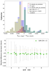 |
Fig. A.1. Top panel: Histogram distribution of the difference between the systemic redshift estimated from C III] performing a single-Gaussian fit (zsys, single) or a double-component fit (zsys, double). The blue histogram is the sum of all galaxies with C III] detected at S/N ≥3. The yellow and green histograms represent the subsets where the best-fit flux ratio between the two components of the double-Gaussian fit reaches one of the two extremes (respectively 1 and 0.625). The red histogram, from which we derive the correction of 26.25 km/s for the systemic redshift estimated through a single-Gaussian fit, includes galaxies with a best-fit ratio within the allowed range. Bottom panel: Velocity difference between the systemic redshift estimated from a single-Gaussian and a double-Gaussian fit of the C IIIλλ1907-1909 doublet, from Monte Carlo simulations, as a function of the S/N of the C III] line. The horizontal green dashed line represents the median difference for the simulated dataset. |
A.2. Comparison of the systemic redshifts estimated through CIII] and HeII
In this section, we compare the velocity shift vIS,comb, representative of low-ionisation absorption lines and available for the largest number of galaxies, estimated assuming the systemic redshift derived from the C IIIλλ1907-1909 line and from He II, for a subset of 18 galaxies where both emission lines are well fitted and detected with a S/N larger than 3. We remind that for all these cases we adopt the value inferred from C III] as our final estimate. The result of this comparison is shown in Fig. A.2. We can see that, assuming the He II as systemic redshift indicator, would produce no systematic biases in the final value of vIS,comb, and the 1σ scatter of the relation is consistent with the typical uncertainties of individual ISM-shift measurements. A similar behaviour is also found when comparing the ISM shift of individual lines (including also Al III and Si IV) estimated using C III] or He II line for the systemic redshift.
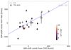 |
Fig. A.2. Comparison between the combined ISM-shift (i.e. for lower ionisation lines) estimated assuming the C III] as the systemic redshift indicator (x-axis) and the He II line (y-axis), for the sample where we obtain a reliable measurement of both lines with a S/N ≥3. The 1:1 relation is indicated with a blue dashed line, while the best-fit relation for our galaxies is indicated with black empty squares and black error bars. The data points are colour coded according to the S/N of the CIII] line. |
We know that the strong winds produced by Wolf-Rayet (WF) stars can broaden the He II line and induce an additional shift compared to the systemic redshift (Shirazi & Brinchmann 2012). However, as found in that paper, a significant contribution from these stars typically yields FWHM(He II) > 1000 km/s in galaxies, but these cases are excluded from our analysis, as explained in Section 2.2. We refer to Saxena et al. (2020) for a more complete treatment of the full sample of He II emitters in VANDELS.
A.3. Choosing the set of ISM lines for the combined fit
The large wavelength coverage of VANDELS spectra and the wide redshift range probed by the survey (2 < z < 6.5) allow us to study the ISM properties with multiple absorption lines in the UV regime. Most of these lines show similar properties in terms of velocity width and velocity shift with respect to the systemic redshift, hence it is reasonable to use them all together and perform a combined fit with a single redshift to increase the S/N of the final results. In order to decide which lines should be adopted in this combined fit, we first derive an average ISM redshift for each galaxy by fitting simultaneously all the ISM absorption lines that could be detected in the rest-frame range from 1216 Å to 2000 Å, namely Si IIaλ1260 Å, O I Si IIλλ1302-1304 Å, C IIλ1334 Å, Si IVλλ1394-1403 Å, Si IIbλ1526 Å, Fe IIλ1608 Å, Al IIλ1670 Å, and Al IIIλλ1855-1863 Å, as also listed in table 1. Given that we are studying individual lines before the combined fit, we apply here a detection threshold of 3 on the absorption lines, to increase the reliability of this test. We then compare these values to the redshift obtained for each individual absorption line used in the combined fit. Finally, for each line, we compute the fraction of galaxies where the corresponding redshift differs from the simultaneous fit value by more than 200 km/s. A higher fraction for a specific line would imply that its properties are different from the average of the other ISM lines, and thus it should be excluded from the combined procedure.
The outliers fraction foutliers for all the above ISM lines is presented in Fig. A.3. We can clearly see a segregation in this histogram: while foutliers is very low (below 5%) for half of the lines, it increases by a factor of three to ten for the other half of the list. Defining a maximum limit for the outliers fraction of 10% allows to isolate four lines, namely Si IIaλ1260 Å, C IIλ1334 Å, Si IIbλ1526 Å and Al IIλ1670 Å, that have likely similar properties and that we consider in this work for the combined fit.
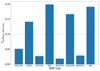 |
Fig. A.3. Fraction of galaxies for which the redshift measured from the single line fitting differs from the value obtained from a combined fit (including all the ISM lines detected in the spectrum) by more than 200 km/s, for each ISM line analysed in this paper. The horizontal line represents the fraction (10%) above which we have a significant number of outliers and the corresponding lines are not used in the combined fit. |
This choice is corroborated by a more detailed analysis of the entire set of ISM lines. Taking the SiII λ1526 Å as our reference, as it is available for the largest number of galaxies in our sample, we plot the ISM-shift derived for this reference line against that obtained with all the other lines, taking subsets of galaxies for which the two absorption features are both detected. The results of this exercise are shown in the figures A.4 and A.5. We can see that the four lines chosen for the combined fit are well aligned along the 1:1 relation with some scatter but no evident systematics (panels 1, 2, and 3).
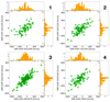 |
Fig. A.4. Comparison of the ISM velocity shift (in Km/s, referred to the systemic redshift) of the Si IV and Al III absorption lines for those galaxies in VANDELS where both features are detected with a S/N> 2. |
As far as the other lines are concerned, the O I Si IIλλ1302-1304 Å complex should be treated with caution. We performed a single Gaussian profile fit by considering the median of the doublet as the central wavelength (Fig. A.4- panel 4), and also a double Gaussian fit with a free-varying ratio between the two components. In both cases, we obtain ISM redshifts that are consistent with the global ISM value for part of the sample, but significantly lower for a large subset of objects, which causes the fraction of outliers to rise up to ∼14%, as shown in Fig. A.3. This might reflect the presence of two different species that contribute to the absorption complex, whose relative importance and properties are difficult to model, especially for individual systems where we are limited in S/N. For these reasons, we do not consider this absorption complex in the simultaneous fit.
The Fe IIλ1608 line has on average a positive velocity shift compared to the systemic redshift for this particular subset, as shown in Fig. A.5- panel 2, and we find a difference of ∼ + 150 km/s with respect to the ISM-shift of Si IIλ1526. This might suggest that the FeII line traces a gas component which is closer to the nucleus of the galaxy. As an alternative explanation, given that FeII is actually a blend of multiple hyperfine transitions of the same ionised element, there might be a non negligible contribution from transitions slightly longward of the main absorption at 1608.45 Å that is typically assumed also in other studies.
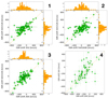 |
Fig. A.5. Comparison of the ISM velocity shift (in Km/s, referred to the systemic redshift) of the Si IV and Al III absorption lines for those galaxies in VANDELS where both features are detected with a S/N> 2. |
Finally, the Si IVλλ1394-1403 Å and Al IIIλλ1855-1863 Å doublets, which are representative of a gaseous component in a higher ionisation state, show on average more negative velocity shifts compared to the systemic redshift, indicative of higher velocity outflows by ∼150 km/s, hence we should treat them separately (Fig. A.5- panels 1 and 3). Moreover, these two lines share very similar properties, as the vIS that we measure from them are well correlated and remarkably in agreement with the 1:1 relation, without evident systematic errors (Fig. A.5- panel 4). This suggests that they might be powered by the same mechanism and emitted in the same regions.
All Tables
Absorption lines that we detected and fitted in this work, with their rest-frame wavelengths used for the derivation of the ISM velocity shifts.
Pearson correlation coefficients ρ (with corresponding p-values) between the ISM velocity shifts of low-ionisation lines and Si IV, and different physical properties of the galaxies that we analyse in this paper.
All Figures
|
Fig. 1. Systemic redshift distribution of galaxies with C III] or He II emission at S/N ≥ 3, selected in this work as described in the text. The green vertical lines represent the median redshift of the sample (continuous line) and the standard deviation of the distribution (dotted lines). |
| In the text | |
|
Fig. 2. Stack of all star-forming galaxies selected for our analysis (AGNs excluded). The green diamonds represent the pseudocontinuum points used for fitting the cubic spline to the stellar continuum. The red continuous line highlights the combined fit to the Si IIλ1260, Si IIλ1526, C IIλ1334, and Al IIλ1670 absorption lines, while the grey shaded regions have been masked in the fit. The vertical lines highlight the features used in the combined fit (in red), the absorption lines excluded from the combined fit but measured separately (in pink), and the emission lines used for the systemic redshift estimation (in green). |
| In the text | |
|
Fig. 3. Distribution of FWHM (in km s−1) for the sample selected in this work, for the following absorption lines detected with a S/N ≥ 2: Si IIa, O I Si II, Si IIb, C II, Fe II, Al II, Si IV, and Al III. The vertical lines highlight the median FWHM for each of the lines analysed. |
| In the text | |
|
Fig. 4. Distribution of ISM shift for the same lines shown in Fig. 3. Symbols and colours are the same as in the previous plot. The two dotted lines in addition to the dashed line of the median represent the standard deviation of vIS values. The number of galaxies contributing to each histogram is written in the top of each panel. |
| In the text | |
|
Fig. 5. Scatter plot comparing the ISM velocity shift of Si IIλ1526 to the FWHM of the same line (red diamonds). The black squares are the median vIS,Si II calculated in four bins of FWHM. In both cases, it is clear that there is no correlation between the two quantities. A similar result is also obtained for all the other absorption lines. |
| In the text | |
|
Fig. 6. Figure shows the spectrum of two galaxies at redshifts 2.587 and 3.479 in the UDS and CDFS field (top and bottom panels, respectively) with the combined fit of low-ionisation absorption lines (red), and for which we detect significant inflow signatures, with positive ISM velocity shifts as indicated in each panel (i.e. the centroids of ISM absorption lines are redshifted compared to the C III] centroid used for the systemic redshift). |
| In the text | |
|
Fig. 7. Spectral region around the ISM+stellar Si IV absorption doublet. In all the panels, the blue line is the stacked spectrum of all star-forming galaxies with C III] or He II emission selected in this work, where the error bars at each pixel represent the 1σ error. The orange line is the best-fit Gaussian made with MPFIT, assuming two Gaussian components for each side of the doublet (i.e. four Gaussians in total), as explained in the text. The red lines represent the best-fit models from Starburst99 (S99), Beagle (i.e. BC03 models), and BPASS, from top to bottom, respectively. The best-fit models have the closest stellar metallicity Z⋆ to the median of our galaxies (Calabrò et al. 2021), that is, log (Z⋆/Z⊙) = − 0.7 for S99, −0.82 for BC03, and −0.85 for BPASS. We reiterate the fact that the measured Z⋆ using BPASS calibrations is 0.1 dex lower than S99. |
| In the text | |
|
Fig. 8. Star-formation rate–stellar mass diagram for the sample of 330 C III] + He II emitters selected for our analysis. The main sequence relation by Speagle et al. (2014) is drawn with a black continuous line, while the dashed parallel lines represent the 1σ dispersion and the dotted line the starburst limit (4× above the main sequence). Our best-fit M⋆–SFR relation is represented with large red stars. On the y axis, we consider the SFR normalised to z = 3 assuming the evolving trend with redshift as (1 + z)2.8 from Sargent et al. (2012). |
| In the text | |
|
Fig. 9. HST F814W images (Koekemoer et al. 2011) of three galaxies with reliable systemic redshift and ISM-shift estimations. Upper row: these galaxies are visually identified as merging or interacting systems, as showing, from left to right, bridges connecting the interacting components, a very disturbed and asymmetric morphology, and a double nucleus. Bottom row: three examples of isolated or non-interacting galaxies with a discy shape (first case) and a more spheroidal structure (second and third image). |
| In the text | |
|
Fig. 10. Histogram distribution of the equivalent radius |
| In the text | |
|
Fig. 11. Upper panel: correlation of vIS,comb, vIS,Si IV and vIS,Al III with the stellar mass M⋆ for VANDELS star-forming galaxies selected in this work. The first two panels in each row show the relation for individual galaxies (red diamonds), while the black empty squares are the median vIS in bins of increasing M⋆. The red horizontal continuous line shows the median vIS for the entire sample shown in each plot, while the red shaded regions highlight the standard deviation of all the ISM shift values. The last panel of the row shows the velocity shifts calculated directly from the spectral stacks in four bins of stellar mass. Lower panel: same as above but as a function of the SFR. |
| In the text | |
|
Fig. 12. Diagrams comparing vIS,comb, vIS,Si IV and vIS,Al III to the equivalent radius |
| In the text | |
|
Fig. 13. Comparison of the line profiles in the spectral stack including all star-forming galaxies selected in this work (AGNs excluded). The central wavelengths resulting from a Gaussian fit are highlighted in cyan, blue, red, and dark red for the Si IIλ1526 line (representative of low-ionisation lines), Fe IIλ1608, Al IIIλλ1854-1862, and Si IVλλ1393-1402, respectively. |
| In the text | |
|
Fig. 14. Diagrams comparing vmax,comb and vmax,Si IV (estimated from stacked spectra) to other physical properties of the galaxies, namely the stellar mass M⋆, the SFR, the equivalent radius |
| In the text | |
|
Fig. 15. Dependence of the ISM velocity shift vIS on the merger flag (1 = mergers and 0 = non-mergers) and spectroscopic redshift. Each symbol represents a spectral stack in a different redshift or merger flag bin. The colours highlight the results from the combined fit of low-ionisation lines (black squares), Si IV (red circles), and the Al III absorption line (cyan triangles). |
| In the text | |
|
Fig. A.1. Top panel: Histogram distribution of the difference between the systemic redshift estimated from C III] performing a single-Gaussian fit (zsys, single) or a double-component fit (zsys, double). The blue histogram is the sum of all galaxies with C III] detected at S/N ≥3. The yellow and green histograms represent the subsets where the best-fit flux ratio between the two components of the double-Gaussian fit reaches one of the two extremes (respectively 1 and 0.625). The red histogram, from which we derive the correction of 26.25 km/s for the systemic redshift estimated through a single-Gaussian fit, includes galaxies with a best-fit ratio within the allowed range. Bottom panel: Velocity difference between the systemic redshift estimated from a single-Gaussian and a double-Gaussian fit of the C IIIλλ1907-1909 doublet, from Monte Carlo simulations, as a function of the S/N of the C III] line. The horizontal green dashed line represents the median difference for the simulated dataset. |
| In the text | |
|
Fig. A.2. Comparison between the combined ISM-shift (i.e. for lower ionisation lines) estimated assuming the C III] as the systemic redshift indicator (x-axis) and the He II line (y-axis), for the sample where we obtain a reliable measurement of both lines with a S/N ≥3. The 1:1 relation is indicated with a blue dashed line, while the best-fit relation for our galaxies is indicated with black empty squares and black error bars. The data points are colour coded according to the S/N of the CIII] line. |
| In the text | |
|
Fig. A.3. Fraction of galaxies for which the redshift measured from the single line fitting differs from the value obtained from a combined fit (including all the ISM lines detected in the spectrum) by more than 200 km/s, for each ISM line analysed in this paper. The horizontal line represents the fraction (10%) above which we have a significant number of outliers and the corresponding lines are not used in the combined fit. |
| In the text | |
|
Fig. A.4. Comparison of the ISM velocity shift (in Km/s, referred to the systemic redshift) of the Si IV and Al III absorption lines for those galaxies in VANDELS where both features are detected with a S/N> 2. |
| In the text | |
|
Fig. A.5. Comparison of the ISM velocity shift (in Km/s, referred to the systemic redshift) of the Si IV and Al III absorption lines for those galaxies in VANDELS where both features are detected with a S/N> 2. |
| In the text | |
Current usage metrics show cumulative count of Article Views (full-text article views including HTML views, PDF and ePub downloads, according to the available data) and Abstracts Views on Vision4Press platform.
Data correspond to usage on the plateform after 2015. The current usage metrics is available 48-96 hours after online publication and is updated daily on week days.
Initial download of the metrics may take a while.