| Issue |
A&A
Volume 667, November 2022
|
|
|---|---|---|
| Article Number | A9 | |
| Number of page(s) | 17 | |
| Section | Extragalactic astronomy | |
| DOI | https://doi.org/10.1051/0004-6361/202243406 | |
| Published online | 28 October 2022 | |
Unveiling the warm and dense ISM in z > 6 quasar host galaxies via water vapor emission⋆
1
Dipartimento di Fisica “G. Occhialini”, Università degli Studi di Milano-Bicocca, Piazza della Scienza 3, 20126 Milano, Italy
e-mail: This email address is being protected from spambots. You need JavaScript enabled to view it.
2
Dipartimento di Fisica e Astronomia, Alma Mater Studiorum, Università di Bologna, Via Gobetti 93/2, 40129 Bologna, Italy
3
INAF-Osservatorio di Astrofisica e Scienza dello Spazio, Via Gobetti 93/3, 40129 Bologna, Italy
4
Leiden Observatory, Leiden University, PO box 9513, 2300 RA Leiden, The Netherlands
5
Max-Planck-Institut für Astronomie, Königstuhl 17, 69117 Heidelberg, Germany
6
I. Physikalisches Institut, Universität zu Köln, Zülpicher Strasse 77, 50937 Köln, Germany
7
National Radio Astronomy Observatory, Pete V. Domenici Array Science Center, PO Box O, Socorro, NM 87801, USA
8
Max-Planck-Institut für Radioastronomie, Auf dem Hügel 69, 53121 Bonn, Germany
9
Steward Observatory, University of Arizona, 933 North Cherry Avenue, Tucson, AZ 85721, USA
Received:
23
February
2022
Accepted:
5
August
2022
Abstract
Water vapor (H2O) is one of the brightest molecular emitters after carbon monoxide (CO) in galaxies with high infrared (IR) luminosity, allowing us to investigate the warm and dense phase of the interstellar medium (ISM) where star formation occurs. However, due to the complexity of its radiative spectrum, H2O is not frequently exploited as an ISM tracer in distant galaxies. Therefore, H2O studies of the warm and dense gas at high-z remain largely unexplored. In this work, we present observations conducted with the Northern Extended Millimeter Array (NOEMA) toward three z > 6 IR-bright quasars J2310+1855, J1148+5251, and J0439+1634 targeted in their multiple para- and ortho-H2O transitions (312 − 303, 111 − 000, 220 − 211, and 422 − 413), as well as their far-IR (FIR) dust continuum. By combining our data with previous measurements from the literature, we estimated the dust masses and temperatures, continuum optical depths, IR luminosities, and star formation rates (SFR) from the FIR continuum. We modeled the H2O lines using the MOLPOP-CEP radiative transfer code, finding that water vapor lines in our quasar host galaxies are primarily excited in the warm, dense (with a gas kinetic temperature and density of Tkin = 50 K, nH2 ∼ 104.5 − 105 cm−3) molecular medium with a water vapor column density of NH2O ∼ 2 × 10¹⁷ − 3 × 1018 cm−3. High-J H2O lines are mainly radiatively pumped by the intense optically-thin far-IR radiation field associated with a warm dust component at temperatures of Tdust ∼ 80 − 190 K that account for < 5 − 10% of the total dust mass. In the case of J2310+1855, our analysis points to a relatively high value of the continuum optical depth at 100 μm (τ100 ∼ 1). Our results are in agreement with expectations based on the H2O spectral line energy distribution of local and high-z ultra-luminous IR galaxies and active galactic nuclei (AGN). The analysis of the Boltzmann diagrams highlights the interplay between collisions and IR pumping in populating the high H2O energy levels and it allows us to directly compare the excitation conditions in the targeted quasar host galaxies. In addition, the observations enable us to sample the high-luminosity part of the H2O–total-IR (TIR) luminosity relations (LH2O − LTIR). Overall, our results point to supralinear trends that suggest H2O–TIR relations are likely driven by IR pumping, rather than the mere co-spatiality between the FIR continuum- and line-emitting regions. The observed LH2O/LTIR ratios in our z > 6 quasars do not show any strong deviations with respect to those measured in star-forming galaxies and AGN at lower redshifts. This supports the notion that H2O can be likely used to trace the star formation activity buried deep within the dense molecular clouds.
Key words: galaxies: high-redshift / galaxies: ISM / quasars: emission lines / quasars: supermassive black holes
The reduced spectra and images reported in Figs. 2 and 3 are only available at the CDS via anonymous ftp to cdsarc.u-strasbg.fr (130.79.128.5) or via http://cdsarc.u-strasbg.fr/viz-bin/cat/J/A+A/667/A9
© A. Pensabene et al. 2022
 Open Access article, published by EDP Sciences, under the terms of the Creative Commons Attribution License (https://creativecommons.org/licenses/by/4.0), which permits unrestricted use, distribution, and reproduction in any medium, provided the original work is properly cited.
This article is published in open access under the Subscribe-to-Open model. This email address is being protected from spambots. You need JavaScript enabled to view it. to support open access publication.
1. Introduction
Quasars (or QSOs) at z > 6 are among the most luminous sources in the early Universe within the first billion years after the Big Bang. Their active galactic nuclei (AGN) are fueled by a rapid accretion of matter (> 10 M⊙ yr−1) onto a central supermassive black hole (BH; MBH ≳ 108 M⊙; see e.g., Jiang et al. 2007; De Rosa et al. 2011, 2014; Mazzucchelli et al. 2017; Schindler et al. 2020; Yang et al. 2021); while in their host galaxies, the impetuous consumption of huge gas reservoirs turns gas into stars at high rates (SFR > 100 M⊙ yr−1; see e.g., Bertoldi et al. 2003a,b; Walter et al. 2003; Walter 2009; Venemans et al. 2018, 2020). Their star formation activity is often enshrouded in large amounts of dust (Mdust ∼ 107 − 108 M⊙), making the host galaxies of z > 6 quasars very luminous in (far-)infrared (FIR) wavelengths (LFIR ∼ 1012 − 1013 L⊙) typical of the brightest nearby ultra-luminous IR galaxies (ULIRGs; see, e.g., Decarli et al. 2018; Venemans et al. 2018, 2020). Quasars cannot be merely considered a rare dramatic phenomenon but, rather, they constitute a fundamental phase in the formation and evolution of massive galaxies. For this reason, characterizing the quasar host galaxies at the highest redshifts is key to drawing insights on the interplay between star formation and BH accretion in shaping the galaxies from cosmic dawn to the contemporary Universe.
Recent decades have witnessed a veritable revolution with regard to the study of massive galaxies down to the Epoch of Reionization. The advent of sensitive facilities in the (sub-)mm bands, such as ALMA (Atacama Large Millimeter Array), as well as the recently upgraded IRAM/NOEMA (Institute de Radio Astronomie Millimétrique/Northern Extended Millimeter Array) have enabled astronomers to image the host galaxies of z > 6 quasars in unprecedented details. Bright tracers of the interstellar medium (ISM) such as the fine-structure line (FSL) of the singly ionized carbon [CII]158 μm, or carbon monoxide (CO) rotational lines at mid-/low-J (J ≲ 7), have been widely targeted to study the cold dense gas (Tgas < 100 K, nH2 ∼ 103 cm−3) morphology and kinematics (e.g., Walter et al. 2004, 2022; Maiolino et al. 2012; Wang et al. 2013; Cicone et al. 2015; Jones et al. 2017; Shao et al. 2017; Feruglio et al. 2018; Decarli et al. 2019; Neeleman et al. 2019, 2021; Venemans et al. 2019, 2020; Wang et al. 2019; Pensabene et al. 2020) in z > 6 quasars. The combination of FSLs from atomic neutral and ionized gas (e.g., neutral, and singly ionized carbon [CI], [CII], singly ionized nitrogen [NII], neutral, and doubly ionized oxygen [OI], [OIII]), and FIR transition from molecular gas phase (primarily CO rotational lines) have enabled characterizations of the physical properties of the multiphase ISM and to study its excitation conditions (e.g., Walter et al. 2003, 2018; Riechers et al. 2009; Gallerani et al. 2014; Venemans et al. 2017a,b; Carniani et al. 2019; Novak et al. 2019; Yang et al. 2019a; Herrera-Camus et al. 2020; Li et al. 2020a,b; Pensabene et al. 2021; Meyer et al. 2022). However, despite these efforts, further investigations are needed to shift toward a comprehensive view of the extreme conditions of the ISM in primeval quasar host galaxies. To this end, other tracers of the ISM probing different gas phases need to be targeted.
Among dense gas tracers, water vapor (H2O) is the strongest molecular emitter after high-J CO transitions in the ISM of IR-bright galaxies (see, e.g., Omont et al. 2013; Yang et al. 2016). The H2O lines are excited in shocked-heated regions, outflowing gas, and in the warm, dense molecular gas (nH2 ≳ 105 − 106cm−3, T ∼ 50 − 100 K; see González-Alfonso et al. 2010, 2012, 2013; van der Tak et al. 2016; Liu et al. 2017), where star formation ultimately occurs. Therefore, unlike other tracers traditionally used to study the dense gas (such as, e.g., high-J CO, 13CO HCO+, HCN, HNC), water vapor probes star-forming regions that are deeply buried in dust or heated gas in extreme environments of AGN. On the downside, the complexity of the H2O radiative spectrum implies that the excitation mechanism and the physical conditions of the ISM cannot be derived on the basis of the detection of a single or just a few lines (see, e.g., González-Alfonso et al. 2014; Liu et al. 2017). Both collisions and absorption of resonant radiation contribute to the excitation of H2O levels. In particular, IR radiative pumping is the main excitation mechanism of the high-J H2O lines (Weiß et al. 2010; González-Alfonso et al. 2014). This implies that water vapor emission provides us with insights on both the physical properties of the warm, dense medium, and on the IR radiation field. Interestingly, the intensity of H2O lines is found to be nearly linearly proportional with the total IR (TIR) luminosity of the galaxy (Omont et al. 2013; Yang et al. 2013, 2016; Liu et al. 2017).
Ground-based studies of water vapor emission in nearby galaxies are limited by telluric atmospheric absorption and consequently have been restricted to radio-maser transitions and a few transitions in luminous IR galaxies (e.g., Combes & Wiklind 1997; Menten et al. 2008). On the other hand, pioneering studies using the Infrared Space Observatory (Kessler et al. 1996) and Herschel (Pilbratt et al. 2010) have detected H2O emission (mainly in absorption) in local galaxies that are known to exhibit P-Cygni line profiles unambiguously associated with massive molecular outflows (e.g., Fischer et al. 1999, 2010; González-Alfonso et al. 2004, 2008, 2010, 2012; Goicoechea et al. 2005; van der Werf et al. 2010; Weiß et al. 2010; Rangwala et al. 2011; Sturm et al. 2011; Kamenetzky et al. 2012; Spinoglio et al. 2012; Meijerink et al. 2013; Pereira-Santaella et al. 2013; Liu et al. 2017; Imanishi et al. 2021). Water vapor emission have also been detected in starburst galaxies, Hy/ULIRGs, and quasars at higher redshifts (z ∼ 1 − 3; e.g., Bradford et al. 2011; Lis et al. 2011; Omont et al. 2011, 2013; van der Werf et al. 2011; Combes et al. 2012; Lupu et al. 2012; Bothwell et al. 2013; Yang et al. 2013, 2016, 2019b, 2020; Jarugula et al. 2019; Lehnert et al. 2020), up to z ≳ 6 − 7 (Riechers et al. 2013, 2017, 2021, 2022; Apostolovski et al. 2019; Koptelova & Hwang 2019; Yang et al. 2019a; Li et al. 2020b; Jarugula et al. 2021; Tripodi et al. 2022), where many FIR water transitions are redshifted in the ALMA and NOEMA bands. However, these sporadic water vapor detections primarily rely on one or two lines, thus leaving the warm and dense molecular ISM phase at z > 6 largely uncharted.
Given their large quantity of dust and extreme IR-luminosity, which can significantly enhance the emission from water vapor, z > 6 quasar host galaxies are thus ideal sources to target in their H2O lines. This paper is focused on the characterization of the warm, dense ISM and the local IR radiation field in three z > 6 quasar host galaxies: J2310+1855, J1148+5251, and J0439+1634. For these objects, [CII]158 μm, multiple CO lines, and other ISM probes (including sparse H2O lines) as well as a dust continuum were previously detected (Bertoldi et al. 2003a; Robson et al. 2004; Walter et al. 2004, 2009; Maiolino et al. 2005, 2012; Beelen et al. 2006; Riechers et al. 2009; Wang et al. 2011, 2013; Leipski et al. 2013; Gallerani et al. 2014; Cicone et al. 2015; Feruglio et al. 2018; Carniani et al. 2019; Hashimoto et al. 2019; Shao et al. 2019; Yang et al. 2019a; Li et al. 2020a,b; Yue et al. 2021; Meyer et al. 2022; Tripodi et al. 2022). Here, we present NOEMA 2-mm band observations toward J2310+1855, J1148+5251, and J0439+1634, targeted in their four ortho- and para-H2O rotational lines (312 − 303, 111 − 000, 220 − 211, and 422 − 413), together with the underlying FIR dust continuum. The targeted lines cover a wide range in H2O energy levels associated to different gas regimes. After combining information from such tracers, in conjunction with data retrieved from the literature, we performed radiative transfer analysis by employing the MOLPOP-CEP code (Asensio Ramos & Elitzur 2018). This enabled us to study the H2O excitation mechanisms and to put constraints on the physical properties of the warm, dense phase of the ISM and the local IR dust radiation field in quasar host galaxies at cosmic dawn.
This paper is organized as follows. In Sect. 2, we present our quasar sample and the NOEMA observations, and we describe the data processing. In Sect. 3, we outline the characteristics of H2O emission lines and their excitation mechanism. In Sect. 4, we describe the analysis of the calibrated data and we report the H2O line and FIR continuum measurements toward our three quasar host galaxies. In Sect. 5, we focus on the dust properties inferred from the analysis of the FIR dust continuum. In Sect. 6, we describe the setup of our radiative transfer models obtained with MOLPOP-CEP code. In Sect. 7, we compare our measurements with other studies in the literature and we present and discuss our results obtained by modeling the H2O lines. Finally, in Sect. 8, we summarize the results and present our conclusions. Throughout this paper we assume a standard ΛCDM cosmology with H0 = 67.7 km s−1 Mpc−1, Ωm = 0.307, ΩΛ = 1 − Ωm from Planck Collaboration XIII (2016).
2. Observations and data reduction
The goal of this work is to capitalize on multiple H2O lines in order to unveil their excitation mechanisms and to characterize the warm and dense molecular ISM and the local dust IR radiation field in a sample of z > 6 IR-bright quasar host galaxies. For these purposes, the quasars J2310+1855 (z = 6.00), J1148+5251 (z = 6.42), and J0439+1634 (z = 6.52) are ideal targets visible from the NOEMA site. They are among the IR-brightest of all known quasars at z ≳ 6. For this reason, on the basis of the observed (almost linear) correlation between H2O and IR luminosities (Yang et al. 2013; Liu et al. 2017), they are expected to have bright H2O lines. In addition, they have been previously detected in some H2O lines (Yang et al. 2019a; Li et al. 2020a, and Riechers et al. in prep.) that we use here to complement our analysis. We note that the J0439+1634 is a lensed source with a host galaxy magnification factor in the range of 2.6–6.6 (95% confidence interval, see Fan et al. 2019; Yang et al. 2019a; but see also Yue et al. 2021 for a detailed analysis on high-angular resolution [CII] ALMA observations). However, as also reported by Yang et al. (2019a), all our observed H2O lines in J0439+1634 are fit well by a single Gaussian profile (see Sect. 4), thus suggesting that a contribution from differential lensing affecting the kinematics structure of the source is likely to be minor (see, e.g., Rivera et al. 2019; Yang et al. 2019b). All the quantities reported in this work for J0439+1634 are intended as purely observed quantities (unless otherwise specified). We summarize the properties of our sample in Table 1. We observed the targeted quasars using the IRAM/NOEMA interferometer in compact (C or D) array configuration (project ID: S19DL). The PolyFix band 2 receivers was tuned to secure the 1080–1130 GHz and 1190–1245 GHz rest-frame frequency windows in the lower (LSB) and upper side bands (USB), respectively.
The sample of quasars studied in this work.
The quasar J2310+1855 was observed in two tracks on October 12 and November 10, 2019. The blazar 3C454.3 was observed as phase and amplitude calibrator, while the absolute flux scale and the bandpass were set by observing the MWC349 calibrator. The precipitable water vapor (PWV) column density was 8 − 10 mm in the October track and 4 − 6 mm in the November one. The quasar J1148+5251 was observed on September 09, 2019. We observed the sources 3C84 and LKHA101 as flux and bandpass calibrators. The PWV during the observations was 2 − 6 mm. Finally, J0439+1634 was observed on August 09, 13, and 14, 2019. The sources 3C84, 3C454.3, MWC349, and LKHA101 were used as flux and bandpass calibrators, while the radio-loud quasar 0446+112 acted as phase and amplitude calibrator. The PWV was 8 − 12 mm in the first visit, and 2 − 4 mm in the other tracks.
We used the CLIC software in the GILDAS suite (February 2020 version) to reduce and calibrate the data. The high PWV and consequently high system temperature (> 200 K at the tuning frequencies) led to poor phase rms residuals in the August 09, 13 and October 12 tracks, which were thus flagged out. The calibrated cubes have 8726, 9090, and 6690 visibilities for J2310+1855, J1148+5251 and J0439+1634, respectively, corresponding to 3.0, 3.2, and 2.3 h on source (a nine-antennas equivalent).
We adopted the MAPPING software in the GILDAS suite to invert the visibilities and image the cube. The half power primary beam width is 29.2″, 31.0″, and 31.4″ at the tuning frequencies of the three quasars (172.443 GHz, 162.776 GHz, and 160.612 GHz for J2310+1855, J1148+5251, and J0439+1634, respectively). Using natural weighting of the visibilities, we obtain synthesized beams of 1.47″ × 0.79″, 2.45″ × 2.13″, and 2.81″ × 2.51″, respectively. We resampled the cubes adopting a channel width of 50 km s−1. The achieved median RMS per channel in the LSB and USB respectively are 0.61 mJy beam−1 and 1.50 mJy beam−1 for J2310+1855, 0.42 mJy beam−1 and 0.60 mJy beam−1 for J1148+5251, and 0.52 mJy beam−1, 0.66 mJy beam−1 in the case of J0439+1634.
3. The H2O emission lines and their excitation
In Fig. 1, we show the ladder structure of the H2O molecule (limited to energy levels < 500 K). In the figure we indicate the H2O transitions targeted in our NOEMA program together with the additional lines reported in the literature for our three targeted quasars. Properties of the relevant transitions, such as the energy of the upper levels (Eup), the rest frequencies (νrest), and the Einstein A coefficients for spontaneous emission, are summarized in Table 2.
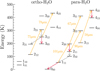 |
Fig. 1. Energy level diagram of H2O. Downward solid red and gray arrows are the transitions reported in this paper and those available in the literature (see Yang et al. 2019a, Li et al. 2020b, Riechers et al., in prep.). The upward dashed orange arrows indicate the FIR H2O pumping (absorption) lines of interest. The respective wavelengths are also reported. |
List of the targeted H2O emission lines in quasars.
The excitation of the water vapor molecule is very sensitive to the physical conditions of the line-emitting region. As revealed by previous studies (e.g. González-Alfonso et al. 2012, 2014; Liu et al. 2017), low-level transitions (Eup < 250 K) arise in warm collisionally excited gas with kinetic temperature of Tkin ∼ 30 − 50 K, and clump density of nH ≳ 105 cm−3 that drives the low-level populations toward the Boltzmann distribution, with excitation temperature equal to the gas kinetic temperature (Tex ≃ Tkin). This may occur even in environments with molecular gas density well below the critical density (ncrit ∼ 107 − 109 cm−3, e.g., Faure et al. 2007), due to the large optical depth of such H2O lines and radiative trapping effect that lowers the effective density at which the lines appear to be thermalized (see, e.g., Poelman et al. 2007). The high-lying H2O lines instead require radiative excitation by far-IR photons from warm dust (Tdust ∼ 70 − 100 K) that are then re-emitted through a fluorescence process. This is illustrated in Fig. 1 where we report six far-IR pumping transitions (58 μm, 67 μm, 75 μm, 78 μm, 90 μm, 101 μm) that account for the radiative excitation of some sub-mm lines. Interestingly, the low-excitation lines (Eup < 150 K) are predicted to become weaker or completely disappear under the continuum level for increasing the dust temperature (e.g., Liu et al. 2017). In particular, the para-H2O ground state transition 111 − 000 is not involved in any IR-pumping cycle and its flux is predicted to be negligible in regions where the IR pumping dominates. Indeed, the upper level 111 can be populated only by absorption of the line photon at 269 μm, or by a collisional event. This implies that in absence of significant collisional excitation (i.e., low gas density) the H2O 111 − 000 line will be mainly detected in absorption in case of significant 269 μm continuum opacity (e.g., González-Alfonso et al. 2004; Rangwala et al. 2011). On the other hand, in warm and dense gas regions with low continuum opacity, the ground state transition is expected to be detected in emission. In this case, the 111 level will be significantly populated by collisions, thus enhancing the IR pumping cycle by absorption of 101 μm photons and boosting the J = 2 para-H2O lines.
As part of our NOEMA program, we detected up to three para- and ortho-H2O lines in each quasars that we complemented with other J = 2, and J = 3 H2O lines from the literature (Yang et al. 2019a; Li et al. 2020b, Riechers et al., in prep.; see Table 3). This data set allows us to cover a wide range of energy of H2O levels (50 K < Eup < 500 K), thus enabling for the first time a comprehensive analysis of the H2O energetics in these high-z quasars.
Measurements and derived quantities of the NOEMA spectra of the quasars.
4. Line and continuum measurements
Since our sources are not spatially resolved in the observations, we obtained the beam-integrated spectra by performing single-pixel extraction at the nominal coordinates of the targets (see Table 1) from the data-cubes including the continuum emission. We then performed spectral fitting with a composite model that includes a single Gaussian component for the line and a constant for the continuum. We sampled the parameter space by using the package emcee (Foreman-Mackey et al. 2013), namely, a Markov chain Monte Carlo (MCMC) ensemble sampler developed in Python. This procedure allows us to effectively sample the posterior probability space. As data uncertainties in the likelihood estimates, we assume the 1-σ Gaussian RMS of each imaged channel, and we neglect any systematic term. We therefore obtained the posterior probability distributions of the free parameters from which we derived the line and continuum measurements by computing the 50th percentile as the nominal values, and the 16th and 84th percentile as 1-σ statistical uncertainties. We then derived the line luminosities as (see, e.g., Solomon et al. 1997):
![Mathematical equation: $$ \begin{aligned}&L_{\rm line}\,[L_{\odot }] = 1.04\times 10^{-3}\,S\Delta { v}\,\nu _{\rm obs}D_{\rm L}^2\,, \end{aligned} $$](/articles/aa/full_html/2022/11/aa43406-22/aa43406-22-eq54.gif) (1)
(1)
![Mathematical equation: $$ \begin{aligned}&L^\prime _{\rm line}\,[\mathrm{K\,km\,s^{-1}pc^2}] = 3.25\times 10^7\,S\Delta { v}\frac{D_{\rm L}^2}{(1+z)^3\,\nu _{\rm obs}^2}, \end{aligned} $$](/articles/aa/full_html/2022/11/aa43406-22/aa43406-22-eq55.gif) (2)
(2)
where SΔv is the velocity-integrated line flux in Jy km s−1, νobs is the observed central frequency of the line in GHz, and DL is the luminosity distance in Mpc. The relation between Eq. (1) and (2) is  . We show the spectra of the sources with the best-fit models in Fig. 2 and we report the derived quantities in Table 3 together with the additional H2O line detections from the literature. In Fig. 3, we show the continuum-subtracted line velocity-integrated maps, where the latter are obtained by averaging the continuum-subtracted cubes over 1.2 × FWHM around the line. This velocity range is expected to maximize the S/N assuming an ideal Gaussian line profile and constant noise over the spectral channels. Throughout the text, we report the significance on the measured line fluxes in unit of
  , where Δv is the channel width (50 km s−1), FWHM is the full width at half maximum of the best-fit Gaussian line model (in km s−1), and the ⟨rms⟩ is the median rms noise of the line cube (see Sect. 2). In cases where line emission is not detected, we report 3σ upper limits, assuming a source-specific FWHM value computed as the inverse-variance-weighted mean of the measured FWHM of the detected lines.
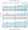 |
Fig. 2. NOEMA spectra of the three z > 6 quasars J2310+1855, J1148+5251 and J0439+1634 (from top to bottom). We report the observed data in light blue and the best-fit models in red. The blue dashed lines indicate the rest frequencies of the targeted H2O transitions (quantum numbers are also reported). At the bottom of each spectra, we report the residuals (data-model). The gray-shaded areas show the noise RMS across the spectra. |
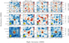 |
Fig. 3. Continuum-subtracted line velocity-integrated maps of the quasars J2310+1855, J1148+5251, J0439+1634 (from top to bottom). Yellow crosses indicate the nominal coordinate of the source. The synthesized beam FWHM is reported at the bottom-left corners. The line maps are obtained by integrating over 1.2 × FWHM around the line central frequency. The black contours give the [ − 4, −2, 2, 3, 4, 5, 6, 7, 8, 16, 32]σ isophotes. Negative contours are shown as dotted lines. |
5. Dust properties from FIR continuum
The far-infrared continuum flux densities are key measurements to constrain the dust physical properties of galaxies. At (sub-)mm wavelengths the observed flux of z > 6 quasar host galaxies is dominated by the dust re-emission of (rest-frame) UV photons from stars and the central AGN (e.g., Beelen et al. 2006; Leipski et al. 2013, 2014). The interstellar dust grains absorb and emit radiation with an efficiency that depends on the wavelength of the incident photons (Draine & Lee 1984) and, therefore, they do not behave as an ideal blackbody. The dust IR flux density at the rest-frame frequency ν emitted by a galaxy can be described by the dubbed “graybody” law: Sν ∝ (1 − e−τν)Bν(Tdust), where Bν(Tdust) is the Planck function depending on the dust temperature (Tdust), and τν is the frequency-dependent dust optical depth. The observed flux density at frequency ν/(1 + z) from a source at redshift z can be expressed in terms of the dust mass (Mdust) as (see, e.g., Carniani et al. 2019; Liang et al. 2019):
 (3)
(3)
where κν being the mass absorption coefficient, and DL is the redshift-dependent luminosity distance. The above equation provides us with a useful formula to estimate the dust mass and temperature from the observed (sub-)mm continuum flux densities. However, Eq. (3) depends on largely unknown parameters such as the dust optical depth, τν, and the dust mass absorption coefficient, κν that are difficult to determine. Indeed, observational studies at low and high redshifts have shown that the interstellar dust emission becomes optically thick at wavelengths around λrest = 50 − 200 μm (e.g., Blain et al. 2003; Conley et al. 2011; Rangwala et al. 2011; Riechers et al. 2013; Simpson et al. 2017; Carniani et al. 2019; Faisst et al. 2020). However, the strong contribution of AGN torus at MIR wavelengths has prevented us from reliably sampling the Wien’s tail of the dust SEDs in J2310+1855 and J1148+5251 (see, e.g., Leipski et al. 2014; Shao et al. 2019), and in the case of J0439+1634, we lack continuum detections at (rest frame) < 100 μm, which is where the effect of dust optical depth is expected to be important. We therefore adopted the mass absorption coefficients for standard ISM from Draine (2003). We then extrapolated κν at any frequency in the (rest-frame) range 6 − 1000 μm via a linear interpolation of the tabulated data, and we parametrized the continuum optical depth as τν = τ100κν/κ100, where τ100, and κ100 are the continuum optical depth and the dust mass absorption coefficient at (rest frame) 100 μm, respectively.
The observed flux of Eq. (3) must be corrected for the effect of the cosmic background radiation (CMB), the temperature of which is TCMB(z = 6)≈19 K. In such conditions, the CMB acts a strong background source that attenuates the observed flux density and provides a thermal bath heating the dust. da Cunha et al. (2013, see also Zhang et al. 2016) show that the recovered dust continuum observed against the CMB is given by:
 (4)
(4)
![Mathematical equation: $$ \begin{aligned}&{T_{\rm dust}(z)=\left\{ \!\left( T_{\rm dust}^{z=0} \right)^{4+\beta }+\!\left( T_{\rm CMB}^{z=0} \right)^{4+\beta }\left[ \!\left( 1+z \right)^{4+\beta }-1 \right] \right\} ^{1/(4+\beta )}, } \end{aligned} $$](/articles/aa/full_html/2022/11/aa43406-22/aa43406-22-eq60.gif) (5)
(5)
where  and
and  are the corresponding dust and CMB temperatures at z = 0, and β is the dust spectral emissivity index. Throughout the rest of the paper, we use Tdust to indicate the “actual” dust temperature, namely, Tdust(z), including the contribution to the dust heating provided by the CMB (as in Eq. (5)). The quasars J2310+1855 and J1148+5251 have been widely studied in literature, and for these sources, the dust physical properties are generally constrained using different SED decomposition models (see, e.g., Leipski et al. 2013, 2014; Shao et al. 2019). However, here we aim to obtain quasar dust properties by adopting the same method for all the sources. For this purpose, we combined our continuum measurements in J2310+1855, J1148+5251, and J0439+1634 (see Table 3) with the available continuum flux density measurements from the literature (see Fig. 4) in the range of λrest ≈ 50 − 1000 μm, where the dust emission is expected to be powered primarily by the re-processed optical/UV radiation of young stars in star-forming regions thus avoiding the MIR excess due to the AGN torus contribution or very hot dust components (Casey 2012; Leipski et al. 2013, 2014; Casey et al. 2014). Shao et al. (2019) and Leipski et al. (2014) have shown that the AGN in J2310+1855 and J1148+5251 starts to dominate the FIR flux at (rest-frame) wavelengths < 50 μm, thus providing a significant contribution (up to ∼50%, depending on the details of the SED modeling) to the total IR luminosity. For the purposes of this work, our aim is to obtain the FIR luminosity contribution from the ISM dust emission only, which is directly linked to the excitation of H2O lines and which provides us with SFR estimate. This also allow us to perform a fair comparison with IR luminosities of other samples of star-forming galaxies and AGN.
 |
Fig. 4. Infrared dust continuum SED modeling of J2310+1855 (yellow), J1148+5251 (blue), and J0439+1634 (red). The upper-left panel shows continuum data retrieved from the literature derived for the wavelength range λrest ≈ 50 − 1000 μm and our NOEMA 2-mm continuum measurements (see the legend). The solid curves are the best-fit models to the observed data while shaded areas indicate the 1-σ confidence intervals. The green band is the 2-mm wide-band of the NOEMA PolyFix correlator scaled to the quasar rest frame wavelengths using the average redshift of the quasars. The adjacent panels show the posterior probability distribution of the dust SED model (free) parameters. The best-fit values and uncertainties are reported at the top of the distributions and they are defined as the 50th, 16th, and 84th percentiles. The 2D contours show the [1, 2, 3]σ confidence intervals that are also highlighted in the marginalized distributions. References. Bertoldi+03 (Bertoldi et al. 2003a); Robson+04 (Robson et al. 2004); Beelen+06 (Beelen et al. 2006), Riechers+09,+ (Riechers et al. 2009, Riechers et al. in prep.); Walter+09 (Walter et al. 2009); Wang+11,+13 (Wang et al. 2011, 2013); Leipski+13 (Leipski et al. 2013); Gallerani+14 (Gallerani et al. 2014); Cicone+15 (Cicone et al. 2015); Feruglio+18 (Feruglio et al. 2018); Carniani+19 (Carniani et al. 2019); Hashimoto+19 (Hashimoto et al. 2019); Shao+19 (Shao et al. 2019); Yang+19 (Yang et al. 2019a); Li+20a,+20b (Li et al. 2020a,b); Meyer+22 (Meyer et al. 2022). |
Therefore, we used Eqs. (3) and (4) to fit the dust SEDs of our quasars by using Tdust, Mdust, and τ100 as free parameters. We explored the parameter space by adopting a Bayesian approach via the MCMC ensemble sampler emcee (Foreman-Mackey et al. 2013). In this procedure, we treated the continuum data as independent measurements with Gaussian statistical uncertainties and ignoring any systematics. We adopted shallow box-like priors on free parameters as follows: TCMB(z)≤Tdust ≤ 150 K, 6.0 ≤ log Mdust ≤ 10.0, and 0.01 ≤ τ100 ≤ 150 in line with the typical values observed in high-z star-forming galaxies and quasars (e.g., Beelen et al. 2006; Leipski et al. 2013, 2014). In the case of J0439+1634, the available data are limited to the Rayleigh-Jeans (RJ) tail of the dust SED, where the observed flux density is ∝TdustMdust, thus making these parameters degenerate. In addition, the lack of data at shorter wavelengths leaves τ100 unconstrained. In order to fit the dust SED of J0439+1634, we therefore included a Gaussian prior on Tdust in the log-likelihood function of the form −0.5{(Tdust − 70 K)/(15 K)}2, with 70 K being the typical dust temperature independently found by Carniani et al. (2019) for J1148+5251 and J2310+1855, and taking into account the dust optical depth. We show the fit results in Fig. 4. We then derived rest-frame FIR luminosities (42.5 − 122.5 μm, 40 − 400 μm; see Helou et al. 1985, 1988) and TIR (8 − 1000 μm, Sanders et al. 2003) luminosities of the sources by integrating the best-fit models in the corresponding frequency range. Finally, we inferred the SFR by using the local scaling relation from Murphy et al. (2011); SFRIR(M⊙ yr−1) = 1.49 × 10⁻¹⁰ LTIR/L⊙, under the hypothesis that the entire Balmer continuum (i.e., 912 Å < λ < 3646 Å) is absorbed and re-irradiated by the dust in the optically thin limit. Here, a Kroupa initial mass function (IMF; Kroupa 2001) is implicitly assumed, having a slope of −1.3 for stellar masses between 0.1 − 0.5 M⊙, and −2.3 for stellar masses ranging between 0.5 − 100 M⊙. In Table 4, we report all the derived quantities obtained with our dust continuum modeling. We note that under our working assumptions, any possible contribution of the central AGN to the IR luminosity will result in biases on derived quantities, in particular, an overestimation of IR luminosities and the SFRIR.
Dust properties in quasar host galaxies.
The estimated dust temperature in both quasar host galaxies J2310+1855 and J1148+5251 is higher than that derived by Shao et al. (2019) and Leipski et al. (2013, 2014), who performed quasar SED decomposition in the UV/optical-FIR range. Also, in the case of J1148+5251, we find a higher Tdust value compared to other works at FIR wavelengths (Cicone et al. 2015; Meyer et al. 2022). In general, our Tdust values are higher than typical dust temperature measured in high-z quasar hosts (e.g., Beelen et al. 2006; Wang et al. 2007, 2008; Leipski et al. 2013, 2014). However, the aforementioned studies typically assume optically thin dust emission and κν ∝ νβ, with a dust emissivity index β = 1.6. On the other hand, we found values of Tdust and Mdust that are consistent within 2σ with those found by Carniani et al. (2019), which takes into account the effect of the continuum optical depth. Indeed, our results point to optical thick conditions at < 100 μm in all the cases. However, we note that the derived dust parameters from SED fitting depend on the adopted functional form as well as the broad-band photometry used in the fit. Indeed, a single-temperature modified blackbody cannot account for the superimposed emission from multiple dust components in galaxy. In general, the contribution to the TIR luminosity in the RJ regime of the dust SED is expected to be dominated by the vast cold dust reservoir (T ∼ 20 K), while warmer dust components (T ≳ 50 − 60 K) boost the IR-luminosity at shorter wavelengths (e.g., Dunne & Eales 2001; Farrah et al. 2003; Casey 2012; Galametz et al. 2012; Kirkpatrick et al. 2012, 2015). The luminosity on RJ regime is only linearly proportional to the dust temperature, while LFIR scales much faster near to the peak of the dust SED. For this reason, the presence of a warmer dust component may significantly bias our single-component modeling toward higher dust temperatures, even if the warm dust is a small fraction of the total dust mass. However, the available continuum measurements of our quasars hosts do not allow us to measure the potential small secondary peak associated to the cold dust on the RJ tail of the SED. Therefore, our dust temperature estimates should be considered as “luminosity-weighted” in contrast to the “mass-weighted” dust temperature physically associated to the bulk of the cold dust emission in galaxies (see, e.g., Scoville et al. 2016; Behrens et al. 2018; Liang et al. 2019; Faisst et al. 2020; Di Mascia et al. 2021; Sommovigo et al. 2021; as well as Harrington et al. 2021 for further discussion).
6. Radiative transfer analysis
The observed line and continuum luminosities incorporate key information on the physical properties of the emitting regions. Such information can be extracted by a forward modeling of the observed quantities under a number of simplified assumptions on the geometry of the emitting region and on the atomic or molecular excitations and radiative transfer processes. In this work, we adopt the publicly-available radiative transfer code MOLPOP-CEP1 (Asensio Ramos & Elitzur 2018) in order to simulate the emission of H2O lines from a molecular cloud under the effect of a dust radiation field. Compared to other methods, this code solves “exactly” (i.e., in principle, at any level level of accuracy), the radiative transfer equations for a multi-line problem via the coupled escape probability approach (CEP, Elitzur & Asensio Ramos 2006) in the case of a one-dimensional (1D) plane-parallel slab of gas that can present arbitrary spatial variations of the physical conditions. This code divides the source in a set of zones in which the level population equations are derived from first principles and solved self-consistently including interactions with the transferred radiation and (possibly) an external radiation field. Therefore, the emergent line fluxes are predicted as a function of the depth into the line-emitting region that can be directly compared with the observations. This level of sophistication is necessary since we are dealing with radiative transfer under very optically thick conditions, both in the continuum and in the lines.
Within MOLPOP-CEP we studied the water vapor emission lines by setting up uniform slab models of molecular cloud impinged by an external radiation field produced by the dust. The parameters of interest for the molecular system are: the density of molecular hydrogen (nH2), the kinetic temperature of the gas (Tkin), the water abundance (XH2O), and the H2O column density (NH2O). We characterized the external dust radiation field by adopting a single modified black body model of the form (1 − e−τν)Bν(Tdust) impinging the molecular medium from a side. The radiation field is therefore determined by the dust temperature (Tdust), and the continuum optical depth at each frequency (τν). In addition, we take into account the effect of CMB at z ∼ 6 by inserting a blackbody radiation field with temperature of TCMB = 19.08 K illuminating the molecular slab from both sides.
In order to model the H2O emission in our quasar host galaxies, we assumed fiducial values of Log nH2 (cm−3) = 4.5, Tkin = 50 K, and XH2O = 2 × 10⁻⁶ (see, e.g., Meijerink & Spaans 2005; González-Alfonso et al. 2010; Liu et al. 2017; van Dishoeck et al. 2021). We therefore generated a 16 × 25 grid of models with different dust radiation fields by varying the dust temperature in the range of Tdust = [45, 195] K (with 10 K linear spacing) and continuum optical depth at 100 μm in the range of τ100 = [0.01, 150] (∼0.17 dex spacing). The continuum optical depth at every wavelength is then determined by a tabulation available within the code, corresponding to the properties of standard ISM dust (see Asensio Ramos & Elitzur 2018). For para- and ortho-H2O collisional excitations we assume both ortho- and para-H2 molecules as collisional partners by adopting collisional rate coefficients from Daniel et al. (2011). The radiation field impinges the molecular system and the code computes the radiation transfer all the way into the cloud until the water vapor column density reaches NH2O = 1 × 1019 cm−2 (NH2 = 5 × 1024 cm−2). The allowed range of the various parameters are set in order to encompass the typical values observed in local and high-z galaxies (see, e.g., van der Werf et al. 2011; González-Alfonso et al. 2014; Yang et al. 2016, 2020; Liu et al. 2017; Pensabene et al. 2021). Following the prescriptions reported in Asensio Ramos & Elitzur (2018), we set up the calculations by dividing the molecular cloud into 20 zones, achieving a relative accuracy in the solution of the non-linear level population equations of < 0.01 with the accelerated Λ-iteration method (ALI).
The models adopted in this work are suitable to simulate the emission of a typical molecular cloud in a galaxy. The simplified assumptions make these models undoubtedly less adequate to provide a realistic picture of the complex ISM conditions in galaxies. In particular, our model is based on one-dimensional slabs with no defined volume. Therefore, our model cannot provide us with volume-integrated quantities (e.g., total IR luminosities, total line fluxes, molecular mass, etc.). We also note that a comprehensive modeling of water vapor emission should include the contribution of multiple gas and dust components in order to perform a fairer modeling of the collisionally excited low-J and radiatively excited high-J H2O lines simultaneously (see, e.g., González-Alfonso et al. 2010; van der Werf et al. 2011; Liu et al. 2017; Yang et al. 2020; see also Riechers et al. 2022). Specifically, a cold (extended) gas component associated with the collisional excitation of the low-lying H2O lines mainly driven by the gas density and temperature, and (at least) one warm or hot (compact) component responsible for the radiative excitation of high-J H2O transitions that are mainly sensitive to the dust temperature. However, we verified that our current data do not enable us to constrain the gas temperature and density such that any multicomponent approach would be inconclusive. This drives our analysis strategy consisting in a single gas and dust component assuming fiducial values of the gas density, temperature, and water vapor abundance (as discussed above).
7. Results and discussion
7.1. H2O spectral line energy distributions
In order to investigate the excitation of the H2O lines we study the spectral line energy distribution (SLED), that is, the water vapor line ratios as function of the energy of the upper level of transitions (Eup). In Fig. 5, we compare the H2O (312 − 303)-normalized SLEDs (using line velocity-integrated fluxes in unit of Jy km s−1) in our quasars, with the average SLEDs of local ULIRGs, including cases with mild AGN contribution (“HII+mild AGN”), and AGN-dominated galaxies (“strong-AGN”) as reported by Yang et al. (2013). In order to extend the comparison, in Fig. 5, we also report three detailed H2O SLED available in the literature, for the local Type-1 Seyfert galaxy Mrk 231 (González-Alfonso et al. 2010), the local ULIRG Arp 220 (Rangwala et al. 2011), and the SMG HFLS 3 at z = 6.34 (Riechers et al. 2013). To the first order (within the measurement uncertainties), our quasars show H2O SLEDs that resemble the ones of other high-z galaxies (with or without prominent AGN).
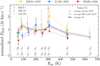 |
Fig. 5. H2O (312 − 303)-normalized intensities (in Jy km s−1) as a function of the energy of the upper levels. Colored diamonds are the H2O line ratios of our three quasars as indicated in the legend at the top of the panel. The red and blue dotted lines are, respectively, the average H2O SLED of local strong-AGN- and HII+mild-AGN-dominated galaxies reported in Yang et al. (2013). The solid black line is the average SLED of the whole sample with the gray shadowed area representing the 1-σ uncertainty. We also report data retrieved from the literature for the nearby ULIRG Arp 220 (Rangwala et al. 2011), the AGN-dominated galaxy Mrk 231 (González-Alfonso et al. 2010), and the SMG HFLS 3 at z = 6.34 (Riechers et al. 2013). The energy of upper levels of 202 − 211 and 312 − 303 transitions were shifted for clarity to −15 K and +25 K, respectively. We also slightly shifted the SLEDs of Arp 220, Mrk 231, HFLS 3 horizontally to −5 K, and those of our quasars to +5 K for clarity. |
More specifically, Yang et al. (2013) report a high detection rate of H2O 111 − 000 in luminous AGN, possibly indicating strong H2O collisional excitation due to the high density gas in the AGN circumnuclear region (see discussion in Sect. 3). However, we detected the para-H2O ground state transition only in quasar J1148+5251. In accordance with the discussion in Sect. 3, this may suggest that the bulk of the H2O emission in this source arises from a warm ISM with low continuum opacity. At the same time, J1148+5251 is the only one source in our sample that is not detected in its H2O 422 − 413 transition. This might point to a weaker contribution of the warm dust in J1148+5251, compared to the other two sources.
In particular, H2O 321 − 312 is the brightest observed H2O line in most of our quasar host galaxies. This is especially evident for J2310+1855, which shows a peak in the H2O SLED at the position of this line as in the average local SLED of ULIRGs and AGN. The H2O 321 level is indeed not only approximately thermalized by collisions in the warm medium, but also efficiently populated by absorption of 75 μm photons of the warm dust (e.g., Liu et al. 2017). In addition, in optically thin conditions, every de-excitation in H2O 321 − 312 line will be followed by a cascade either in the H2O 312 − 303 or 312 − 221 transition (see Fig. 1), with relative intensities determined by the A-Einstein coefficient of spontaneous emission (see Table 2). In this situation, González-Alfonso et al. (2014) predicted a 321 − 312-to-312 − 303 flux ratio of 1.16, which is fully consistent with the measurements we obtained for J1148+5251 ( ) and J0439+1634 (
 ). On the other hand, the higher value of this ratio in J2310+1855 suggests that larger line or continuum optical depth (or both) may possibly decrease the strength of 312 − 303 line relative to 321 − 312 via the absorption of 312 − 303 photons re-emitted in the 321 − 221 line or significant IR pumping of the H2O 423 − 312 transition due to absorption of continuum photons at 78 μm (see Fig. 1).
In optically thin conditions, the H2O 220 − 211, 211 − 202, and 202 − 111 lines (powered via pumping by 101 μm photons) form a closed loop and are expected to have approximately equal fluxes due to the statistical equilibrium (see, e.g., González-Alfonso et al. 2014; Liu et al. 2017). However, high dust temperature and continuum optical depth increase the efficiency in the 322 − 211 90 μm radiatively pumped transition, thus decreasing the 211 − 202 line relative to the other transitions within the loop. In particular, since the H2O 202 − 111 transition is predicted to be easily excited by collisions in the warm medium (Liu et al. 2017), the 202 − 111-to-211 − 202 flux ratio is expected to be ≳1 for optical thick continuum and high H2O column density (NH2O > 1017 cm−2, see, e.g., González-Alfonso et al. 2014; Liu et al. 2017). In J1148+5251, we found that 220 − 211, 211 − 202 and 202 − 111 exhibit consistent fluxes, with 202 − 111-to-211 − 202 flux ratio ∼1, thus suggesting optically thin conditions. Similarly, J2310+1855 shows a 202 − 111-to-220 − 211 flux ratio lower limit > 0.9, possibly indicating very warm dust and optically thick continuum, which make an efficient radiative pumping of the 331 − 220 line due to absorption of 67 μm photons (see, e.g. Liu et al. 2017). We also note that the H2O 202 − 111 can be boosted relative to the 220 − 211 due to the efficient collisional excitation of the lower line; however, the non-detections of the H2O 111 − 000 line in J2310+1855, the prominent peak in 321 − 312 as well as the relative high flux in the 422 − 413 line point to a minor contribution of this effect in this source. In this line, J0439+1634 is expected to be an intermediate case in terms of excitation conditions with respect to the other two sources.
7.2. Modeling water vapor SLEDs
In Fig. 6, we show our MOLPOP-CEP predictions of the H2O fluxes for different values of NH2O, τ100 and Tdust. Our model predictions clearly reveal the effect of the IR-pumping of J = 3, and J = 4 lines. Indeed, for each pair of parameters (NH2O, τ100), the fluxes of high-energy H2O lines display a larger variation by increasing Tdust relatively to low-lying lines. Additionally, we found that H2O fluxes at Eup > 250 K systematically increase at high values of continuum optical depth, with larger absolute variations occurring at the largest Tdust values. This is not surprising as higher dust temperatures and continuum optical depths significantly boost the amount of IR photons that can be absorbed by H2O molecules. This increases the fluxes of high-J H2O lines, where the populations of the levels are primarily determined by radiative pumping. Such levels are expected to be described by a Boltzmann distribution, with Tex ∼ Tdust (see, e.g., Liu et al. 2017, see also Sect. 7.3). In order to infer the ISM conditions in our quasar host galaxies, we employed our MOLPOP-CEP grids of models with which we perform fits of the observed quasar H2O SLEDs. By assuming a single component model, we explored the (discrete) parameter space (Tdust, τ100, NH2O), adopting a Bayesian approach via the MCMC ensemble sampler emcee Python package (Foreman-Mackey et al. 2013). In this procedure, we assumed uniform priors for all the three free parameters within the ranges of the model grid. We therefore retrieved the posterior probability distributions by maximizing the log-likelihood function under the hypothesis that each data point follows an independent Gaussian distribution. We also took into account the measurement upper limits by assuming one third of their 3σ limits both as nominal values and uncertainties. In Fig. 7, we show the best-fit H2O SLED models and the posterior probability distributions of the free parameters. In Table 5, we report the best-fit parameters obtained from the fits of the H2O SLEDs.
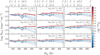 |
Fig. 6. H2O line fluxes as a function of the energy of the upper levels obtained from our MOLPOP-CEP runs. Here we report output predictions for different values of water vapor column density (from left to rightNH2O = 1017, 1018, 1018.5 cm−2) and continuum optical depth (from top to bottomτ100 = 0.1, 1.0, 10) as reported at the upper right corner of each panel. The H2O fluxes in each panel are color-coded according to the dust temperature (Tdust). |
Best-fit dust and gas properties of quasar host galaxies retrieved from H2O SLED modeling.
In general, our best-fit models aptly reproduce the observed H2O SLEDs in our quasar host galaxies. All the modeled H2O line luminosity ratios are consistent within the uncertainties with the measured data, except for a few line ratios. The worst case is that of J2310+1855 SLED fit, where the best-fit model underestimates the H2O 202 − 111- and 321 − 312-to-312 − 303 ratios – which, however, are consistent within ∼2σ with the observations. However, we note that deviations in ratios involving low-J lines may be expected if there is an additional low-excitation ISM component (see, e.g., González-Alfonso et al. 2010; Liu et al. 2017; Yang et al. 2020).
The posterior probability distributions of free parameters in Fig. 7 point to very high dust temperature ranging in Tdust ∼ 80 − 190 K with the highest values found in those sources in which the high-J H2O 422 − 413 line is detected. This fact is in accordance with our discussion given in Sect. 7.1. The best-fit models predict optically thin continuum conditions at 100 μm (i.e., τ100 < 1), except in the case of the J2310+1855 quasar for which τ100 ∼ 1 is favored within the uncertainties. The latter result is consistent within ∼1.5σ with what we found from the modeling of the dust SED at FIR wavelengths (τ100 ≈ 3.6). In the case of J1148+5251, the analysis of dust SED points to τ100 = 1.0 ± 0.4 which is still consistent within ∼2σ with the optically-thin regime suggested by the best-fit H2O SLED model. Conversely, the dust SED modeling of J0439+1634 suggests instead optically thick conditions. However, the latter is affected by large uncertainties. Finally, high H2O column density NH2O ∼ 2 × 10¹⁷ − 3 × 1018 cm−2 is needed in order to match the observations. Assuming our fiducial values of H2O abundance (XH2O = 2 × 10⁻⁶) and gas density (nH2 = 104.5 cm−3), the best-fit H2O column densities translate to molecular hydrogen column densities of NH2 ∼ 1 × 10²³ − 2 × 1024 cm−2, which correspond to typical molecular cloud dimensions of R = NH2/nH2 ∼ 1 − 20 pc. This sanity check suggests that our model results are reasonable2. However, the best-fit results are affected by large uncertainties reflecting the spread of the parameter distributions in Fig. 7. The most precise predictions are obtained for J0439+1634, which is not surprising given the achieved high signal-to-noise ratios (S/N) of these observations.
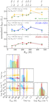 |
Fig. 7. Modeling of H2O SLEDs of quasar host galaxies. Top panels: colored diamonds are the observed H2O line luminosities normalized to the H2O 312 − 303 line as a function of the energy of the upper level (Eup). The green filled circles are the best-fit models obtained by using our MOLPOP-CEP grids. The best-fit parameters are reported at the top-left corner of each panel. The reported uncertainties take into account only statistical errors ignoring any systematics. Both the Eup and the normalized LH2O are reported in linear scale. Bottom panels: MCMC output posterior probability distributions of free parameters. The contour plots show 1-σ and 2σ confidence intervals. The same intervals are reported in the marginalized distributions. |
Our simple analysis reveals the presence of an intense warm dust component that can be responsible for the water vapor excitation in molecular clumps with high column density. In particular, for the quasar J2310+1855, we estimated a dust temperature of the optically-thick warm component of Tdust ∼ 150 K, which yields a blackbody SED peak at around rest-frame ≈20 μm. Remarkably, this value resembles the wavelength peak of the dusty torus component found by Shao et al. (2019), who performed a dust SED decomposition of J2310+1855 continuum emission over a wide wavelength range. This result could indicate a significant MIR contribution of the dusty torus in triggering the water vapor emission, at least in the quasar nuclear region. However, we cannot reach a similar conclusion for the quasar J1148+5251 when comparing the best-fit dust radiation field temperature with the dusty-torus component inferred by Leipski et al. (2013, 2014). For this source, our radiative transfer analysis predicts a dust temperature that is consistent within the uncertainties with that derived from dust SED modeling. Finally, we estimate a high dust temperature of Tdust ∼ 180 K in J0439+1634, suggesting the presence of a hot dust component in this quasar. Interestingly, Carniani et al. (2019), Yue et al. (2021), Walter et al. (2009), and Meyer et al. (2022) performed modeling of high-angular resolution ALMA/NOEMA observations of J2310+1855, J0439+1634, and J1148+5251, determining a FIR continuum half-light radius of ≈0.66 kpc, ≈0.74 kpc, and ≈1.9 kpc, respectively. This highlights that at least 50% of the dust mass is contained in a compact central region, especially in the case of J2310+1855, thus further supporting a significant contribution of compact warm or hot dust component in heating the molecular gas in this quasar host galaxy. In any case, with the current analysis and data, it is not possible to infer the geometrical properties (e.g., extension) of the bulk of the hot and warm dust components and the warm line-emitting region. Future high-angular resolution MIR/FIR studies will possibly reveal if the warm dust component we found could be actually associated to a central dusty torus in high-z quasars. Overall, our results are in line with similar analysis conducted in other sources at low- and high-z (e.g., González-Alfonso et al. 2010; van der Werf et al. 2011; Liu et al. 2017; Jarugula et al. 2019; Yang et al. 2020; Walter et al. 2022), predicting hot or warm dust components in the core regions of quasars, ULIRGs, SMGs, and normal star-forming galaxies, notwithstanding the different modeling details.
In order to find a constraint on the fraction of warm or hot dust component in our quasar host galaxies, we computed the expected observed flux density via Eq. (3), using the best-fit parameters obtained from MOLPOP-CEP. In the case of J2310+1855, and J1148+5251, we scaled Mdust in order to match the Herschel/PACS (Photodetector Array Camera Spectrometer; Poglitsch et al. 2010) data at (observed-frame) 100 μm (Leipski et al. 2014; Shao et al. 2019), while in the case of J0439+1634 we scaled the graybody model to match the JCMT/SCUBA-2 (James Clerk Maxwell Telescope/Submillimetre Common-User Bolometer Array-2; Holland et al. 2013) 666 GHz (observed-frame) upper limit (Yang et al. 2019a). As a result, we found that the fraction of warm or hot dust in our quasar host galaxies is ≲5 − 10% of the dust mass obtained from the dust FIR SED modeling. This result is in line with recent theoretical predictions on dust content in z ∼ 6 galaxies (Di Mascia et al. 2021).
7.3. Boltzmann diagrams of H2O levels
We note that the H2O SLED, despite being a powerful diagnostic tool, remains quite elusive for a intuitive understanding of the ISM excitation conditions without a detailed investigation of the various line ratios. This is mainly due to the interplay of collisions and radiative pumping mechanisms in exciting the water vapor lines. An analysis of the level population is required to better understand the H2O excitation by varying the gas and dust radiation field properties. The Boltzmann statistics predict that in local thermodynamical equilibrium (LTE) conditions the level population of a specie obeys to ni/ntot = gi/Q(T)exp(−Ei/kBT), where ni is density of the i-th level at energy Ei, gi is its quantum degeneracy, ntot is the total density of the species, and Q(T) is the partition function. Therefore, a thermalized level population is represented by a straight line in a ln(ni/gi)−Ei/kB diagram, the intercept and slope of which are determined by ntot/Q(T), and −1/T, respectively. Collisional excitation is expected to drive the level population of low H2O energy levels (E < 100 K) toward a Boltzmann distribution with an excitation temperature (Tex) near the gas kinetic temperature (Tkin), while the absorption of IR photons populates the high-energy level, such that Tex ∼ Tdust as soon as Tdust > Tkin. As a result of the interplay between collisional and radiative excitation, the H2O level population can be approximated by a double Tex: one value for the low-J lines (with Tex ∼ Tkin) and one for the higher-J lines (with Tex ∼ Tdust).
In Fig. 8, we show the level population diagrams for our three quasars as predicted by MOLPOP-CEP. These represent the volume densities of the level (weighted with their quantum degeneracy) at the H2O column density, continuum optical depth, and dust temperature obtained via the H2O SLED modeling discussed in the previous sections. In Fig. 8 we show a comparison of the population of the H2O levels in our quasars. The results show a significant contribution of the dust radiation field in exciting the high-J H2O lines in J2310+1855 compared to the other quasars. This is in line with the prominent peak of the H2O SLED in the 321 − 312 transition, and the mere detection of the H2O 422 − 413 line in the latter source. Indeed, significantly higher Tdust and τ100 values are inferred for this source. On the contrary, J1148+5251 appears much less excited in the high energy H2O levels consistently with the lack of H2O 422 − 413 line emission and the detection of the ground state line 111 − 000 indicating a minor contribution of the radiative pumping as a level populating mechanism. Finally, as also pointed out from the qualitative analysis in Sect. 7.1, J0439+1634 represents an intermediate case between J1148+5251 and J2310+1855.
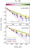 |
Fig. 8. Models of H2O population level diagrams (upper and lower panel, respectively, for ortho- and para-H2O) for our three quasar host galaxies. Each of the model shows the level volume density (weighted with their quantum degeneracy) at the NH2O, τ100, and Tdust values corresponding to the MOLPOP-CEP best-fit H2O SLED models (see Sect. 7.2). The straight lines are the analytical population diagrams computed assuming Boltzmann distribution color-coded by the excitation temperature. The green line corresponds to the LTE case (Tkin = Tex). |
7.4. LH2O − LTIR correlations
Previous studies have revealed the existence of nearly linear correlations between the luminosity of H2O lines (LH2O) and the total infrared luminosity (LTIR) extending over ∼12 orders of magnitude from young stellar objects (YSOs, San José-García 2015; San José-García et al. 2016), where H2O molecules are collisionally excited in shocked gas (e.g., Mottram et al. 2014), to high-z galaxies (Omont et al. 2013; Yang et al. 2013, 2016; Liu et al. 2017), in which radiative pumping plays an important role in populating the high-J H2O levels. However, these correlations have been interpreted differently in the Galactic and extragalactic context. In protostellar environments the H2O emission is spatially compact and located either in the very proximity of the protostars or in their molecular outflows that happens in the earliest stages of star formation. Here, the FIR luminosity traces the material in which the stars are forming in the protostellar envelopes but it has no direct effect on the water vapor excitation (see, e.g., van Dishoeck et al. 2021). On the other hand, in the extragalactic context the LH2O − LTIR correlations are thought to be the direct consequence of the IR pumping. In this sense, the water vapor emission arises in molecular clouds that are not necessarily co-spatial with the star-formation activity. However, recent studies (see, e.g., van Dishoeck et al. 2021, and references therein) showed that low- and mid-J H2O (Eup < 300 K) line ratios do not significantly differ in Galactic and extragalactic environments. This suggests a common mechanism for water vapor excitation extending from individual Galactic YSOs to high-z sources; namely, the H2O emission is likely a good tracer of star formation activity buried in the protostellar envelopes. Therefore, H2O traces proportionally the SFR as in the case of other dense gas tracers (e.g., HCN, Gao & Solomon 2004a,b). In particular, if a large fraction of the mass of the warm molecular ISM, where the bulk of the H2O emission arises, is spatially-correlated with the physical regions where most of the FIR is generated, the nature of the LH2O − LTIR correlations could be easily explained as driven by the size of the emitting region (see, e.g., González-Alfonso et al. 2014; Liu et al. 2017). Indeed, similar linear correlations are found for CO transitions which are collisionally excited in the molecular gas (see, e.g., Greve et al. 2014; Lu et al. 2014; Liu et al. 2015; Kamenetzky et al. 2016; Yang et al. 2017). These linear correlations reflect the well-established fact that star-formation (traced by LTIR) occurs within the molecular ISM (which mass is traced by the CO line emission). On the other hand, if the radiative pumping drives the excitation of H2O emission in high-z galaxies, then we might expect that this affects to some extent the LH2O − LTIR relation.
González-Alfonso et al. (2014) showed that steeper than linear LH2O − LTIR relation is expected if (on average) τ100 is an increasing function of LTIR. By using FIR pumping models, they predict a  for the H2O 202 − 111 line and similar supralinear relations for the other H2O transitions. However, Liu et al. (2017) showed that collisions significantly contribute to the excitation of the mid-J H2O lines, thus suggesting that the correlations are not the mere consequence of the radiative pumping effect. However, all the aforementioned investigations seem to suggest that LH2O − LTIR correlations are expected to be a consequence of either collisional excitation or IR pumping of H2O transitions. The lack of a clear correlation between H2O and TIR luminosities would suggest that a larger-than-expected variety in the ISM properties (gas density, temperature, geometry, chemical composition, etc.) is in place in the emitting regions.
In Fig. 9, we report the LH2O − LTIR correlations and the LH2O-to-LTIR ratios for the available lines in our quasar host galaxies. In order to study the correlations, we complement our data with previous observations from the literature. In particular, we retrieved measurements of local and high-z Hy/ULIRGs samples (Omont et al. 2013; Yang et al. 2013, 2016). We also included additional individual measurements of the quasar host galaxies APM 08279 at z = 3.9 (van der Werf et al. 2011), and PJ231-20 (PSO J231.6576-20.8335) at z = 6.59 (Pensabene et al. 2021); the Hy/ULIRGs/SMGs HLSJ0918 (HLSJ091828.6+514223, Combes et al. 2012; Rawle et al. 2014) at z = 5.2, and HFLS 3 at z = 6.34 (Riechers et al. 2013); the dusty star-forming galaxies (DSFGs) SPT 0538-50 at z = 2.78 (SPT-S J053816-5030.8, Bothwell et al. 2013), MAMBO-9 at z = 5.85 (MM J100026.36+021527.9, Casey et al. 2019), SPT 0346-52 at z = 5.66 (SPT-S J034640-5204.9, Apostolovski et al. 2019), and SPT 0311-58 at z = 6.9 (SPT-S J031132-5823.4, Jarugula et al. 2021); and the hot dust-obscured galaxy (Hot DOG) W0410-0913 (Stanley et al. 2021, with LTIR taken from Fan et al. 2016). When possible, we report the values corrected for gravitational lensing. In Fig. 9, we show that our data provide new constraints to the H2O − TIR luminosity relations at LTIR ≳ 1013 L⊙, and LH2O ≳ 108 L⊙, where only sparse detections are available in the literature thus far.
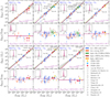 |
Fig. 9. Correlations between H2O line luminosities and total IR luminosities. The reference transition is reported in the upper left corner in the upper panels. Lower panels: report the correspondent LH2O/LTIR as a function of LTIR. Data points show measurements of local and high-z Hy/ULIRGs, SMGs, DSFGs/Hot DOGs, and QSO hosts retrieved from the literature, color-coded by their type. Different symbols indicate the literature references according to the legend. For the lensed quasar J0439+1634 we report the 95% confidence interval (red diamonds connected by a line) of intrinsic luminosities by adopting the magnification factor reported in Yang et al. (2019a, see also Sect.4). We use the mean magnification factor as the fiducial value in the fit. Data points with empty symbols are not corrected for gravitational lensing and were excluded from the fit. We also excluded those data reported with dotted error bars as explained in the text. Downward arrows are 3σ upper limits that we also ignored in the fit. The solid purple lines show our best-fit models. The inset panels show the posterior probability distribution of the slope α of the LH2O − LTIR correlations and β for LH2O/LTIR. The best-fit values are reported at the bottom right corner of each panel. For comparison we also show results obtained assuming an exact linear relation (dot-dashed green lines) and the best-fit models, from Yang et al. (2013, as dashed black lines). The shaded areas are 1-σ confidence intervals. References. van der Werf+11 (van der Werf et al. 2011), Combes+12 (Combes et al. 2012), Bothwell+13 (Bothwell et al. 2013), Omont+13 (Omont et al. 2013), Riechers+13 (Riechers et al. 2013), Yang+13,+16 (Yang et al. 2013, 2016), Rawle+14 (Rawle et al. 2014), Apostolovski+19 (Apostolovski et al. 2019), Casey+19 (Casey et al. 2019), Jarugula+21 (Jarugula et al. 2021), Pensabene+21 (Pensabene et al. 2021), Stanley+21 (Stanley et al. 2021). |
By assuming linear functional form of the type Log LH2O = α Log LTIR + β, we performed linear regressions in log-log space through a hierarchical Bayesian approach using the linmix Python package (Kelly 2007). In order to reduce possible biases in the fitting results, following Yang et al. (2013, 2016) we excluded M82 due to its peculiar very low values of its H2O lines (see Weiß et al. 2010; Yang et al. 2013, for a discussion); we then excluded SDP 81 due to missing flux filtered out by interferometer (Omont et al. 2013), and the H2O 321 − 312 transition of HFLS 3 due to its high LH2O-to-LTIR ratio. Finally, we excluded all the sources not corrected for gravitational magnification and all upper limit measurements on H2O luminosity. In the case of the lensed quasar J0439+1634, we derived the intrinsic luminosities by adopting a mean magnification factor of 4.6 (see Sect. 4, Yang et al. 2019a; Yue et al. 2021) and we used them as fiducial values in the fit. Finally, we also fit the LH2O/LTIR ratios by adopting the same aforementioned assumptions. Our best-fit results are reported in Fig. 9, and Table 6. For comparison, we report the relation found by (Yang et al. 2013) and the best-fit models obtained assuming an exact linear relation (i.e., α = 1).
Best-fit slopes of LH2O − LTIR relations and averaged LH2O/LTIR ratios.
Overall, our best-fit slopes suggest slightly supralinear relations in all the cases except for the ground base transition H2O 111 − 000 that is consistent with a linear relation within the uncertainty. A similar result is valid in the case of H2O 422 − 413 line which relation is also roughly linear within ∼1-σ. However, the relations involving the H2O 111 − 000, and 422 − 413 lines are constrained using a low number of data points available in the literature. This is reflected in the larger relative error on the correlation slopes with respect to the other lines. The slopes of the correlations are all consistent within the uncertainties with those found by Yang et al. (2013, 2016). The supralinear trend of the LH2O − LTIR correlations support the idea that (at least for mid- and high-J H2O lines) the correlations are likely driven by the IR pumping effect rather than the mere co-spatiality of the line- and IR-continuum-emitting region (see González-Alfonso et al. 2014). The intrinsic scatter about the H2O − TIR relations are ∼0.2 dex (see Table 6), which is comparable or even lower with regard to that of the linear relation between CO lines and the FIR luminosity (see, e.g., Liu et al. 2015; Kamenetzky et al. 2016). Our analysis of the LH2O/LTIR ratios leads to similar average values than that reported by Yang et al. (2013, 2016). We do not find any substantial difference in the H2O-to-TIR luminosity ratios measured in our high-z quasars than those of local AGN and star-forming galaxies, which is expected if H2O is a pure tracer of the buried star-formation activity.
8. Summary and conclusions
We present NOEMA observations toward three IR-bright quasars (J2310+1855, J1148+5251, J0439+1634) at z > 6 that were targeted in multiple water vapor lines as well as in the FIR continuum. These quasars were previously detected in multiple ISM probes including some H2O lines. The lines targeted in the new observations are the para-/ortho-H2O 312 − 303, 111 − 000, 220 − 211, and 422 − 413 emission lines, with most being detected in all three quasars. The combination of our new and the previous H2O detections enable us to investigate the warm and dense phase of the ISM, and the local IR dust radiation field in intensely star-forming galaxies at cosmic dawn. We pose new constraints on the LH2O − LTIR relations which enclose key information on the H2O excitation mechanisms. In order to interpret our results and place quantitative constraints on the physical parameters of the ISM, we employed the MOLPOP-CEP radiative transfer code. The main results of this work are as follows:
-
We model the FIR dust continuum emission in all quasar host galaxies by assuming a single-component modified blackbody and taking into account the effect of the dust optical depth and the CMB contrast. With this approach, we infer the dust masses, temperatures, continuum optical depths, IR luminosities, and SFRs for the three quasar host galaxies (see Sect. 5 and Table 4). Our results suggest Tdust ∼ 80 − 90 K, which is higher than the values previously reported in the literature, assuming optically thin dust emission.
-
Our H2O SLEDs do not show any obvious imprinting of powerful AGN activity characterizing our sources when compared to the SLEDs of local ULIRGs, AGN, as well as other high-z sources. However, on the basis of the H2O excitation physics, a detailed qualitative analysis of the individual line ratios suggests that the bulk of H2O emission in J1148+5251 arises from warm ISM phase with a low continuum opacity. A similar analysis point to the presence of relatively warmer dust in J2310+1855, and J0439+1634 that boosts the excitation of high-J H2O lines compared to J1148+5251.
-
Using MOLPOP-CEP predictions, we modeled the observed H2O SLEDs of the quasar host galaxies. Our results reproduce the observed data well. The best-fit models reveal the presence of a warm dust component the temperature of which ranges in Tdust ∼ 80 − 190 K. Here, the highest temperatures are found in those sources that are detected in their high-lying J = 4 H2O transition. This warm dust component is presumably more compact than that probed by standard dust SED modeling. From our results we estimate that the mass fraction of the warm or hot dust component in our quasars host galaxies is ≲5 − 10%.
-
Our best-fit models point to water vapor column densities in the range NH2O ∼ 2 × 10¹⁷ − 3 × 1018 cm−2. Optically thin conditions (τ100 ≲ 1) for the continuum are predicted in all sources, except for J2310+1855 for which τ100 ∼ 1, consistent with the qualitative analysis of the H2O SLEDs. Interestingly, our radiative transfer analysis on the H2O SLED of J1148+5251, and J2310+1855 predicts values of τ100 which are consistent within ∼2σ with the results obtained from the dust SED modeling. We find a significantly higher contribution of IR pumping in populating the high-J H2O lines in J2310+1855 compared to the other quasars. The excitation temperatures of E > 200 K H2O levels are roughly Tex ∼ 40 − 50 K, while they are around Tex ∼ 25 − 30 K in J1148+5251.
-
We studied the correlations between H2O and TIR luminosities and the H2O-to-TIR luminosity ratios. Our observations, in combination with data from the literature, allow us to put constraints on the LTIR ≳ 1013 L⊙ and LH2O ≳ 108 L⊙ part of the correlations. Our results suggest supralinear trends in all the cases – except for the H2O 111 − 000 lines whose correlation with LTIR is aptly consistent with a linear trend, albeit poorly sampled. Overall, our results support the notion that (at least for mid- and high-J H2O transitions) the LH2O − LTIR correlations are driven by the radiation pumping of the lines rather than the co-spatiality of the H2O-line- and IR-continuum-emitting regions. The analysis of the LH2O/LTIR ratios does not highlight any significant difference between values measured in high-z and local AGN and that observed in local star-forming galaxies. Given the small intrinsic scatter of the H2O-TIR relations, this result suggests that H2O can be also used as a robust proxy of star formation in high-z quasar host galaxies.
We showed how the combination of multiple H2O lines enables us to shed light on the properties of the warm molecular medium in massive galaxies in the Epoch of Reionization. Water vapor lines are also powerful diagnostics of the warm dust component that is difficult to unveil through a simple analysis of the dust continuum SED. However, at z ∼ 6, many key H2O lines are shifted in ALMA/NOEMA (sub-)mm bands such that they can be simultaneously targeted. In particular, at z = 6, the combination of H2O 312 − 312, 312 − 221 (the latter of which is blended with the CO(10 − 9) line), or the H2O 312 − 303 together with the H2O 111 − 000, are encompassed in a < 3 GHz bandwidth and can be therefore secured with a single ALMA or NOEMA frequency setting. Despite the complexity of the water vapor excitation analysis that requires multiple H2O line detections, our work suggests that the aforementioned combinations of lines maximize the scientific return of H2O observations for the purpose of probing the warm and dense ISM in galaxies at z ≳ 6. Such observations will also provide relatively tight constraints on TIR luminosity (the H2O 321 − 303 − TIR shows small intrinsic scatter).
Our studies were limited by the low S/N of the current data. Further investigations on a larger sample of sources targeting multiple H2O lines with deeper observations are required in order to determine if our results are characteristic of the z > 6 quasar population. Overall, our analysis shows that the H2O lines do not seem to be significantly affected by the extreme BH feedback in z > 6 quasars when compared to water vapor emission in local star-forming galaxies. However, larger samples are required to further understand whether H2O lines can provide information on AGN activity or if they can be used as pure tracers of star formation in high-z quasar host galaxies. In addition, the brightness of H2O lines, compared to other typically used molecular tracers, makes them ideal probes of the shocked medium by AGN-driven outflows. Future deeper (sub-)mm spectroscopic observations of primeval quasar host galaxies would also enable the systematic search for H2O lines featuring P-Cygni profiles that are known to be a smoking gun of massive molecular outflows.
The code is available at the following link: https://github.com/aasensio/molpop-cep
We stress that these values have to be taken with caution since they depend on the model assumptions.
Acknowledgments
We thank the anonymous referee for a careful reading of the manuscript and for the useful comments and suggestions that greatly improved the paper. Based on observations carried out under project number S19DL with the IRAM NOEMA Interferometer. IRAM is supported by INSU/CNRS (France), MPG (Germany) and IGN (Spain). We acknowledge IRAM staff for help provided during the observations and for data reduction. AP acknowledges support from Fondazione Cariplo grant no. 2020-0902. RAM acknowledges support from the ERC Advanced Grant 740246 (Cosmic Gas). This research made use of Astropy(http://www.astropy.org), a community-developed core Python package for Astronomy (Astropy Collaboration 2013, 2018), NumPy (Harris et al. 2020), SciPy (Virtanen et al. 2020), and Matplotlib (Hunter 2007).
References
- Apostolovski, Y., Aravena, M., Anguita, T., et al. 2019, A&A, 628, A23 [NASA ADS] [CrossRef] [EDP Sciences] [Google Scholar]
- Asensio Ramos, A., & Elitzur, M. 2018, A&A, 616, A131 [NASA ADS] [CrossRef] [EDP Sciences] [Google Scholar]
- Astropy Collaboration (Robitaille, T. P., et al.) 2013, A&A, 558, A33 [NASA ADS] [CrossRef] [EDP Sciences] [Google Scholar]
- Astropy Collaboration (Price-Whelan, A. M., et al.) 2018, AJ, 156, 123 [Google Scholar]
- Beelen, A., Cox, P., Benford, D. J., et al. 2006, ApJ, 642, 694 [NASA ADS] [CrossRef] [Google Scholar]
- Behrens, C., Pallottini, A., Ferrara, A., Gallerani, S., & Vallini, L. 2018, MNRAS, 477, 552 [NASA ADS] [CrossRef] [Google Scholar]
- Bertoldi, F., Carilli, C. L., Cox, P., et al. 2003a, A&A, 406, L55 [NASA ADS] [CrossRef] [EDP Sciences] [Google Scholar]
- Bertoldi, F., Cox, P., Neri, R., et al. 2003b, A&A, 409, L47 [NASA ADS] [CrossRef] [EDP Sciences] [Google Scholar]
- Blain, A. W., Barnard, V. E., & Chapman, S. C. 2003, MNRAS, 338, 733 [Google Scholar]
- Bothwell, M. S., Aguirre, J. E., Chapman, S. C., et al. 2013, ApJ, 779, 67 [NASA ADS] [CrossRef] [Google Scholar]
- Bradford, C. M., Bolatto, A. D., Maloney, P. R., et al. 2011, ApJ, 741, L37 [Google Scholar]
- Carniani, S., Gallerani, S., Vallini, L., et al. 2019, MNRAS, 489, 3939 [NASA ADS] [Google Scholar]
- Casey, C. M. 2012, MNRAS, 425, 3094 [Google Scholar]
- Casey, C. M., Narayanan, D., & Cooray, A. 2014, Phys. Rep., 541, 45 [Google Scholar]
- Casey, C. M., Zavala, J. A., Aravena, M., et al. 2019, ApJ, 887, 55 [Google Scholar]
- Cicone, C., Maiolino, R., Gallerani, S., et al. 2015, A&A, 574, A14 [NASA ADS] [CrossRef] [EDP Sciences] [Google Scholar]
- Combes, F., & Wiklind, T. 1997, ApJ, 486, L79 [NASA ADS] [CrossRef] [Google Scholar]
- Combes, F., Rex, M., Rawle, T. D., et al. 2012, A&A, 538, L4 [NASA ADS] [CrossRef] [EDP Sciences] [Google Scholar]
- Conley, A., Cooray, A., Vieira, J. D., et al. 2011, ApJ, 732, L35 [NASA ADS] [CrossRef] [Google Scholar]
- da Cunha, E., Groves, B., Walter, F., et al. 2013, ApJ, 766, 13 [Google Scholar]
- Daniel, F., Dubernet, M. L., & Grosjean, A. 2011, A&A, 536, A76 [NASA ADS] [CrossRef] [EDP Sciences] [Google Scholar]
- De Rosa, G., Decarli, R., Walter, F., et al. 2011, ApJ, 739, 56 [NASA ADS] [CrossRef] [Google Scholar]
- De Rosa, G., Venemans, B. P., Decarli, R., et al. 2014, ApJ, 790, 145 [Google Scholar]
- Decarli, R., Walter, F., Venemans, B. P., et al. 2018, ApJ, 854, 97 [Google Scholar]
- Decarli, R., Dotti, M., Bañados, E., et al. 2019, ApJ, 880, 157 [Google Scholar]
- Di Mascia, F., Gallerani, S., Behrens, C., et al. 2021, MNRAS, 503, 2349 [NASA ADS] [CrossRef] [Google Scholar]
- Draine, B. T. 2003, ARA&A, 41, 241 [NASA ADS] [CrossRef] [Google Scholar]
- Draine, B. T., & Lee, H. M. 1984, ApJ, 285, 89 [NASA ADS] [CrossRef] [Google Scholar]
- Dunne, L., & Eales, S. A. 2001, MNRAS, 327, 697 [Google Scholar]
- Elitzur, M., & Asensio Ramos, A. 2006, MNRAS, 365, 779 [Google Scholar]
- Faisst, A. L., Fudamoto, Y., Oesch, P. A., et al. 2020, MNRAS, 498, 4192 [NASA ADS] [CrossRef] [Google Scholar]
- Fan, L., Han, Y., Nikutta, R., Drouart, G., & Knudsen, K. K. 2016, ApJ, 823, 107 [Google Scholar]
- Fan, X., Wang, F., Yang, J., et al. 2019, ApJ, 870, L11 [Google Scholar]
- Farrah, D., Afonso, J., Efstathiou, A., et al. 2003, MNRAS, 343, 585 [Google Scholar]
- Faure, A., Crimier, N., Ceccarelli, C., et al. 2007, A&A, 472, 1029 [NASA ADS] [CrossRef] [EDP Sciences] [Google Scholar]
- Feruglio, C., Fiore, F., Carniani, S., et al. 2018, A&A, 619, A39 [NASA ADS] [CrossRef] [EDP Sciences] [Google Scholar]
- Fischer, J., Luhman, M. L., Satyapal, S., et al. 1999, Ap&SS, 266, 91 [NASA ADS] [CrossRef] [Google Scholar]
- Fischer, J., Sturm, E., González-Alfonso, E., et al. 2010, A&A, 518, L41 [NASA ADS] [CrossRef] [EDP Sciences] [Google Scholar]
- Foreman-Mackey, D., Hogg, D. W., Lang, D., & Goodman, J. 2013, PASP, 125, 306 [Google Scholar]
- Galametz, M., Kennicutt, R. C., Albrecht, M., et al. 2012, MNRAS, 425, 763 [NASA ADS] [CrossRef] [Google Scholar]
- Gallerani, S., Ferrara, A., Neri, R., & Maiolino, R. 2014, MNRAS, 445, 2848 [Google Scholar]
- Gao, Y., & Solomon, P. M. 2004a, ApJS, 152, 63 [Google Scholar]
- Gao, Y., & Solomon, P. M. 2004b, ApJ, 606, 271 [NASA ADS] [CrossRef] [Google Scholar]
- Goicoechea, J. R., Martín-Pintado, J., & Cernicharo, J. 2005, ApJ, 619, 291 [NASA ADS] [CrossRef] [Google Scholar]
- González-Alfonso, E., Smith, H. A., Fischer, J., & Cernicharo, J. 2004, ApJ, 613, 247 [Google Scholar]
- González-Alfonso, E., Smith, H. A., Ashby, M. L. N., et al. 2008, ApJ, 675, 303 [CrossRef] [Google Scholar]
- González-Alfonso, E., Fischer, J., Isaak, K., et al. 2010, A&A, 518, L43 [NASA ADS] [CrossRef] [EDP Sciences] [Google Scholar]
- González-Alfonso, E., Fischer, J., Graciá-Carpio, J., et al. 2012, A&A, 541, A4 [NASA ADS] [CrossRef] [EDP Sciences] [Google Scholar]
- González-Alfonso, E., Fischer, J., Bruderer, S., et al. 2013, A&A, 550, A25 [NASA ADS] [CrossRef] [EDP Sciences] [Google Scholar]
- González-Alfonso, E., Fischer, J., Aalto, S., & Falstad, N. 2014, A&A, 567, A91 [NASA ADS] [CrossRef] [EDP Sciences] [Google Scholar]
- Greve, T. R., Leonidaki, I., Xilouris, E. M., et al. 2014, ApJ, 794, 142 [NASA ADS] [CrossRef] [Google Scholar]
- Harrington, K. C., Weiss, A., Yun, M. S., et al. 2021, ApJ, 908, 95 [NASA ADS] [CrossRef] [Google Scholar]
- Harris, C. R., Millman, K. J., van der Walt, S. J., et al. 2020, Nature, 585, 357 [NASA ADS] [CrossRef] [Google Scholar]
- Hashimoto, T., Inoue, A. K., Tamura, Y., et al. 2019, PASJ, 71, 109 [NASA ADS] [CrossRef] [Google Scholar]
- Helou, G., Soifer, B. T., & Rowan-Robinson, M. 1985, ApJ, 298, L7 [Google Scholar]
- Helou, G., Khan, I. R., Malek, L., & Boehmer, L. 1988, ApJS, 68, 151 [NASA ADS] [CrossRef] [Google Scholar]
- Herrera-Camus, R., Sturm, E., Graciá-Carpio, J., et al. 2020, A&A, 633, L4 [Google Scholar]
- Holland, W. S., Bintley, D., Chapin, E. L., et al. 2013, MNRAS, 430, 2513 [Google Scholar]
- Hunter, J. D. 2007, Comput. Sci. Eng., 9, 90 [NASA ADS] [CrossRef] [Google Scholar]
- Imanishi, M., Hagiwara, Y., Horiuchi, S., Izumi, T., & Nakanishi, K. 2021, MNRAS, 502, L79 [NASA ADS] [CrossRef] [Google Scholar]
- Jarugula, S., Vieira, J. D., Spilker, J. S., et al. 2019, ApJ, 880, 92 [Google Scholar]
- Jarugula, S., Vieira, J. D., Weiss, A., et al. 2021, ApJ, 921, 97 [NASA ADS] [CrossRef] [Google Scholar]
- Jiang, L., Fan, X., Vestergaard, M., et al. 2007, AJ, 134, 1150 [NASA ADS] [CrossRef] [Google Scholar]
- Jones, G. C., Carilli, C. L., Shao, Y., et al. 2017, ApJ, 850, 180 [Google Scholar]
- Kamenetzky, J., Glenn, J., Rangwala, N., et al. 2012, ApJ, 753, 70 [Google Scholar]
- Kamenetzky, J., Rangwala, N., Glenn, J., Maloney, P. R., & Conley, A. 2016, ApJ, 829, 93 [Google Scholar]
- Kelly, B. C. 2007, ApJ, 665, 1489 [Google Scholar]
- Kessler, M. F., Steinz, J. A., Anderegg, M. E., et al. 1996, A&A, 500, 493 [Google Scholar]
- Kirkpatrick, A., Pope, A., Alexander, D. M., et al. 2012, ApJ, 759, 139 [Google Scholar]
- Kirkpatrick, A., Pope, A., Sajina, A., et al. 2015, ApJ, 814, 9 [NASA ADS] [CrossRef] [Google Scholar]
- Koptelova, E., & Hwang, C.-Y. 2019, ApJ, 880, L19 [NASA ADS] [CrossRef] [Google Scholar]
- Kroupa, P. 2001, MNRAS, 322, 231 [NASA ADS] [CrossRef] [Google Scholar]
- Lehnert, M. D., Yang, C., Emonts, B. H. C., et al. 2020, A&A, 641, A124 [NASA ADS] [CrossRef] [EDP Sciences] [Google Scholar]
- Leipski, C., Meisenheimer, K., Walter, F., et al. 2013, ApJ, 772, 103 [NASA ADS] [CrossRef] [Google Scholar]
- Leipski, C., Meisenheimer, K., Walter, F., et al. 2014, ApJ, 785, 154 [Google Scholar]
- Li, J., Wang, R., Cox, P., et al. 2020a, ApJ, 900, 131 [NASA ADS] [CrossRef] [Google Scholar]
- Li, J., Wang, R., Riechers, D., et al. 2020b, ApJ, 889, 162 [NASA ADS] [CrossRef] [Google Scholar]
- Liang, L., Feldmann, R., Kereš, D., et al. 2019, MNRAS, 489, 1397 [NASA ADS] [CrossRef] [Google Scholar]
- Lis, D. C., Neufeld, D. A., Phillips, T. G., Gerin, M., & Neri, R. 2011, ApJ, 738, L6 [Google Scholar]
- Liu, D., Gao, Y., Isaak, K., et al. 2015, ApJ, 810, L14 [NASA ADS] [CrossRef] [Google Scholar]
- Liu, L., Weiß, A., Perez-Beaupuits, J. P., et al. 2017, ApJ, 846, 5 [Google Scholar]
- Lu, N., Zhao, Y., Xu, C. K., et al. 2014, ApJ, 787, L23 [Google Scholar]
- Lupu, R. E., Scott, K. S., Aguirre, J. E., et al. 2012, ApJ, 757, 135 [Google Scholar]
- Maiolino, R., Cox, P., Caselli, P., et al. 2005, A&A, 440, L51 [NASA ADS] [CrossRef] [EDP Sciences] [Google Scholar]
- Maiolino, R., Gallerani, S., Neri, R., et al. 2012, MNRAS, 425, L66 [Google Scholar]
- Mazzucchelli, C., Bañados, E., Venemans, B. P., et al. 2017, ApJ, 849, 91 [Google Scholar]
- Meijerink, R., & Spaans, M. 2005, A&A, 436, 397 [CrossRef] [EDP Sciences] [Google Scholar]
- Meijerink, R., Kristensen, L. E., Weiß, A., et al. 2013, ApJ, 762, L16 [Google Scholar]
- Menten, K. M., Lundgren, A., Belloche, A., Thorwirth, S., & Reid, M. J. 2008, A&A, 477, 185 [NASA ADS] [CrossRef] [EDP Sciences] [Google Scholar]
- Meyer, R. A., Walter, F., Cicone, C., et al. 2022, ApJ, 927, 152 [NASA ADS] [CrossRef] [Google Scholar]
- Mottram, J. C., Kristensen, L. E., van Dishoeck, E. F., et al. 2014, A&A, 572, A21 [NASA ADS] [CrossRef] [EDP Sciences] [Google Scholar]
- Murphy, E. J., Condon, J. J., Schinnerer, E., et al. 2011, ApJ, 737, 67 [Google Scholar]
- Neeleman, M., Bañados, E., Walter, F., et al. 2019, ApJ, 882, 10 [Google Scholar]
- Neeleman, M., Novak, M., Venemans, B. P., et al. 2021, ApJ, 911, 141 [NASA ADS] [CrossRef] [Google Scholar]
- Novak, M., Bañados, E., Decarli, R., et al. 2019, ApJ, 881, 63 [NASA ADS] [CrossRef] [Google Scholar]
- Omont, A., Neri, R., Cox, P., et al. 2011, A&A, 530, L3 [NASA ADS] [CrossRef] [EDP Sciences] [Google Scholar]
- Omont, A., Yang, C., Cox, P., et al. 2013, A&A, 551, A115 [NASA ADS] [CrossRef] [EDP Sciences] [Google Scholar]
- Pensabene, A., Carniani, S., Perna, M., et al. 2020, A&A, 637, A84 [NASA ADS] [CrossRef] [EDP Sciences] [Google Scholar]
- Pensabene, A., Decarli, R., Bañados, E., et al. 2021, A&A, 652, A66 [NASA ADS] [CrossRef] [EDP Sciences] [Google Scholar]
- Pereira-Santaella, M., Spinoglio, L., Busquet, G., et al. 2013, ApJ, 768, 55 [Google Scholar]
- Pickett, H. M., Poynter, R. L., Cohen, E. A., et al. 1998, J. Quant. Spectr. Rad. Transf., 60, 883 [Google Scholar]
- Pilbratt, G. L., Riedinger, J. R., Passvogel, T., et al. 2010, A&A, 518, L1 [NASA ADS] [CrossRef] [EDP Sciences] [Google Scholar]
- Planck Collaboration XIII. 2016, A&A, 594, A13 [NASA ADS] [CrossRef] [EDP Sciences] [Google Scholar]
- Poelman, D. R., Spaans, M., & Tielens, A. G. G. M. 2007, A&A, 464, 1023 [NASA ADS] [CrossRef] [EDP Sciences] [Google Scholar]
- Poglitsch, A., Waelkens, C., Geis, N., et al. 2010, A&A, 518, L2 [NASA ADS] [CrossRef] [EDP Sciences] [Google Scholar]
- Rangwala, N., Maloney, P. R., Glenn, J., et al. 2011, ApJ, 743, 94 [NASA ADS] [CrossRef] [Google Scholar]
- Rawle, T. D., Egami, E., Bussmann, R. S., et al. 2014, ApJ, 783, 59 [NASA ADS] [CrossRef] [Google Scholar]
- Riechers, D. A., Walter, F., Bertoldi, F., et al. 2009, ApJ, 703, 1338 [NASA ADS] [CrossRef] [Google Scholar]
- Riechers, D. A., Bradford, C. M., Clements, D. L., et al. 2013, Nature, 496, 329 [Google Scholar]
- Riechers, D. A., Leung, T. K. D., Ivison, R. J., et al. 2017, ApJ, 850, 1 [Google Scholar]
- Riechers, D. A., Nayyeri, H., Burgarella, D., et al. 2021, ApJ, 907, 62 [NASA ADS] [CrossRef] [Google Scholar]
- Riechers, D. A., Weiss, A., Walter, F., et al. 2022, Nature, 602, 58 [NASA ADS] [CrossRef] [Google Scholar]
- Rivera, J., Baker, A. J., Gallardo, P. A., et al. 2019, ApJ, 879, 95 [NASA ADS] [CrossRef] [Google Scholar]
- Robson, I., Priddey, R. S., Isaak, K. G., & McMahon, R. G. 2004, MNRAS, 351, L29 [NASA ADS] [CrossRef] [Google Scholar]
- San José-García, I. 2015, Ph.D. Thesis, Leiden University, The Netherlands [Google Scholar]
- San José-García, I., Mottram, J. C., van Dishoeck, E. F., et al. 2016, A&A, 585, A103 [CrossRef] [EDP Sciences] [Google Scholar]
- Sanders, D. B., Mazzarella, J. M., Kim, D. C., Surace, J. A., & Soifer, B. T. 2003, AJ, 126, 1607 [Google Scholar]
- Schindler, J.-T., Farina, E. P., Bañados, E., et al. 2020, ApJ, 905, 51 [Google Scholar]
- Scoville, N., Sheth, K., Aussel, H., et al. 2016, ApJ, 820, 83 [Google Scholar]
- Shao, Y., Wang, R., Jones, G. C., et al. 2017, ApJ, 845, 138 [NASA ADS] [CrossRef] [Google Scholar]
- Shao, Y., Wang, R., Carilli, C. L., et al. 2019, ApJ, 876, 99 [NASA ADS] [CrossRef] [Google Scholar]
- Simpson, J. M., Smail, I., Swinbank, A. M., et al. 2017, ApJ, 839, 58 [NASA ADS] [CrossRef] [Google Scholar]
- Solomon, P. M., Downes, D., Radford, S. J. E., & Barrett, J. W. 1997, ApJ, 478, 144 [NASA ADS] [CrossRef] [Google Scholar]
- Sommovigo, L., Ferrara, A., Carniani, S., et al. 2021, MNRAS, 503, 4878 [NASA ADS] [CrossRef] [Google Scholar]
- Spinoglio, L., Pereira-Santaella, M., Busquet, G., et al. 2012, ApJ, 758, 108 [Google Scholar]
- Stanley, F., Knudsen, K. K., Aalto, S., et al. 2021, A&A, 646, A178 [NASA ADS] [CrossRef] [EDP Sciences] [Google Scholar]
- Sturm, E., González-Alfonso, E., Veilleux, S., et al. 2011, ApJ, 733, L16 [NASA ADS] [CrossRef] [Google Scholar]
- Tripodi, R., Feruglio, C., Fiore, F., et al. 2022, A&A, 665, A107 [NASA ADS] [CrossRef] [EDP Sciences] [Google Scholar]
- van der Tak, F. F. S., Weiß, A., Liu, L., & Güsten, R. 2016, A&A, 593, A43 [NASA ADS] [CrossRef] [EDP Sciences] [Google Scholar]
- van der Werf, P. P., Isaak, K. G., Meijerink, R., et al. 2010, A&A, 518, L42 [NASA ADS] [CrossRef] [EDP Sciences] [Google Scholar]
- van der Werf, P. P., Berciano Alba, A., Spaans, M., et al. 2011, ApJ, 741, L38 [Google Scholar]
- van Dishoeck, E. F., Kristensen, L. E., Mottram, J. C., et al. 2021, A&A, 648, A24 [NASA ADS] [CrossRef] [EDP Sciences] [Google Scholar]
- Venemans, B. P., Walter, F., Decarli, R., et al. 2017a, ApJ, 837, 146 [NASA ADS] [CrossRef] [Google Scholar]
- Venemans, B. P., Walter, F., Decarli, R., et al. 2017b, ApJ, 845, 154 [Google Scholar]
- Venemans, B. P., Decarli, R., Walter, F., et al. 2018, ApJ, 866, 159 [Google Scholar]
- Venemans, B. P., Neeleman, M., Walter, F., et al. 2019, ApJ, 874, L30 [NASA ADS] [CrossRef] [Google Scholar]
- Venemans, B. P., Walter, F., Neeleman, M., et al. 2020, ApJ, 904, 130 [Google Scholar]
- Virtanen, P., Gommers, R., Oliphant, T. E., et al. 2020, Nat. Methods, 17, 261 [Google Scholar]
- Walter, F. 2009, in Cosmic Dust - Near and Far, eds. T. Henning, E. Grün, & J. Steinacker, ASP Conf. Ser., 414, 287 [NASA ADS] [Google Scholar]
- Walter, F., Bertoldi, F., Carilli, C., et al. 2003, Nature, 424, 406 [Google Scholar]
- Walter, F., Carilli, C., Bertoldi, F., et al. 2004, ApJ, 615, L17 [NASA ADS] [CrossRef] [Google Scholar]
- Walter, F., Riechers, D., Cox, P., et al. 2009, Nature, 457, 699 [NASA ADS] [CrossRef] [Google Scholar]
- Walter, F., Riechers, D., Novak, M., et al. 2018, ApJ, 869, L22 [NASA ADS] [CrossRef] [Google Scholar]
- Walter, F., Neeleman, M., Decarli, R., et al. 2022, ApJ, 927, 21 [NASA ADS] [CrossRef] [Google Scholar]
- Wang, F., Wang, R., Fan, X., et al. 2019, ApJ, 880, 2 [NASA ADS] [CrossRef] [Google Scholar]
- Wang, R., Carilli, C. L., Beelen, A., et al. 2007, AJ, 134, 617 [NASA ADS] [CrossRef] [Google Scholar]
- Wang, R., Wagg, J., Carilli, C. L., et al. 2008, AJ, 135, 1201 [NASA ADS] [CrossRef] [Google Scholar]
- Wang, R., Wagg, J., Carilli, C. L., et al. 2011, AJ, 142, 101 [NASA ADS] [CrossRef] [Google Scholar]
- Wang, R., Wagg, J., Carilli, C. L., et al. 2013, ApJ, 773, 44 [Google Scholar]
- Weiß, A., Requena-Torres, M. A., Güsten, R., et al. 2010, A&A, 521, L1 [NASA ADS] [CrossRef] [EDP Sciences] [Google Scholar]
- Yang, C., Gao, Y., Omont, A., et al. 2013, ApJ, 771, L24 [NASA ADS] [CrossRef] [Google Scholar]
- Yang, C., Omont, A., Beelen, A., et al. 2016, A&A, 595, A80 [NASA ADS] [CrossRef] [EDP Sciences] [Google Scholar]
- Yang, C., Omont, A., Beelen, A., et al. 2017, A&A, 608, A144 [NASA ADS] [CrossRef] [EDP Sciences] [Google Scholar]
- Yang, C., Gavazzi, R., Beelen, A., et al. 2019b, A&A, 624, A138 [NASA ADS] [CrossRef] [EDP Sciences] [Google Scholar]
- Yang, C., González-Alfonso, E., Omont, A., et al. 2020, A&A, 634, L3 [NASA ADS] [CrossRef] [EDP Sciences] [Google Scholar]
- Yang, J., Venemans, B., Wang, F., et al. 2019a, ApJ, 880, 153 [NASA ADS] [CrossRef] [Google Scholar]
- Yang, J., Wang, F., Fan, X., et al. 2021, ApJ, 923, 262 [NASA ADS] [CrossRef] [Google Scholar]
- Yue, M., Yang, J., Fan, X., et al. 2021, ApJ, 917, 99 [NASA ADS] [CrossRef] [Google Scholar]
- Zhang, Z.-Y., Papadopoulos, P. P., Ivison, R. J., et al. 2016, R. Soc. Open Sci., 3 [Google Scholar]
All Tables
Best-fit dust and gas properties of quasar host galaxies retrieved from H2O SLED modeling.
All Figures
|
Fig. 1. Energy level diagram of H2O. Downward solid red and gray arrows are the transitions reported in this paper and those available in the literature (see Yang et al. 2019a, Li et al. 2020b, Riechers et al., in prep.). The upward dashed orange arrows indicate the FIR H2O pumping (absorption) lines of interest. The respective wavelengths are also reported. |
| In the text | |
|
Fig. 2. NOEMA spectra of the three z > 6 quasars J2310+1855, J1148+5251 and J0439+1634 (from top to bottom). We report the observed data in light blue and the best-fit models in red. The blue dashed lines indicate the rest frequencies of the targeted H2O transitions (quantum numbers are also reported). At the bottom of each spectra, we report the residuals (data-model). The gray-shaded areas show the noise RMS across the spectra. |
| In the text | |
|
Fig. 3. Continuum-subtracted line velocity-integrated maps of the quasars J2310+1855, J1148+5251, J0439+1634 (from top to bottom). Yellow crosses indicate the nominal coordinate of the source. The synthesized beam FWHM is reported at the bottom-left corners. The line maps are obtained by integrating over 1.2 × FWHM around the line central frequency. The black contours give the [ − 4, −2, 2, 3, 4, 5, 6, 7, 8, 16, 32]σ isophotes. Negative contours are shown as dotted lines. |
| In the text | |
|
Fig. 4. Infrared dust continuum SED modeling of J2310+1855 (yellow), J1148+5251 (blue), and J0439+1634 (red). The upper-left panel shows continuum data retrieved from the literature derived for the wavelength range λrest ≈ 50 − 1000 μm and our NOEMA 2-mm continuum measurements (see the legend). The solid curves are the best-fit models to the observed data while shaded areas indicate the 1-σ confidence intervals. The green band is the 2-mm wide-band of the NOEMA PolyFix correlator scaled to the quasar rest frame wavelengths using the average redshift of the quasars. The adjacent panels show the posterior probability distribution of the dust SED model (free) parameters. The best-fit values and uncertainties are reported at the top of the distributions and they are defined as the 50th, 16th, and 84th percentiles. The 2D contours show the [1, 2, 3]σ confidence intervals that are also highlighted in the marginalized distributions. References. Bertoldi+03 (Bertoldi et al. 2003a); Robson+04 (Robson et al. 2004); Beelen+06 (Beelen et al. 2006), Riechers+09,+ (Riechers et al. 2009, Riechers et al. in prep.); Walter+09 (Walter et al. 2009); Wang+11,+13 (Wang et al. 2011, 2013); Leipski+13 (Leipski et al. 2013); Gallerani+14 (Gallerani et al. 2014); Cicone+15 (Cicone et al. 2015); Feruglio+18 (Feruglio et al. 2018); Carniani+19 (Carniani et al. 2019); Hashimoto+19 (Hashimoto et al. 2019); Shao+19 (Shao et al. 2019); Yang+19 (Yang et al. 2019a); Li+20a,+20b (Li et al. 2020a,b); Meyer+22 (Meyer et al. 2022). |
| In the text | |
|
Fig. 5. H2O (312 − 303)-normalized intensities (in Jy km s−1) as a function of the energy of the upper levels. Colored diamonds are the H2O line ratios of our three quasars as indicated in the legend at the top of the panel. The red and blue dotted lines are, respectively, the average H2O SLED of local strong-AGN- and HII+mild-AGN-dominated galaxies reported in Yang et al. (2013). The solid black line is the average SLED of the whole sample with the gray shadowed area representing the 1-σ uncertainty. We also report data retrieved from the literature for the nearby ULIRG Arp 220 (Rangwala et al. 2011), the AGN-dominated galaxy Mrk 231 (González-Alfonso et al. 2010), and the SMG HFLS 3 at z = 6.34 (Riechers et al. 2013). The energy of upper levels of 202 − 211 and 312 − 303 transitions were shifted for clarity to −15 K and +25 K, respectively. We also slightly shifted the SLEDs of Arp 220, Mrk 231, HFLS 3 horizontally to −5 K, and those of our quasars to +5 K for clarity. |
| In the text | |
|
Fig. 6. H2O line fluxes as a function of the energy of the upper levels obtained from our MOLPOP-CEP runs. Here we report output predictions for different values of water vapor column density (from left to rightNH2O = 1017, 1018, 1018.5 cm−2) and continuum optical depth (from top to bottomτ100 = 0.1, 1.0, 10) as reported at the upper right corner of each panel. The H2O fluxes in each panel are color-coded according to the dust temperature (Tdust). |
| In the text | |
|
Fig. 7. Modeling of H2O SLEDs of quasar host galaxies. Top panels: colored diamonds are the observed H2O line luminosities normalized to the H2O 312 − 303 line as a function of the energy of the upper level (Eup). The green filled circles are the best-fit models obtained by using our MOLPOP-CEP grids. The best-fit parameters are reported at the top-left corner of each panel. The reported uncertainties take into account only statistical errors ignoring any systematics. Both the Eup and the normalized LH2O are reported in linear scale. Bottom panels: MCMC output posterior probability distributions of free parameters. The contour plots show 1-σ and 2σ confidence intervals. The same intervals are reported in the marginalized distributions. |
| In the text | |
|
Fig. 8. Models of H2O population level diagrams (upper and lower panel, respectively, for ortho- and para-H2O) for our three quasar host galaxies. Each of the model shows the level volume density (weighted with their quantum degeneracy) at the NH2O, τ100, and Tdust values corresponding to the MOLPOP-CEP best-fit H2O SLED models (see Sect. 7.2). The straight lines are the analytical population diagrams computed assuming Boltzmann distribution color-coded by the excitation temperature. The green line corresponds to the LTE case (Tkin = Tex). |
| In the text | |
|
Fig. 9. Correlations between H2O line luminosities and total IR luminosities. The reference transition is reported in the upper left corner in the upper panels. Lower panels: report the correspondent LH2O/LTIR as a function of LTIR. Data points show measurements of local and high-z Hy/ULIRGs, SMGs, DSFGs/Hot DOGs, and QSO hosts retrieved from the literature, color-coded by their type. Different symbols indicate the literature references according to the legend. For the lensed quasar J0439+1634 we report the 95% confidence interval (red diamonds connected by a line) of intrinsic luminosities by adopting the magnification factor reported in Yang et al. (2019a, see also Sect.4). We use the mean magnification factor as the fiducial value in the fit. Data points with empty symbols are not corrected for gravitational lensing and were excluded from the fit. We also excluded those data reported with dotted error bars as explained in the text. Downward arrows are 3σ upper limits that we also ignored in the fit. The solid purple lines show our best-fit models. The inset panels show the posterior probability distribution of the slope α of the LH2O − LTIR correlations and β for LH2O/LTIR. The best-fit values are reported at the bottom right corner of each panel. For comparison we also show results obtained assuming an exact linear relation (dot-dashed green lines) and the best-fit models, from Yang et al. (2013, as dashed black lines). The shaded areas are 1-σ confidence intervals. References. van der Werf+11 (van der Werf et al. 2011), Combes+12 (Combes et al. 2012), Bothwell+13 (Bothwell et al. 2013), Omont+13 (Omont et al. 2013), Riechers+13 (Riechers et al. 2013), Yang+13,+16 (Yang et al. 2013, 2016), Rawle+14 (Rawle et al. 2014), Apostolovski+19 (Apostolovski et al. 2019), Casey+19 (Casey et al. 2019), Jarugula+21 (Jarugula et al. 2021), Pensabene+21 (Pensabene et al. 2021), Stanley+21 (Stanley et al. 2021). |
| In the text | |
Current usage metrics show cumulative count of Article Views (full-text article views including HTML views, PDF and ePub downloads, according to the available data) and Abstracts Views on Vision4Press platform.
Data correspond to usage on the plateform after 2015. The current usage metrics is available 48-96 hours after online publication and is updated daily on week days.
Initial download of the metrics may take a while.