| Issue |
A&A
Volume 666, October 2022
|
|
|---|---|---|
| Article Number | A135 | |
| Number of page(s) | 18 | |
| Section | The Sun and the Heliosphere | |
| DOI | https://doi.org/10.1051/0004-6361/202244150 | |
| Published online | 17 October 2022 | |
Theory of solar oscillations in the inertial frequency range: Amplitudes of equatorial modes from a nonlinear rotating convection simulation
1
Max-Planck-Institut für Sonnensystemforschung, Justus-von-Liebig-Weg 3, 37077 Göttingen, Germany
e-mail: This email address is being protected from spambots. You need JavaScript enabled to view it.
2
Institut für Astrophysik, Georg-August-Universtät Göttingen, Friedrich-Hund-Platz 1, 37077 Göttingen, Germany
3
Center for Space Science, NYUAD Institute, New York University Abu Dhabi, Abu Dhabi, UAE
Received:
30
May
2022
Accepted:
24
August
2022
Abstract
Context. Several types of inertial modes have been detected on the Sun. Properties of these inertial modes have been studied in the linear regime, but have not been studied in nonlinear simulations of solar rotating convection. Comparing the nonlinear simulations, the linear theory, and the solar observations is important to better understand the differences between the models and the real Sun.
Aims. Our aim is to detect and characterize the modes present in a nonlinear numerical simulation of solar convection, in particular to understand the amplitudes and lifetimes of the modes.
Methods. We developed a code with a Yin-Yang grid to carry out fully nonlinear numerical simulations of rotating convection in a spherical shell. The stratification is solar-like up to the top of the computational domain at 0.96 R⊙. The simulations cover a duration of about 15 solar years, which is more than the observational length of the Solar Dynamics Observatory (SDO). Various large-scale modes at low frequencies (comparable to the solar rotation frequency) are extracted from the simulation. Their characteristics are compared to those from the linear model and to the observations.
Results. Among other modes, both the equatorial Rossby modes and the columnar convective modes are seen in the simulation. The columnar convective modes, with north-south symmetric longitudinal velocity vϕ, contain most of the large-scale velocity power outside the tangential cylinder and substantially contribute to the heat and angular momentum transport near the equator. Equatorial Rossby modes with no radial nodes (n = 0) are also found; they have the same spatial structures as the linear eigenfunctions. They are stochastically excited by convection and have the amplitudes of a few m s−1 and mode linewidths of about 20−30 nHz, which are comparable to those observed on the Sun. We also confirm the existence of the “mixed” Rossby modes between the equatorial Rossby modes with one radial node (n = 1) and the columnar convective modes with north-south antisymmetric vϕ in our nonlinear simulation, as predicted by the linear eigenmode analysis. We also see the high-latitude mode with m = 1 in our nonlinear simulation, but its amplitude is much weaker than that observed on the Sun.
Key words: convection / Sun: rotation / Sun: interior / Sun: oscillations / Sun: helioseismology
© Y. Bekki et al. 2022
 Open Access article, published by EDP Sciences, under the terms of the Creative Commons Attribution License (https://creativecommons.org/licenses/by/4.0), which permits unrestricted use, distribution, and reproduction in any medium, provided the original work is properly cited.
This article is published in open access under the Subscribe-to-Open model.
Open Access funding provided by Max Planck Society.
1. Introduction
Large-scale convection in the Sun is still poorly understood (e.g., Hanasoge et al. 2012; Gizon & Birch 2012). Numerical simulations are unable to explain how thermal energy and angular momentum are transported inside the Sun’s convection zone in a way that is consistent with the observations (e.g., Karak et al. 2018; Nelson et al. 2018). This problem is often called the convective conundrum and is regarded as one of the most important open questions in solar physics (e.g., O’Mara et al. 2016; Brandenburg 2016; Hanasoge et al. 2020; Vasil et al. 2021).
Recent observations indicate that a significant component of the large-scale nonaxisymmetric solar flows are due to inertial modes of oscillation (Löptien et al. 2018; Gizon et al. 2021). The restoring force for these global-scale low-frequency modes of oscillation is the Coriolis force, and thus their oscillation periods are comparable to the solar rotation period (≈27 days). In addition to the high-frequency acoustic modes, these inertial modes are expected to be useful as a tool to probe the interior of the Sun (Gizon et al. 2021; Bekki et al. 2022).
The inertial modes observed and identified on the Sun include the equatorial Rossby modes, the high-latitude modes, and the critical-latitude modes (Löptien et al. 2018; Gizon et al. 2021; Bekki et al. 2022; Fournier et al. 2022). The high-frequency retrograde modes recently reported by Hanson et al. (2022) are also likely inertial modes. Simplified theoretical studies have been carried out in the linear regime under the assumption of uniform rotation (Provost et al. 1981; Saio 1982; Wolff & Blizard 1986; Damiani et al. 2020) and in the case of differential rotation (Baruteau & Rieutord 2013; Gizon et al. 2020; Bekki et al. 2022; Fournier et al. 2022). However, there has been no study in the fully nonlinear regime where turbulent convection strongly interacts with these inertial modes. Nonlinear simulations are also required in order to understand the excitation mechanism and the amplitudes of these modes.
Another interesting type of large-scale vorticity modes that might be relevant to the Sun are columnar convective modes (or thermal Rossby waves). They have been repeatedly predicted in numerical models of solar rotating convection (e.g., Gilman & Glatzmaier 1981; Glatzmaier 1984; Miesch et al. 2000, 2008), but they have not been observed on the Sun. A recent linear eigenmode analysis has revealed that the equatorial Rossby modes with one radial node (n = 1) share properties with the columnar convective modes with north-south antisymmetric z-vorticity (Bekki et al. 2022), where z is the coordinate along the rotational axis. These “mixed” Rossby modes have not yet been studied using nonlinear rotating convection simulations.
In this paper we identify and characterize properties of these low-frequency modes of oscillation in a numerical simulation of solar-like rotating convection, and study how they are affected by turbulent convection. We extract these modes from a fully nonlinear simulation and compare their mode properties such as dispersion relations and eigenfunctions with those of the linear eigenmodes reported by Bekki et al. (2022). In addition, we look at mode amplitudes, which cannot be discussed in the linear regime.
The organization of the paper is as follows. In Sect. 2 we briefly review previous studies on the various types of solar inertial modes. In Sect. 3 our numerical model is explained in detail. We also describe the analysis method for extracting the global-scale modes of oscillation from a temporal series of simulation data. We report the extracted columnar convective modes in Sect. 5.1 and the equatorial Rossby modes in Sect. 5.2. The newly discovered mixed Rossby mode is presented in Sect. 5.3. In all cases the extracted modes are compared with the results of linear eigenmode analysis. The transport properties of these modes are discussed in Sect. 6. Finally, possible implications are discussed with concluding remarks in Sect. 7.
2. Inertial modes on the Sun
In this paper we primarily focus on the equatorial Rossby modes (Sect. 2.1), the columnar convective modes (Sect. 2.2), and the mixed Rossby modes (Sect. 2.3). The other inertial modes discussed in Sect. 2.4 are beyond the scope of the current paper.
2.1. Equatorial Rossby modes
The classical Rossby modes (Rossby 1939, 1940) are modes of radial vorticity originating from the planetary β-effect. In the case of a uniformly rotating sphere, these modes propagate in the retrograde direction (opposite to rotation) in a co-rotating frame. They are essentially incompressible modes and the associated motion is quasi-toroidal. In the solar and stellar context they are also commonly known as r modes (e.g., Papaloizou & Pringle 1978; Saio 1982).
The existence of these Rossby modes on the Sun is well established (Löptien et al. 2018; Hanasoge & Mandal 2019; Liang et al. 2019; Proxauf et al. 2020; Mandal & Hanasoge 2020; Hanson et al. 2020; Hathaway & Upton 2021; Gizon et al. 2021; Mandal et al. 2021). They are observed for azimuthal orders in the range 3 ≤ m ≤ 15 and follow the dispersion relation of the classical sectoral (l = m) Rossby modes, where m is the azimuthal order and l is the spherical degree. It is found that these equatorial Rossby modes contribute a significant fraction of the large-scale horizontal velocity power at low latitudes.
2.2. Columnar convective modes
Another type of modes with large-scale vorticity, which might be relevant to the Sun, are the columnar convective modes. These modes are prograde-propagating convective columns that are strongly rotationally constrained, and are thus aligned parallel to the rotation axis (e.g., Unno et al. 1989). They are also known as thermal Rossby waves, particularly in the geophysical fluid dynamics community, because they are thermally (convectively) driven and they result from the conservation of potential vorticity (Busse 1970, 2002). When the term “thermal Rossby waves” was first introduced by Busse & Or (1986), an incompressible fluid was considered and thus the propagation frequency of these convective modes is purely set by the topographic β-effect originating from the curvature of the spherical boundaries. However, in highly stratified compressible fluids such as the interiors of the Sun and stars, there is an additional β-effect, namely the compressional β-effect, originating from the strong background density stratification (Glatzmaier & Gilman 1981; Ingersoll & Pollard 1982; Evonuk 2008; Glatzmaier et al. 2009; Evonuk & Samuel 2012; Verhoeven & Stellmach 2014; Ong & Roundy 2020). In the solar and stellar physics community, the term thermal Rossby waves has sometimes been used to describe the prograde-propagating convective columns whose propagation frequencies are in fact affected by both the topographic and compressional β-effects (Miesch et al. 2008). In order to avoid this ambiguity, in this paper we follow the convention of Bekki et al. (2022) and primarily use the term “columnar convective modes”.
In numerical simulations of solar-like rotating convection simulations, the columnar convective modes can be seen as north-south aligned downflow lanes across the equator at the surface (e.g., Miesch et al. 2008; Bessolaz & Brun 2011; Matilsky et al. 2020). They are often called “banana cells” and are regarded as the most efficient convective structure in terms of the thermal energy transport under the rotational constraint (e.g., Miesch et al. 2000, 2008; Brun et al. 2004; Käpylä et al. 2011; Gastine et al. 2013; Hotta et al. 2015a; Featherstone & Hindman 2016; Hindman et al. 2020). Furthermore, they are also believed to play a significant role in transporting the angular momentum equatorward to maintain the differential rotation (e.g., Gilman 1986; Miesch et al. 2000; Balbus et al. 2009; Matilsky et al. 2020). However, despite their significance, the columnar convective modes have never been successfully detected on the Sun. It is still unclear whether they actually exist in the deep convection zone and are not visible at the surface for some reason, or if they are simply absent in the Sun.
The dispersion relation and eigenfunctions of the columnar convective modes were first derived by Glatzmaier & Gilman (1981) using a one-dimensional cylinder model, and recently by Bekki et al. (2022) using a more realistic two-dimensional model of the solar convection zone. A local analysis of these modes has also been carried out by Hindman & Jain (2022) in the context of low-mass stars. As far as the authors know, however, there is no such study that compares the linear dispersion relation and eigenfunctions of the columnar convective modes with those found in a fully nonlinear simulation of rotating convection of the Sun.
2.3. Mixed Rossby modes
Using the linear model of solar inertial oscillations, Bekki et al. (2022) have recently found that the equatorial Rossby modes with one radial node (n = 1) and the columnar convective modes with north-south antisymmetric z-vorticity ζz are mixed with each other. This newly discovered mixed Rossby mode has a dispersion that asymptotically (at large azimuthal wavenumbers m) approaches that of the equatorial Rossby mode with no radial node (n = 0) for the retrograde-propagating part (ω < 0) and that of the north-south ζz-symmetric columnar convective modes for the prograde-propagating part (ω > 0). Here ω is the frequency measured in the rotating frame. Due to this mode mixing, the n = 1 equatorial Rossby modes (retrograde-propagating mixed Rossby modes) become partially convective and have substantial radial motions. This is in contrast to the n = 0 modes where fluid motions are quasi-toroidal. Therefore, it is expected that the mixed Rossby modes might play a role in transporting thermal energy and angular momentum in the Sun’s convection zone.
2.4. Other inertial modes
At higher latitudes (above 60°), modes with 1 ≤ m ≤ 4 were also detected, which were shown to be global modes of inertial oscillation of the full convection zone. In particular, the m = 1 high-latitude mode has the largest amplitude and is associated with a spiralling flow pattern in the longitudinal velocity around the poles. It is the explanation for the observations reported by Hathaway et al. (2013) and Bogart et al. (2015). The dispersion relation and the eigenfunctions of the high-latitude modes can be nicely reproduced by a linear analysis of inertial oscillations in a realistic solar convection zone model (Bekki et al. 2022).
At middle latitudes, additional retrograde inertial modes with m ≤ 10 have been observed near their critical latitudes, where the mode angular frequencies are equal to the differential rotation rate (Gizon et al. 2021). Some of these mid-latitude modes have been identified in the linear model of Bekki et al. (2022) (see, e.g., the m = 2 mode reported by Gizon et al. 2021). A one-dimensional linear analysis of modes on differentially rotating spheres by Fournier et al. (2022) also predicts such critical-latitude modes to be present.
Furthermore, Hanson et al. (2022) have recently reported additional low-amplitude modes of north-south antisymmetric vorticity near the equator that propagate in a retrograde direction with 8 ≤ m ≤ 14. These modes are also likely inertial modes, according to the simplified linear analysis by Triana et al. (2022). Whether these modes are also present in the more realistic solar models has not yet been studied.
3. Methods
3.1. Numerical model of rotating convection
We developed a code to solve three-dimensional fully compressible hydrodynamic equations in a rotating spherical shell. With the reduced speed of sound approximation, the hydrodynamic equations are expressed in spherical coordinates (r, θ, ϕ) as (e.g., Hotta et al. 2014)
 (1)
(1)
 (2)
(2)
 (3)
(3)
 (4)
(4)
Here ξ = 100 denotes a factor by which the background sound speed is reduced to relax the severe Courant-Friedrichs-Lewy (CFL) condition (Rempel 2005; Hotta et al. 2014). The quantities with subscript 0 (p0, ρ0, T0, and g0) represent the pressure, density, temperature, and gravitational acceleration of the time-independent background in an adiabatically stratified hydrostatic equilibrium. In addition, Ω0 denotes the rotation rate of the rigidly rotating radiative core, and we use the solar value of Ω0/2π = 431.3 nHz. We use the same solar-like background stratification model as Rempel (2005) and Bekki & Yokoyama (2017) from rmin = 0.71 R⊙ to rmax = 0.96 R⊙, where R⊙ is the solar radius. The variables v, ρ1, p1, and s1 represent perturbations from the background reference state. The equations are fully nonlinear; however, Eq. (4) assumes that these perturbations are not too large to prevent us from linearizing the equation of state. As usual, cv denotes the specific heat at constant volume and the ratio of specific heats is given by γ = 5/3.
The viscous stress tensor [BOLD]𝒟 is given by
![Mathematical equation: $$ \begin{aligned} \mathcal{D} _{ij}=\rho _{0}\nu \left[\mathcal{S} _{ij}-\frac{2}{3}(\nabla \cdot \boldsymbol{v})\delta _{ij}\right], \end{aligned} $$](/articles/aa/full_html/2022/10/aa44150-22/aa44150-22-eq5.gif) (5)
(5)
where 𝒮 is the deformation tensor. See Fan & Fang (2014) for the expression of this tensor in spherical coordinates. The coefficients ν and κ are respectively the eddy viscosity and the eddy thermal diffusivity, which model the unresolved subgrid-scale turbulent motions. In this study we use the spatially uniform turbulent viscosity ν = 1012 cm2 s−1 and omit thermal diffusivity κ = 0. This enhances the effective Prandtl number and thus mimics the highly magnetized convection (Hotta et al. 2015b; Bekki et al. 2017).
The internal heating and cooling terms, Qheat and Qcool, are specified similarly to Karak et al. (2018). The radiative heating is assumed to be proportional to the difference of the background pressure from its surface value,
![Mathematical equation: $$ \begin{aligned} Q_{\mathrm{heat}} = \alpha \left[p_0(r)-p_0(r_{\mathrm{max}})\right], \end{aligned} $$](/articles/aa/full_html/2022/10/aa44150-22/aa44150-22-eq6.gif) (6)
(6)
where the normalization factor α is determined so that
 (7)
(7)
where L* is the luminosity. The functional form of Qheat gives a good approximation of the radiative flux computed from the solar temperature and opacity values of Model S (Featherstone & Hindman 2016). The radiative cooling at the surface is assumed to have a thickness comparable to the local pressure scale height Hp, and thus is given by
 (8)
(8)
where the surface cooling flux Fsf is specified as
![Mathematical equation: $$ \begin{aligned} F_{\mathrm{sf}} = \frac{L_{*}}{4\pi r^{2}}\exp {\left[-\left(\frac{r-r_{\mathrm{max}}}{H_{p}(r_{\mathrm{max}})}\right)^{2}\right]}. \end{aligned} $$](/articles/aa/full_html/2022/10/aa44150-22/aa44150-22-eq9.gif) (9)
(9)
In this study we reduce the luminosity from the solar value L⊙ = 3.84 × 1033 erg s−1 by a factor of 20 (i.e., L* = L⊙/20). By doing so, we reduce the convective Rossby number Ro ( ), which helps to produce a solar-like differential rotation (with a faster equator and slower poles) in a rotating convection simulation (Gastine et al. 2013; Fan & Fang 2014; Hotta et al. 2015a; Käpylä et al. 2014).
We solve the Eqs. (1)–(3) using a fourth-order centered-differencing method for spatial derivatives and a four-step Runge-Kutta scheme for the time integration (e.g., Vögler et al. 2005). To minimize numerical artifacts while allowing us to operate at a thermal diffusivity that is as low as possible, we use the slope-limited artificial diffusion presented in Rempel (2014) for entropy s1. In order to compute in a full spherical shell while avoiding the coordinate singularity at the poles, a Yin-Yang grid is adopted (Kageyama & Sato 2004). The Yin and Yang grids are defined so that they cover a full spherical surface, as shown in Fig. 1. The grids extend in latitudes (π/4 < θ < 3π/4) and longitudes (−3π/4 < ϕ < 3π/4), respectively. However, unlike the method proposed in Kageyama & Sato (2004), we set the boundary condition on the curve 𝒞,
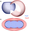 |
Fig. 1. Yin-Yang grid used in our simulation. (a) Three-dimensional view of the Yin and Yang grids. The blue and red lines show the Yin and Yang coordinates, respectively. (b) Mollweide projection of the Yin-Yang grid. The thick black curve denotes the location where the horizontal boundary condition is set in our code. |
 (10)
(10)
and on the curve 𝒞′,
![Mathematical equation: $$ \begin{aligned} \mathcal{C}^\prime :\left\{ \begin{array}{l} \theta^\prime = \cos ^{-1}{\left[\sin {\theta \sin {\phi }}\right]}\\ \phi^\prime = \tan ^{-1}{\left[-\cos {\theta }/ (\sin {\theta }\cos {\phi })\right]} \end{array}, \right. \end{aligned} $$](/articles/aa/full_html/2022/10/aa44150-22/aa44150-22-eq12.gif) (11)
(11)
where (θ, ϕ)∈𝒞. By doing so, the overlapping regions are excluded from our numerical domain. The location where the boundary condition is set on a spherical surface is shown as a thick black curve in Fig. 1b. Both the upper and lower radial boundaries are assumed to be impenetrable and stress-free, and the radial gradient of entropy is assumed to vanish there. The grid resolution is 72(Nr)×96(Nθ)×288(Nϕ)×2 (Yin and Yang). The simulation is initiated from a small random fluctuation in s1. To check whether the results are sensitive to the initial perturbations, we carried out six different simulation runs with different random initial fluctuations. Each simulation run corresponds to about 25 solar years, and we analyze the 15 years of data after the differential rotation becomes statistically stationary (see Appendix A). The data is saved at a time cadence of about 4.7 days. Most results shown in the following sections are averages over six realizations (of 15 years each) to improve the signal-to-noise ratio.
3.2. Extracting modes from simulations
We begin with the simulations where each physical variable is only given for discrete values of r, θ, ϕ, and t. We extract the eigenfunctions of the large-scale low-frequency modes of oscillation from the simulation data using a singular-value decomposition (SVD) similar to what was done by Proxauf et al. (2020). To sketch the method, we consider qα(r, θ, ϕ, t) to be any of the physical variables, vr, vθ, vϕ, s1, or p1. We perform a Fourier transform of these variables to obtain
 (12)
(12)
where m is the azimuthal order and ω is the angular frequency. With this definition, the phase speed ω/m is positive in the direction of rotation (prograde) and negative in the direction opposite to rotation (retrograde). In the following we choose m to be positive with no loss of generality. Each m is analyzed independently.
Among the set of variables {qα}, we choose a particular physical variable qβ to target a particular mode. For example, we choose qβ = uϕ for the columnar convective modes and qβ = uθ for the equatorial Rossby modes and the mixed Rossby modes. Since our main focus is on the modes that peak near the equator, we consider the latitudinal average
 (13)
(13)
over a narrow band of latitudes covering 15° on either side of the equator. Given the mode frequency ωmode for which we want to extract the eigenfunctions, we limit the domain of analysis to the frequency range [ω1, ω2]∋ωmode and to an appropriate radius range [r1, r2] in which the mode has significant power in order to reduce the contamination from the neighboring modes. For each fixed m, the quantity q̃β,eq is then decomposed according to the SVD as
 (14)
(14)
where σk are the singular values, Uk and Vk are the left and right singular vectors, and H denotes the conjugate transpose. The vectors Vk are normalized such that  . The decomposition is ordered such that the first singular value is dominant over the other values. For each mode we keep only the first of the right singular vectors, V0, from the SVD. Using
  derived from qβ, the spatial dependence of a mode is calculated for all the other variables qα according to
 (15)
(15)
These spatial functions are approximations to a mode’s eigenfunctions, and can be compared to the eigenfunctions from the linear analysis. The amplitude of a mode extracted using the above equation is an estimate of the root mean square (rms) of this mode in the frequency range ω1 ≤ ω ≤ ω2, according to Parseval’s theorem.
3.3. Linear eigenvalue solver
The modes extracted from the nonlinear rotating convection simulation were compared to the linear eigenmodes of oscillation in the Sun. To solve the linearized problem, we used the code developed in Bekki et al. (2022). The differences from the Bekki et al. (2022)’s setup are as follows. The lower and upper boundaries are changed to (rmin, rmax)=(0.71 R⊙, 0.96 R⊙) corresponding to those of the nonlinear simulation. We also impose the differential rotation (the axisymmetric background mean flow) taken from the nonlinear simulation (Fig. 2a). However, we do not take into account the meridional circulation, which has a much smaller impact on inertial modes than the differential rotation (Gizon et al. 2020; Fournier et al. 2022). For simplicity, the background is adiabatic (δ = 0) and a spatially uniform viscosity of 1012 cm2 s−1 is included.
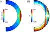 |
Fig. 2. Temporally averaged profile of (a) the differential rotation Ω(r, θ)=Ω0 + ⟨vϕ⟩/rsinθ, and (b) the streamlines of the meridional circulation vm = (⟨vr⟩,⟨vθ⟩). Here ⟨⟩ denotes the longitudinal average. The meridional flow stream function Ψ is defined by ρ0vm = ∇ × (Ψeϕ). Red (blue) indicates the circulation is clockwise (counter-clockwise), i.e., the flow is poleward (equatorward) near the surface at high latitudes in both hemispheres. |
4. General results
4.1. Rossby number regime
We first evaluate the parameter regime of our nonlinear rotating convection simulation. To do so, we compute the volume-averaged rms velocity in the simulation (fluctuations with respect to the mean flows) defined by
![Mathematical equation: $$ \begin{aligned} \overline{v}^2_{\mathrm{rms}} = \frac{1}{V} \int _{V} \ \left[(v_{\rm r}-\langle v_{\rm r} \rangle )^{2} + (v_{\theta }-\langle v_{\theta } \rangle )^{2}+ (v_{\phi }-\langle v_{\phi } \rangle )^{2}\right] \mathrm{d}V, \end{aligned} $$](/articles/aa/full_html/2022/10/aa44150-22/aa44150-22-eq19.gif) (16)
(16)
where ⟨⟩ denotes the azimuthal average, and the integral is taken over the volume of the whole convection zone V. We obtain v̄rms = 37.1 m s−1, which is smaller than that of previous simulations of solar global convection by a factor of about 3 (e.g., Miesch et al. 2008; Hotta et al. 2022). This is due to the fact that the luminosity is reduced by a factor of 20 from the solar value in our simulation.
The rotational influence on convection can be measured by the Rossby number
 (17)
(17)
We obtain Ro = 0.04, indicating that our simulation is operating in a strongly rotationally constrained regime. Thanks to this low Ro, we successfully obtain the solar-like differential rotation (with faster equator and slower poles; see Gastine et al. 2013). Whether the Rossby number in our simulation takes a realistic value is an open question. The Rossby number in the Sun’s convection zone is one of the most important unknown global parameters, which bears on the solar convective conundrum.
4.2. Axisymmetric mean flows
Figures 2a and b show the time-averaged profiles of the axisymmetric mean flows (i.e., differential rotation and meridional circulation, respectively). For the parameters we used the differential rotation is solar-like, although its amplitude is much weaker than that of the real Sun (e.g., Howe 2009). The reference rotation rate of Ω0/2π = 431.3 nHz roughly corresponds to the middle-latitude rotation rate (≈40°) at the surface. The meridional flow tends to have a multiple-cellular structure at low latitudes, but is largely counter-clockwise (clockwise) in the northern (southern) hemisphere at higher latitudes: The flow at high latitudes is poleward (equatorward) at the surface (base of the convection zone) (e.g., Featherstone & Miesch 2015).
5. Low-frequency modes found in our simulation
5.1. Columnar convective modes
Figures 3a and b show temporal snapshots of the nonaxisymmetric components respectively of radial velocity vr and longitudinal velocity vϕ near the surface r = 0.95 R⊙. The convective structure at high latitudes can be characterized by granular cells consisting of broad upflows and narrow downflows (e.g., Spruit et al. 1990). Near the equator we can clearly see the north-south aligned lanes of radial and longitudinal velocities. They are often called banana cells and have been repeatedly reported in previous numerical simulations of rotating convection (Miesch et al. 2000; Käpylä et al. 2011, 2019; Gastine et al. 2013; Guerrero et al. 2013; Hotta et al. 2015a; Featherstone & Hindman 2016; Matilsky et al. 2019, 2020). We show that these banana cell features can be identified as the columnar convective modes largely originating from the compressional β-effect (Glatzmaier & Gilman 1981; Glatzmaier et al. 2009; Verhoeven & Stellmach 2014; Bekki et al. 2022).
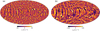 |
Fig. 3. Snapshots of the convective pattern in our simulation near the top boundary r = 0.95R⊙. Panels a and b: radial velocity vr and nonaxisymmetric component of the longitudinal velocity vϕ. |
Figure 4a shows the equatorial power spectrum (m − ω diagram) of the longitudinal velocity near the top boundary |ṽϕ,eq(0.95 R⊙,m,ω)|2. The dispersion relationship for the columnar convective modes from the linear eigenmode calculation is overplotted in red. The frequencies are given for a frame rotating with Ω0. A clear power ridge can be observed in Fig. 4a, matching that from the linear analysis for m ≲ 10. The frequency of this power ridge is positive in the frame rotating with the local differential rotation rate (denoted by blue solid line), implying that the convective modes are propagating in a prograde direction (Miesch et al. 2008; Bessolaz & Brun 2011). Figure 4b shows the same equatorial power spectrum at fixed azimuthal order |ṽϕ,eq(r,m = 8,ω)|2. The strong longitudinal velocity power is localized near the surface where the compressional β-effect ( where Hρ is the density scale height) is the strongest (e.g., Glatzmaier & Gilman 1981). At m = 8, the mode has a linewidth of 30 nHz and a corresponding decaying timescale of 122 days.
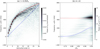 |
Fig. 4. Equatorial power spectra of longitudinal velocity vϕ. (a) The power spectrum near the top boundary r = 0.95 R⊙. The power is normalized at each m. The spectrum is computed in a frame rotating at Ω0/2π = 431.3 nHz (the rotation rate of the radiative interior). The blue line represents the advective speed by the local differential rotation, m[Ω(0.95R⊙,π/2)−Ω0]. Overplotted in red is the dispersion relation of the columnar convective modes from the linear eigenmode calculation. (b) Same equatorial power spectrum as in (a), but at fixed azimuthal order m = 8 as a function of depth. The blue line is again the local advection frequency and the red line is the eigenfrequency from the linear analysis. |
We used the method described in Sect. 3.2 to extract the spatial structure of the columnar convective modes for azimuthal orders 1 ≤ m ≤ 391. To extract the modes, we calculated V0(m, ω) in Eq. (15) based on the equatorial spectrum of longitudinal velocity near surface. Figure 5 shows the three-dimensional spatial patterns of the convective columnar modes found in our simulation for selected m. For visualization purposes, the nonaxisymmetric components of pressure perturbation p1 are shown. We note that the positive (negative) pressure perturbation p1 is associated with negative (positive) z-vorticity ζz of the modes due to the strong constraint of geostrophic balance (e.g., Matilsky et al. 2020). It is clearly seen that the columnar convective modes are characterized by the north-south aligned columns across the equatorial plane.
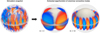 |
Fig. 5. Three-dimensional visualization of the columnar convective modes. Left: snapshot of pressure perturbation (nonaxisymmetric component) from the nonlinear simulation shown as a 3D volume rendering. The red-yellow and blue-cyan parts correspond to the regions with positive and negative pressure perturbations, respectively. Right: eigenfunctions of pressure perturbation of the columnar convective modes extracted from the simulation data using SVD. The cases with m = 2 and m = 12 are shown. |
Figure 6 shows the extracted eigenfunctions of the convective columnar modes for m = 2, in comparison with the results of the linear analysis. The real eigenfunctions of vr and vθ and the imaginary eigenfunctions of vϕ and p1 are shown in Fig. 6a. Figures 6b and c further compare the radial and latitudinal structures of the extracted mode at the equator and at the surface, respectively. We note that the eigenfunctions extracted from the simulations are realizations of random processes, and therefore contain noise. The noise is visible at small spatial scales; however, particularly at large scales, a great agreement can be seen between the eigenfunctions from the simulation and those of the linear analysis. Therefore, the columnar convective modes are unambiguously identified in our simulations. The modes can be clearly characterized by a dominant z-vorticity ζz that is confined outside the tangential cylinder as described in detail in Bekki et al. (2022). As m increases, the eigenfunctions are more and more confined toward the surface and toward the equator (not shown).
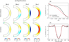 |
Fig. 6. Spatial eigenfunctions qα, mode(r, θ, m) for the ζz-symmetric columnar convective modes with m = 2. By definition, modes are of the form qα, mode(r, θ, m)exp[i(mϕ−ωt)], where qα is either vr, vθ, vϕ, or p1. (a) Meridional cuts of the radial velocity vr, latitudinal velocity vθ, longitudinal velocity vϕ, and pressure perturbation p1 extracted from the convection simulation (lower panels) and obtained from our linear calculation (upper panels). (b) Radial dependence of the eigenfunction vϕ at the equator. The black solid and red dashed lines represent the simulation and linear calculation, respectively. (c) Latitudinal eigenfunction of vϕ at the surface normalized near the equator. |
5.2. Equatorial Rossby modes
In this section we present the same modal analysis for the equatorial Rossby modes (r modes) where the radial vorticity ζr is symmetric across the equator. In this study, we use the latitudinal velocity vθ near the equator for our spectral analysis which is a good representative of the equatorial Rossby modes. Figures 7a and b show the equatorial power spectra (m − ω diagram) of latitudinal velocity near the base |ṽϕ,eq(0.75 R⊙,m,ω)|2 and near the surface |ṽϕ,eq(0.95 R⊙,m,ω)|2, respectively. The dispersion relation of the equatorial Rossby modes with no radial node (n = 0) obtained from our linear analysis is shown in red points in Fig. 7a. A clear power ridge can be seen along the linear dispersion relation near the base, whereas two distinct ridges are found in the surface power spectrum (denoted as “mixed prograde” and “mixed retrograde” in Fig. 7b).
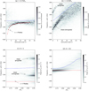 |
Fig. 7. Power spectra of latitudinal velocity vθ near the equator (averaged over ±15 deg). Panels a and b: m − ω diagram near the base (r = 0.75 R⊙) and near the surface (r = 0.95 R⊙), respectively. The power is normalized at each m. The spectra are computed in a frame rotating at Ω0/2π = 431.3 nHz. Overplotted in red line in panel a is the dispersion relation of the equatorial Rossby mode with no radial node (n = 0) obtained from the linear calculation. The blue line represents the advection frequency of the equatorial differential rotation, m[Ω(r,π/2)−Ω0], at each height. Panels c and d: power spectra at fixed azimuthal order m = 1 and m = 16, respectively. |
Figures 7c and d show the same equatorial power spectra of vθ at fixed azimuthal orders |ṽϕ,eq(r,m = 1,ω)|2 and |ṽϕ,eq(r,m = 16,ω)|2, respectively. As shown in Fig. 7c, three distinct modes exist at low-m regime:
-
A retrograde-propagating mode that exists globally in radius at ω/2π ≈ −395 nHz. Its mode frequency is close to the theoretical eigenfrequency of the n = 0 Rossby mode predicted in linear analysis (denoted by red line) and is independent of height. This mode is clearly identified as the n = 0 equatorial Rossby mode, and is discussed in Sect. 5.2.1.
-
A retrograde-propagating mode localized near the surface at ω/2π ≈ −230 nHz is also seen. This mode is identified as the equatorial Rossby mode with one radial node (n = 1) and is discussed in Sect. 5.3.
-
A prograde-propagating mode localized near the surface at ω/2π ≈ 320 nHz is also apparent. This mode is identified as the north-south ζz-antisymmetric columnar convective mode and is also discussed in Sect. 5.3.
At higher m, on the other hand, most of the power is concentrated near the bottom convection zone at frequencies close to those of the n = 0 Rossby modes from the linear analysis (red line in Fig. 7d). The properties of these high-m Rossby modes are discussed in Sect. 5.2.2.
5.2.1. Rossby modes with n = 0 and m ≤ 4
At low m, equatorial Rossby modes can be unambiguously found in our simulation. Figure 8a shows the extracted eigenfunctions of m = 2 mode as an example. The associated flow motion is mostly r-vortical and quasi-toroidal (i.e., vr ≈ 0). Geostrophical balance is well established by positive (negative) p1 in a region where ζr is negative (positive) in the northern (southern) hemisphere. The radial component of the Coriolis force is balanced by the radial pressure gradient force. For m ≤ 4, almost all the power is in the real part of the eigenfunction for vθ (ℜ[vθ]) and the imaginary part for vϕ (ℑ[vϕ]). The other components of the eigenfunctions (for example ℑ[vθ] or ℜ[vϕ]) are small and consistent with noise. For comparison, we also show the eigenfunctions of the m = 2 equatorial Rossby mode with no radial node (n = 0) obtained from our linear calculation in the upper panel of Fig. 8a. A very good agreement can be seen between the extracted eigenfunctions from the nonlinear simulation and those of the linear calculation. Figures 8b and c further compare the radial and latitudinal structures of the eigenfunction of vθ. The radial eigenfunction roughly shows a monotonic increase toward the surface as expected from the analytical solution for the ideal case of inviscid and uniformly rotating sphere, vθ ∝ rm (e.g., Saio 1982). Similarly, the latitudinal eigenfunction also roughly follows the analytical solution for the ideal case, vθ ∝ sinm − 1θ.
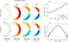 |
Fig. 8. Eigenfunctions of the equatorial Rossby mode with no radial node (n = 0) for m = 2. (a) Meridional eigenfunctions extracted from the simulation (lower panels) and those obtained from the linear analysis (upper panels). The same notation is used as in Fig. 6a. (b) Radial eigenfunction of vθ at the equator. The black solid and red dashed lines show the results from the simulation and linear calculation, respectively. (c) Latitudinal eigenfunction of vθ in the middle convection zone. |
It is noteworthy that the m = 1 equatorial Rossby mode shown in Fig. 7c has a flow vorticity that is uniform in the frame of the mode and points in a direction perpendicular to the solar rotation axis. This particular mode is often called the spin-over inertial mode (e.g., Greenspan et al. 1968) and has been extensively studied in the context of planetary cores (e.g., Triana et al. 2012; Rekier 2022).
We also note that these equatorial Rossby modes at low m are very long-lived. For instance, the m = 4 mode has a linewidth of 7.5 nHz, which corresponds to a lifetime of about 500 days. The modes with m < 4 have much longer lifetimes as their linewidths are too small to be well resolved and to be fitted with a Lorentzian.
5.2.2. Rossby modes with n = 0 and m > 4
As m increases, the eigenfunctions of the n = 0 equatorial Rossby modes significantly deviate from the well-known analytical expression of vθ ∝ rmsinm − 1θ. Figure 9 shows the eigenmode at m = 24 that is extracted from the convection simulation along the power ridge shown in Fig. 7a. We note that the eigenfunctions become essentially complex, with the complex phase for each variable being a function of r and θ. For large azimuthal order m, the modes cease to be quasi-toroidal; in other words, the radial motions become substantial and the modes are partially convectively driven. This can be confirmed in Fig. 9, where vr and s1 have the same sign at the same phase in both hemispheres. The transport properties of thermal energy is discussed in detail in Sect. 6.2.
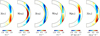 |
Fig. 9. Extracted eigenfunctions of the n = 0 equatorial Rossby modes at m = 24. Eigenfunctions of radial velocity (imaginary) ℑ[vr], latitudinal velocity (real) ℜ[vθ] and (imaginary) ℑ[vθ], longitudinal velocity (real) ℜ[vϕ], pressure perturbation (real) ℜ[p1], and entropy perturbation (imaginary) ℑ[s1] are shown from left to right. The real and imaginary phases are determined in a way such that ℜ[vθ] at the base takes its maximum at the equator. |
It is also found that the n = 0 Rossby modes are more and more confined toward the base of the convection zone as m increases. This is clearly illustrated in Fig. 10 where the normalized eigenfunctions of ℜ[vθ] at the equator are plotted against radius for different m. For m ≥ 4 the radial eigenfunctions become decreasing functions in radius, which clearly disagrees with the analytical solution of Rossby modes in the ideal case (uniform rotation and no viscosity; Saio 1982). In the ideal case rm dependence is required in order to balance the radial component of the Coriolis force by the radial pressure gradient. We attribute this discrepancy to the strong viscous diffusion in our simulation; when strong diffusivity is present, the radial force balance is drastically changed. This has already been pointed out by Bekki et al. (2022) who showed, in the linear regime, that the eigenfunctions of n = 0 Rossby modes tend to be localized near the base of the convection zone when the turbulent viscosity is above ≈1012 cm2 s−1. To confirm this, we show in Fig. 10 the results from our linear calculations (dashed lines) that can clearly explain this trend. The effective diffusivity in our nonlinear simulation is substantially enhanced by the turbulent (eddy) momentum mixing by the convective flows. In Appendix B we estimate the turbulent diffusivity due to the small-scale convective motions in the simulation to be ≈3 × 1012 cm2 s−1 throughout the convection zone, which is larger than the explicit viscosity value of 1012 cm2 s−1. Therefore, the effective viscosity is dominated by the eddy diffusion due to the stochastic convective motions on resolved scales. For more detailed discussions on the effect of turbulent diffusion on Rossby modes, see Sect. 5 in Bekki et al. (2022).
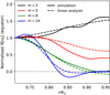 |
Fig. 10. Radial structure of the real eigenfunctions of latitudinal velocity ℜ[vθ] at the equator. The eigenfunctions are normalized to unity at the base. The different colors represent different azimuthal orders m (see inset). The solid and dashed lines denote the eigenfunctions extracted from the nonlinear simulation and from the linear eigenmode calculation, respectively. |
Figure 9 also reveals that at high m the flow motions are characterized by z-vortices along with the tangential cylinder, as manifested by the eigenfunctions of ℑ[vr], ℑ[vθ], and ℜ[vϕ]. The essential difference from the columnar convective modes discussed in Sect. 5.1 is that here ζz is north-south antisymmetric across the equator. This is schematically illustrated in Fig. 11. These modes should also be distinguished from the prograde-propagating mixed Rossby modes (see Sect. 5.3), where the power is strongly localized near the surface and not at the tangential cylinder.
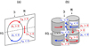 |
Fig. 11. Schematic illustration of the flow structure of the n = 0 equatorial Rossby modes at (a) low-m and (b) high-m regimes. |
It should be noted that these high-m equatorial Rossby modes generally have broader linewidths (thus shorter lifetimes) than those with low m. For instance, the mode with m = 15 has a linewidth of about 25 nHz. This is in fact comparable to those observed in the Sun (the linewidth of the m = 15 mode observed on the Sun is reported to be ≈10 − 40 nHz; see Löptien et al. 2018; Liang et al. 2019; Proxauf et al. 2020).
5.3. Mixed Rossby modes
Figure 12a shows the same equatorial power spectrum near the surface as Fig. 7b, except that we extend the spectrum to negative azimuthal orders (m < 0) considering the symmetry with respect to the origin: |ṽϕ,eq(−m,−ω)|2 = |ṽϕ,eq(m,ω)|2. We also show the equatorial power spectrum of the north-south antisymmetric component of vϕ in Fig. 12b. We note that both Fig. 12a and b have the same symmetry, and thus represent the same modes. This enables us to more clearly see the connection between the two distinct power ridges that are denoted as mixed retrograde and mixed prograde. These two oppositely propagating modes form a single continuous power ridge across m = 0, implying that they are essentially mixed with each other. The axisymmetric mode (m = 0) is considered to be an inertial mode trapped inside the spherical shell (e.g., Rieutord 2001; Rieutord & Valdettaro 2018) and has an oscillation frequency of about ω/2π ≈ ±280 nHz.
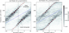 |
Fig. 12. Power spectra of horizontal velocities near the surface extended to negative azimuthal orders (m < 0). (a) Equatorial power spectrum of north-south symmetric component of vθ near the top boundary r = 0.95 R⊙, which is the same as Fig. 7b. The power is normalized at each m. Shown in red points are the frequencies of the mixed Rossby modes obtained from our linear analysis. The blue line represents the advection frequency of the equatorial differential rotation, m[Ω(0.95 R⊙,π/2)−Ω0]. (b) Equatorial power spectrum of north-south antisymmetric component of vϕ near the top boundary r = 0.95 R⊙. |
Figure 13a shows the extracted eigenfunctions of the retrograde-propagating mode at m = 2. The retrograde-propagating mode can be classified as an equatorial Rossby mode with one radial node n = 1 in the middle convection zone, as depicted in Fig. 13b. We note that the nodal plane is more cylindrical than radial outside the tangential cylinder. The associated motion is dominantly r-vortical near the surface, but unlike the n = 0 equatorial Rossby modes, non-negligible radial velocities are involved. Similarly, the extracted eigenfunctions of the prograde-propagating mode at m = 2 are shown in Fig. 14a. The prograde-propagating mode can be classified as a north-south ζz-antisymmetric columnar convective mode, as illustrated in Fig. 14b. Given that both of these modes follow the same dispersion relationship, we call them mixed Rossby modes in this paper.
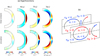 |
Fig. 13. Eigenfunctions of the retrograde-propagating mixed Rossby mode (n = 1 equatorial Rossby mode). (a) Meridional cuts of the eigenfunctions at m = 2. The lower and upper panels respectively show the results extracted from the simulation and from the linear analysis. (b) Schematic illustration of this mode. |
The existence of the mixed Rossby modes was first pointed out in Bekki et al. (2022). Their dispersion relation asymptotically approaches that of the n = 0 equatorial Rossby mode for large m with negative ω (retrograde modes) and to that of the north-south ζz-symmetric columnar convective mode for large m with positive ω (prograde modes). The coupling between these two oppositely propagating modes can be understood by analogy to the well-known mixed Rossby-gravity waves (sometimes called Yanai waves) in the geophysical context (e.g., Matsuno 1966; Vallis 2006) whose dispersion relation is asymptotic to that of classical Rossby waves for large m with negative ω (retrograde) and asymptotic to that of inertia-gravity waves for large m with positive ω (prograde).
To further support the identification of these mixed Rossby modes, we compute the dispersion relation and the corresponding eigenfunctions using the linear eigenvalue solver. The computed dispersion relation is shown by red points in Fig. 12 for m ≤ 5, which nicely agrees with the power ridge in the simulated spectrum. We also show in Figs. 13a and 14a the eigenfunctions of the n = 1 equatorial Rossby mode and the north-south ζz-antisymmetric columnar convective mode at m = 2 obtained from the linear calculation. The agreement between the simulation and linear theory is striking.
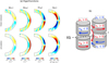 |
Fig. 14. Eigenfunctions of the prograde-propagating mixed Rossby mode (north-south ζz-antisymmetric columnar convective mode). (a) Meridional cuts of the eigenfunctions at m = 2. Lower and upper panels: respectively show the results extracted from the simulation and from the linear analysis. (b) Schematic illustration of this mode. |
6. Transport properties of low-frequency modes
6.1. Mode amplitudes
So far we have investigated the eigenfunctions and eigenfrequencies of the north-south ζz-symmetric columnar convective modes, the n = 0 equatorial Rossby modes, and the mixed Rossby modes. In this section we discuss how significant these modes are for transport processes in our nonlinear simulation.
Figure 15a shows the spectra of the maximum horizontal velocity  of the equatorial modes near the surface. It is clearly seen that the north-south ζz-symmetric columnar convective modes are the most dominant in power; they account for about 10 − 30% of the total velocity power of the simulation near the surface (black dashed line). When observed at the surface, the n = 0 equatorial Rossby modes are much weaker than the columnar convective modes and the mixed Rossby modes. Nonetheless, their amplitudes are comparable to those observed on the Sun (Liang et al. 2019; Gizon et al. 2021). This may imply that these equatorial Rossby modes are both excited and damped by the turbulent convective motions.
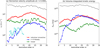 |
Fig. 15. Spectra of the equatorial modes. (a) Maximum horizontal velocity vh of the equatorial modes near the top boundary r = 0.95 R⊙ at each azimuthal order m. The red, blue, and green points represent the ζz-symmetric columnar convective modes, n = 0 equatorial Rossby modes, and the mixed Rossby modes, respectively. The black dashed line represents the overall power of the convection simulation (including modes at high latitudes and stochastic convective motions). The cyan diamonds and squares denote the (rms) horizontal velocity amplitudes of the observed Rossby modes near the solar surface obtained by Liang et al. (2019) and Gizon et al. (2021), respectively. (b) Spectra of the volume-integrated kinetic energy of the equatorial modes. |
Figure 15b shows, on the other hand, the spectra of the volume-integrated kinetic energies of these modes. It can be seen that, despite the weak amplitudes in the surface spectrum, the total kinetic energy of the n = 0 equatorial Rossby modes become significant; it is much greater than that of the mixed modes for m > 6, and become comparable to that of the ζz-symmetric columnar convective modes for m ≥ 10. This reflects that the n = 0 Rossby modes are concentrated near the base of the convection zone at high m where the background density is substantial. As shown in Col. 2 of Table 1, the ζz-symmetric columnar convective modes and the n = 0 Rossby modes have about 7% and 6% of the total fluctuating (m ≠ 0) kinetic energy of the simulation, respectively.
Amplitudes and lifetimes of the equatorial vorticity modes in our simulation.
6.2. Thermal energy transport
To examine the properties of the thermal energy transport, we compute the (radial) enthalpy flux Fe for each extracted mode as
 (18)
(18)
where ⟨⟩ denotes the longitudinal average and T1 is temperature perturbation
![Mathematical equation: $$ \begin{aligned} T_{1}=\left[\frac{\gamma -1}{\gamma }\frac{p_{1}}{p_{0}} +\frac{s_{1}}{c_{\rm p}}\right] T_{0}. \end{aligned} $$](/articles/aa/full_html/2022/10/aa44150-22/aa44150-22-eq25.gif) (19)
(19)
Figures 16a–c show meridional distributions of the enthalpy flux Fe for the three extracted vorticity modes summed over m = 1 − 39. We note that all of these modes transport the thermal energy radially upward. The ζz-symmetric columnar convective modes transport about 65% of what is required in the upper convection near the equator. The n = 0 Rossby modes and the mixed modes can transport about 8 − 9% of the required thermal energy in the lower and upper convection zone, respectively, outside the tangential cylinder.
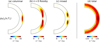 |
Fig. 16. Enthalpy fluxes Fe associated with the extracted modes in our simulations summed over m = 1 − 39. Panels a–c: ζz-symmetric columnar convective modes, the n = 0 equatorial Rossby modes, and the mixed Rossby modes, respectively. Panel d: the total enthalpy flux (including other modes and small-scale convection) is shown. The fluxes are normalized by the injected energy flux F* = L*/(4πr2). |
This is a striking result because the n = 0 Rossby modes are believed to be quasi-toroidal and cannot contribute to the thermal energy transport in the linear theory for the simplified case with uniform rotation, no turbulent diffusion, and adiabatic background stratification (e.g., Saio 1982; Damiani et al. 2020). We find that, under the influence of strong turbulent diffusion and superadiabatic background, the n = 0 equatorial Rossby modes become partially convective, especially at high m.
6.3. Angular momentum transport
These equatorial vorticity modes also transport the angular momentum. Figures 17a–c show the Reynolds stresses ρ0⟨vrvϕ⟩ (upper panels) and ρ0⟨vθvϕ⟩ (lower panels) summed over all m values for the extracted ζz-symmetric columnar convective modes, n = 0 equatorial Rossby modes, and the mixed Rossby modes, respectively. These terms are proportional to the radial and latitudinal components of the convective angular momentum flux. For comparison, we show the total Reynolds stresses in our simulation (which include contributions from the other modes and small-scale convection) in Fig. 17d.
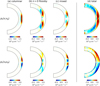 |
Fig. 17. Reynolds stresses associated with the extracted modes in our simulations summed over m = 1 − 39. Panels a–c: ζz-symmetric columnar convective modes, the n = 0 equatorial Rossby modes, and the mixed Rossby modes, respectively. Panel d: the total Reynolds stresses (including other modes and small-scale convection) is shown. Upper and lower panel: respectively corresponds to ρ0⟨vrvϕ⟩ and ρ0⟨vθvϕ⟩. |
For the radial transport of the angular momentum, the dominant contribution is from the ζz-symmetric columnar convective modes, which is about eight times bigger than those from the n = 0 Rossby modes and the mixed Rossby modes. The radially upward angular momentum flux by the columnar convective modes accounts for about 37% of the total amount in the upper half of the convection zone near the equator. The positive ⟨vrvϕ⟩ outside the tangential cylinder is a common feature of convection simulation in a strongly rotationally constrained regime (Gastine et al. 2013; Fan & Fang 2014; Hotta et al. 2015a; Matilsky et al. 2020).
On the other hand, the angular momentum is preferentially transported equatorward in our simulation, as manifested by positive (negative) ⟨vθvϕ⟩ in the northern (southern) hemisphere in the lower panel of Fig. 17d. Our analysis reveals that both the ζz-symmetric columnar convective modes and the n = 0 Rossby modes contribute to this net equatorward angular momentum transport by about 30 − 40% near the surface and at the base, respectively. The mixed Rossby modes turn out to be rather insignificant for the net angular momentum transport in the latitudinal direction.
7. Summary and discussion
In this paper we reported a mode-by-mode analysis of the low-frequency equatorial vorticity modes in a fully nonlinear simulation of solar-like rotating convection. This study was motivated by the recent observational discovery of various types of inertial modes on the Sun (Löptien et al. 2018; Gizon et al. 2021) and the consequent theoretical study on these modes in a linear regime (Bekki et al. 2022).
Based on the equatorial velocity power spectra, we successfully identified and characterized several types of equatorial modes in our simulation. For each mode eigenfunctions are extracted using the SVD method. We also carried out a linear eigenmode analysis with the simulated differential rotation included. The computed linear dispersion relations and eigenfunctions are compared with the simulated power spectra and the extracted eigenfunctions. Our work provides a technique for subsequent numerical studies of low-frequency inertial modes in nonlinear convection simulations.
We successfully identified the ζz-symmetric columnar convective modes, the n = 0 equatorial Rossby modes, and the mixed Rossby modes. Table 1 summarizes the modes identified in this paper. Although we mainly focused on these equatorial modes in this paper, we also checked that the high-latitude modes exist in our simulation as well (see Appendix C).
Our major findings can be summarized as follows. The north-south ζz-symmetric columnar convective modes have the highest power in our simulation. They originate primarily from the compressional β-effect near the surface, and thus can be well characterized by the dispersion relation similar to that of Glatzmaier & Gilman (1981). They transport a significant fraction of enthalpy upward and are the dominant term in the angular momentum transport near the equator.
Our analysis reveals, at high m, that the equatorial Rossby modes with no radial nodes (n = 0) have eigenfunctions that deviate from that of the uniformly rotating inviscid case. As m increases, we find that these modes are more and more confined near the base of the convection zone. We argue that this is due to the strong diffusion arising from the turbulent convective motions on resolved scales, which breaks the radial force balance between the pressure gradient and the Coriolis force and drives radial flows (Bekki et al. 2022). We find that these equatorial Rossby modes are the longest-lived modes in our simulation.
Mode mixing between the equatorial Rossby modes and the columnar convective modes is found in our nonlinear simulations, as predicted by the linear analysis of Bekki et al. (2022). The surface power spectrum of the north-south symmetric vθ can be characterized by two oppositely propagating modes that form a single well-defined power ridge across m = 0. The retrograde and prograde modes for m > 0 can be identified as the n = 1 equatorial Rossby modes and the north-south ζz-antisymmetric columnar convective modes, respectively. We call them mixed Rossby modes, following Bekki et al. (2022). An analogy can be drawn between these mixed modes and the Yanai waves (mixed Rossby-gravity waves), where the retrograde-propagating Rossby waves and prograde-propagating gravity waves (Kelvin waves) are mixed with one another (e.g., Vallis 2006). The existence of the mixed Rossby modes has important implications. One of these follows from its frequency, which is very close to that of the n = 0 equatorial Rossby mode at m ≥ 5 (see Fig. 10 in Bekki et al. 2022). Therefore, it is possible that the observed Rossby modes on the Sun could be n = 1 modes rather than n = 0 modes as is typically assumed.
The nonlinear simulations contain a wealth of information about many more modes of oscillations in the inertial frequency range. The analysis method reported in this paper can be used in the future to study the m = 1 high-latitude inertial mode (Gizon et al. 2021; Bekki et al. 2022) and the l = m + 1 high-frequency retrograde modes (Hanson et al. 2022).
The maximum azimuthal order in our grid resolution is 192. However, we restrict our analysis to large-scale modes in a range 0 ≤ m ≤ 39.
Acknowledgments
We thank an anonymous referee for constructive comments. Y.B. is enrolled in the International Max-Planck Research School for Solar System Science at the University of Göttingen (IMPRS). Y.B. also acknowledges a financial support from long-term scholarship program for degree-seeking graduate students abroad from the Japan Student Services Organization (JASSO). We acknowledge a support from ERC Synergy Grant WHOLE SUN 810218 and the hospitality of the Institut Pascal in March 2022. All the numerical computations were performed at GWDG and the Max-Planck supercomputer RZG in Garching.
References
- Balbus, S. A., Bonart, J., Latter, H. N., & Weiss, N. O. 2009, MNRAS, 400, 176 [NASA ADS] [CrossRef] [Google Scholar]
- Baruteau, C., & Rieutord, M. 2013, J. Fluid. Mech., 719, 47 [NASA ADS] [CrossRef] [Google Scholar]
- Bekki, Y., & Yokoyama, T. 2017, ApJ, 835, 9 [NASA ADS] [CrossRef] [Google Scholar]
- Bekki, Y., Hotta, H., & Yokoyama, T. 2017, ApJ, 851, 74 [NASA ADS] [CrossRef] [Google Scholar]
- Bekki, Y., Cameron, R. H., & Gizon, L. 2022, A&A, 662, A16 [NASA ADS] [CrossRef] [EDP Sciences] [Google Scholar]
- Bessolaz, N., & Brun, A. S. 2011, ApJ, 728, 115 [NASA ADS] [CrossRef] [Google Scholar]
- Bogart, R. S., Baldner, C. S., & Basu, S. 2015, ApJ, 807, 125 [NASA ADS] [CrossRef] [Google Scholar]
- Brandenburg, A. 2016, ApJ, 832, 6 [Google Scholar]
- Brun, A. S., Miesch, M. S., & Toomre, J. 2004, ApJ, 614, 1073 [Google Scholar]
- Busse, F. H. 1970, J. Fluid. Mech., 44, 441 [NASA ADS] [CrossRef] [Google Scholar]
- Busse, F. H. 2002, Phys. Fluids, 14, 1301 [NASA ADS] [CrossRef] [Google Scholar]
- Busse, F. H., & Or, A. C. 1986, J. Fluid. Mech., 166, 173 [NASA ADS] [CrossRef] [Google Scholar]
- Damiani, C., Cameron, R. H., Birch, A. C., & Gizon, L. 2020, A&A, 637, A65 [EDP Sciences] [Google Scholar]
- Evonuk, M. 2008, ApJ, 673, 1154 [NASA ADS] [CrossRef] [Google Scholar]
- Evonuk, M., & Samuel, H. 2012, Earth Planet. Sci. Lett., 317, 1 [CrossRef] [Google Scholar]
- Fan, Y., & Fang, F. 2014, ApJ, 789, 35 [NASA ADS] [CrossRef] [Google Scholar]
- Featherstone, N. A., & Hindman, B. W. 2016, ApJ, 830, L15 [Google Scholar]
- Featherstone, N. A., & Miesch, M. S. 2015, ApJ, 804, 67 [Google Scholar]
- Fournier, D., Gizon, L., & Hyest, L. 2022, A&A, 664, A6 [NASA ADS] [CrossRef] [EDP Sciences] [Google Scholar]
- Gastine, T., Wicht, J., & Aurnou, J. M. 2013, Icarus, 225, 156 [Google Scholar]
- Gilman, P. A. 1986, in Physics of the Sun., eds. P. A. Sturrock, T. E. Holzer, D. M. Mihalas, & R. K. Ulrich, 1, 95 [NASA ADS] [CrossRef] [Google Scholar]
- Gilman, P. A., & Glatzmaier, G. A. 1981, ApJS, 45, 335 [CrossRef] [Google Scholar]
- Gizon, L., & Birch, A. C. 2012, Proc. Natl. Acad. Sci., 109, 11896 [Google Scholar]
- Gizon, L., Fournier, D., & Albekioni, M. 2020, A&A, 642, A178 [NASA ADS] [CrossRef] [EDP Sciences] [Google Scholar]
- Gizon, L., Cameron, R. H., Bekki, Y., et al. 2021, A&A, 652, L6 [NASA ADS] [CrossRef] [EDP Sciences] [Google Scholar]
- Glatzmaier, G. A. 1984, J. Comput. Phys., 55, 461 [NASA ADS] [CrossRef] [Google Scholar]
- Glatzmaier, G. A., & Gilman, P. A. 1981, ApJS, 45, 381 [NASA ADS] [CrossRef] [Google Scholar]
- Glatzmaier, G., Evonuk, M., & Rogers, T. 2009, Geophys. Astrophys. Fluid Dyn., 103, 31 [NASA ADS] [CrossRef] [Google Scholar]
- Greenspan, H., Batchelor, C., Ablowitz, M., et al. 1968, The Theory of Rotating Fluids (Cambridge: Cambridge University Press) [Google Scholar]
- Guerrero, G., Smolarkiewicz, P. K., Kosovichev, A. G., & Mansour, N. N. 2013, ApJ, 779, 176 [NASA ADS] [CrossRef] [Google Scholar]
- Hanasoge, S., & Mandal, K. 2019, ApJ, 871, L32 [Google Scholar]
- Hanasoge, S. M., Duvall, T. L., & Sreenivasan, K. R. 2012, Proc. Natl. Acad. Sci., 109, 11928 [Google Scholar]
- Hanasoge, S. M., Hotta, H., & Sreenivasan, K. R. 2020, Sci. Adv., 6, eaba9639 [NASA ADS] [CrossRef] [Google Scholar]
- Hanson, C. S., Gizon, L., & Liang, Z.-C. 2020, A&A, 635, A109 [EDP Sciences] [Google Scholar]
- Hanson, C. S., Hanasoge, S., & Sreenivasan, K. R. 2022, Nat. Astron., 6, 708 [NASA ADS] [CrossRef] [Google Scholar]
- Hathaway, D. H., & Upton, L. A. 2021, ApJ, 908, 160 [NASA ADS] [CrossRef] [Google Scholar]
- Hathaway, D. H., Upton, L., & Colegrove, O. 2013, Science, 342, 1217 [NASA ADS] [CrossRef] [Google Scholar]
- Hindman, B. W., & Jain, R. 2022, ApJ, 932, 68 [NASA ADS] [CrossRef] [Google Scholar]
- Hindman, B. W., Featherstone, N. A., & Julien, K. 2020, ApJ, 898, 120 [NASA ADS] [CrossRef] [Google Scholar]
- Hotta, H., Rempel, M., & Yokoyama, T. 2014, ApJ, 786, 24 [NASA ADS] [CrossRef] [Google Scholar]
- Hotta, H., Rempel, M., & Yokoyama, T. 2015a, ApJ, 798, 51 [Google Scholar]
- Hotta, H., Rempel, M., & Yokoyama, T. 2015b, ApJ, 803, 42 [NASA ADS] [CrossRef] [Google Scholar]
- Hotta, H., Kusano, K., & Shimada, R. 2022, ApJ, 933, 199 [NASA ADS] [CrossRef] [Google Scholar]
- Howe, R. 2009, Liv. Rev. Sol. Phys., 6, 1 [Google Scholar]
- Ingersoll, A. P., & Pollard, D. 1982, Icarus, 52, 62 [NASA ADS] [CrossRef] [Google Scholar]
- Kageyama, A., & Sato, T. 2004, Geochem. Geophys. Geosyst., 5, Q09005 [Google Scholar]
- Käpylä, P. J., Mantere, M. J., & Brandenburg, A. 2011, Astron. Nachr., 332, 883 [CrossRef] [Google Scholar]
- Käpylä, P. J., Käpylä, M. J., & Brandenburg, A. 2014, A&A, 570, A43 [NASA ADS] [CrossRef] [EDP Sciences] [Google Scholar]
- Käpylä, P. J., Viviani, M., Käpylä, M. J., Brandenburg, A., & Spada, F. 2019, Geophys. Astrophys. Fluid Dyn., 113, 149 [CrossRef] [Google Scholar]
- Karak, B. B., Miesch, M., & Bekki, Y. 2018, Phys. Fluids, 30, 046602 [NASA ADS] [CrossRef] [Google Scholar]
- Liang, Z.-C., Gizon, L., Birch, A. C., & Duvall, T. L. 2019, A&A, 626, A3 [NASA ADS] [CrossRef] [EDP Sciences] [Google Scholar]
- Löptien, B., Gizon, L., Birch, A. C., et al. 2018, Nat. Astron., 2, 568 [Google Scholar]
- Mandal, K., & Hanasoge, S. 2020, ApJ, 891, 125 [CrossRef] [Google Scholar]
- Mandal, K., Hanasoge, S. M., & Gizon, L. 2021, A&A, 652, A96 [NASA ADS] [CrossRef] [EDP Sciences] [Google Scholar]
- Matilsky, L. I., Hindman, B. W., & Toomre, J. 2019, ApJ, 871, 217 [NASA ADS] [CrossRef] [Google Scholar]
- Matilsky, L. I., Hindman, B. W., & Toomre, J. 2020, ApJ, 898, 111 [NASA ADS] [CrossRef] [Google Scholar]
- Matsuno, T. 1966, J. Meteorol. Soc. Jpn. Ser. II, 44, 25 [CrossRef] [Google Scholar]
- Miesch, M. S., Elliott, J. R., Toomre, J., et al. 2000, ApJ, 532, 593 [CrossRef] [Google Scholar]
- Miesch, M. S., Brun, A. S., DeRosa, M. L., & Toomre, J. 2008, ApJ, 673, 557 [NASA ADS] [CrossRef] [Google Scholar]
- Moffatt, H. K. 1978, Magnetic Field Generation in Electrically Conducting Fluids (Cambridge: Cambridge University Press) [Google Scholar]
- Muñoz-Jaramillo, A., Nandy, D., & Martens, P. C. H. 2011, ApJ, 727, L23 [NASA ADS] [CrossRef] [Google Scholar]
- Nelson, N. J., Featherstone, N. A., Miesch, M. S., & Toomre, J. 2018, ApJ, 859, 117\pg{\newpage} [Google Scholar]
- O’Mara, B., Miesch, M. S., Featherstone, N. A., & Augustson, K. C. 2016, Adv. Space Res., 58, 1475 [CrossRef] [Google Scholar]
- Ong, H., & Roundy, P. E. 2020, J. Atmos. Sci., 77, 3721 [NASA ADS] [CrossRef] [Google Scholar]
- Papaloizou, J., & Pringle, J. E. 1978, MNRAS, 182, 423 [NASA ADS] [CrossRef] [Google Scholar]
- Provost, J., Berthomieu, G., & Rocca, A. 1981, A&A, 94, 126 [NASA ADS] [Google Scholar]
- Proxauf, B., Gizon, L., Löptien, B., et al. 2020, A&A, 634, A44 [NASA ADS] [CrossRef] [EDP Sciences] [Google Scholar]
- Rekier, J. 2022, PSJ, 3, 133 [NASA ADS] [Google Scholar]
- Rempel, M. 2005, ApJ, 622, 1320 [NASA ADS] [CrossRef] [Google Scholar]
- Rempel, M. 2014, ApJ, 789, 132 [Google Scholar]
- Rieutord, M. 2001, ApJ, 550, 443 [NASA ADS] [CrossRef] [Google Scholar]
- Rieutord, M., & Valdettaro, L. 2018, J. Fluid. Mech., 844, 597 [NASA ADS] [CrossRef] [Google Scholar]
- Rossby, C. G. 1939, J. Marine Res., 2, 38 [CrossRef] [Google Scholar]
- Rossby, C. G. 1940, Q. J. Roy. Meteorol. Soc., 66, 68 [Google Scholar]
- Saio, H. 1982, ApJ, 256, 717 [Google Scholar]
- Spruit, H. C., Nordlund, A., & Title, A. M. 1990, ARA&A, 28, 263 [NASA ADS] [CrossRef] [Google Scholar]
- Triana, S. A., Zimmerman, D. S., & Lathrop, D. P. 2012, J. Geophys. Res., 117, B04103 [Google Scholar]
- Triana, S. A., Guerrero, G., Barik, A., & Rekier, J. 2022, ApJ, 934, L4 [NASA ADS] [CrossRef] [Google Scholar]
- Unno, W., Osaki, Y., Ando, H., Saio, H., & Shibahashi, H. 1989, Nonradial Oscillations of Stars (Tokyo: University of Tokyo Press) [Google Scholar]
- Vallis, G. K. 2006, Atmospheric and Oceanic Fluid Dynamics (Cambridge: Cambridge University Press) [CrossRef] [Google Scholar]
- Vasil, G. M., Julien, K., & Featherstone, N. A. 2021, Proc. Natl. Acad. Sci., 118, e2022518118 [NASA ADS] [CrossRef] [Google Scholar]
- Verhoeven, J., & Stellmach, S. 2014, Icarus, 237, 143 [NASA ADS] [CrossRef] [Google Scholar]
- Vögler, A., Shelyag, S., Schüssler, M., et al. 2005, A&A, 429, 335 [Google Scholar]
- Wolff, C. L., & Blizard, J. B. 1986, Sol. Phys., 105, 1 [NASA ADS] [CrossRef] [Google Scholar]
Appendix A: Temporal evolution
In this appendix we show the temporal evolution of the volume-integrated kinetic energies of the differential rotation KEDR, meridional circulation KEMC, and nonaxisymmetric flows (turbulent convection and modes of oscillation) KECV. They are defined as
 (A.1)
(A.1)
![Mathematical equation: $$ \begin{aligned} \mathrm{KE}_{\rm MC}&= \int _{V} \frac{\rho _{0}}{2} [\langle v_{\rm r} \rangle ^{2} + \langle v_{\theta } \rangle ^{2}]\ dV, \end{aligned} $$](/articles/aa/full_html/2022/10/aa44150-22/aa44150-22-eq27.gif) (A.2)
(A.2)
![Mathematical equation: $$ \begin{aligned} \mathrm{KE}_{\rm CV}&= \int _{V} \frac{\rho _{0}}{2} \left[(v_{\rm r}-\langle v_{\rm r} \rangle )^{2} + (v_{\theta }-\langle v_{\theta } \rangle )^{2}+ (v_{\phi }-\langle v_{\phi } \rangle )^{2}\right]\ dV. \end{aligned} $$](/articles/aa/full_html/2022/10/aa44150-22/aa44150-22-eq28.gif) (A.3)
(A.3)
Figure A.1 shows their temporal evolution for six runs that are initiated from different random initial perturbations. We find that the mean flow profiles are almost unaffected by the differences in the initial condition. In all cases the differential rotation reaches an almost statistically stationary state at around t ≈ 10 yr. For our analysis, we use the 15-year data after the differential rotation becomes quasi-stationary (10 yr < t < 25 yr), as denoted by the gray shaded area in Fig. A.1.
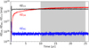 |
Fig. A.1. Temporal evolution of the volume-integrated kinetic energies. Shown are the kinetic energy of the differential rotation KEDR (red), the kinetic energy of the meridional circulation KEMC (blue), and the kinetic energy of the nonaxisymmetric flows KECV (black). The results from the six runs starting with different initial conditions are shown. The gray shaded area denotes the duration used for our spectral analysis. |
Appendix B: Effective turbulent diffusivity
In this appendix we give an estimate of the effective turbulent diffusivity in our nonlinear simulation νeff due to the small-scale convective motions on resolved scales. Using the first-order smoothing approximation (FOSA) (e.g., Moffatt 1978), we calculate νeff as
 (B.1)
(B.1)
where the convective turnover timescale τc is given by Hp/vrms. Here the rms convective velocity is calculated at each height as
 (B.2)
(B.2)
Figure B.1c shows that νeff is about 3 × 1012 cm2 s−1 throughout the convection zone. This value is comparable but slightly higher than the explicit viscosity value of ν = 1012 cm2 s−1, which we use in the simulation. This implies that the turbulent convective motions can have an impact on inertial modes by enhancing the effective viscous diffusivity. Still, this enhanced value is lower than the value estimated using a mixing-length model (Muñoz-Jaramillo et al. 2011).
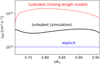 |
Fig. B.1. Radial profiles of the effective diffusivity due to small-scale convective motions νeff (black solid line). For comparison, the explicit viscosity used in the simulation and the turbulent diffusivity estimated based on the mixing-length model (Muñoz-Jaramillo et al. 2011) are also shown (blue and red dashed lines). |
Appendix C: High-latitude inertial modes
Bekki et al. (2022) reported that there are retrograde-propagating z-vorticity modes that are predominantly confined inside the tangential cylinder. They are called “topographic” Rossby modes because they originate from the topographic β-effect, the spherical curvature effect of the lower and upper boundaries. When seen at the surface, these modes are found only at high latitudes, and thus are also called “high-latitude” modes (Gizon et al. 2021).
In this appendix we show that the high-latitude modes, as well as the equatorial modes, can be unambiguously identified in our nonlinear rotating convection simulation. We find that they exist predominantly at m = 1. For m = 2 and 3 the power still exists, but it is substantially weaker. Figure C.1a shows the m = 1 power spectrum of the north-south antisymmetric component of vθ as a function of latitude at the base of the convection zone r = 0.71R⊙. The power of the high-latitude mode can be seen at ω/2π ≈ −105 nHz from middle to high latitudes. The extracted eigenfunctions of this m = 1 mode are shown in the lower panels of Fig. C.1b and are compared with the results of linear analysis (upper panels). The associated flow is dominantly z-vortical and is strongly confined inside the tangential cylinder. The z-vorticity ζz is north-south symmetric across the equator. The product of ζz and p1 is negative throughout the domain, suggesting that the mode is in geostrophic balance.
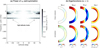 |
Fig. C.1. High-latitude inertial mode with north-south symmetric ζz. (a) Power spectrum of the north-south antisymmetric component of latitudinal velocity vθ at the base of the convection zone r = 0.71R⊙ for m = 1 as a function of latitude. The power associated with the high-latitude mode is denoted by black arrows at ω/2π ≈ −105 nHz. (b) Extracted eigenfunctions of the m = 1 mode. The lower and upper panels show the eigenfunctions extracted from the simulation and from the linear analysis, respectively. |
In addition to the ζz-symmetric mode, we also identify the north-south ζz-antisymmetric high-latitude mode in our simulation. Figure C.2a shows the same power spectrum as Fig. C.1a, but for the symmetric component of vθ between the hemispheres. The power of the high-latitude mode lies at ω/2π ≈ −48 nHz at latitudes above ±50°, whereas the n = 0 equatorial Rossby mode is spotted at ω/2π ≈ −395 nHz at low latitudes. Figure C.2b shows the extracted eigenfunctions of ζz-antisymmetric high-latitude mode at m = 1. Unlike the symmetric mode, ζz is dissected between the hemispheres. However, a latitudinal velocity exists at the equator, which can correlate the vortices between the hemispheres.
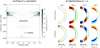 |
Fig. C.2. High-latitude inertial mode with north-south antisymmetric ζz. (a) Power spectrum of the north-south symmetric component of vθ at the base of the convection zone r = 0.71R⊙ at m = 1 as a function of latitude. The high-latitude mode’s power exists at a frequency of about −48 nHz, whereas the power of the n = 0 equatorial Rossby mode can be seen at ω/2π ≈ −395 nHz. (b) Same as Fig. C.1b, but for the mode with north-south antisymmetric ζz. |
The horizontal velocity amplitudes of these high-latitude modes are 1 − 2 m s−1 at m = 1 (regardless of the north-south symmetries). As Bekki et al. (2022) reported, when the latitudinal entropy variation is significant throughout the convection zone, these modes become baroclinically unstable and exhibit a spiralling pattern around the poles, as observed on the Sun (Hathaway & Upton 2021; Gizon et al. 2021). However, in the simulation reported here the latitudinal entropy variation is too weak for the baroclinic instability to occur. Therefore, the observed spiralling features are not reproduced.
All Tables
All Figures
|
Fig. 1. Yin-Yang grid used in our simulation. (a) Three-dimensional view of the Yin and Yang grids. The blue and red lines show the Yin and Yang coordinates, respectively. (b) Mollweide projection of the Yin-Yang grid. The thick black curve denotes the location where the horizontal boundary condition is set in our code. |
| In the text | |
|
Fig. 2. Temporally averaged profile of (a) the differential rotation Ω(r, θ)=Ω0 + ⟨vϕ⟩/rsinθ, and (b) the streamlines of the meridional circulation vm = (⟨vr⟩,⟨vθ⟩). Here ⟨⟩ denotes the longitudinal average. The meridional flow stream function Ψ is defined by ρ0vm = ∇ × (Ψeϕ). Red (blue) indicates the circulation is clockwise (counter-clockwise), i.e., the flow is poleward (equatorward) near the surface at high latitudes in both hemispheres. |
| In the text | |
|
Fig. 3. Snapshots of the convective pattern in our simulation near the top boundary r = 0.95R⊙. Panels a and b: radial velocity vr and nonaxisymmetric component of the longitudinal velocity vϕ. |
| In the text | |
|
Fig. 4. Equatorial power spectra of longitudinal velocity vϕ. (a) The power spectrum near the top boundary r = 0.95 R⊙. The power is normalized at each m. The spectrum is computed in a frame rotating at Ω0/2π = 431.3 nHz (the rotation rate of the radiative interior). The blue line represents the advective speed by the local differential rotation, m[Ω(0.95R⊙,π/2)−Ω0]. Overplotted in red is the dispersion relation of the columnar convective modes from the linear eigenmode calculation. (b) Same equatorial power spectrum as in (a), but at fixed azimuthal order m = 8 as a function of depth. The blue line is again the local advection frequency and the red line is the eigenfrequency from the linear analysis. |
| In the text | |
|
Fig. 5. Three-dimensional visualization of the columnar convective modes. Left: snapshot of pressure perturbation (nonaxisymmetric component) from the nonlinear simulation shown as a 3D volume rendering. The red-yellow and blue-cyan parts correspond to the regions with positive and negative pressure perturbations, respectively. Right: eigenfunctions of pressure perturbation of the columnar convective modes extracted from the simulation data using SVD. The cases with m = 2 and m = 12 are shown. |
| In the text | |
|
Fig. 6. Spatial eigenfunctions qα, mode(r, θ, m) for the ζz-symmetric columnar convective modes with m = 2. By definition, modes are of the form qα, mode(r, θ, m)exp[i(mϕ−ωt)], where qα is either vr, vθ, vϕ, or p1. (a) Meridional cuts of the radial velocity vr, latitudinal velocity vθ, longitudinal velocity vϕ, and pressure perturbation p1 extracted from the convection simulation (lower panels) and obtained from our linear calculation (upper panels). (b) Radial dependence of the eigenfunction vϕ at the equator. The black solid and red dashed lines represent the simulation and linear calculation, respectively. (c) Latitudinal eigenfunction of vϕ at the surface normalized near the equator. |
| In the text | |
|
Fig. 7. Power spectra of latitudinal velocity vθ near the equator (averaged over ±15 deg). Panels a and b: m − ω diagram near the base (r = 0.75 R⊙) and near the surface (r = 0.95 R⊙), respectively. The power is normalized at each m. The spectra are computed in a frame rotating at Ω0/2π = 431.3 nHz. Overplotted in red line in panel a is the dispersion relation of the equatorial Rossby mode with no radial node (n = 0) obtained from the linear calculation. The blue line represents the advection frequency of the equatorial differential rotation, m[Ω(r,π/2)−Ω0], at each height. Panels c and d: power spectra at fixed azimuthal order m = 1 and m = 16, respectively. |
| In the text | |
|
Fig. 8. Eigenfunctions of the equatorial Rossby mode with no radial node (n = 0) for m = 2. (a) Meridional eigenfunctions extracted from the simulation (lower panels) and those obtained from the linear analysis (upper panels). The same notation is used as in Fig. 6a. (b) Radial eigenfunction of vθ at the equator. The black solid and red dashed lines show the results from the simulation and linear calculation, respectively. (c) Latitudinal eigenfunction of vθ in the middle convection zone. |
| In the text | |
|
Fig. 9. Extracted eigenfunctions of the n = 0 equatorial Rossby modes at m = 24. Eigenfunctions of radial velocity (imaginary) ℑ[vr], latitudinal velocity (real) ℜ[vθ] and (imaginary) ℑ[vθ], longitudinal velocity (real) ℜ[vϕ], pressure perturbation (real) ℜ[p1], and entropy perturbation (imaginary) ℑ[s1] are shown from left to right. The real and imaginary phases are determined in a way such that ℜ[vθ] at the base takes its maximum at the equator. |
| In the text | |
|
Fig. 10. Radial structure of the real eigenfunctions of latitudinal velocity ℜ[vθ] at the equator. The eigenfunctions are normalized to unity at the base. The different colors represent different azimuthal orders m (see inset). The solid and dashed lines denote the eigenfunctions extracted from the nonlinear simulation and from the linear eigenmode calculation, respectively. |
| In the text | |
|
Fig. 11. Schematic illustration of the flow structure of the n = 0 equatorial Rossby modes at (a) low-m and (b) high-m regimes. |
| In the text | |
|
Fig. 12. Power spectra of horizontal velocities near the surface extended to negative azimuthal orders (m < 0). (a) Equatorial power spectrum of north-south symmetric component of vθ near the top boundary r = 0.95 R⊙, which is the same as Fig. 7b. The power is normalized at each m. Shown in red points are the frequencies of the mixed Rossby modes obtained from our linear analysis. The blue line represents the advection frequency of the equatorial differential rotation, m[Ω(0.95 R⊙,π/2)−Ω0]. (b) Equatorial power spectrum of north-south antisymmetric component of vϕ near the top boundary r = 0.95 R⊙. |
| In the text | |
|
Fig. 13. Eigenfunctions of the retrograde-propagating mixed Rossby mode (n = 1 equatorial Rossby mode). (a) Meridional cuts of the eigenfunctions at m = 2. The lower and upper panels respectively show the results extracted from the simulation and from the linear analysis. (b) Schematic illustration of this mode. |
| In the text | |
|
Fig. 14. Eigenfunctions of the prograde-propagating mixed Rossby mode (north-south ζz-antisymmetric columnar convective mode). (a) Meridional cuts of the eigenfunctions at m = 2. Lower and upper panels: respectively show the results extracted from the simulation and from the linear analysis. (b) Schematic illustration of this mode. |
| In the text | |
|
Fig. 15. Spectra of the equatorial modes. (a) Maximum horizontal velocity vh of the equatorial modes near the top boundary r = 0.95 R⊙ at each azimuthal order m. The red, blue, and green points represent the ζz-symmetric columnar convective modes, n = 0 equatorial Rossby modes, and the mixed Rossby modes, respectively. The black dashed line represents the overall power of the convection simulation (including modes at high latitudes and stochastic convective motions). The cyan diamonds and squares denote the (rms) horizontal velocity amplitudes of the observed Rossby modes near the solar surface obtained by Liang et al. (2019) and Gizon et al. (2021), respectively. (b) Spectra of the volume-integrated kinetic energy of the equatorial modes. |
| In the text | |
|
Fig. 16. Enthalpy fluxes Fe associated with the extracted modes in our simulations summed over m = 1 − 39. Panels a–c: ζz-symmetric columnar convective modes, the n = 0 equatorial Rossby modes, and the mixed Rossby modes, respectively. Panel d: the total enthalpy flux (including other modes and small-scale convection) is shown. The fluxes are normalized by the injected energy flux F* = L*/(4πr2). |
| In the text | |
|
Fig. 17. Reynolds stresses associated with the extracted modes in our simulations summed over m = 1 − 39. Panels a–c: ζz-symmetric columnar convective modes, the n = 0 equatorial Rossby modes, and the mixed Rossby modes, respectively. Panel d: the total Reynolds stresses (including other modes and small-scale convection) is shown. Upper and lower panel: respectively corresponds to ρ0⟨vrvϕ⟩ and ρ0⟨vθvϕ⟩. |
| In the text | |
|
Fig. A.1. Temporal evolution of the volume-integrated kinetic energies. Shown are the kinetic energy of the differential rotation KEDR (red), the kinetic energy of the meridional circulation KEMC (blue), and the kinetic energy of the nonaxisymmetric flows KECV (black). The results from the six runs starting with different initial conditions are shown. The gray shaded area denotes the duration used for our spectral analysis. |
| In the text | |
|
Fig. B.1. Radial profiles of the effective diffusivity due to small-scale convective motions νeff (black solid line). For comparison, the explicit viscosity used in the simulation and the turbulent diffusivity estimated based on the mixing-length model (Muñoz-Jaramillo et al. 2011) are also shown (blue and red dashed lines). |
| In the text | |
|
Fig. C.1. High-latitude inertial mode with north-south symmetric ζz. (a) Power spectrum of the north-south antisymmetric component of latitudinal velocity vθ at the base of the convection zone r = 0.71R⊙ for m = 1 as a function of latitude. The power associated with the high-latitude mode is denoted by black arrows at ω/2π ≈ −105 nHz. (b) Extracted eigenfunctions of the m = 1 mode. The lower and upper panels show the eigenfunctions extracted from the simulation and from the linear analysis, respectively. |
| In the text | |
|
Fig. C.2. High-latitude inertial mode with north-south antisymmetric ζz. (a) Power spectrum of the north-south symmetric component of vθ at the base of the convection zone r = 0.71R⊙ at m = 1 as a function of latitude. The high-latitude mode’s power exists at a frequency of about −48 nHz, whereas the power of the n = 0 equatorial Rossby mode can be seen at ω/2π ≈ −395 nHz. (b) Same as Fig. C.1b, but for the mode with north-south antisymmetric ζz. |
| In the text | |
Current usage metrics show cumulative count of Article Views (full-text article views including HTML views, PDF and ePub downloads, according to the available data) and Abstracts Views on Vision4Press platform.
Data correspond to usage on the plateform after 2015. The current usage metrics is available 48-96 hours after online publication and is updated daily on week days.
Initial download of the metrics may take a while.