© The Authors 2025

1. Introduction

Rossby and inertial modes of solar oscillation are observed in long-duration time series of the horizontal velocity field on or near the solar surface (Löptien et al. 2018; Gizon et al. 2021; Hanson et al. 2022). These horizontal flows may be inferred at a daily cadence using local helioseismology applied to the Global Oscillation Network Group (GONG: Harvey et al. 1996) and the Helioseismic and Magnetic Imager onboard the Solar Dynamics Observatory (SDO/HMI: Scherrer et al. 2012) data sets, or using local correlation tracking of granulation (seen in SDO/HMI intensity images). The observed modes have periods on the order of the solar rotation period and their surface eigenfunctions are quasi-toroidal. Linear eigenvalue solvers enable us to identify the various modes that are clearly resolved in frequency space and to infer their radial eigenfunctions throughout the convection zone (Bekki et al. 2022). The equatorial Rossby modes have maximum colatitudinal velocity, v_θ, at the equator, while the high-latitude modes have maximum longitudinal velocity, v_ϕ, in the polar regions. Nearly all modes have critical latitudes where their phase speeds equal the local differential rotation velocity. In the observations, the inertial modes are unambiguously identified as global modes because each mode oscillates at the same frequency over a large range of latitudes (Gizon et al. 2021). Waidele & Zhao (2023) and Lekshmi et al. (2024) measure the temporal variations of the equatorial Rossby mode properties using the horizontal flows from helioseismic analysis of HMI and GONG data, and report that the mode power (frequency shift) averaged over azimuthal wavenumber m is correlated (anticorrelated) with the sunspot cycle. We refer the reader to Gizon et al. (2024) for a review on the topic of solar inertial modes.

The high-latitude inertial mode with m = 1 (hereafter HL1 for short) is of particular interest. It has the largest amplitude among all modes in the inertial frequency range (time-averaged v_ϕ ∼ 10 m/s, see Gizon et al. 2021) and it is driven by a baroclinic instability (Bekki et al. 2022). This mode is very sensitive to the latitudinal entropy gradient and to other important properties of the solar convection zone, such as the superadiabatic temperature gradient (Gizon et al. 2021; Bekki et al. 2022, 2024). The mode is anti-symmetric across the equator in v_ϕ and symmetric in v_θ. Its mean frequency over the period 2010–2020 is measured to be ${\nu }_{HL1}^{\mathrm{Carr}}=-86.3\pm 1.6$ nHz in the Carrington frame, where the negative sign indicates retrograde propagation. In an inertial frame, the sidereal frequency is

$$\begin{array}{c}\hfill {\nu }_{HL1}=-86.3+456.0\mathrm{nHz}=369.7\mathrm{nHz}\end{array}$$(1)

and in the Earth frame the synodic frequency is

$$\begin{array}{c}\hfill {\nu }_{HL1}^{\mathrm{synodic}}=369.7-31.7\mathrm{nHz}=338.0\mathrm{nHz}.\end{array}$$(2)

Above 50° latitude, the mode has a characteristic spiral pattern in v_ϕ, which, according to models, depends sensitively on the properties of the convection zone (Gizon et al. 2021). The flow pattern associated with the m = 1 mode was first reported by Hathaway et al. (2013) using a supergranulation tracking method, although it was then misidentified as giant cell convection sheared by differential rotation. Bogart et al. (2015) later confirmed the existence of the m = 1 polar flow pattern using ring-diagram analysis.

It came to our attention only recently that the m = 1 high-latitude inertial mode of oscillation was clearly seen above 50° latitude in the “zonal velocity” time series computed from Mt. Wilson Observatory (MWO) Dopplergrams by Ulrich (1993, his Figure 5, top panel) and Ulrich (2001, his Figure 1, top panel). Ulrich et al. (1988) defined the zonal velocity as

$$\begin{array}{c}\hfill V_{\mathrm{zonal}}(\theta )=\frac{{\displaystyle {\sum }_{|L|<30°}}(sinL)[V_{\mathrm{los}}(\theta ,L)-V_{\mathrm{background}}(\theta ,L)]}{{\displaystyle {\sum }_{|L|<30°}}|sinL|},\end{array}$$(3)

where V_los is a Dopplergram and V_background is the Doppler image consisting of the limb shift plus the line-of-sight (LOS) projection of the Sun’s axisymmetric flows (rotation and meridional circulation). The co-latitude is denoted by θ and L = ϕ − ϕ_c is the heliographic longitude measured with respect to the central meridian ϕ_c. The zonal velocity informs us about the slowly-varying large-scale components of the longitudinal velocity v_ϕ on the Sun. The velocity V_zonal can be used to measure the “torsional oscillation”, and also to detect the inertial modes.

In Figure 4 of Ulrich (2001), the m = 1 high-latitude mode is visible in V_zonal at latitudes ±58.5° as narrow peaks of power with very high signal-to-noise ratio at a sidereal frequency close to 0.8 × (CarringtonPeriod)⁻¹ = 0.8 × 456 nHz = 365 nHz. This frequency corresponds to ν_HL1 given in Eq. (1) and is slightly above the local rotation rate. At the lower latitudes (below 40°), other peaks of excess power are seen at frequencies that follow the local frequency of the surface differential rotation (increases toward the equator); these peaks are unrelated to the HL1 mode, but are likely due to velocity features that are associated with magnetic activity advected at the local rotation rate.

In the present paper, we use all three available series of full-disk Dopplergrams (MWO, GONG, and HMI) to study the long-term evolution of the HL1 mode. We find that the mode is visible in V_zonal in the latitude range 60° – 75° throughout the entire period from 1967 to 2024. We characterize the evolution of the HL1 mode parameters and study their correlations with the sunspot number, the polar field strength, and the solar rotation rate. The steps to obtain the HL1 mode parameters are detailed in Sections 2, 3, and 5, and summarized in Fig. 1. We note that preliminary results using only GONG and HMI were presented by Gizon et al. (2024).

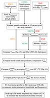Fig. 1. Schematics of data processing steps involved in the measurement of the velocity amplitude of the HL1 mode from MWO, GONG, and HMI time series of Dopplergrams.

2. Detection of HL1 mode in MWO, GONG, and HMI Dopplergrams

The time periods used in the analysis are from 1967 to 2012 for MWO data, from 2001 to 2024 for GONG data (tdvzi), and from 2010 to 2024 for HMI data (hmi.v_720s). The original time cadences and spatial resolutions of the data sets are quite different. For the purpose of this work, we took one frame per day and reduced the resolution to 10″per pixel by binning.

2.1. Correction of GONG and HMI Dopplergrams

The static limb shift, differential rotation, and meridional circulation velocity signals were already subtracted from the MWO data by Ulrich (2001), thus no V_background subtraction is necessary for this dataset. For the other two datasets, we perform low-order polynomial fits to V_los to obtain V_background. For the limb shift, we fit a model that consists of a polynomial of order five in μ, where μ is the cosine of the center-to-limb angle. For the LOS projection of the trends in the east-west and north-south directions, we fit the following models:

$$\begin{array}{cc}\hfill V_{\mathrm{los}}^{(\mathrm{EW})}(\theta ,L)& =cos{B}_{0}sin\theta sinL{\displaystyle \sum _{k=0}^4}{b}_k{(cos\theta )}^k,\hfill \end{array}$$(4)

$$\begin{array}{cc}\hfill V_{\mathrm{los}}^{(\mathrm{NS})}(\theta ,L)& =(sin{B}_{0}sin\theta -cos{B}_{0}cos\theta cosL){\displaystyle \sum _{l=1}^4}{c}_l{P}_l^1(cos\theta ),\hfill \end{array}$$(5)

where B₀ is the heliographic latitude at the disk center and the P_l¹ are associated Legendre polynomials of degree l and order one. The model parameters are estimated using a least-squares method. We correct the V_los by subtracting daily fits to the limb shift and $V_{\mathrm{los}}^{(\mathrm{NS})}$. For $V_{\mathrm{los}}^{(\mathrm{EW})}$, however, we subtract a long-term average instead, in order to preserve the zonal velocity component of low-m inertial modes in V_los. We note that we apply the procedure to the unmerged GONG data (tdvzi), because the merged GONG data (mrvzi) are affected by the removal of a surface fit to the data, which undesirably reduces the amplitude of the low-m modes.

The HMI Doppler time series also contains a number of jumps, which coincide with the re-tuning of the optical filter system (Couvidat et al. 2016; Hoeksema et al. 2018). This affects the interference fringes. In the hmi.v_720s data series, the fringes were largely removed from 1 October 2012 onward (see Couvidat et al. 2016, their Section 2.8.2 and their Figures 9 and 10). However the fine structure of the fringes still remains in this data set (see Fig. A.1). To remove the HMI fringes, we subtract the median values of the images computed over time intervals between adjacent re-tuning dates.

2.2. Computation of zonal velocity

In order to compute the zonal velocity for MWO, GONG, and HMI using Eq. (3), we remap the corrected Dopplergrams onto heliographic coordinates using the equidistant cylindrical projection with a map scale of 0.6° per pixel, to obtain (V_los − V_background) as a function θ, L, and time. We choose to sum over longitudes |L|< 30° and average over nine consecutive days, in order to follow the procedure described by Ulrich et al. (1988). The resulting time series of zonal velocity, V_zonal(θ, t), are kept in the Earth frame.

2.3. Visual detection of HL1 mode in supersynoptic maps

To enhance the visibility of the HL1 mode in V_zonal, we apply a high-pass temporal filter to remove the slow variations below 200 nHz, including the torsional oscillation and the B₀-angle periodicities. Figure A.2 shows all the supersynoptic maps of V_zonal as functions of time and latitude for the three data sets (MWO, GONG, HMI). The black and white stripes at high latitudes correspond to the HL1 inertial mode. Importantly, these stripes are consistent between the overlapping data sets (see arrows in Fig. A.2). Figure 2 shows selected time periods from Fig. A.2 showing only five years of data around each solar cycle minimum. The mode amplitude is strongest during these quiet Sun periods.

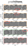Fig. 2. Example supersynoptic maps of Vzonal in the Earth frame computed from the MWO (top three panels), GONG (fourth panel), and HMI data (bottom panel) near cycle minima. The full data set is shown in Fig. A.2). The HL1 mode may be seen from time to time as stripes in Vzonal above 50° latitude (see regions in red ellipses). For clarity, the maps were smoothed in latitude with a Gaussian kernel of width 10°.

2.4. Consistency between datasets during overlapping time periods

Since the global mode HL1 is antisymmetric across the equator in V_zonal, we compute the north-south antisymmetric zonal velocity $V_{\mathrm{zonal}}^{(-)}(\theta ,t)=[V_{\mathrm{zonal}}(\theta ,t)-V_{\mathrm{zonal}}(\pi -\theta ,t)]/2$ to reduce noise. We then compute an average of $V_{\mathrm{zonal}}^{(-)}$ over the latitudinal range 60°–75° where the mode is easily detectable:

$$\begin{array}{c}\hfill V_{\mathrm{zonal}}^{(\mathrm{band})}(t)={\langle V_{\mathrm{zonal}}^{(-)}(\theta ,t)\rangle }_{|\theta -22.5^{°}|\le 7.5^{°}}.\end{array}$$(6)

Figure 3 shows extracts from $V_{\mathrm{zonal}}^{(\mathrm{band})}$ for overlapping time segments between MWO, GONG, and HMI. The consistency between the overlapping data sets is clear.

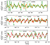Fig. 3. $V_{\mathrm{zonal}}^{(\mathrm{band})}(t)$ during different overlapping periods of the MWO, GONG, and HMI data. The period of the predominant oscillations seen in $V_{\mathrm{zonal}}^{(\mathrm{band})}$ is about 34 days, which corresponds to the HL1 mode frequency near ${\nu }_{HL1}^{\mathrm{synodic}}=338$ nHz.

3. Power spectra of zonal velocity

We then Fourier transform each of the MWO, GONG, and HMI $V_{\mathrm{zonal}}^{(\mathrm{band})}(t)$ to obtain three power spectra,

$$\begin{array}{c}\hfill P(\nu )=\frac{1}{\mathrm{\Delta }\nu N_t^2\eta }{\left|{\displaystyle \sum _t}{V}_{\mathrm{zonal}}^{(\mathrm{band})}(t)e^{-2\pi \mathrm{i}\nu t}\right|}^2,\end{array}$$(7)

where N_t = 16824 for MWO, N_t = 8462 for GONG, N_t = 5267 for HMI, with a common temporal sampling Δt = 1 day. The quantity Δν = 1/(N_tΔt) is the frequency resolution, equal to 0.7 nHz for MWO, 1.4 nHz for GONG, and 2.2 nHz for HMI. To correct for missing data, we divide the power by the duty cycle η = 0.96 for MWO, η = 0.96 for GONG, and η = 1 for HMI.

Figure 4 shows P(ν) for the full time series of the three data sets. In all cases, excess power is detected around the reference HL1 mode frequency ${\nu }_{HL1}^{\mathrm{synodic}}=338$ nHz. The mode power differs between the three data sets. This is not because of varying data quality, but because they do not cover the same time periods. We shall confirm later that the mode power and frequencies measured from the three data sets are consistent during their overlap periods. The central frequency of the peak in the HMI P(ν) is 2 nHz off from the reference ${\nu }_{HL1}^{\mathrm{synodic}}$, although the reference frequency was obtained using the HMI data in a similar time period. One possible explanation is that Gizon et al. (2021) obtained the HL1 mode frequency using the latitude range 37.5°–67.5° where the excess power around the local differential rotation rate (highlighted by the blue curves in their Figure 1) remains significant and thus the measured frequency was slightly biased.

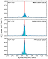Fig. 4. Power spectra of $V_{\mathrm{zonal}}^{(\mathrm{band})}$ in the frequency range 250–450 nHz (in the Earth frame), computed from the MWO, GONG, and HMI Dopplergrams (from top to bottom respectively). The vertical red lines at 338 nHz mark the reference synodic frequency of the HL1 mode.

In all three data sets the background noise level is extremely low. The full width of the peak is approximately w = 4 ∼ 6 nHz. This corresponds to an e-folding lifetime of 1/(πw)∼2 years.

As will be seen later in the three-year power spectra of Fig. 6 (middle column), the mode is continuously visible since 1969.

4. Velocity pattern associated with the HL1 mode

Let us infer the LOS velocity perturbation associated with the HL1 mode from the series of Dopplergrams. We align the disk centers of the HMI V_los images, rotate the images by the nominal roll angle provided by the HMI team (−CROTA2), and re-scale the disk radius to a common value. Instead of taking one frame per day, we compute daily averages of the images to reduce the noise. At each pixel (x, y) on the disk, we apply a band-pass filter to the data in the Fourier domain centered around the synodic mode frequency to obtain

$$\begin{array}{c}\hfill V_{\mathrm{los}}^{HL1}(x,y,t):=\frac{1}{N_t}{\displaystyle \sum _{\nu }}\mathrm{filt}\left(\frac{\nu -338\mathrm{nHz}}{75\mathrm{nHz}}\right){\widehat{V}}_{\mathrm{los}}(x,y,\nu )e^{2\pi \mathrm{i}\nu t},\end{array}$$(8)

where filt(ξ) is a symmetric function equal to 1 for |ξ|< 1/3, tapered to zero with raised cosines, and with a full width at half maximum of 1. In the above expression, ${\widehat{V}}_{\mathrm{los}}$ denotes the temporal FFT of V_los.

Figure 5 shows an example of a filtered Dopplergram during the solar minimum in 2018, at a time when the north pole is tilted toward the Earth. The image was smoothed using a 2D Gaussian kernel with a FWHM of 5° to reduce noise on small spatial scales. The horizontal velocity of the HL1 mode projected onto the line of sight is clearly seen above 50° latitude in both hemispheres. Notice that there appears to be a polar-crossing flow with an amplitude over 10 m/s associated with the HL1 mode (in agreement with an early statement by Ulrich 1993, page 35). In the left column of Fig. A.3, we can see the line-of-sight projection of the mode velocity at different times (different phases) with different B₀ angles. The predominant pattern in $V_{\mathrm{los}}^{HL1}$ at high latitudes is mostly north-south antisymmetric.

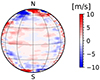Fig. 5. Line-of-sight Doppler velocity associated with the HL1 mode as viewed from the Earth on 09 September 2018 when the solar tilt angle B0 is 7.24°, extracted from time series of daily HMI images by applying a band-pass filter around ${\nu }_{HL1}^{\mathrm{synodic}}$ (see Eq. (8)). The LOS velocity pattern in the polar regions is associated with the HL1 mode. The image was smoothed using a 2D Gaussian kernel with a FWHM of 5°. A comparison with the reconstructed $V_{\mathrm{los}}^{HL1}$ using 5°-tile ring-diagram flow maps is shown in Fig. A.3 and in the online movie.

To compare with the Doppler data, we also reconstruct $V_{\mathrm{los}}^{HL1}$ using the 5°-tile horizontal flow maps near the solar surface from the HMI ring-diagram pipeline (Bogart et al. 2011a,b). Because the ring-diagram flow maps (V_Carr) are given in the Carrington frame, it is necessary to apply at each position vector r (defined from the center of the Sun) the following velocity transformation from the Carrington frame to the Earth frame,

$$\begin{array}{c}\hfill {\mathit{V}}_{\oplus }={\mathit{V}}_{\mathrm{Carr}}+({\mathrm{\Omega }}_{\mathrm{Carr}}{\mathit{z}}_{\odot }-{\mathrm{\Omega }}_{\oplus }\mathit{z})\times \mathit{r},\end{array}$$(9)

where Ω_Carr/2π = 456 nHz is the Carrington rotation rate, z_⊙ is the unit vector that points along the solar rotation axis, Ω_⊕/2π = (1 yr)⁻¹ = 31.7 nHz, and z is the unit vector that points along the normal to the ecliptic plane. The second term on the right-hand side of Eq. (9) does not affect the frequencies within the HL1 band-pass filter. Thus the $V_{\mathrm{los}}^{HL1}$ reconstructed from the ring-diagram flow maps is essentially V_Carr projected onto the line of sight, followed by the HL1 mode filtering.

The middle column of Fig. A.3 shows the reconstructed $V_{\mathrm{los}}^{HL1}$ from the ring-diagram flow maps, to be compared with $V_{\mathrm{los}}^{HL1}$ maps from the direct Doppler. The large-scale patterns and the velocity amplitudes are in very good agreement between the two data sets, especially at high latitudes. This suggests in particular that the HL1 mode does not have any significant radial motion (since we did not consider this component in the reconstruction of the Doppler data). At lower latitudes, the large-scale features have much lower amplitudes but also agree. A movie showing the evolution of $V_{\mathrm{los}}^{HL1}(x,\mathit{y},t)$ and its ring-diagram reconstruction at a cadence of 1 day during 2010–2022 is available online. At high latitudes, the agreement is good between the two data sets, although noise is higher in the ring-diagram data set. This is not too surprising as we expect helioseismic analysis to contain stochastic p-mode noise that is not present in Doppler data at a daily temporal cadence.

Let us study the random noise in $V_{\mathrm{los}}^{HL1}$ in more detail. We estimate the noise level by subtracting from $V_{\mathrm{los}}^{HL1}$ a spatial smoothing with a Gaussian FWHM of 15° and computing the rms of the residuals in time for each pixel. As shown in Fig. A.3 (bottom row), the rms noise level in direct $V_{\mathrm{los}}^{HL1}$ is below 2 m/s, with a minimum of 0.2 m/s near disk center. The noise level increases with disk radius because an angular distance of 5° corresponds to about 8 pixels near the disk center but only about one pixel near the limb. The noise level in the reconstructed data from ring-diagram flow maps is also around 0.2 m/s near disk center, but it increases much faster with disk radius than that in the direct Doppler data. We also note that the reconstructed images from helioseismology are only available up to 98% of the disk radius. On the other hand, the Dopplergrams cover the entire solar disk, which is much useful to observe the high-latitude HL1 mode.

In the right column of Fig. A.3 we also compare the observations with the line-of-sight projection of the theoretical velocity eigenfunction (Gizon et al. 2021; Bekki et al. 2022). We find a reasonable agreement; however, there are also noticeable differences between observations and theory. In particular the tilt of the velocity pattern changes faster with latitude in the observations than in theory.

We remark that the tilt of the spiral pattern at high latitudes in Fig. 5 is in the opposite direction to that of Fig. 2, since in the supersynoptic maps the corresponding longitude decreases toward the right along the horizontal axis. We also note that we avoided performing spatial Fourier transform, since we do not see the entire solar surface and LOS projection effects may complicate the interpretation of the spatial power spectra.

5. Evolution of HL1 mode parameters

5.1. Power spectra from three-year data segments

We break down the time series into three-year segments to extract the HL1 mode parameters as a function of time. We use the MWO data from 1969 to 2010 and the HMI data from 2011 to 2022, giving a total of 18 non-overlapping segments covering five solar cycles.

We compute the power spectra for each of these three-year segments. Above 45° latitude, the mode is detected in all data sets as narrow peaks of power near synodic frequency 338 nHz well above noise level. This can be seen for two example time segments in Fig. 6 (panels b and d). Below 45°, the mode is in the noise in the MWO data (Fig. 6b), while it remains visible below in the HMI power spectra (Fig. 6d). We note that there is also some excess power at frequencies corresponding to the local differential rotation (highlighted by the shaded pink areas), indicating that some velocity features are advected by the local rotation, such as flows around active regions (Gizon 2004), convective flows, or possibly critical-latitude modes (Gizon et al. 2021; Fournier et al. 2022). The background power drops to zero below 200 nHz since we applied a high-pass filter to the time series of V_zonal to remove long-term trends including the torsional oscillation and B₀-angle variation.

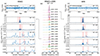Fig. 6. Visibility of HL1 mode in consecutive three-year power spectra, using MWO (1969–2010) and HMI (2011–2022) data. Panel a: example MWO time series (1984–1986) of $V_{\mathrm{zonal}}^{(-)}$ averaged over latitudes 60° ≤λ < 75° (i.e., $V_{\mathrm{zonal}}^{(\mathrm{band})}$). Panel b: power spectra of $V_{\mathrm{zonal}}^{(-)}$ for the same time period in various latitudinal bands of 15° (labeled at the top right corner of each panel). The vertical red lines denote the reference HL1 mode frequency ${\nu }_{HL1}^{\mathrm{synodic}}=338$ nHz and the excess power around this frequency is highlighted in blue. The shaded pink areas indicate the differential rotation rate in the outer 5% of the Sun from global helioseismology as viewed from the Earth. Panels c and d: same as above but for an example HMI three-year time series during 2017–2019. Panel e: all available three-year power spectra of $V_{\mathrm{zonal}}^{(\mathrm{band})}$ stacked on top of each other. The crosses highlight the reference frequency of 338 nHz.

The middle column of Fig. 6 shows the 3-year power spectra above 60° latitude, stacked on top of each other in the (synodic) frequency range 250–450 nHz. The HL1 mode power is always present, although it is smaller during the periods 1972–1974 and 1993–1995. We see that the noise level in the MWO data improved from 1982 when a new exit slit assembly was installed, and from 1986 when the fast scan program started, as reported by Ulrich et al. (1988). We find that it is possible to follow the evolution of the mode amplitude over the full extent of the data sets (MWO, GONG, HMI) with a time resolution of at least three years. It is remarkable that the MWO data enable us to add three decades of very useful observations.

5.2. Estimation of mode parameters

To improve the temporal sampling, we now consider sliding time windows of three years with central times separated by one year, such that each time window has an overlap of two years with the neighboring windows. To extract the HL1 mode parameters in each time window, we choose to fit a Lorentzian function to the corresponding power spectra,

$$\begin{array}{c}\hfill L(\nu )=\frac{A}{1+{[(\nu -{\nu }_{HL1}+31.7\mathrm{nHz})/(w/2)]}^2}+B,\end{array}$$(10)

where ν_HL1 is the sidereal mode frequency, A is the mode power, w is the full width at half maximum of the Lorentzian, and B the constant background over the fitting range 200–500 nHz. The total power of the HL1 mode under the Lorentzian profile is πAw. The rms and maximum values of the mode velocity amplitude ($V_{\mathrm{zonal}}^{(\mathrm{band})}$) are given by $\sqrt{\pi Aw}$ and $\sqrt{2\pi Aw}$ respectively.

We note that we padded each 3-yr time segment of $V_{\mathrm{zonal}}^{(\mathrm{band})}$ with zeros to have a length of N_t = 8192 and a frequency resolution of Δν = 1.4 nHz. The original frequency resolution from a 3-yr time segment (10.6 nHz) is coarser than the line width of the HL1 mode (4–6 nHz; see Sect. 3), making it tricky to fit. The mode power πAw is unaffected by the zero padding as the duty cycle η has taken this into account in Eq. (7); however, the line profile is broadened by the padding so we do not consider w and A individually. We also note that the V_zonal defined in Eq. (3) is smaller than the corresponding longitudinal velocity v_ϕ. Using synthetic data, we find that the ratio of v_ϕ to V_zonal ranges from 2.1 to 3.3, depending on the latitude and the model used. We choose to scale the mode amplitude measured from $V_{\mathrm{zonal}}^{(\mathrm{band})}$ by a factor of 2.8 so that it has the same magnitude as the one measured from the v_ϕ component of HMI ring-diagram flow maps during solar minimum of cycle 24/25.

5.3. Evolution of mode amplitude and frequency

Figure 7 shows the temporal variations of the measured amplitude and frequency of the HL1 mode. The results from the three data sets during the overlapping periods are consistent to a large extent. The mode amplitude is mostly above 5 m/s with a median value of 8.4 m/s whereas the mode frequency has a median value of 369.5 nHz with a peak-to-peak variation of about 10 nHz. The mode amplitude reaches its overall maximum during the solar minimum of cycle 24/25 right after the weakest cycle 24 in the past five cycles. The 11-yr variation can be seen in the mode amplitude, especially during cycles 23 and 24. On the other hand, there is no clear 11-yr variation in the mode frequency.

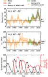Fig. 7. Temporal variations of the amplitude (top panel) and frequency (middle panel) of the HL1 mode, together with the sunspot number and the polar field strength (bottom panel). The orange, green, and red solid curves show the results from MWO, GONG, and HMI data sets, respectively, with the shaded areas showing the 68% confidence interval estimated from 10 000 Monte Carlo simulations. The open circles indicate that the excess power around the mode frequency is below 90% confidence level. The horizontal dashed lines represent the median value over MWO (1968–2010) and HMI (2011–2023) data sets.

5.4. Evolution of mode velocity pattern

In addition to the mode amplitude and frequency, we also measure the slope of the striped pattern seen in the supersynoptic maps of V_zonal at high latitudes. We define the slope of the striped pattern as the ratio of Δτ/Δλ, where Δτ is the time lag between the time series of V_zonal at different latitudes and Δλ is the latitudinal separation thereof, as depicted in the top panel of Fig. 8. In practice we determine the time lag that maximizes the correlation between V_zonal at adjacent latitudes and average over latitude weighted by a raised cosine between latitudes 60° and 75°. The bottom panel of Fig. 8 shows its temporal variation. The measured Δτ/Δλ varies mostly between 0.2 and 1 day/deg with a medium value of 0.56 day/deg. Although there are two points below zero (years 1969 and 1994), they fall within the range of uncertainty. It seems fair to say that Δτ/Δλ does not change sign. The Δτ/Δλ seems to have larger values during solar minima and exhibits an 11-yr variation to some extent, though not as clearly as in the mode amplitude. We note that the time lag Δτ has a dependence on the mode frequency. Nonetheless, the variation in the measured ν_HL1 (about ±5 nHz) only affects Δτ/Δλ by ±1.5% which is negligible.

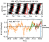Fig. 8. Temporal variations of HL1 mode velocity pattern. Top: HMI $V_{\mathrm{zonal}}^{(-)}$ in the first half of 2021 applied with a band-pass filter around ${\nu }_{HL1}^{\mathrm{synodic}}$. The slope of the striped pattern in $V_{\mathrm{zonal}}^{(-)}$ is highlighted by the tilted red lines. The Δτ (time lag) and Δλ (latitudinal separation) that determine the slope of the striped pattern Δτ/Δλ are indicated in the plot (the two legs of the red right triangle). Bottom: Δτ/Δλ as a function of time, using the same color conventions as in Fig. 7.

5.5. Correlations between mode parameters, sunspot number, and polar field

In order to examine which periodicities that are present in the time series of the HL1 mode parameters, we combine the measurements from MWO (1968–2010) and HMI (2011–2022) to form a 55-yr long data set, and we compute a temporal power spectrum for each of the parameters (velocity amplitude, frequency, and eigenfunction tilt). The right column of Fig. A.4 shows these three power spectra. We see that there is a clear 11-yr periodicity in the mode velocity amplitude, while the power spectrum for the mode frequency does not show a distinct peak at (11 yr)⁻¹ = 2.88 nHz. The second and third plots on the left column of Fig. A.4 highlight (in red) the 11-yr component of the evolution of the velocity amplitude and the tilt. We see that they are anti-correlated with the sunspot number. The correlation coefficients between the mode parameters and the sunspot number are −0.5 for the mode amplitude and −0.34 for the eigenfunction tilt. Since there are only 18 independent points in a period of 55 years, we find that coefficients lower than 0.47 in absolute value are not significant (p > 0.05). Thus only the anticorrelation between the mode amplitude and the sunspot number is significant.

We also compute the correlation coefficients between the mode parameters and the polar field strength over the period 1977–2022 shown in the bottom panel of Fig. 7. Surprisingly, these correlation coefficients are all below 0.1 in absolute value, which means there is no correlation between the mode parameters and the polar field strength.

5.6. Correlations between mode parameters and rotation rate

We now compare the mode parameters with the solar surface rotation rate at 60° latitude where the local rotation rate is close to the mode frequency. From 1996, we use the solar rotation rate obtained from global helioseismology (Larson & Schou 2015, 2018). The data series used are mdi.vw_V_sht_2drls from 1996 to 2010 and hmi.vw_V_sht_2drls from 2010 to 2022, at intervals of 72 days with NACOEFF=6. The rotation rate is smoothed with a 360-day running window. We then extend the measurements back to 1983 using the MWO Doppler velocity data, as processed by Ulrich et al. (2023, their Table 1 and Figure 4). The MWO rotation rate is shifted by an offset of 16 nHz so it matches the near-surface rotation rate from global helioseismology during the overlapping time period. Also, because the global helioseismology data are north-south symmetric by construction, we symmetrize the MWO data. We remark that the surface rotation rate from the MWO Doppler velocity starts from 1983, despite the fact that the MWO Doppler data have been available since 1967. This is because there exists a systematic error that offsets the Doppler signals prior to 1983 (Ulrich et al. 2023, section 2). Since we only consider the signals in the inertial frequency range, this systematic error may not bias the measured mode parameters.

The right panel of Fig. 9 compares the evolution of the mode frequency and the surface rotation rate at 60° latitude for 1983–2023, together with the mode frequency (the shaded region covers the error range of ±1σ). Both curves show the same long-term decrease, which amounts to about −7 nHz over 30 years. This decrease has been reported before at this latitude during cycles 23 and 24 throughout the convection zone (Basu & Antia 2019, their Figure 2). In addition, the rotation rate also shows an 11-year component at the level of ±2.5 nHz associated with the high-latitude branch of the so-called torsional oscillation (e.g., Howe 2009; Howe et al. 2013; Basu 2016). These small variations in the rotation rate are within the error bars of the inertial mode frequency (±3 nHz or so, for a three year time window). The mode frequency measurements are too noisy to reveal any variation at this level of precision. Overall, the correlation coefficient between the mode frequency and the rotation rate at 60° is 0.55. This correlation coefficient is significant (p = 0.05).

The left panel of Fig. 9 compares the evolution of the mode amplitude with the timing of the solar cycles. The times of solar minima are indicated on the plot with vertical bars. We find that the times at which the mode amplitude reaches its maximum coincide with the beginnings of cycles 21, 22, and 25. But when the mode amplitude is smaller (solar minima of cycles 22/23 and 23/24), the mode has its maximum amplitude 1–3 years after the solar minima. Furthermore, cycle 21 is the strongest sunspot cycle in the past five decades and the polar field strength in the subsequent solar minimum is notably strong; however, the mode amplitude is not particularly small in that period. We see that the relative mode amplitude variations are on the order of unity, while the relative change in rotation due to the torsional oscillation is about 1%. We find a correlation coefficient between the mode amplitude and the rotation rate at 60° of −0.82. This anticorrelation is very significant (p = 0.0006).

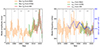Fig. 9. Temporal variation of the mode amplitude (left) and frequency (right) taken from Fig. 7, together with surface rotation rates at 60° latitude obtained from MWO Doppler velocity (1983–2013) in solid light blue, and from global helioseismology using MDI (1996–2010) and HMI (2010–2023) data in dashed blue. The beginnings of cycles 21–25 (solar minima) are marked with vertical lines and the cycle numbers are denoted at the top.

6. Summary and discussion

We have computed synoptic maps of zonal velocity V_zonal using LOS Doppler velocity from MWO, GONG, and HMI, covering a total of 57 years. We have measured the HL1 mode parameters from these synoptic maps at high latitudes. The time series of mode amplitude and eigenfunction tilt exhibit an 11-yr periodicity, whereas the 11-yr periodicity in mode frequency is below noise level. The time series of mode amplitude and eigenfunction tilt are weakly anticorrelated with the sunspot number. However, the anticorrelation with the high-latitude rotation rate is more pronounced, particularly for the mode amplitude. The mode amplitude peaks coincide with solar minima when the mode amplitude is large, but lag by 1–3 years when the mode amplitude is smaller. The long-term trend of the mode frequency follows the rotation rate near the critical latitude. The results presented in this work contain a wealth of information about the HL1 mode. Improved linear and nonlinear models of inertial modes (with magnetic field) are needed to interpret the observations and further constrain the physics of the solar interior.

The temporal changes in mode frequency are very small and can probably be explained using the linearized wave equation together with a prescription of the variations in solar rotation and solar structure. In particular, the solar-cycle variations of rotation (torsional oscillation) are known from p-mode helioseismology throughout the convection zone, and their effect on the HL1 mode frequency can be inferred using a linear eigenvalue solver (Bekki et al. 2022) or a first-order perturbation method (see work by Goddard et al. 2020, for the equatorial Rossby modes). However, it remains to be seen if changes in the rotation alone will be sufficient to explain the data. The changes in the background entropy and the direct effect of the magnetic field on the mode may have some importance as well. In turn, the measurements of mode frequency present an opportunity to constrain these changes in the convection zone (unlike p modes, inertial modes have large kinetic energy density deep in the convection zone).

The much larger variations in mode amplitude and mode eigenfunctions will require more sophisticated modeling tools. Recent non-linear 3D hydrodynamic simulations carried out by Bekki et al. (2024) have revealed the complex relationship between the baroclinically-unstable high-latitude modes, the entropy gradient, and the rotation rate. It was shown that the modes may transport entropy toward the equator and thus back react on the latitudinal differential rotation. Such work represents a first step in the understanding of the dynamics of the HL1 mode, but will have to be extended to account for the effects of the dynamo.

Data availability

Movie associated to Fig. 5 is available at https://www.aanda.org

Acknowledgments

We are very grateful to Roger K. Ulrich for providing the data from the synoptic program at the 150-Foot Solar Tower of the Mt. Wilson Observatory. The Mt. Wilson 150-Foot Solar Tower is operated by UCLA, with funding from NASA, ONR and NSF, under agreement with the Mt. Wilson Institute. The HMI data used are courtesy of NASA/SDO and the HMI science team. SOHO is a project of international cooperation between ESA and NASA. This work utilizes GONG data from the National Solar Observatory (NSO), which is operated by AURA under a cooperative agreement with NSF and with additional financial support from NOAA, NASA, and USAF. The sunspot numbers are from the World Data Center SILSO, Royal Observatory of Belgium, Brussels. The polar magnetic field data are from the Wilcox Solar Observatory (http://wso.stanford.edu/Polar.html), courtesy of J.T. Hoeksema. The Wilcox Solar Observatory is currently supported by NASA. We acknowledge support from ERC Synergy Grant WHOLE SUN 810218. The data were processed at the German Data Center for SDO (GDC-SDO), funded by the German Aerospace Center (DLR). L.G. acknowledges support from the NYU Abu Dhabi Center for Space Science.

References

Appendix A: Additional figures

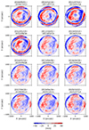Fig. A.1. Median values of the Dopplergrams over the time periods between the HMI retuning dates listed at http://jsoc.stanford.edu/doc/data/hmi/hmi_retuning.txt. The images have been remapped to the same resolution (10″per pixel), with the disk center aligned north-up, and the Vbackground component subtracted. The color scale is saturated at ±50 m/s. Hathaway et al. (2015, their figure 2) shows a similar pattern in the HMI data from 2012 to 2013. The interference fringes appear as wavy patterns in the HMI images, caused by imperfections in the tunable-filter elements of the optical system. These unwanted patterns in the Dopplergrams exceed 50 m/s in magnitude, which is significantly higher than the amplitude of the HL1 mode. The large-scale fringes were substantially removed by the HMI team from 1 October 2012 (Couvidat et al. 2016), which explains why the fringes in the last eight panels are much weaker than in the first four panels. While the temporal frequency of these patterns is very low and far from the HL1 mode frequency, the patterns shift during HMI instrument re-tuning, causing jumps in the Doppler time series and increasing the background power in the Fourier domain. Removing these fringes enhances the visibility of the HL1 mode in the synoptic maps of Vzonal and improves the signal-to-noise ratio of the mode amplitude measurement.

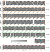Fig. A.2. Synoptic maps of Vzonal as functions of latitude and time, obtained from direct Vlos of HMI, GONG, and MWO observations. For clarity, the maps were Gaussian smoothed in latitude with a FWHM of 10°. The arrows with the same color highlight the stripes for different data sets in the same time period.

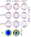Fig. A.3. Comparison of the m = 1 high-latitude mode oscillations in the line-of-sight Doppler velocity as viewed from the Earth, obtained using various methods, when the solar tilt angle B0 is 7.24° (top), 0° (middle), and −7.24° (bottom). Left column: observed Doppler velocity Vlos from HMI data band-pass filtered around ${\nu }_{HL1}^{\mathrm{synodic}}$ ($V_{\mathrm{los}}^{HL1}$, see Eq. (8)). For a better comparison with the middle column, the images were Gaussian smoothed with a FWHM of 5°. Middle column: reconstructed Vlos, obtained by projecting the 5°-tile horizontal flow maps from the HMI ring-diagram analysis onto the line of sight and applying the same filter as in the first column. Right column: line-of-sight projection of mode eigenfunction obtained using a linear eigenvalue solver (Bekki et al. 2022), scaled to an amplitude comparable to the observations. Bottom row: maps of noise in $V_{\mathrm{los}}^{HL1}$ estimated from the temporal variance of the data at each spatial point.

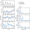Fig. A.4. Eleven-year periodic components and power spectra of HL1 mode parameters. Left column, from top to bottom: sunspot number, HL1 mode amplitude, eigenfunction tilt, and frequency. The 55-yr long time series combine the MWO (1968 – 2010) and HMI (2011 – 2022) measurements taken from Figs. 7 and 8. The gray curves are fitted parabolas representing the long-term trend. The pink curves show the 11-yr periodicity in the data added to the long-term trend. Right column: power spectra of the time series from the left column with the temporal mean subtracted. The vertical pink lines indicate the frequency of (11yr)−1 = 2.88 nHz that corresponds to the average sunspot cycle period. The horizontal dashed and dotted lines represent the 95% and 90% confidence levels, respectively. The 11-year periodicity is highly significant for the mode amplitude, and only marginally significant for the eigenfunction tilt. No evidence is found for an 11-year periodicity in the mode frequency.

All Figures

	Fig. 1. Schematics of data processing steps involved in the measurement of the velocity amplitude of the HL1 mode from MWO, GONG, and HMI time series of Dopplergrams.
In the text

Fig. 2. Example supersynoptic maps of Vzonal in the Earth frame computed from the MWO (top three panels), GONG (fourth panel), and HMI data (bottom panel) near cycle minima. The full data set is shown in Fig. A.2). The HL1 mode may be seen from time to time as stripes in Vzonal above 50° latitude (see regions in red ellipses). For clarity, the maps were smoothed in latitude with a Gaussian kernel of width 10°.

In the text

	Fig. 3. $V_{\mathrm{zonal}}^{(\mathrm{band})}(t)$ during different overlapping periods of the MWO, GONG, and HMI data. The period of the predominant oscillations seen in $V_{\mathrm{zonal}}^{(\mathrm{band})}$ is about 34 days, which corresponds to the HL1 mode frequency near ${\nu }_{HL1}^{\mathrm{synodic}}=338$ nHz.
In the text

	Fig. 4. Power spectra of $V_{\mathrm{zonal}}^{(\mathrm{band})}$ in the frequency range 250–450 nHz (in the Earth frame), computed from the MWO, GONG, and HMI Dopplergrams (from top to bottom respectively). The vertical red lines at 338 nHz mark the reference synodic frequency of the HL1 mode.
In the text

Fig. 5. Line-of-sight Doppler velocity associated with the HL1 mode as viewed from the Earth on 09 September 2018 when the solar tilt angle B0 is 7.24°, extracted from time series of daily HMI images by applying a band-pass filter around ${\nu }_{HL1}^{\mathrm{synodic}}$ (see Eq. (8)). The LOS velocity pattern in the polar regions is associated with the HL1 mode. The image was smoothed using a 2D Gaussian kernel with a FWHM of 5°. A comparison with the reconstructed $V_{\mathrm{los}}^{HL1}$ using 5°-tile ring-diagram flow maps is shown in Fig. A.3 and in the online movie.

In the text

Fig. 6. Visibility of HL1 mode in consecutive three-year power spectra, using MWO (1969–2010) and HMI (2011–2022) data. Panel a: example MWO time series (1984–1986) of $V_{\mathrm{zonal}}^{(-)}$ averaged over latitudes 60° ≤λ < 75° (i.e., $V_{\mathrm{zonal}}^{(\mathrm{band})}$). Panel b: power spectra of $V_{\mathrm{zonal}}^{(-)}$ for the same time period in various latitudinal bands of 15° (labeled at the top right corner of each panel). The vertical red lines denote the reference HL1 mode frequency ${\nu }_{HL1}^{\mathrm{synodic}}=338$ nHz and the excess power around this frequency is highlighted in blue. The shaded pink areas indicate the differential rotation rate in the outer 5% of the Sun from global helioseismology as viewed from the Earth. Panels c and d: same as above but for an example HMI three-year time series during 2017–2019. Panel e: all available three-year power spectra of $V_{\mathrm{zonal}}^{(\mathrm{band})}$ stacked on top of each other. The crosses highlight the reference frequency of 338 nHz.

In the text

Fig. 7. Temporal variations of the amplitude (top panel) and frequency (middle panel) of the HL1 mode, together with the sunspot number and the polar field strength (bottom panel). The orange, green, and red solid curves show the results from MWO, GONG, and HMI data sets, respectively, with the shaded areas showing the 68% confidence interval estimated from 10 000 Monte Carlo simulations. The open circles indicate that the excess power around the mode frequency is below 90% confidence level. The horizontal dashed lines represent the median value over MWO (1968–2010) and HMI (2011–2023) data sets.

In the text

Fig. 8. Temporal variations of HL1 mode velocity pattern. Top: HMI $V_{\mathrm{zonal}}^{(-)}$ in the first half of 2021 applied with a band-pass filter around ${\nu }_{HL1}^{\mathrm{synodic}}$. The slope of the striped pattern in $V_{\mathrm{zonal}}^{(-)}$ is highlighted by the tilted red lines. The Δτ (time lag) and Δλ (latitudinal separation) that determine the slope of the striped pattern Δτ/Δλ are indicated in the plot (the two legs of the red right triangle). Bottom: Δτ/Δλ as a function of time, using the same color conventions as in Fig. 7.

In the text

Fig. 9. Temporal variation of the mode amplitude (left) and frequency (right) taken from Fig. 7, together with surface rotation rates at 60° latitude obtained from MWO Doppler velocity (1983–2013) in solid light blue, and from global helioseismology using MDI (1996–2010) and HMI (2010–2023) data in dashed blue. The beginnings of cycles 21–25 (solar minima) are marked with vertical lines and the cycle numbers are denoted at the top.

In the text

Fig. A.1. Median values of the Dopplergrams over the time periods between the HMI retuning dates listed at http://jsoc.stanford.edu/doc/data/hmi/hmi_retuning.txt. The images have been remapped to the same resolution (10″per pixel), with the disk center aligned north-up, and the Vbackground component subtracted. The color scale is saturated at ±50 m/s. Hathaway et al. (2015, their figure 2) shows a similar pattern in the HMI data from 2012 to 2013. The interference fringes appear as wavy patterns in the HMI images, caused by imperfections in the tunable-filter elements of the optical system. These unwanted patterns in the Dopplergrams exceed 50 m/s in magnitude, which is significantly higher than the amplitude of the HL1 mode. The large-scale fringes were substantially removed by the HMI team from 1 October 2012 (Couvidat et al. 2016), which explains why the fringes in the last eight panels are much weaker than in the first four panels. While the temporal frequency of these patterns is very low and far from the HL1 mode frequency, the patterns shift during HMI instrument re-tuning, causing jumps in the Doppler time series and increasing the background power in the Fourier domain. Removing these fringes enhances the visibility of the HL1 mode in the synoptic maps of Vzonal and improves the signal-to-noise ratio of the mode amplitude measurement.

In the text

	Fig. A.2. Synoptic maps of Vzonal as functions of latitude and time, obtained from direct Vlos of HMI, GONG, and MWO observations. For clarity, the maps were Gaussian smoothed in latitude with a FWHM of 10°. The arrows with the same color highlight the stripes for different data sets in the same time period.
In the text

Fig. A.3. Comparison of the m = 1 high-latitude mode oscillations in the line-of-sight Doppler velocity as viewed from the Earth, obtained using various methods, when the solar tilt angle B0 is 7.24° (top), 0° (middle), and −7.24° (bottom). Left column: observed Doppler velocity Vlos from HMI data band-pass filtered around ${\nu }_{HL1}^{\mathrm{synodic}}$ ($V_{\mathrm{los}}^{HL1}$, see Eq. (8)). For a better comparison with the middle column, the images were Gaussian smoothed with a FWHM of 5°. Middle column: reconstructed Vlos, obtained by projecting the 5°-tile horizontal flow maps from the HMI ring-diagram analysis onto the line of sight and applying the same filter as in the first column. Right column: line-of-sight projection of mode eigenfunction obtained using a linear eigenvalue solver (Bekki et al. 2022), scaled to an amplitude comparable to the observations. Bottom row: maps of noise in $V_{\mathrm{los}}^{HL1}$ estimated from the temporal variance of the data at each spatial point.

In the text

Fig. A.4. Eleven-year periodic components and power spectra of HL1 mode parameters. Left column, from top to bottom: sunspot number, HL1 mode amplitude, eigenfunction tilt, and frequency. The 55-yr long time series combine the MWO (1968 – 2010) and HMI (2011 – 2022) measurements taken from Figs. 7 and 8. The gray curves are fitted parabolas representing the long-term trend. The pink curves show the 11-yr periodicity in the data added to the long-term trend. Right column: power spectra of the time series from the left column with the temporal mean subtracted. The vertical pink lines indicate the frequency of (11yr)−1 = 2.88 nHz that corresponds to the average sunspot cycle period. The horizontal dashed and dotted lines represent the 95% and 90% confidence levels, respectively. The 11-year periodicity is highly significant for the mode amplitude, and only marginally significant for the eigenfunction tilt. No evidence is found for an 11-year periodicity in the mode frequency.

In the text

References

- Basu, S. 2016, Liv. Rev. Sol. Phys., 13, 2 [Google Scholar]
- Basu, S., & Antia, H. M. 2019, ApJ, 883, 93 [Google Scholar]
- Bekki, Y., Cameron, R. H., & Gizon, L. 2022, A&A, 662, A16 [NASA ADS] [CrossRef] [EDP Sciences] [Google Scholar]
- Bekki, Y., Cameron, R. H., & Gizon, L. 2024, Sci. Adv., 10, eadk5643 [NASA ADS] [CrossRef] [Google Scholar]
- Bogart, R. S., Baldner, C., Basu, S., Haber, D. A., & Rabello-Soares, M. C. 2011a, in GONG-SoHO 24: A New Era of Seismology of the Sun and Solar-Like Stars (IOP), J. Phys. Conf. Ser., 271, 012008 [NASA ADS] [Google Scholar]
- Bogart, R. S., Baldner, C., Basu, S., Haber, D. A., & Rabello-Soares, M. C. 2011b, in GONG-SoHO 24: A New Era of Seismology of the Sun and Solar-Like Stars (IOP), J. Phys. Conf. Ser., 271, 012009 [NASA ADS] [Google Scholar]
- Bogart, R. S., Baldner, C. S., & Basu, S. 2015, ApJ, 807, 125 [NASA ADS] [CrossRef] [Google Scholar]
- Couvidat, S., Schou, J., Hoeksema, J. T., et al. 2016, Sol. Phys., 291, 1887 [Google Scholar]
- Fournier, D., Gizon, L., & Hyest, L. 2022, A&A, 664, A6 [NASA ADS] [CrossRef] [EDP Sciences] [Google Scholar]
- Gizon, L. 2004, Sol. Phys., 224, 217 [Google Scholar]
- Gizon, L., Cameron, R. H., Bekki, Y., et al. 2021, A&A, 652, L6 [NASA ADS] [CrossRef] [EDP Sciences] [Google Scholar]
- Gizon, L., Bekki, Y., Birch, A. C., et al. 2024, in Dynamics of Solar and Stellar Convection Zones and Atmospheres, eds. A. V. Getling, & L. L. Kitchatinov, IAU Symp., 365, 207 [NASA ADS] [Google Scholar]
- Goddard, C. R., Birch, A. C., Fournier, D., & Gizon, L. 2020, A&A, 640, L10 [NASA ADS] [CrossRef] [EDP Sciences] [Google Scholar]
- Hanson, C. S., Hanasoge, S., & Sreenivasan, K. R. 2022, Nat. Astron., 6, 708 [NASA ADS] [CrossRef] [Google Scholar]
- Harvey, J. W., Hill, F., Hubbard, R. P., et al. 1996, Science, 272, 1284 [Google Scholar]
- Hathaway, D. H., Upton, L., & Colegrove, O. 2013, Science, 342, 1217 [NASA ADS] [CrossRef] [Google Scholar]
- Hathaway, D. H., Teil, T., Norton, A. A., & Kitiashvili, I. 2015, ApJ, 811, 105 [Google Scholar]
- Hoeksema, J. T., Baldner, C. S., Bush, R. I., Schou, J., & Scherrer, P. H. 2018, Sol. Phys., 293, 45 [NASA ADS] [CrossRef] [Google Scholar]
- Howe, R. 2009, Liv. Rev. Sol. Phys., 6, 1 [Google Scholar]
- Howe, R., Christensen-Dalsgaard, J., Hill, F., et al. 2013, ApJ, 767, L20 [NASA ADS] [CrossRef] [Google Scholar]
- Larson, T. P., & Schou, J. 2015, Sol. Phys., 290, 3221 [NASA ADS] [CrossRef] [Google Scholar]
- Larson, T. P., & Schou, J. 2018, Sol. Phys., 293, 29 [Google Scholar]
- Lekshmi, B., Gizon, L., Jain, K., Liang, Z. C., & Philidet, J. 2024, in Dynamics of Solar and Stellar Convection Zones and Atmospheres, eds. A. V. Getling, & L. L. Kitchatinov, IAU Symp., 365, 230 [NASA ADS] [Google Scholar]
- Löptien, B., Gizon, L., Birch, A. C., et al. 2018, Nat. Astron., 2, 568 [Google Scholar]
- Scherrer, P. H., Schou, J., Bush, R. I., et al. 2012, Sol. Phys., 275, 207 [Google Scholar]
- Ulrich, R. K. 1993, in IAU Colloq. 137: Inside the Stars, eds. W. W. Weiss, & A. Baglin, ASP Conf. Ser., 40, 25 [NASA ADS] [Google Scholar]
- Ulrich, R. K. 2001, ApJ, 560, 466 [CrossRef] [Google Scholar]
- Ulrich, R. K., Boyden, J. E., Webster, L., et al. 1988, Sol. Phys., 117, 291 [NASA ADS] [CrossRef] [Google Scholar]
- Ulrich, R. K., Tran, T., & Boyden, J. E. 2023, Sol. Phys., 298, 123 [NASA ADS] [CrossRef] [Google Scholar]
- Waidele, M., & Zhao, J. 2023, ApJ, 954, L26 [NASA ADS] [CrossRef] [Google Scholar]