| Issue |
A&A
Volume 665, September 2022
|
|
|---|---|---|
| Article Number | A34 | |
| Number of page(s) | 22 | |
| Section | Extragalactic astronomy | |
| DOI | https://doi.org/10.1051/0004-6361/202243249 | |
| Published online | 06 September 2022 | |
COSMOS2020: Manifold learning to estimate physical parameters in large galaxy surveys
1
Cosmic Dawn Center (DAWN), Denmark
2
Niels Bohr Institute, University of Copenhagen, Jagtvej 128, 2200 Copenhagen N, Denmark
e-mail: This email address is being protected from spambots. You need JavaScript enabled to view it.
3
Núcleo de Astronomía de la Facultad de Ingeniería y Ciencias, Universidad Diego Portales, Av. Ejército Libertador 441, Santiago, Chile
e-mail: This email address is being protected from spambots. You need JavaScript enabled to view it.
4
Aix Marseille Univ., CNRS, CNES, LAM, Marseille, France
5
California Institute of Technology, Pasadena, CA 91125, USA
6
Jet Propulsion Laboratory, California Institute of Technology, Pasadena, CA 91109, USA
7
Leiden Observatory, Leiden University, PO Box 9513 2300 RA Leiden, The Netherlands
8
Sorbonne Université, CNRS, UMR 7095, Institut d’Astrophysique de Paris, 98 bis Bd Arago, 75014 Paris, France
9
Infrared Processing and Analysis Center, California Institute of Technology, Pasadena, CA 91125, USA
10
DTU-Space, Technical University of Denmark, Elektrovej 327, 2800 Kgs. Lyngby, Denmark
11
National Centre for Nuclear Research, ul. Pasteura 7, 02-093 Warszawa, Poland
12
Physics and Astronomy Department, University of California, 900 University Avenue, Riverside, CA 92521, USA
13
Institute for Astronomy, University of Hawaii, 2680 Woodlawn Drive, Honolulu, HI 96822, USA
Received:
2
February
2022
Accepted:
6
June
2022
Abstract
We present a novel method for estimating galaxy physical properties from spectral energy distributions (SEDs) as an alternative to template fitting techniques and based on self-organizing maps (SOMs) to learn the high-dimensional manifold of a photometric galaxy catalog. The method has previously been tested with hydrodynamical simulations in Davidzon et al. (2019, MNRAS, 489, 4817), however, here it is applied to real data for the first time. It is crucial for its implementation to build the SOM with a high-quality panchromatic data set, thus we selected “COSMOS2020” galaxy catalog for this purpose. After the training and calibration steps with COSMOS2020, other galaxies can be processed through SOMs to obtain an estimate of their stellar mass and star formation rate (SFR). Both quantities resulted in a good agreement with independent measurements derived from more extended photometric baseline and, in addition, their combination (i.e., the SFR vs. stellar mass diagram) shows a main sequence of star-forming galaxies that is consistent with the findings of previous studies. We discuss the advantages of this method compared to traditional SED fitting, highlighting the impact of replacing the usual synthetic templates with a collection of empirical SEDs built by the SOM in a “data-driven” way. Such an approach also allows, even for extremely large data sets, for an efficient visual inspection to identify photometric errors or peculiar galaxy types. While also considering the computational speed of this new estimator, we argue that it will play a valuable role in the analysis of oncoming large-area surveys such as Euclid of the Legacy Survey of Space and Time at the Vera C. Rubin Telescope.
Key words: galaxies: fundamental parameters / galaxies: star formation / galaxies: stellar content / methods: observational / astronomical databases: miscellaneous
© I. Davidzon et al. 2022
 Open Access article, published by EDP Sciences, under the terms of the Creative Commons Attribution License (https://creativecommons.org/licenses/by/4.0), which permits unrestricted use, distribution, and reproduction in any medium, provided the original work is properly cited.
This article is published in open access under the Subscribe-to-Open model. This email address is being protected from spambots. You need JavaScript enabled to view it. to support open access publication.
1. Introduction
Redshift (z), stellar mass (M), and star formation rate (SFR) are fundamental parameters in studies of galaxy evolution. Measuring these quantities has been instrumental to the discovery of the main sequence of star-forming galaxies (Brinchmann et al. 2004; Noeske et al. 2007; Elbaz et al. 2007; Daddi et al. 2007), namely, a tight correlation between M and SFR pointing to a “steady” mechanism of gas-to-stars conversion at work in systems that have gone through different evolutionary paths. Other examples include the SFR and stellar mass functions, two demographics that can be computed for galaxies in different redshift bins and are commonly used to either calibrate or validate cosmological simulations (e.g., Henriques et al. 2013; Furlong et al. 2015; Katsianis et al. 2017; Davé et al. 2017).
In the absence of spectroscopic data, which demand more telescope time than broadband photometry, these three quantities can be derived by fitting galaxy templates to the observed spectral energy distribution (SED). Those templates are built via stellar population synthesis models (e.g., Bruzual & Charlot 2003; Maraston 2005; Conroy et al. 2009), assuming a grid of ages and metallicity values, different star formation histories (SFHs), and one or more options for dust attenuation (for a review, see Conroy 2013). With respect to redshift and stellar mass, SED fitting is a standard practice that produces robust results even when the input photometry is limited to a few bands in the optical and near-infrared (NIR) regime (for a review, see Salvato et al. 2019). The method is sub-optimal for constraining SFR, unless far-infrared (FIR) data are included (Pannella et al. 2009; Buat et al. 2010; Riccio et al. 2021). However, sky coverage and depth of FIR ancillary data should match those of surveys at shorter wavelengths, a condition that is satisfied in only a few extragalactic fields.
Another way to estimate the SFR is to rely on machine learning techniques (ML). For example, a galaxy catalog can be processed through a neural network previously trained with a sample of objects whose physical properties are already known (Davidzon et al. 2019; Surana et al. 2020; Gilda et al. 2021; Simet et al. 2021). This means that the targets can be compared to other observed galaxies, instead of synthetic templates, with the advantage of adhering more coherently to the observational parameter space. In many cases, the training sample is also more accurate than standard templates because its features come directly from high-quality data (e.g., a spectroscopic sample such as the Sloan Digital Sky Survey, Acquaviva 2016) instead of approximated models. On the other hand, such a data-driven approach provides limited physical insights and may introduce an observational bias if the ML algorithm is not trained on a fully representative sample. A possible solution to this drawback is to use a training sample built from cosmological simulations (e.g., mock photometry or spectra, Lovell et al. 2019; Simet et al. 2021) even though providing galaxy models with “observational-like” properties, as well as realistic error bars, is a complex task (see discussion in Laigle et al. 2019).
The present study shows the advantages of a ML-based method built on previous work published in Masters et al. (2015), Hemmati et al. (2019a), and Davidzon et al. (2019) to predict galaxy properties. The method involves dimensionality reduction through self-organizing maps (SOMs, Kohonen 1981) and has been previously tested in Davidzon et al. (2019) based on a mock galaxy catalog (derived from hydrodynamical simulations, see Laigle et al. 2019). Knowing the intrinsic properties of those simulated galaxies, (Davidzon et al. 2019) proved that the SOM can serve as an effective “manifold learning” tool that is able to explore the complex, non-linear galaxy parameter space and reproduce an approximated, but still accurate, version in a low-dimensional space. We are now ready to apply the same method to real data and judge its performance in a practical “user case” situation.
In a nutshell, we used the SOM to analyze a multi-dimensional space made by the combination of galaxy colors in the observer’s frame between 0.3 and 5 μm. This data set is a combination of two photometric catalogs in distinct survey fields, already described in previous work (Mehta et al. 2018; Weaver et al. 2022) and summarized here in Sect. 2. The SOM returns an “unsupervised” classification of the input galaxy sample, namely, the various classes (which will be called “cells”) are formed without making any comparisons to already classified examples. The second step does require supervision, since at least a fraction of the galaxies require a label (from ancillary data, especially Spitzer/MIPS) to determine the physical properties of each SOM cell. This set-up allows us to assign the following labels: z, M, SFR, to any new object projected onto the SOM. More details about the method are provided in Sect. 3.
In Sect. 4, we verify that SOM-based estimates are more precise than what would result from fitting a standard template library to the same optical-NIR photometry. This section also presents the resulting main sequence of star-forming galaxies up to z = 2, and a comparison with previous studies where SFRs have been derived in different ways. Further extensions and other potential applications of our SOM-based method are discussed in Sect. 5, along with a few caveats. We summarize our work and draw our conclusions in Sect. 6.
Throughout this work we use a flat ΛCDM cosmology with H0 = 70 km s−1 Mpc−1, Ωm = 0.3, ΩΛ = 0.7. All magnitudes are in the AB (Oke 1974) system, and the initial mass function (IMF) assumed here is the one proposed in Chabrier (2003). In the quoted scaling relations between SFR and rest-frame luminosities, the latter are in units of L⊙ ≡ 3.826 × 1033 erg s−1 for the former to be in M⊙ yr−1.
2. Data
The present study relies on two catalogs built from deep photometric surveys in the Subaru XMM/Newton and Cosmic Evolution Survey fields (Furusawa et al. 2008; Scoville et al. 2007, SXDF and COSMOS, see respectively). The two extragalactic fields, each of them on the order of a square degree, are particularly suited to our ML application: they can be easily used in tandem because they have in common a subset of galaxy colors spanning from UV to mid-infrared (MIR). In the present analysis, we are especially interested in broadband photometry since the galaxy colors derived from it are the features used as input by the SOM. In the last two decades COSMOS has been targeted by numerous telescopes, producing a wealth of ancillary data beyond MIR. The observations in the COSMOS field are also extremely deep, and likely to increase depth even further in the near future owing to planned surveys with both existing and oncoming facilities. For these reasons, a catalog of COSMOS galaxies is ideal for training and calibrating the SOM (Sects. 3.1 and 3.2). On the other hand, SXDF galaxies serve as a test sample to verify the reliability of our method (Sect. 3.3). The advantages of such a strategy, relying on multiple layers of independent data with increasing depth, have been illustrated for instance, in Myles et al. (2021).
2.1. SXDF2018 photometric catalog
Published in Mehta et al. (2018), the “SXDF2018” photometric catalog includes optical images from the first data release (DR1) of the Hyper-SuprimeCam Subaru Strategic Program (HSC-SSP, Aihara et al. 2018) and MUSUBI, the MegaCam Ultra-deep Survey with U-Band Imaging1 carried out at the Canada-France-Hawaii Telescope (CFHT). In the NIR regime, images come from the ultra-deep area of the UKIRT Infrared Deep Sky Survey (UKIDSS-UDS, Lawrence et al. 2007) and from the VISTA Deep Extragalactic Observations (VIDEO, Jarvis et al. 2013). The entire area is also covered by the Spitzer Space Telescope, with several IRAC programs documented in Euclid Collaboration (2022). The broadbands used here, along with their 5σ sensitivity limits, are listed in Table 1. We refer to Mehta et al. (2018) for further details.
Optical and NIR data building the observer-frame color space explored by the SOM.
2.2. COSMOS2020 photometric catalog
COSMOS2020 is the latest photometric catalog released by the COSMOS collaboration (Weaver et al. 2022). Two versions of the catalog have been produced through different source extraction methods. Here we use the CLASSIC version based on SourceExtractor (Bertin & Arnouts 1996) and IRACLEAN (Hsieh et al. 2012), since that pipeline is similar to the one applied to SXDF20182 The COSMOS field is covered by the same instruments and bands mentioned in Sect. 2.1, although here they are generally deeper than in SXDF (see Table 1). In particular, HSC-SSP images come from an updated release (DR2, Aihara et al. 2019) while the NIR is covered by UltraVISTA (McCracken et al. 2012) with an exposure time per pixel > 150 h (compared to the 10−20 h of VIDEO). The UltraVISTA depth is not homogeneous, that is, there are “Deep” and “Ultra-Deep” areas but Shuntov et al. (2022) showed that at low redshift they can be safely combined in a joint analysis, if this is limited to magnitudes brighter than the Deep 3σ limit (see Table 1). Medium- and narrow-band images from Subaru and VISTA telescopes are also available in COSMOS, as well as GALEX data from Zamojski et al. (2007). These additional bands are taken into account for template fitting (see below) whereas they are not part of the SOM analysis. VISTA observations in COSMOS have been carried out with a dual-layer strategy; therefore, the table provides two values for Y, J, H, and Ks depths. More details about COSMOS2020 can be found in Weaver et al. (2022).
2.3. Physical properties of COSMOS2020 galaxies
As the reference sample for SOM training and calibration, COSMOS2020 galaxies must be provided not only with broadband colors but also with measurements of key physical properties. Most of this additional information is extracted by fitting the observed SED with galaxy models (also known as templates). Namely, the fitting code LePhare (Arnouts et al. 1999; Ilbert et al. 2006) is used with three different configurations to derive: (1) photometric redshifts (zLePh); (2) stellar masses (MLePh) and absolute magnitudes; (3) star formation rates only for sources observed in FIR. Each step is summarized below. Estimates (1) and (2) are described more extensively in Weaver et al. (2022) while we implement the third step following Ilbert et al. (2015). Since information on the FIR regime – namely, a 24 μm detection with Spitzer/MIPS – is required to constrain star formation, (3) can be applied only to a subsample of galaxies (see Fig. 1).
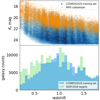 |
Fig. 1. Observational properties of the galaxy samples used throughout this work. Upper panel: magnitude-redshift distribution of the COSMOS2020 galaxy sample used to train the SOM (blue color map with hexagonal pixels) after pre-selection at Ks < 24.8 and log(M/M⊙)> 8.5. Individual sources with a 5σ detection in MIPS are overplotted as orange dots. Lower panel: photometric redshift distribution of the COSMOS2020 training set (blue histogram) and the SXDF2018 target sample (green). These data sets are described in Sects. 2.1 and 2.2. |
Redshift. In this first run of LePhare, the observed SED is interpolated by a library of 33 galaxy templates (originally proposed in Ilbert et al. 2013). The intrinsic spectrum of these templates is modified by a dust screen ranging from E(B − V)=0 to 0.5, with different options to model the extinction curve (Prevot et al. 1984; Calzetti et al. 2000, and two variations of Calzetti’s law including the 2175 Å bump). A complementary library of stellar templates is used, together with other criteria3, to remove stars from the catalog. After evaluating the χ2 of each fit, the resulting zLePh estimates are defined as the median of the redshift likelihood function, i.e. the combined probabilities from the various models (each one ∝e−χ2).
Stellar mass and other physical properties. After fixing the redshift of each source to zLePh, the LePhare code is used to measure galaxy stellar mass. Templates optimized for such a task are derived from Bruzual & Charlot (2003) models (BC03 hereafter) as done in Laigle et al. (2016), namely, with a grid of 44 time steps for eight star formation histories, two non-evolving metallicity values (Z⊙ and 0.2 Z⊙), and a range of dust extinction parameters similar to the one adopted in the first configuration. Absolute magnitudes in different broad-band filters, required to compute rest-frame colors, are an additional output. They are derived from the apparent magnitude that most closely samples the desired rest-frame filter. For example, the observed i band is used to calculate the rest-frame u magnitude for a galaxy at zLePh ≃ 1. When needed, a k-correction is calculated from the best-fit template, which also provides the apparent magnitude of the object when SourceExtractor cannot measure it in any band.
The same run of LePhare would also provide SFRLePh, but we deem the FIR-based estimates more robust for the calibration of our method as will be discussed in Sect. 3.2. Nonetheless, the SFRLePh values are stored in output to compare to the SOM-based estimates derived from the same photometric baseline.
Star formation from infrared continuum. A major role in our analysis is played by the star formation tracer that leverages the correlation between SFR and rest-frame emission in UV and infrared (hereafter SFRUVIR). Interstellar dust absorbs stellar light from UV to optical and re-emits those photons mostly between 8 and 1000 μm, namely, in the infrared (IR) and sub-mm regime. The IR integrated luminosity (LIR) is therefore closely (albeit indirectly) linked with star formation activity. We derived the LIR for COSMOS2020 galaxies as in Ilbert et al. (2015) using FIR data as an observational constraint. In brief, we assign a 24 μm flux to 28 347 objects over the whole COSMOS area via a cross-correlation between COSMOS2020 sources and the Spitzer/MIPS catalog from Le Floc’h et al. (2009). We cut the parent sample at zLePh < 1.8 and signal-to-noise ratio S/N > 5 in the 24 μm band. The redshift upper limit ensures that the polycyclic aromatic hydrocarbons (PAH) complex at a rest-frame of 6.2−7.7 μm does not contaminate the 24 μm measurements. We also removed sources with an X-ray counterpart to minimize contamination from their active galactic nucleus (AGN). The remaining 22 571 MIPS galaxies constitute the calibration sample to enable the SFR estimation with the SOM.
The LIR estimates are obtained by means of LePhare by fitting Dale & Helou (2002) templates to the MIPS data4, then integrating the best-fit model in the rest frame between 8 and 1000 μm. For 7% of them there is also a 5σ detection in Herschel/PACS (either 100 or 160 μm from Lutz et al. 2011), while 9% have a counterpart in Herschel/SPIRE (250, 350, or 500 μm from Oliver et al. 2012). During this procedure, the redshift is fixed to the zLePh value from the optical-NIR fitting. No systematic effect is introduced when the 24 μm flux is complemented with Herschel measurements up to 500 μm (Fig. 1 of Ilbert et al. 2015). Unobscured star formation is traced by the luminosity in the near-UV band (LNUV), which is obtained from the BC03 template fitting described above. Accounting for both contributions, we eventually compute the total SFR as in Arnouts et al. (2013):
 (1)
(1)
where 𝒦 = 8.6 × 10⁻¹¹. This equation traces star formation on a ∼100 Myr time scale. The capability of MIPS 24 μm to provide reliable SFR estimates is also discussed in detail in Rieke et al. (2009).
Alternate SFRUVIR estimates for both COSMOS and SXDF galaxies are available from Barro et al. (2019), although only in the sub-region that was also observed by the Cosmic Assembly Near-infrared Deep Extragalactic Legacy Survey (CANDELS, Grogin et al. 2011; Koekemoer et al. 2011). In addition to ground-based facilities, CANDELS includes data from the Hubble Space Telescope (HST) in both optical and near-IR bands, which may generate some difference in template fitting results (especially photometric redshifts). The ancillary Spitzer and Herschel data in Barro et al. (2019) are similar to the one used here. At z < 1.8 there are 509 (608) matches between Barro et al. (2019) and our COSMOS (SXDF) catalog if we require their photometric redshifts to be within ±30% of zLePh. In COSMOS, after converting the two sets of SFRUVIR estimates to a common framework5 we find a scatter of 0.17 dex and a small systematic offset (−0.03 dex) due to a handful of objects overestimated by Barro et al. (2019) (Fig. B.2). Although the SOM will be calibrated only with LePhare outcomes to ensure consistency, these alternate estimates will play an important role for testing (Sect. 4.2).
2.4. Selection functions
The COSMOS2020 training sample is limited to galaxies outside masked areas of the survey (i.e., avoiding the surroundings of bright stars6) and with zLePh < 1.8 to be consistent with the MIPS-detected sample. In principle, it would be possible to extend the SOM to higher redshift, but in that case the calibration would require a different SFR proxy (see Sect. 5.3). We also cut the training sample at Ks < 24.8 to remove objects with a low signal-to-noise ratio (S/N). Eventually, the COSMOS training sample includes 174 522 galaxies, with 13% of them being MIPS-detected.
We apply a 3σ cut also to the SXDF2018 catalog, corresponding to a Ks < 24.2 limit (see Table 1). Since the goal is to replace LePhare physical properties with SOM estimates, and not the photometric redshifts obtained beforehand, we have the latter ones at our disposal to limit the SXDF2018 sample to zLePh < 1.8 and exclude stellar-like objects. As a result, there are 208 404 galaxies in the SXDF field used, as detailed in the following.
3. Methods
3.1. Training the SOM with COSMOS2020
The SOM can identify data patterns in a multi-dimensional feature space by sampling it with an adaptive distribution of points called “weights”7. During a training phase, the coordinates of these weights in the multi-dimensional space are adjusted to move them close to the input data, according to a convergence criterion detailed in Davidzon et al. (2019). After that, the SOM reproduces not only the “shape” of the input manifold but also its “density”, that is, a larger number of test particles is located where data are more clustered. The algorithm is self-organizing because the training is unsupervised. The SOM maps the input data set into a lower-dimensional space: first, its network is arranged in a 2D geometry then data will be re-arranged as well, each entry being associated with a given test particle. Despite the discretization due to the finite number of test particles, the dimensionality reduction preserves most of the topological structure of the original manifold. The 2D geometry we chose8 is a square grid (see Fig. 2); therefore throughout this study we refer to the SOM test particles as “cells”. With the manifold’s topology mostly preserved, elements that are close to each other in the higher-dimensional space are also neighbors in the grid, namely, they belong to the same cell or two contiguous cells (see a pedagogical illustration in Fig. 3). We refer to the seminal work of Kohonen (1981) for a more extensive explanation.
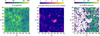 |
Fig. 2. SOM of COSMOS2020 galaxies at z < 1.8, selected as described in Sect. 3.1. The same grid is color-coded in three different ways, to show the number of galaxies per cell (left panel), the similarity between galaxies in a given cell and the correspondent SOM weight (middle panel), and the MIPS-detected objects with MLePh > 1010 M⊙ (right panel). In each grid, empty cells are white. Left: handful of cells with only one or two objects are colored in gray. Middle: similarity is quantified by means of Eq. (2). Throughout this work, the dimensions of the 2D grid are arbitrarily labeled D1 and D2 since they have no physical meaning. |
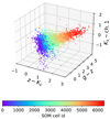 |
Fig. 3. Illustration of the relationship between input features and the SOM classification (made by the so-called “cells”). This simplified example shows only three broadband colors in the observer’s frame, for a random subsample of 10 000 COSMOS2020 galaxies. |
The feature space consists of eleven colors in the observer’s frame, derived from the broadband filters listed in Table 1 and paired in sequential order: u − g, g − r, ..., Ks − ch1, ch1 − ch2. Galaxies are associated with their nearest weight according to their (11-dimensional) Euclidean distance. The ones linked to the same weight are expected to have similar SEDs by construction (see Fig. 1 in Masters et al. 2015) modulo their brightness (i.e., a normalization factor) and the scatter due to photometric errors. The COSMOS2020 SOM is presented in Fig. 2.
The weight’s coordinates in the multi-dimensional space are actually a set of eleven colors, which can be regarded as the “prototype” SED of the cell. This terminology is the same used in Davidzon et al. (2019, see their Table 1). Similarly to that study, shape and size of the grid are chosen in order to minimize the dispersion of data within a given cell, but at the same time to avoid a large fraction of them being empty. The result is a configuration with 80 × 80 cells, with nearly 94% of them containing at least ten objects at the end of the training (Fig. 2, left panel). Number counts vary across the grid by maximum an order of magnitude and only 14 cells have less than three galaxies (one of them being empty).
To quantify the accuracy of the 80 × 80 SOM grid in describing the COSMOS2020 manifold, we calculate the Euclidean distance between galaxies and the weight of the cell associated with them. Namely:
 (2)
(2)
where fi is a galaxy’s feature in the ith dimension (out of Ndim = 11) and wi is one component of the weight representing the cell where the galaxy lies. Across the grid the average Δ per cell is < 1 (Fig. 2, middle panel) as it should be if the scatter of observed SEDs around their weight is dominated by photometric uncertainties, which for the chosen broadband colors are typically 0.05−0.1 mag. A few cells, however, present larger Δ values, an indication they contain either a wider variety of galaxy types or SEDs with similar shapes but a low S/N ratio. As an example, a couple of those cells will be inspected in Sect. 5.4. We also verify that galaxies that are close to each other in the feature space turn out to be in the same (or nearby) cells, as partially shown in Fig. 3. Another metric with which to quantify goodness of fit is the reduced χ2 distance used, for instance, in Masters et al. (2015). This is further discussed in Appendix B (see in particular Fig. B.1).
To conclude the presentation of the training sample, the third (right-hand) panel of Fig. 2 shows the MIPS-detected galaxies in COSMOS. This subsample is spread over 3561 cells (55.6% of the total) which are mainly located on the right half of the grid (see Fig. 2, right panel). One third of the cells probed by MIPS galaxies contain only one of them. Most of these undersampled cells define the boundaries of star-forming regions in the SOM, while others are scattered across the left side of the grid, an area that is scarcely occupied because of the MIPS selection function. In fact, those are cells containing galaxies with i > 23 mag and MLePh < 1010 M⊙ (see discussion in Appendix B and Fig. B.3). Most of them are expected to be fainter than the survey sensitivity limit at 24 μm, as can be deduced, for instance, from Le Floc’h et al. (2009) and Kokorev et al. (2021).
3.2. SOM calibration with physical properties
The cells in a trained SOM can be calibrated a posteriori with redshift values (see e.g., Geach 2012; Masters et al. 2015) or other physical parameters (Hemmati et al. 2019a; Davidzon et al. 2019). We choose the labels to be redshift, stellar mass, SFR, and quiescent versus star-forming galaxy type; these four “layers” of classification are shown with different color codes in Fig. 4.
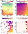 |
Fig. 4. Different sets of labels added to the SOM, after training it with COSMOS2020 data. Upper left: redshift labels assigned from the median zLePh of galaxies in the given cell. Upper right: median log(Mlabel/M⊙) per cell, where the Mlabel values are galaxy stellar masses obtained after rescaling every SED to i = 22.5 (Eq. (3)). Lower left: labels from the median SFRlabel per cell applying the same 22.5 mag rescaling as for stellar mass (Eq. (4)); with respect to Fig. 2, a larger portion of the SOM grid is empty because we did not assign a SFRlabel to cells containing only one MIPS galaxy. Lower right: fraction of quiescent galaxies per cell, according to the NUVrK classification (Eq. (5)). |
For a given cell, the label for each of these quantities is calculated using galaxies inside it. For redshift and stellar mass, this is defined as the median of the zLePh and the normalized MLePh distribution, respectively (Fig. 4, upper panels). The reason for normalizing the mass is discussed in Davidzon et al. (2019). Their simulations show that when the SOM is trained with colors, objects in the same cell have similar mass-to-light ratios while still spanning a range of stellar masses (see Appendix B). We proceed as in Davidzon et al. (2019), namely, by rescaling MLePh estimates to 22.5 mag in the i band:
 (3)
(3)
where mi is the original i-band magnitude of the given galaxy. The median of the Mi = 22.5 distribution in a given cell is used as its label (Mlabel). In the upper-right panel of Fig. 4 the SOM is color-coded according to that label set, showing a smooth transition from 108 M⊙ in the upper-left corner of the grid, corresponding to z ∼ 0, up to 1012 M⊙ in the bottom right. This trend follows, as expected, the evolution in the z label: the higher the redshift, the larger the stellar mass at the fixed 22.5 mag reference.
Regarding galaxy star formation, the calibration is done by using only objects with an available SFRUVIR estimate. A rescaling similar to Eq. (3) is applied for the same reason: galaxies in any given cell have similar colors by SOM construction, but this does not prevent them from freely spanning a certain magnitude range. Therefore, we define:
 (4)
(4)
and we attach a SFRlabel value to the cell based on the median of the SFRi = 22.5 distribution. We disregard cells containing only one MIPS-detected galaxy. The resulting labels are shown in Fig. 4 (lower-left panel).
Each COSMOS2020 galaxy can also be classified as quiescent or active depending on its location in the rest-frame plane NUV − r versus r − Ks (NUVrK, Arnouts et al. 2013). This diagnostic is one of the most common in the literature, together with U − V versus V − J (UVJ, Williams et al. 2009). Either diagram can single out quiescent galaxies from other types as the former ones occupy a delimited locus in the color-color spaces. The advantages of NUV − r with respect to U − V are discussed, for instance, in Siudek et al. (2018) and Leja et al. (2019a). We use the rest-frame NUVrK classification as in Ilbert et al. (2015), where quiescent galaxies have:
 (5)
(5)
with C ≡ 0.17(t − tz = 2) being a cosmic time-dependent correction to maintain consistent criteria across the whole redshift range. From Eq. (5), we derive the fraction of quiescent galaxies per cell (fQ) and use it as the fourth label of the SOM (Fig. 4, lower-right panel). In most of the cases the NUVrK classification agrees well with the direct assessment of star formation: 86% of the cells with a large quiescent fraction (fQ > 0.5) have either a specific SFR (sSFR, defined as SFR/M) lower than 10−11 yr−1 or do not contain MIPS-detected objects. Some discrepancy between the two indicators (i.e., MIPS-detected objects in cells with low sSFR) can be due to an active galactic nucleus (AGN) which has not been removed9 and is boosting the 24 μm signal (see e.g. Delvecchio et al. 2017). Another possibility is a break of the LIR–SFR correlation for post-starburst galaxies (Hayward & Smith 2015). The 68 cells (out of 496) that have fQ > 0.5 but show significant star formation activity (sSFR > 10−10 yr−1) are poorly sampled by the MIPS galaxies: most of them contain only one MIPS galaxy, which may be an interloper in that cell, for instance, owing to the similarity between the SEDs of dusty, star-forming galaxies and the “red and dead” ones (e.g., Arnouts et al. 2013). In the following we will opt for a conservative approach and disregard SFR measurements from cells with fQ > 0.9.
3.3. Predictions for a new data set
The key advantage of the SOM is that after the training, other data sets can be “projected” onto the grid in a fast and efficient way. Training is the most time-consuming part (0.3 CPU hour in the COSMOS2020 case), while several thousands galaxies can be subsequently projected in a few seconds. The additional data set used here is the SXDF2018 galaxy catalog described in Sect. 2. For sake of consistency, the properties of the SXDF galaxies are derived as done in COSMOS2020 (Weaver et al. 2022, see also Sect. 2.3). However, the only quantity the SOM method needs from the SXDF2018 catalog, besides the observed colors, is redshift for the pre-selection mentioned above. Other properties derived by LePhare, namely, stellar mass and SFR, will be only used a posteriori to compare the two methods.
The procedure described in the following is not strictly designed for SXDF. In principle, it can be applied to any survey that includes the same features used to build the SOM. However, the mapping can be affected by non-negligible systematics if the new survey has a very different set-up with respect to COSMOS2020, especially regarding its noise properties. This is not an issue for SXDF2018, which has been built using the same instruments, filters, and pipeline of the training data set.
We map the SXDF2018 sample using a k-dimensional tree10 with k = 5 to find the five cells with the closest weight to each galaxy (including the cell that the galaxy is associated with). As in Davidzon et al. (2019), we prefer to work with k nearest neighbors instead of considering only the best matching cell, to take into account observational uncertainties. Physical properties can be predicted for any individual galaxy using the labels of its five nearest cells. For example, the stellar mass estimate MSOM is derived from the weighted mean of the Mlabel labels and readjusting it from the reference i = 22.5 mag to the magnitude of the target galaxy:
 (6)
(6)
where Δj is defined as in Eq. (2) and corresponds to the jth neighbor among the five nearest cells (including the one to which the galaxy is attributed). The same applies to SFRSOM:
 (7)
(7)
with the caveat that one or more cells may not contain MIPS objects and therefore have no SFRlabel, j defined (Fig. 4, lower-left panel). When all the five neighbors are not labeled, a SOM estimate cannot be assigned. The choice of the number of neighbors is arbitrary, but increasing to more than five cells does not change the results as the additional neighbors are further away from the target galaxy’s cell and weighted in Eqs. (6) and (7) with a much smaller 1/Δj factor.
We also derive zSOM even though in principle we could use zLePh, as the latter is required in input. This is intended to avoid inconsistency between the various properties of any given galaxy. Moreover, the choice allows us to generalize the method, which could be used also when high-quality photometric redshifts are not available: in fact, the z < 1.8 cut could have been implemented with inferior redshift measurements or even a color selection (Guzzo et al. 2014).
For validation purposes, we also build ten SOMs trained with COSMOS2020 after removing 3000 MIPS-detected galaxies randomly extracted each time11. These “out-of-bag” objects belong to the MIPS parent sample, meaning that some of them have S/N < 5 and would not contribute to the calibration phase anyway. By construction, all the out-of-bag objects have a SFRUVIR estimate that can be compared to the SFRSOM obtained by projecting them on the respective SOM, similarly to what is done for the SXDF2018 catalog. The log(SFRSOM/SFRUVIR) distribution is the same in the ten realizations, modulo stochastic fluctuations. By fitting them with a Gaussian function we find a standard deviation of 0.205 dex and a negligible offset (−0.005) with respect to the reference MIPS estimates (see Fig. 5). We repeat the Monte Carlo experiment only in the left side of the SOM that is undersampled by MIPS: for the galaxies that do receive a SOM prediction – that is, at least one of their nearest neighbors is labeled – we find that offset and scatter (μ = −0.005, σ = 0.205 respectively) are almost the same as the global experiment. The analog procedure is performed to establish the MSOM accuracy, dividing the out-of-bag sample in bins of stellar mass and comparing predictions with MLePh. In this case the uncertainties are μ = −0.018 and σ = 0.097 dex. Since they are calculated for targets coming from the same parent sample of the training galaxies, these values can be interpreted as lower limits for the MSOM and SFRSOM uncertainties that would result when projecting other data sets.
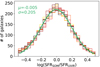 |
Fig. 5. Validation of the SOM estimates with “out-of-bag” objects. The COSMOS2020 SOM described in Sect. 3 is built again ten times, excluding every time ∼3000 galaxies randomly extracted from those with a SFRUVIR. The figure compares SFRSOM and SFRUVIR for each SOM realization (histograms of different colors). The Gaussian fit to the ensemble of distributions (green line) has mean μ = −0.005 and standard deviation σ = 0.205 dex. |
Error bars on an object-by-object basis can be provided in different ways. Hemmati et al. (2019a) proposed a Monte Carlo re-mapping of the target galaxy, each time perturbing its colors within the corresponding 1σ uncertainty; the object is scattered in nearby cells and the minimum and maximum (mass or SFR) values it reaches are used as lower and upper limits of the error bar. Speagle et al. (2019) adopt a different approach, which assigns to each cell a probability of hosting the target galaxy proportional to its χ2 (see Eq. (B.1)). We tried both methods and found that they often provide significantly different error bars. A possible explanation is the fact that (i) in the Monte Carlo we perturbed colors independently (i.e., without taking into account covariance) or (ii) the color error bars do not correspond precisely to a 68% uncertainty, resulting in a biased χ2. We preferred to invest more time exploring this issue, postponing the ascription of error bars to MSOM and SFRSOM to a future study.
4. Results
In this section, our SOM-based analysis in SXDF is compared to other methods that independently derived stellar masses and SFR for the same objects. The alternate measurements for stellar masses are produced by means of LePhare, which fits BC03 templates to SEDs that includes not only the data used in the SOM but also UV photometry from GALEX, medium- and narrow-bands in the optical, and IRAC channel 3 and 4. These estimates are originally published in Mehta et al. (2018), but we re-run LePhare to update some of its parameters to the actual configuration used for COSMOS2020 (the redshift being fixed at the same value used in Mehta et al. 2018). For the SFR comparison, we first compare to Barro et al. (2019), a study already introduced above which is restricted to the CANDELS ∼200 square arcmin area within SXDF. Like in Mehta et al. (2018), Barro et al. (2019) also exploit a set of observations larger than the 12 broadbands colors used to feed the SOM. Their study assumes the same cosmological parameters and IMF used here, but other adjustments related to Eq. (1) are required to convert their SFR estimates to a common ground. This homogenization procedure is described in Appendix A. Another set of independent estimates comes from spectroscopic data, where nebular emission lines can be used as a proxy for the SFR.
4.1. Stellar mass estimates
The stellar mass comparison (Fig. 6) shows a good agreement between MLePh and MSOM. The systematic offset between the two, measured as log(MSOM/MLePh), is < 0.02 dex. The relative scatter of 0.25 dex is nearly symmetric, with the exception of a ∼3% for which MSOM is severely underestimated (i.e., more than a factor 3). The majority of that subsample has 1.2 < zLePh < 1.8 and is located either along the borders of the grid (i.e., they suffer from “boundary effects”) or in the central area characterized by large Δ values (see Sect. 5.4).
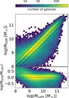 |
Fig. 6. Comparison between stellar masses obtained through standard template fitting (MLePh) and the new method presented in this work (MSOM). The figure shows the density map of 208 404 galaxies in the SXDF field with the magnitude cut at Ks < 24.2. Upper panel: a solid line marks the 1:1 relationship. Bottom panel: the logarithmic ratio log(MSOM/MLePh) is shown as a function of log(MLePh/M⊙), the solid line marks the zero offset while the two dotted lines are set at ±0.3 dex. |
At a first glance, such an agreement may seem obvious because the set of Mlabel used to derive individual masses in the SOM is built from LePhare estimates (Eq. (3)). However, there are several deviations from the SED fitting performed by LePhare that make the SOM method substantially different. First, the smaller number of photometric data points used in the latter, as emphasized above. In addition, the available “solutions” in the SOM fit are much smaller, given the limited number of cells used to describe the data manifold (6400 in total). On the contrary, the synthetic templates used by LePhare are between five and eight thousands at every fixed z step12 and over two millions in total.
We also notice that in the SOM method only the weights in the surroundings of the galaxy target are relevant for the MSOM calculation (see Eq. (6)), whereas there are no mass priors in LePhare. In the library of the latter, the BC03 galaxy models are all defined at 1 M⊙, but each of them can be rescaled to fit the observed SED. This means that each template can span the entire stellar mass range of the target pool, that is, it would be eligible to fit any observed galaxies irrespective of its mass (or other characteristics). Moreover, the choice of either using or disregarding a SOM weight for a certain galaxy is modulated by the adaptive resolution of neighboring cells, namely, the fact that in dense areas of the parameter space the SOM concentrates more weights. Another distinctive feature of the SOM, which may be regarded as an advantage or a shortcoming depending on the scientific goal, is that its collection of “empirical” weights is limited by the survey’s characteristics (e.g., its selection function). On the other hand a synthetic template library, at least theoretically, may include models of known galaxy types that are not observed in that survey (e.g., low-mass objects fainter than the detection limit), but it may also miss real objects that have not been correctly simulated as templates. Given these differences, the small fraction of catastrophic errors and the overall tight 1:1 correlation are a remarkable confirmation of the effectiveness of the SOM method.
4.2. SFR estimates
First, we compared the SOM estimates to the SFRUVIR ones from Barro et al. (2019). The authors only analyze CANDELS-UDS, which is about one-twentieth of the whole SXDF area. As an additional restriction we select only the CANDELS galaxies with UV-to-FIR data available. Also given the SOM cut at z < 1.8 and Ks < 24.23, there are only 608 galaxies in common with Barro et al. (2019). For AGN contamination, we consider the classification from Mehta et al. (2018) which is similar to the one applied to the COSMOS2020 training sample. We also discard sources with discrepant redshift estimates, that is, the absolute value of the difference between zLePh and the photometric redshift from Barro et al. (2019) is greater than 0.3(1 + zLePh). The 608 sources are plotted in the left panel of Fig. 7, showing a fairly good agreement: the −0.05 dex offset in log(SFRSOM/SFRUVIR) is comparable with the −0.03 dex initially found in the CANDELS-COSMOS comparison13. The SFR scatter (i.e., the standard deviation of the distribution in the left panel of Fig. 7) is 0.28 dex, comparable to that of the stellar mass distribution. The log(SFRSOM/SFRUVIR) histogram (inset in the left panel of Fig. 7) features a tail of a few objects that the SOM severely underestimates with respect to Barro et al. (2019), many of them being very dusty (AV > 2 mag) according to the latter. Dust correction is indeed one of the major parameters responsible for this kind of discrepancy, as discussed, for instance, in Speagle et al. (2014).
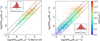 |
Fig. 7. Quality assessments of the SFRSOM estimates using independent measurements from the literature as “ground truth”. Left panel: comparison between SFRSOM and the template-based estimates from Barro et al. (2019, SFRUVIR) for 608 galaxies at z < 1.8 in the SXDF-CANDELS area (colored dots). For sake of consistency, the Barro et al. (2019) estimates are converted to the same reference system of Ilbert et al. (2015), since the latter has also been used to calibrate the SOM method (see Appendix A). Right panel: comparison to another star formation estimator, that is, Hα nebular emission line. In this case the comparison is performed in COSMOS, for 3718 galaxies (colored dots). In both panels, the color palette from violet to red indicates the stellar mass of each galaxy according to the SOM method; the solid line is the 1:1 relation from which two dashed lines are set at a distance of ±0.3 dex. Each panel also includes an inset that quantifies the dispersion between SFRSOM and the alternate estimate (red histogram); the vertical dotted line marks the median offset, which is −0.05 dex for log(SFRSOM/SFRUVIR) and 0.07 dex for log(SFRSOM/SFRUVIR). |
Another star formation proxy that can be used for comparison is the luminosity of Hα nebular emission line (LHα). We assume SFRHα = 2.1 × 10⁻⁸ × LHα (Kennicutt 1998) after correcting for dust attenuation in the host galaxy. The formula for such a correction is the same as in Kashino et al. (2013), based on the stellar color excess E(B − V) parametrized by LePhare while measuring the photometric redshift.
It is more convenient to perform this test in the COSMOS field instead of SXDF, because we have access to an unparalleled amount of spectroscopic data in the former. The most relevant surveys to our purposes are zCOSMOS (Lilly et al. 1996), 3DHST (Brammer et al. 2012; Momcheva et al. 2016), KROSS (Harrison et al. 2017), and FMOS (Kashino et al. 2019), targeting different galaxy types from z ∼ 0.1 up to 1.7. They have been selected and merged into a single spectroscopic catalog in Saito et al. (2020). Because of the overlap between these line emitters and the SOM calibration sample, we prefer to compare SFRHα versus SFRSOM for the out-of-bag galaxies of the SOM bootstrap test (see Sect. 3.3 and Fig. 5). Assuming SFRHα to be the “ground truth”, the comparison is a further validation of the SFRSOM estimates, presented in the right panel of Fig. 7. The resulting scatter (0.4 dex) and systematics (+0.07 dex) are relatively contained considering the differences between the two methods, especially the shorter time scale of star formation (on the order of 10 Myr) probed by LHα. We also note that the 0.07 dex offset shown in the figure is mainly due to the most massive galaxies, which may have a biased SFRHα: in fact, their dust content is usually high and susceptible to be underestimated by LePhare, whose templates are limited to E(B − V)≤0.7 and may not assume the correct extinction law (Ilbert et al. 2010; Walcher et al. 2011). Moreover, in (local) massive galaxies, nebular extinction often adds a greater contribution to stellar dust extinction (van der Giessen et al. 2022) and BC03 models do not take this into account.
4.3. Main sequence of star-forming galaxies
With the SXDF2018 photometric redshifts, stellar masses, and SFRs obtained through the SOM we can trace the main sequence of star-forming galaxies (MS) and its evolution as a function of cosmic time. The SFRSOM versus MSOM plane at different redshifts is shown in Fig. 8, where we choose the following bins in order to ensure homogeneous time intervals: 0.3 < z ≤ 0.4, 0.5 < z ≤ 0.7, 0.9 < z ≤ 1.1, 1.4 < z ≤ 1.8. The four bins are centered around median redshifts of z = 0.3, 0.6, 1.0, and 1.5 corresponding to t = 9.8, 7.7, 5.7, and 4.2 Gyr after the Big Bang. The time step between the last two bins is the only one shorter than 2 Gyr because of the z < 1.8 upper limit imposed by MIPS. Galaxies at z ≲ 0.2 are not included since COSMOS probes a small cosmic volume below that redshift, thus losing most of its statistical power. A more conventional binning is used later in this section for the purpose of making a compare with the literature. Similarly to the χ2 cut applied in many template-fitting studies (see e.g., Bowler et al. 2015), we removef the “bad fit” objects having Δ > 5. This threshold rules out nearly 1% of the galaxies whose SED is not well represented by the weight of their own cell.
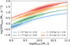 |
Fig. 8. Evolution of the main sequence of star forming galaxies resulting from the SOM-based measurement of the SXDF2018 catalog. Redshift bins are chosen to correspond to four time steps separated by ∼2 Gyr, whose color is indicated in the legend along with median redshift and cosmic age. In each bin, the main sequence is identified as the most prominent overdensity in the SFRSOM − MSOM plane (shaded areas representing density contours). Each overdensity peak is fit by Eq. (8) either independently (solid lines) or simultaneously at all t (dashed lines). |
To locate the MS we apply a procedure inspired by the MS definition in Renzini & Peng (2015). In that study14, the MS naturally emerges as a peak in the surface formed by all the galaxies in the 3D space SFR versus mass verus number of objects, without any a priori separation between star forming and quiescent. In the Renzini & Peng (2015) framework the MS core is the “ridge” of such a 3D peak, a line that is stable whether or not the data set includes, for instance, post-starburst galaxies exiting the MS. A similar approach, not requiring a preselection of the star-forming sample, was recently proposed in Leja et al. (2021). The SOM method, however, is not entirely free from selection effects because galaxies falling far from the labeled cells do not obtain any SFRSOM estimate by construction. Irrespective of that potential bias, which will be discussed in Sect. 5.2, the SXDF2018 sample includes a wide range of galaxies, from starbursts above the MS to galaxies with low specific star formation rates.
To identify the ridge of the star forming sequence we apply the following procedure in every zSOM bin. First, a Gaussian kernel density estimator15 is used to build a probability distribution map of SXDF2018 objects in the log(SFRSOM) versus log(MSOM) space. Each map is shown in Fig. 8 with isodensity contours of different colors. Resampling them with a grid of points equally spaced by 0.05 dex we find the ridge of the density peak (i.e., the “backbone” of the MS) and track its evolution over ∼6 Gyr. The ridges in the four redshift bins are interpolated by the same function used in Schreiber et al. (2015):
![Mathematical equation: $$ \begin{aligned} { y} = m - m_0 + a_0 r - a_1 [\mathrm{max} (0,m-m_1-a_2r)]^2, \end{aligned} $$](/articles/aa/full_html/2022/09/aa43249-22/aa43249-22-eq8.gif) (8)
(8)
where r ≡ log(1 + z), m is the logarithmic stellar mass in units of 109 M⊙, and y is the logarithmic SFR in M⊙ yr−1. The other five parameters (m0, m1, a0, a1, a2) are obtained via nonlinear least-square minimization using a trust region reflective algorithm16. The best-fit values for the free parameters, listed in Table 2, result into the solid lines shown in Fig. 8. We also fit the four sequences together (dashed lines) obtaining the following parameters: (m0, m1, a0, a1, a2)=(0.75 ± 0.04, 0.0 ± 0.2, 3.2 ± 0.2, 0.17 ± 0.04, 0.0 ± 0.5). The terms m1 and a2 being consistent with zero indicates that there is no need for second-order corrections to describe the MS turnover at high masses. This is the major distinction with respect to the MS of Schreiber et al. (2015), where the bending is more pronounced. In fact, thanks to the stacking of Herschel images, (Schreiber et al. 2015) gain sensitivity to measure also galaxies with very low sSFR. The best-fit parameters they find are (m0, m1, a0, a1, a2)=(0.5 ± 0.07, 0.36 ± 0.03, 1.5 ± 0.15, 0.3 ± 0.08, 2.5 ± 0.06). For sake of completeness, we also try a linear interpolation using the function y = (α0t + α1)log(M/M⊙)+(β0t + β1) as done in Speagle et al. (2014, in Eq. (17)), but the goodness of fit is inferior to Eq. (8) and, therefore, it is not shown in the figure.
We also select from the literature some of the most relevant studies that have measured the MS between z = 0 and 2, namely, Whitaker et al. (2014), Schreiber et al. (2015), Ilbert et al. (2015), Barro et al. (2019), Leslie et al. (2020). To estimate galaxy SFRs those authors use different methods, all based on FIR data with the exception of Leslie et al. (2020) performing a radio analysis. Two of these studies deal with individual sources only (Whitaker et al. 2014; Barro et al. 2019) while the other two include undetected galaxies by stacking either 3 GHz VLA (Leslie et al. 2020) or Herschel (Schreiber et al. 2015) images. Ilbert et al. (2015) derived the MS from MIPS-detected galaxies but in an indirect way, through the SFR function. All the selected studies identify the MS locus by binning their sample in stellar mass and then computing the median SFR in each bin. Although such an approach is suboptimal from a mathematical point of view (Steinhardt & Jermyn 2018), we decided nonetheless to proceed in the same way as the other authors have done in order to maintain coherence17.
The SOM results are in good agreements with the other MS measurements (Fig. 9) showing that SFRSOM and MSOM estimates are accurate not only when evaluated separately. Overall, the differences between our MS and previous results are comparable with the differences between them, and smaller than the 1σ error bars that we defined as the 16th–84th percentile range in each mass bin. There are, however, two visible systematics, at both extremes of the probed mass range, which are worth noticing. At the low-mass end, our median points slightly deviate from the linear extrapolation of the MS. This is related to a sample incompleteness in those mass bins and a consequent skewness of the SFR distribution towards higher values. The incompleteness is shown in Fig. 9 by white and orange filled circles, marking bins in which the fraction of galaxies with a defined SFRSOM drops below 50 and 70%, respectively18. The other systematic effect concerns the most massive bin, which at z > 1 is always located above the other studies (although within ∼1σ from them, see Fig. 9). In general, our median SFRs do not show the high-mass turnover observed in Ilbert et al. (2015), Lee et al. (2015), and subsequent studies (see discussion in Sect. 5.2). Besides that, the overall slope and redshift evolution of our MS agree with previous work confirming the reliability of the SOM method.
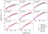 |
Fig. 9. Redshift evolution of the MS of star forming galaxies (see Sect. 4.3) as determined in the present work (red circles), Ilbert et al. (2015, blue diamonds), Barro et al. (2019, pink squares), Whitaker et al. (2014, blue dotted line), Schreiber et al. (2015, brown solid line), and Leslie et al. (2020, green dashed line). Our estimates stop at the z-dependent threshold for stellar mass completeness defined in Weaver et al. (2022). Their error bars are the 16th–84th percentile range and each symbol is filled with a shade of red according to the completeness of the given mass bin; in particular, dark red symbols represent > 90% completeness, orange between 60 and 80%, while white-filled circles have ≲50% completeness (see Sect. 5.2). Results from the literature are shown only when the median redshift of the given study is sufficiently close to ours (which is indicated in the upper-left corner of each panel); the same measure may be repeated in more than one panel: for example, the MS of Barro et al. (2019) at 0.5 < z < 1 has a median redshift ⟨z⟩=0.8 and it is compared to our data both at 0.6 < z < 0.8 and 0.8 < z < 1.0. |
5. Discussion
5.1. SOM-based estimates versus synthetic templates
To assess any improvement the SOM may provide over standard template fitting, the latter has to be compared to reference estimates (Barro et al. 2019) as it has been done with SFRSOM (Sect. 4.2). Figure 10 shows such a test in the overlapping part of the SXDF field (see Appendix B for COSMOS). When exactly the same 12-band photometry is used (cf. Table 1), the scatter in log(SFRLePh/SFRUVIR) is significantly larger than what found for the SOM-based method (cyan circles in Fig. 10). The distribution becomes narrower, and less skewed, if additional colors (25 filters in total) are provided as input to LePhare (blue squares in Fig. 10). Either way, the fit is performed without data points in the FIR regime. For the 12-band fitting we run LePhare using the same version and set-up of COSMOS2020, while the fit to the extended photometry comes from Mehta et al. (2018). Therefore, the latter estimates not only include ancillary data (medium- and narrow-band filters from Subaru and VISTA telescopes) but are also derived with a configuration of LePhare that is optimized for SXDF2018. However, even in that case, the template-based estimates are less precise than SFRSOM.
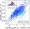 |
Fig. 10. Comparison between Barro et al. (2019) and LePhare using the same sample of 608 galaxies also shown in the left panel of Fig. 7. The same BC03 library is fit by LePhare to the full photometric baseline available in the SXDF2018 catalog (filled blue circles) and to the 12 filters only used in the SOM method (open cyan circles). Same colors are used in the inset for the histograms showing the respective log(SFRLePh/SFRUVIR) distributions; the log(SFRSOM/SFRUVIR) distribution (red histogram, same as the inset in the left panel of Fig. 7) is also included as reference. |
The effective performance of our method is mainly due to the empirical collection of galaxy prototypes that the SOM creates during training (see also the “phenotypes” in Sánchez & Bernstein 2019). Similarly to eigenvectors in a principal component analysis, the SOM weights are adapted to the observed sample so that “by construction” their colors represent realistic SEDs, to which physical properties are attached. These properties can be derived from scaling relations or other empirical recipes, which, despite their underlying assumptions, offer a complementary approach to the use of stellar population synthesis models.
In standard template fitting, the library is generated from theoretical models that might not be an accurate description of the observed targets – or even of their parent populations – especially regarding their star formation scenarios. In fact, many template libraries (including the one in Weaver et al. 2022) are built by using a simplistic SFH parametrization (exponential-τ and delayed-τ models, see Ilbert et al. 2013) with a limited number of time steps, which may be inadequate, for instance, for starburst galaxies (Pacifici et al. 2013). Moreover, the physical parameter space is sampled by a coarse grid of stellar metallicity and E(B − V) values, and there are limited options to add nebular emission line contamination (Pacifici et al. 2015; Yuan et al. 2019). Part of the parameter space covered by the models might have no correspondence in the observed universe (see the discussion in Marchesini et al. 2010; Muzzin et al. 2013 concerning dusty, passive galaxy templates). Moreover, the grid discretization may introduce severe biases, as investigated in Mitchell et al. (2013). Besides these approximations, the simplistic modelling of dust attenuation plays a major role (Chevallard et al. 2013; Chevallard & Charlot 2016; Laigle et al. 2019).
To better visualize these concepts, we derive observed-frame colors for the BC03 templates in the LePhare library, shifting them from z = 0.2 to 1.8 with a linear increment of Δz = 0.01. Once projected on the COSMOS2020 SOM, these templates occupy only a fraction of the grid (Fig. 11) even after perturbing their photometry with Gaussian-shaped noise (0.05 mag standard deviation for every band). Their distribution (number of templates per cell) is very different compared to that of COSMOS2020 galaxies (cf. Fig. 11 and the left-hand panel of Fig. 2). Such a tension is not surprising because the sample of BC03 colors is built with a flat redshift distribution and no differentiation in the abundance of galaxy types. This has an impact on the whole SED fitting process comparable to the bias from missing templates (empty cells in Fig. 11). Especially in codes like LePhare, which do not take into account prior probabilities, if a “family” of (z, M, SFR) models is over- or under-represented in the library then the output quantities will be biased too.
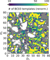 |
Fig. 11. BC03 templates from the LePhare library projected into the SOM. The templates are shifted from z = 0.2 to 1.8 with steps of Δz = 0.01, and perturbed with Gaussian noise to mimic real photometry. The SOM is color coded to show their cell occupation, renormalized to the number density of COSMOS2020 galaxies to make this figure directly comparable with the left-hand panel of Fig. 2. |
The severity of this last issue shall decrease in future studies owing to the expected improvement of telescope surveys, since a higher photometric quality shall result in more robust likelihood functions. In such a scenario, the likelihood would drive the SED solution to eventually make the code less sensitive to the models’ priors, but if a model were completely missing from the library (not just over- or underrepresented), then the problem discussed above would persist in spite of the increased quality of the input data.
A treatment of probability distribution functions including probability priors is presented in Benítez (2000) and Tanaka (2015) for redshift measurements only. The same Bayesian formalism is also the foundation of state-of-the-art SED fitting codes to estimate physical properties, with notable examples including BAGPIPES19 and Prospector20. Another distinctive feature of these codes is the capability of using SFHs in flexible bins of time (often designated as “non-parametric”, see Leja et al. 2019b) or to include a large variety of SFHs from cosmological simulations (as in BEAGLE, see Chevallard & Charlot 2016). Also, the implementation of parametric SFHs has reached a level of complexity higher than the previous generation of software (see Carnall et al. 2019). This is however achieved at the expenses of computational speed. In that regard, the advantage of SOM is well illustrated in Hemmati et al. (2019a): the time to process 107 objects is less than 0.3 CPU hours, while a typical Bayesian fitting run (e.g., Mehta et al. 2021) would take a similar amount of time for a single object (V. Mehta, priv. comm.). Such a trade-off may dramatically change in the future, as cheaper machines (i.e., the possibility to rent or buy more CPU time) and more efficient Bayesian methods become available. A promising example in this direction is the SED inference method proposed by Hahn & Melchior (2022) that employs simulation-trained neural networks to accelerate the estimate posterior probability distributions at the pace of 1 s per galaxy (which despite the dramatic improvement would still exceed the 0.3 CPU hours of the SOM to analyze our sample).
In recent work, the SFRs derived from the Bayesian codes mentioned above have been compared with other estimators. In Carnall et al. (2019) galaxies in the GAMA survey (Baldry et al. 2018) are analyzed with BAGPIPES and then compared to SFR measurements based on Hα flux, showing a large scatter (see their Fig. 9) and a mass-dependent offset due to the fact the Hα tracer is sensitive to more recent star formation episodes. The test with GAMA galaxies is performed at z < 0.1, fitting bands up to IRAC channel 4. These differences stand in the way of a straightforward comparison with our SFRHα test (Fig. 7, right panel) which, however, shows more consistency even though it has been performed over a larger z range and without the use of channel 3 and 4.
Another recent study (Leja et al. 2021) thoroughly inspects physical quantities inferred by means of Prospector for 3DHST and COSMOS2015 galaxies up to z ∼ 3. Unlike the present analysis, their input photometry spans from UV to 24 μm (when available) and the emission in those bands is interpreted under the assumption of energy balance (similarly to da Cunha et al. 2008). With this caveat in mind, we can compare to Leja et al. (2021) by examining the COSMOS galaxies Leja et al. (2021) have in common with our study. Among the ones with a 24 μm detection (S/N > 5) we select 790 targets that have been kept out-of-bag during the validation test in Sect. 3.3. Another 16 729 galaxies in our catalog have no 24 μm counterpart (or < 5σ), but they are matched with a source in Leja et al. (2021). For the former subsample, we find no significant systematics in log(SFRSOM/SFRProspector), along with a standard deviation of 0.3 dex that is comparable with the typical SED fitting statistical uncertainties (Fig. 12, upper panel). With respect to the objects that are not detected in MIPS, we are able to confirm the findings in Leja et al. (2021): when sSFRProspector ≳ 1010 yr−1 there is a good agreement between the two techniques, whereas below the MS, the SFRSOM values are systematically larger (Fig. 12, lower panel). The average discrepancy increases from 2× to more than 10×, as we move towards lower levels of specific star formation. Such a trend is coherent with Prospector non-parametric SFHs since their impact, compared to analytical descriptions of SFH, is more pronounced for old galaxies that have exited the MS.
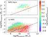 |
Fig. 12. SFR vs. M plane of COSMOS2015 galaxies (colored circles) as it results from the SED fitting performed by the Prospector code (Leja et al. 2021). Only the objects cross-correlated to COSMOS2020 (0.6″ searching radius) are shown, both those having a MIPS 24 μm counterpart (in the upper panel) and objects without FIR detection (lower panel). Each data point is color-coded according to the difference in SFR between Prospector and the SOM estimator. A dashed line at constant sSFR = 10−11 yr−1 is plotted in each panel to guide the eye. |
Another reason behind the differences among the two methods is that galaxy models in Prospector are composed of a combination of various stellar populations. Such a flexibility corresponds to a variable scaling factor in the SFR–LIR relationship, which can be adjusted on an object-by-object basis instead of the constant 𝒦 factor used to calibrate the SOM (Eq. (1)). In fact, the latter comes from studies based on simpler stellar population synthesis models. The discrepancy, however, could be removed by construction using Prospector to label the SOM instead of the procedure summarized in Sect. 2.3. This option is further discussed in Sect. 5.3.
5.2. Caveats in the SOM construction
The most entrenched limitations in the SOM method are the ones inherited from training and calibration samples. In Sect. 4, we shared the observation that many galaxies do not have an assigned SFRSOM. The lack of estimates is due to the 24 μm flux limit, which prevents the measurement of most of the low-SFR galaxies with M < 1010 M⊙, leaving several SOM cells without a SFRlabel. As a consequence, the SFR distribution in bins below 1010 M⊙ is skewed towards higher SFR values, and the observed MS departs from linearity (Fig. 9). This selection bias would affect any MS measurement derived from the COSMOS MIPS survey, irrespective of the method; with the SOM, the way data are visualized makes easier to identify this kind of issues. Incompleteness in the training sample is more difficult to quantify because it is necessary to characterize the parent population from which the sample is drawn. It is therefore challenging to establish, before starting the SOM construction, whether a certain galaxy type has not been included in the training. Template fitting does not have the same problem, since that particular galaxy type can always be incorporated in the template library; the concern in that case is how accurately that galaxy is modeled.
Another bias, more specific to the SOM method itself, is caused by the mixture of different galaxy types in the same cell. The main reason for such a contamination is the similarity of diverse SEDs after photometric errors are taken into account. This has been already shown in Speagle et al. (2019, particularly in their Figs. 3 and 4), albeit, for a five-band data set, which is more susceptible to SED degeneracy. In an ideal, noiseless universe, the SOM classification is extremely accurate, as shown in Davidzon et al. (2019) using a mock galaxy catalog from hydrodynamical simulations. Hence, the necessity of using deep, state-of-the-art data to minimize observational errors and, consequently, the scatter introduced in the SOM. Cells with a quiescent fraction of 0.25 < fQ < 0.75 (5% of the entire grid, see Fig. 4) are another example of the SED mixing, indicating that some galaxies with different NUV − r, r − Ks colors are located together inside the same cell. This bias may affect more seriously those calibrations relying on smaller samples, like SFR in the present study. In cells occupied only by a handful of MIPS galaxies, even a single interloper may have a strong impact on the resulting SFRlabel. One way to find them is to look at some property that is expected to be similar for all galaxies in the cell (e.g., their sSFR). If the inspected object is an (e.g., 2σ) outlier of the distribution, then it can be flagged as a potential interloper. The suggested approach is only one of the possible solutions and it does not work in some cases, for instance, in cells containing only one or two MIPS galaxies. Nonetheless, we test it by re-calibrating the SOM using sigma-clipped SFRUVIR distributions. This effectively removes 2σ outliers in the cells where sigma clipping is feasible. Since the general results of the analysis do not change, we conclude that contamination bias does not have a strong impact overall.
Instead of relying on galaxy physical properties, like in the example above, we can find catastrophic errors in the SOM classification by inspecting galaxies with suspiciously large Δ or χ2 distance (Eqs. (2) and (B.1), respectively) as done in Sect. 4.3. Another way to mark unreliable SFRSOM estimates is according to the number of cells contributing to Eq. (7): for some galaxies not all the N neighbors may be labeled, potentially introducing a bias. Such a bias, if present, must be of second order because removing objects for which only one or two of the five neighbor cells have SFRlabel defined, the MS locus does not change; the only detectable change is a reduction in the error bars of Fig. 9.
Certain sub-samples of galaxies are, however, affected by an ambiguous SOM classification besides the obvious interloper cases. This is the case of the trend at the high-mass end of the MS, already highlighted in Sect. 4.3. Since there is no clear-cut separation between the star-forming and quiescent population in the SOM, we impose a threshold (fQ < 0.5) that is somewhat arbitrary. Figure 13 illustrates the issue at 0.6 < z < 0.8: massive galaxies with intermediate to low star formation, responsible for the MS turnover at ∼5 × 10¹⁰ M⊙, are excluded by the fQ < 0.5 criterion. A less conservative constraint (sSFR > 10−11 yr−1) does not remove those galaxies and would better identify the MS turnover, becoming more in agreement with the MS determined by the “selection-free” definition of Renzini & Peng (2015, see Sect. 4.3). The same is observed in the other redshift bins. Figure 13 also shows the general systematics induced by using the median SFR in bins of mass: they locate the center of the MS slightly below the locus traced by the highest density in galaxy number density.
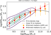 |
Fig. 13. Solid lines show the contour density map for the distribution of SXDF2018 galaxies in the SFR–M diagram; this is fit by Eq. (8) as described in Sect. 4.3 (dashed line). Filled circles are SFR median in running bins of galaxies with SFRSOM/MSOM > 10−11 yr−1 (orange symbols) and fQ < 0.5 (red). In both cases, error bars are calculated with the 16th–84th percentile difference. The red circles are interpolated by a linear function (dotted line). |
5.3. Calibration with other tracers
The estimates used as reference in Sect. 2.3 are not the only option for calibrating our method. Relying on the same optical-to-FIR data, we can use alternate fitting codes (e.g., Prospector) instead of LePhare. Besides that, owing to the wealth of ancillary data in COSMOS, other proxies for stellar mass and star formation can provide Mlabel and SFRlabel. This is particularly evident for the latter, which can be derived, for instance, from Hα nebular emission or by the radio continuum. Other possibilities, such as the 21 cm atomic hydrogen or sub-mm molecular gas transitions, are not included in the present discussion for sake of simplicity and we address the reader to Kennicutt & Evans (2012) for an exhaustive bibliography on the various star formation tracers. Our goal in the present section is not to repeat the analysis with another sets of MSOM, SFRSOM estimates – but, rather, to show the capacity of different calibration samples to fill the SOM grid.
A technique for deriving SFRHα has been presented in Sect. 4.2. Radio continuum emission is also correlated with galaxy star formation (Condon 1992), but we do not calculate SFRradio here since we aim at discussing the availability of data rather than the final estimates. The latest, publicly available21 radio data for almost the entire COSMOS field come from interferometry in the 3 GHz band with the ESO Very Large Array (Smolčić et al. 2017). Instead of extracting individual sources, as done with both MIPS and spectroscopic tracers, we could stack 3 GHz map cutouts centered at the position of SOM galaxies belonging to the same cell. This is the procedure adopted by Leslie et al. (2020), which is similar to the 1.4 GHz stacking described in Karim et al. (2011).
Figure 14 shows the coverage of potential calibrations with either Hα or radio stacking, along with the actual FIR-based calibration already presented in Fig. 4 (bottom-left panel). We highlight only the cells that would benefit from a high-confidence calibration, namely, those containing at least one galaxy with Hα flux > 2 × 10⁻¹⁷ erg s−1 cm−2, or with S/N > 3 in the 3 GHz median stack. The figure of merit for radio stacking is done by following the recipe (size of the cutouts, calculation of median flux, etc.) in Leslie et al. (2020).
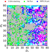 |
Fig. 14. Different calibration samples that may be used to label SFR on the SOM. Cells containing galaxies from the original MIPS sample (cf. Fig. 4) are colored in blue; cells containing spectroscopic galaxies with an Hα measurement and radio galaxies with a 3 GHz stacking S/N > 5 are colored in green and red respectively. Colors combine by following the standard RGB rules, e.g. a cell that can be calibrated by both MIPS and Hα (MIPS and radio) is colored in cyan (magenta). A handful of yellow pixels are cells that can be calibrated by only radio stacking and Hα, while white pixels are cells in which all the three star formation tracers are available. As the discussion in the main text is only about coverage and not the actual SFRlabel values, these are not shown in the present figure. |
The most evident feature of Fig. 14 is the additional coverage provided by spectroscopic data, which gives us the capability of labeling 735 cells missed by the 24 μm calibration. Most of them are in the area populated by low-mass galaxies because of the surveys’ selection function targeting many emitters with MLePh ≃ 109 M⊙. This shows how spectroscopic line detection can be complementary to FIR imaging. The figure of merit is expected to improve after next-generation spectrographs will start operations. For example, Hα is inside the wavelength range of the Multi-Object Optical and Near-infrared Spectrograph (MOONS, Cirasuolo et al. 2014; Taylor et al. 2018) in low-resolution mode from z ∼ 0 to 1.7, with Hβ (pivotal for dust correction) entering at z ∼ 0.3. The sensitivity and multiplex capability of the instrument22 shall enable a more exhaustive labeling of the SOM grid (see discussion in Davidzon et al. 2019). Also, the grism spectrograph on board of Euclid23 could be instrumental not only for filling the empty cells but also to dramatically increase the statistics: between 32 000 and 48 000 galaxies per square degree are expected to be observed at 0.40 < z < 1.8 with an Hα flux > 5 × 10⁻¹⁷ erg s−1 cm−2 (Pozzetti et al. 2016).
The third tracer, based on 3 GHz stacking, provides an SFRlabel for 510 cells, corresponds to ∼20% of the area actually sampled by previous calibrations. Very few cells (red pixels in Fig. 14) are newly labeled by the radio sample, partly due to the conservative S/N > 5 cut we imposed: if instead we also allow stacked images with 3 < S/N < 5, then the number of SOM cell probed by radio data nearly doubles. However, even in that case, the expansion with respect to the original MIPS calibration would be limited (only 65 additional SFRlabel) due to the FIR-radio correlation and its strong dependency on stellar mass (Delvecchio et al. 2021). Despite such a marginal expansion, it is still useful to have various tracers superimposed on the SOM for a better understanding of the galaxy parameter space. For example, a difference between multiple SFRlabel values in the same cell may help identify galaxy classes with rapidly varying SFH, leveraging the fact that those star formation tracers probe different time scales (which can be taken into account as in Sparre et al. 2015).
In Leslie et al. (2020), the stacking technique is instrumental to probe the SFR–M plane beyond the boundaries of the original Smolčić et al. (2017) sample, which is made by individual VLA sources whose counterparts are mostly brighter than 22.5 mag in IRAC channels 1 and 2. Moreover, the choice of adaptive binning allows the authors to always gather several hundreds of objects. In the finer grid of the SOM, galaxies that in Leslie et al. (2020) belonged to a single (z, M) bin are now spread over several cells, “diluting” the stacking signal. One route to solving this problem involves the use of all SOM cells, each one with an occupation probability weight (as in Speagle et al. 2019), instead of assigning the target galaxy to its best-fit (but low-S/N) cell only.
As an aside, we notice that a stacking strategy would be more beneficial for the SFRUVIR calibration. The MIPS sample used in Sect. 3.2 was pre-selected at S/N > 5 in the 24 μm band. A preliminary inspection of sources below that threshold suggests that the number of labeled cells may increase by ∼30% (compared to Fig. 4) by using median SFRs from 24 μm stacking (calculated as in Magdis et al. 2010).
5.4. Soundness checks using SOM
None of the three tracers we considered are able to fill the central area of the SOM (around coordinates D1, D2 = 50, 40), where the average intra-cell distance is particularly large (Fig. 2, middle panel). This is another use of the SOM as a diagnostic for peculiar SEDs (see also Hovis-Afflerbach et al. 2021, where they apply dimensionality reduction to isolate catastrophic redshift errors). The bottom panel of Fig. 15 illustrates this point through the galaxy sample inside one of those problematic cells (the one with coordinates D1, D2 = 46, 34). The sample includes 56 objects at z ∼ 1.2 with similar colors. When the SEDs are superimposed to their LePhare best-fit templates, we observe that the UltraVISTA H band is systematically below the flux predicted by LePhare (see lower panel of Fig. 15). The corresponding photometric uncertainty is also significantly larger than the other UltraVISTA bands, always resulting in a S/N smaller than 2. Interestingly, Chartab et al. (in prep.) also reached the same conclusion by analyzing H-band photometry with a different ML technique, where these objects had escaped standard reliability checks in Weaver et al. (2022).
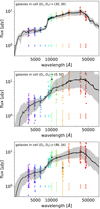 |
Fig. 15. Inspection of three SOM cells with coordinates (D1, D2)=[(30, 30),(0, 50),(46, 34)] on the 80 × 80 gird. The first cell (upper panel) has been randomly selected among those with a small galaxy-weight distance Δ (cf. Fig. 2) while the middle and lower panels display two cells located in areas with large Δ values, to provide an insight on SOM shortcomings (see Sect. 5.4). The number of galaxies in these cells is respectively 16, 39, 56. In each panel, the solid line is the median of the BC03 spectral models providing the best fit to each COSMOS2020 galaxy in the LePhare analysis; before calculating the median, all the BC03 spectra (which include only the stellar component, not the nebular emission) have been rescaled to match 22.5 mag in the i band. Such a rescaling also makes easier to compare spectral shapes from the different panels. The gray shaded area encloses the 16th and 84th percentiles of their distribution. The y-axis range in the upper panel is shorter to zoom in the tight 16th–84th dispersion, which would be barely visible otherwise. Filled circles represent the observed photometry, color-coded for the different bands (see legend); for sake of clarity they have been horizontally shifted from the central wavelength of their band by a random offset within ±3%. In the bottom part of each panel we report the average error bars in the same color of their corresponding photometric band. Black crosses are the fluxes that would result from the cell’s weight after training. All symbols are renormalized to the reference i = 22.5 mag. |
Another problematic region according to Fig. 2 is the vertical stripe of cells with D1 = 0 and 48 < D2 < 56, from which we randomly select (D1, D2)=(0, 50) for inspection (middle panel of Fig. 15). Galaxy SEDs inside that cell have a much larger dispersion than non-pathological cells (as the one displayed in the upper panel of Fig. 15 for comparison). Despite the scatter, these objects share a common characteristic, namely, an extremely red yHSC − YVISTA color24 and a blue YVISTA − JVISTA. That color excess can be attributed to nebular emission line contamination in the YVISTA band. Indeed, galaxies in (D1, D2)=(0, 50) are concentrated around two redshifts: z ∼ 1.15 and z ∼ 1.7, which approximately correspond to a Y-band flux enhancement due to Hβ (λ4863) and O[II] (λλ3727, 3729) respectively. Hence, the SOM diagnostic power can serve at the same time to identify peculiar galaxy types like strong line emitters, but also to reveal technical issues such as photometric redshift degeneracy.
6. Summary and conclusions
Compared to the body of work focused on ML methods to measure galaxy redshifts, little progress has been made with respect to other physical parameters, which are equally important in galaxy evolution studies. Here, we continue the investigations presented in Masters et al. (2015), Hemmati et al. (2019a), and Davidzon et al. (2019) to the point where we are now able to exploit an unsupervised ML algorithm such as the SOM to simultaneously derive galaxy redshift, stellar mass, and SFR. This particular use of the SOM has already been described in Davidzon et al. (2019), but so far has been applied only on mock galaxy catalogs that, despite an advanced level of realism, cannot replace the complexity of a test with actual observations.
To this purpose, in the present work, we used the new COSMOS2020 galaxy catalog (Weaver et al. 2022) up to z = 1.8, together with the rich archive of complementary data available for the COSMOS field. Not only the quality, but also the large size of COSMOS observations make them an ideal training sample for the SOM. In our method, after the SOM dimensionality reduction created a grid of 80 × 80 cells, we labeled as many cells as possible with reference values of z, M, and SFR. These values are derived by means of ancillary data, in particular MIPS 24 μm from the S-COSMOS survey to constrain galaxy star formation. Once the SOM was calibrated, we projected other galaxies onto the grid, obtaining an estimate of their zSOM, MSOM, and SFRSOM depending on the cell to which each target has been associated. We used SXDF galaxies, but any other galaxy sample can be measured as long as the targets have the requisite features (in this case, broadband colors) to be projected into the COSMOS-calibrated SOM. In our case, we also assumed photometric redshift are known in advance to preselect galaxies below z < 1.8. This requirement can be disregarded, as the SOM proved to be efficient for redshift measurement too (Masters et al. 2015). However, the other techniques also fix the redshift of their targets before measuring the other physical parameters, therefore we did the same here for sake of comparison.
The SOM is made by a fixed number of cells, each one representing a specific combination of broadband colors (i.e., a galaxy SED prototype). The galaxy properties in output are not strongly discretized because they result from averaging several cells (Eqs. (6) and (7)). Nevertheless, the SOM resolving power is lower than other ML methods (in particular deep neural networks, see Simet et al. 2021) that describe physical parameters with continuous functions. The SOM “gridding effects”, however, are counter-balanced by the advantage of building such a grid in an unsupervised fashion, and the flexibility of assigning different labels to it a posteriori. As an aside, we note that other methods such as variational autoencoders (see Cheng et al. 2021, for an application in the astronomical domain) may represent a synthesis between the two approaches by offering both an unsupervised (or semi-supervised) training and a regression analysis with continuous functions.
We assessed the reliability of our procedure both by way of comparisons to independent estimates and by means of a bootstrap technique (i.e., out-of-bag targets from our COSMOS sample). Most notably the galaxy SFR, generally difficult to recover from optical-NIR fitting, can be measured with good precision (< 0.3 dex scatter, see Figs. 5 and 7) and is consistent with SFR indicators based on FIR (only 0.05 dex offset from Barro et al. 2019); even though in our SOM method, the input photometry stops at IRAC channel 2. We also found a good agreement between the SOM main sequence of star formation and other MS studies from the literature, an indication that the (zSOM, MSOM, SFRSOM) estimates provided by the SOM are simultaneously accurate for most of the targeted objects.
The computation of physical parameters for 208 404 SXDF galaxies took about 0.1 CPU hours. In addition to the computational speed our method offers, other advantages shall be emphasized:
The quality of SFRSOM estimates is better than the results obtained with LePhare, when compared to SFR values independently measured from UV-to-FIR photometry (Barro et al. 2019). Concerning stellar mass estimates, we found that MSOM and MLePh are in overall good agreement; small discrepancies between the two could not be solved because of the lack of a third set of M estimates to be used as “ground truth”. Without advocating that LePhare (or template fitting in general) should be superseded by the novel method, our study demonstrates the benefits of a dual approach with ML and standard template fitting working in a complementary fashion. Indeed, as LePhare was instrumental in preliminary tests on the SOM (here, but also e.g. in Hemmati et al. 2019b) the latter can help to better understand caveats and limitations in template fitting (Sect. 5.1). The key factor making our method competitive with respect to other state-of-the-art fitting codes is that it does not rely on the traditional library of synthetic templates. Such a library can be biased by the theoretical modeling assumptions (stellar population synthesis, dust prescriptions, etc.) whereas this new fitting procedure is more data-driven, based on a set of galaxy prototypes coming from the SOM classification of observed SEDs (i.e., the cells and their weights).
The robust performance of SOM does not imply that its outcome is bias-free, that is, the systematics in the training sample may propagate to the target galaxy estimates and also the SOM labels have underlying assumptions (see e.g., Eq. (1) for producing SFRlabel). However, the 2D rendering of the SOM put us in a convenient position to solve the problem, as it allows an effective visual inspection of the parameter space. Section 5.4 showed an example of such application, where we flag suspicious cells according to the average galaxy-weight distance inside them. We were able to identify not only issues due to corrupted photometry, but also galaxy types whose SED is intrinsically peculiar (e.g., because of nebular emission contamination).
Moreover, a deeper insight into the galaxy parameter space may result from the combination of multiple calibration samples. In fact, the labels used in the present analysis are not the only option in COSMOS. In Sect. 5.3 we discussed two alternatives to SFRUVIR, since the star formation labels can also be derived from either direct spectroscopic measurements (SFRHα) or VLA 3 GHz image stacking (SFRradio). Having more than one tracer helps, at least to some extent, to calibrate a larger fraction of the SOM grid, but the most important advantage is the overlap of the different tracers: in a cell with multiple layers of physical information, any similarity (or tension) between them is informative about the galaxy population inside that cell.
While discussing multiple calibration samples, we also take note of the role that next-generation spectrographs such as MOONS or the Prime Focus Spectrograph (PFS, Takada et al. 2014) will play in the near future. With those facilities, an ambitious programme such as the Complete Calibration of the Color-Redshift Relation (C3R2, Masters et al. 2017) may extend its scope to include the calibration of stellar mass and SFR over the entire area of the SOM grid. Nonetheless, 24 μm calibration shall remain a compelling option as the Mid-IR Instrument (MIRI25) on board James Webb Space Telescope will supersede MIPS images, also offering a choice among more broadbands (four of them between 15 and 25 μm). The field of view of MIRI is only 74″ × 113″, but in spite of that it should be possible to assemble a calibration sample of comparable size to the COSMOS one. In fact, owing to the small cosmic variance of independent line of sights (Moster et al. 2011), a hundred of well-separated pointings should be sufficient (see Trenti et al. 2011, for a similar strategy with HST).
Irrespective of the preferred calibration strategy, the present work is intended as a blueprint to develop ML-based software for upcoming large-area photometric surveys. Scanning a few thousands square degrees (as planned by the Euclid mission) or even the entire sky (like the Rubin Observatory), those surveys will decrease dramatically the (already small) ratio between well-characterized spectroscopic galaxies and objects only described by their broadband colors. In the SOM, the former ones would only be needed for a training sample, proportionally much smaller than the number of targets. Therefore, with modest modifications, our method can be implemented, that is, in the Euclid pipeline, deriving precise physical properties for billions of galaxies (Euclid Collaboration, in prep.). The fact that the method is computationally fast makes it particularly suited also for time-sensitive surveys, in particular the Legacy Survey of Space and Time (LSST, Ivezić et al. 2019).
SOM analysis of LePhare parameter space (Fig. 11) also points towards another direction, that is, the development of “hybrid software” that equips template fitting with manifold learning tools in order to build and explore the template library more efficiently (see Speagle & Eisenstein 2017; Gilda et al. 2021). Moreover, galaxy models for measuring photometric redshift differ significantly from the ones used to derive stellar mass and SFR. Attempts to realize a comprehensive set of templates, able to estimate simultaneously the aforementioned properties, have been recently pursued without exploiting ML algorithms (e.g., Battisti et al. 2019). This issue is beyond the scope of the present study, as we assumed a known redshift for each galaxy – not necessarily a high-precision estimate, but we were able to select z < 2 targets with sufficient confidence (see also Hemmati et al. 2019b). Nonetheless, the SOM can also be used without zLePh preselection by expanding the training to a larger redshift range (up to z = 4−6, as in Masters et al. 2015, 2019; Davidzon et al. 2019) and including a stellar locus (e.g., Kim et al. 2015; Davidzon et al. 2017). In such a framework in future studies, the number of high-z interlopers would be negligible in most of the statistical applications.
W.-H. Wang et al. (in prep.).
We also obtained the SOM from COSMOS2020-FARMER, and have verified that the ML training in our analysis is stable against different photometric versions.
Namely, g − z vs. z − Ks selection and the stellar locus in half-light radius vs. magnitude in HST/ACS and Subaru/HSC bands (see Weaver et al. 2022).
Since Dale & Helou (2002) models start from 3 μm (rest frame), the SED fitting may include IRAC data point as well. However, we prefer to restrict the photometry to the FIR range for a more homogeneous constraint.
Same IMF, luminosity-SFR calibration, etc. (see Appendix B).
Masking is done by selecting FLAG_COMBINED==0 in the catalog.
Although it would be formally correct to define them as a network of artificial neurons, we decided to use the term “weight”, so as not to mislead the majority of readers who commonly associate “neural networks” with a different class of machine learning architectures.
Other renderings (3D or even higher dimensions) are also allowed but do not bring the same advantages, e.g., for human eye inspection. More exotic geometries can also be used as long as they are equipped with appropriate metrics.
COSMOS2020 includes a flag to clean the catalog from AGN.
Implemented in scikit-learn (Pedregosa et al. 2011).
In general, every training of the SOM results in a different outcome when the weights are initialized at random positions. For this task however, we force the iterative adaptation to start from the same configuration of the reference SOM. Moreover, the number of galaxies removed is so small compared to the whole training sample that the ten new SOMs are almost indistinguishable from the original one.
The precise number of templates that LePhare can use at any given z step depends on how many of them represent galaxies older than the age of the universe at that redshift; in fact, those models are excluded by default.
This is the residual offset after removing other sources of discrepancy such as IMF and IR calibration (see Fig. B.2).
See, in particular, their Fig. 1.
Namely, the gaussian_kde method (Scott 2015) from the scipy suite (Virtanen et al. 2020).
Implemented in scipyBranch et al. (1999).
Before the actual comparison, however, we converted the results to the same framework as described in Appendix A; see also Speagle et al. (2014) for a thorough discussion about how to homogenize miscellaneous data from the literature.
The fraction is calculated with respect to the total number of objects in the given stellar mass bin and classified as star forming by Eq. (5).
See specifications at https://vltmoons.org/
Note that central wavelength and shape of these two Y bands are different (see Fig. 2 in Weaver et al. 2022).
MIRI specifications are from the official documentation at https://jwst-docs.stsci.edu/
Some articles report slightly different values, likely due to a different L⊙, such as 𝒦K98 = 1.8 × 10⁻¹⁰ in Pérez-González et al. (2008).
Kennicutt & Evans explain in section 3.8 that their conversion factor, namely Ṁ⋆/Ṁ⋆ (K98), takes into account the difference between each reviewed study and K98 in both the IMF and the star formation models. Unfortunately, this detail is not noticed in table 1 (which is located at the end of their article) and inattentive readers may misinterpret the values reported in table 1.
In fact, the native error bars from SourceExtractor were considered underestimated by Weaver et al. (2022), and needed an adjustment with heuristic boosting factors.
Acknowledgments
The authors are grateful to the referee for the thorough and constructive comments they provided. I.D. would like to thank Eric Bell, Micol Bolzonella, Rebecca Bowler, Ivan Delvecchio, Joel Leja, Vihang Mehta for useful discussions. The authors are grateful to Joel Leja also for providing Prospector data in a convenient digital format. This work started during a meeting in Marseille, founded by the French Agence Nationale de la Recherche for the project “SAGACE”. This research is also partly supported by the Centre National d’Etudes Spatiales (CNES). I.D., J.R.W., K.J., and O.I. made use of the CANDIDE Cluster at the Institut d’Astrophysique de Paris and made possible by grants from the PNCG, CNES and the DIM-ACAV. The Cosmic Dawn Center is funded by the Danish National Research Foundation under grant No. 140. I.D. has received funding from the European Union’s Horizon 2020 research and innovation program under the Marie Skłodowska-Curie grant agreement No. 896225. J.R.W. acknowledges support from the European Research Council (ERC) Consolidator Grant funding scheme (project ConTExt, grant No. 648179). K.M. is grateful for support from the Polish National Science Centre via grant UMO-2018/30/E/ST9/00082. G.E.M. acknowledges the Villum Fonden research grant 13160 “Gas to stars, stars to dust: tracing star formation across cosmic time” and grant 37440 “The Hidden Cosmos”. D.B.S. is grateful to Danmarks Nationalbank for their generous hospitality in the Nyhavn 18 residence during his extended visit to Copenhagen. We warmly acknowledge the contributions of the entire COSMOS collaboration consisting of more than 100 scientists. The HST-COSMOS program was supported through NASA grant HST-GO-09822. More information on the COSMOS survey is available at https://cosmos.astro.caltech.edu. A significant portion of this project took place during the COVID-19 global pandemic; the authors would like to thank all those who made sacrifices in order for us to safely continue our research.
References
- Acquaviva, V. 2016, MNRAS, 456, 1618 [NASA ADS] [CrossRef] [Google Scholar]
- Aihara, H., Arimoto, N., Armstrong, R., et al. 2018, PASJ, 70, S4 [NASA ADS] [Google Scholar]
- Aihara, H., AlSayyad, Y., Ando, M., et al. 2019, PASJ, 71, 114 [Google Scholar]
- Arnouts, S., Cristiani, S., Moscardini, L., et al. 1999, MNRAS, 310, 540 [Google Scholar]
- Arnouts, S., Le Floc’h, E., Chevallard, J., et al. 2013, A&A, 558, A67 [NASA ADS] [CrossRef] [EDP Sciences] [Google Scholar]
- Baldry, I. K., Liske, J., Brown, M. J. I., et al. 2018, MNRAS, 474, 3875 [Google Scholar]
- Barro, G., Pérez-González, P. G., Cava, A., et al. 2019, ApJS, 243, 22 [NASA ADS] [CrossRef] [Google Scholar]
- Battisti, A. J., da Cunha, E., Grasha, K., et al. 2019, ApJ, 882, 61 [NASA ADS] [CrossRef] [Google Scholar]
- Bell, E. F., & de Jong, R. S. 2000, MNRAS, 312, 497 [NASA ADS] [CrossRef] [Google Scholar]
- Bell, E. F., & de Jong, R. S. 2001, ApJ, 550, 212 [Google Scholar]
- Bell, E. F., Papovich, C., Wolf, C., et al. 2005, ApJ, 625, 23 [Google Scholar]
- Benítez, N. 2000, ApJ, 536, 571 [Google Scholar]
- Bertin, E., & Arnouts, S. 1996, ApJS, 117, 393 [Google Scholar]
- Bowler, R. A. A., Dunlop, J. S., McLure, R. J., et al. 2015, MNRAS, 452, 1817 [Google Scholar]
- Brammer, G. B., van Dokkum, P. G., Franx, M., et al. 2012, ApJS, 200, 13 [Google Scholar]
- Branch, M. A., Coleman, T. F., & Li, Y. 1999, SIAM J. Sci. Comput., 21, 1 [CrossRef] [Google Scholar]
- Brinchmann, J., Charlot, S., White, S. D. M., et al. 2004, MNRAS, 351, 1151 [Google Scholar]
- Bruzual, G., & Charlot, S. 2003, MNRAS, 344, 1000 [NASA ADS] [CrossRef] [Google Scholar]
- Buat, V., Giovannoli, E., Burgarella, D., et al. 2010, MNRAS, 409, L1 [NASA ADS] [CrossRef] [Google Scholar]
- Bundy, K., Ellis, R. S., Conselice, C. J., et al. 2006, ApJ, 651, 120 [Google Scholar]
- Calzetti, D., Armus, L., Bohlin, R. C., et al. 2000, ApJ, 533, 682 [NASA ADS] [CrossRef] [Google Scholar]
- Carnall, A. C., McLure, R. J., Dunlop, J. S., & Davé, R. 2018, MNRAS, 480, 4379 [Google Scholar]
- Carnall, A. C., Leja, J., Johnson, B. D., et al. 2019, ApJ, 873, 44 [Google Scholar]
- Chabrier, G. 2003, PASP, 115, 763 [Google Scholar]
- Cheng, T.-Y., Huertas-Company, M., Conselice, C. J., et al. 2021, MNRAS, 503, 4446 [NASA ADS] [CrossRef] [Google Scholar]
- Chevallard, J., & Charlot, S. 2016, MNRAS, 462, 1415 [NASA ADS] [CrossRef] [Google Scholar]
- Chevallard, J., Charlot, S., Wandelt, B., & Wild, V. 2013, MNRAS, 432, 2061 [CrossRef] [Google Scholar]
- Cirasuolo, M., Afonso, J., Carollo, M., et al. 2014, in Ground-based and Airborne Instrumentation for Astronomy V, eds. S. K. Ramsay, I. S. McLean, & H. Takami, SPIE Conf. Ser., 9147, 91470N [NASA ADS] [Google Scholar]
- Condon, J. J. 1992, ARA&A, 30, 575 [Google Scholar]
- Conroy, C. 2013, ARA&A, 51, 393 [NASA ADS] [CrossRef] [Google Scholar]
- Conroy, C., Gunn, J. E., & White, M. 2009, ApJ, 699, 486 [Google Scholar]
- Cowie, L. L., & Barger, A. J. 2008, ApJ, 686, 72 [NASA ADS] [CrossRef] [Google Scholar]
- Cui, W., Davé, R., Peacock, J. A., Anglés-Alcázar, D., & Yang, X. 2021, Nat. Astron., 5, 1069 [NASA ADS] [CrossRef] [Google Scholar]
- da Cunha, E., Charlot, S., & Elbaz, D. 2008, MNRAS, 388, 1595 [Google Scholar]
- Daddi, E., Dickinson, M., Morrison, G., et al. 2007, ApJ, 670, 156 [NASA ADS] [CrossRef] [Google Scholar]
- Dale, D. A., & Helou, G. 2002, ApJ, 576, 159 [Google Scholar]
- Davé, R., Rafieferantsoa, M. H., Thompson, R. J., & Hopkins, P. F. 2017, MNRAS, 467, 115 [NASA ADS] [Google Scholar]
- Davidzon, I., Ilbert, O., Laigle, C., et al. 2017, A&A, 605, A70 [NASA ADS] [CrossRef] [EDP Sciences] [Google Scholar]
- Davidzon, I., Laigle, C., Capak, P. L., et al. 2019, MNRAS, 489, 4817 [Google Scholar]
- Delvecchio, I., Smolčić, V., Zamorani, G., et al. 2017, A&A, 602, A3 [NASA ADS] [CrossRef] [EDP Sciences] [Google Scholar]
- Delvecchio, I., Daddi, E., Sargent, M. T., et al. 2021, A&A, 647, A123 [NASA ADS] [CrossRef] [EDP Sciences] [Google Scholar]
- Elbaz, D., Daddi, E., Le Borgne, D., et al. 2007, A&A, 468, 33 [NASA ADS] [CrossRef] [EDP Sciences] [Google Scholar]
- Euclid Collaboration (Moneti, A., et al.) 2022, A&A, 658, A126 [NASA ADS] [CrossRef] [EDP Sciences] [Google Scholar]
- Franx, M., van Dokkum, P. G., Förster Schreiber, N. M., et al. 2008, ApJ, 688, 770 [NASA ADS] [CrossRef] [Google Scholar]
- Furlong, M., Bower, R. G., Theuns, T., et al. 2015, MNRAS, 450, 4486 [Google Scholar]
- Furusawa, H., Kosugi, G., Akiyama, M., et al. 2008, ApJS, 176, 1 [NASA ADS] [CrossRef] [Google Scholar]
- Geach, J. E. 2012, MNRAS, 419, 2633 [Google Scholar]
- Gilda, S., Lower, S., & Narayanan, D. 2021, ApJ, 916, 43 [NASA ADS] [CrossRef] [Google Scholar]
- Grogin, N. A., Kocevski, D. D., Faber, S. M., et al. 2011, ApJS, 197, 35 [NASA ADS] [CrossRef] [Google Scholar]
- Guzzo, L., Scodeggio, M., Garilli, B., et al. 2014, A&A, 566, A108 [NASA ADS] [CrossRef] [EDP Sciences] [Google Scholar]
- Hahn, C., & Melchior, P. 2022, ApJ, submitted [arXiv:2203.07391] [Google Scholar]
- Harrison, C. M., Johnson, H. L., Swinbank, A. M., et al. 2017, MNRAS, 467, 1965 [Google Scholar]
- Hayward, C. C., & Smith, D. J. B. 2015, MNRAS, 446, 1512 [Google Scholar]
- Hemmati, S., Capak, P., Masters, D., et al. 2019a, ApJ, 877, 117 [NASA ADS] [CrossRef] [Google Scholar]
- Hemmati, S., Capak, P., Pourrahmani, M., et al. 2019b, ApJ, 881, L14 [NASA ADS] [CrossRef] [Google Scholar]
- Henriques, B. M. B., White, S. D. M., Thomas, P. A., et al. 2013, MNRAS, 431, 3373 [NASA ADS] [CrossRef] [Google Scholar]
- Hovis-Afflerbach, B., Steinhardt, C. L., Masters, D., & Salvato, M. 2021, ApJ, 908, 148 [NASA ADS] [CrossRef] [Google Scholar]
- Hsieh, B.-C., Wang, W.-H., Hsieh, C.-C., et al. 2012, ApJS, 203, 23 [NASA ADS] [CrossRef] [Google Scholar]
- Ilbert, O., Arnouts, S., McCracken, H. J., et al. 2006, A&A, 457, 841 [NASA ADS] [CrossRef] [EDP Sciences] [Google Scholar]
- Ilbert, O., Salvato, M., Le Floc’h, E., et al. 2010, ApJ, 709, 644 [Google Scholar]
- Ilbert, O., McCracken, H. J., Le Fevre, O., et al. 2013, A&A, 556, A55 [NASA ADS] [CrossRef] [EDP Sciences] [Google Scholar]
- Ilbert, O., Arnouts, S., Le Floc’h, E., et al. 2015, A&A, 579, A2 [NASA ADS] [CrossRef] [EDP Sciences] [Google Scholar]
- Ivezić, Ž., Kahn, S. M., Tyson, J. A., et al. 2019, ApJ, 873, 111 [Google Scholar]
- Jarvis, M. J., Häußler, B., & McAlpine, K. 2013, The Messenger, 154, 26 [NASA ADS] [Google Scholar]
- Johnson, B., & Leja, J. 2017, https://doi.org/10.5281/zenodo.1116491 [Google Scholar]
- Johnson, B. D., Leja, J., Conroy, C., & Speagle, J. S. 2021, ApJS, 254, 22 [NASA ADS] [CrossRef] [Google Scholar]
- Karim, A., Schinnerer, E., Martínez-Sansigre, A., et al. 2011, ApJ, 730, 61 [Google Scholar]
- Kashino, D., Silverman, J. D., Rodighiero, G., et al. 2013, ApJ, 777, L8 [Google Scholar]
- Kashino, D., Silverman, J. D., Sanders, D., et al. 2019, ApJS, 241, 10 [Google Scholar]
- Katsianis, A., Blanc, G., Lagos, C. P., et al. 2017, MNRAS, 472, 919 [NASA ADS] [CrossRef] [Google Scholar]
- Kennicutt, R. C., Jr. 1998, ApJ, 498, 541 [Google Scholar]
- Kennicutt, R. C., & Evans, N. J. 2012, ARA&A, 50, 531 [NASA ADS] [CrossRef] [Google Scholar]
- Kim, E. J., Brunner, R. J., & Carrasco Kind, M. 2015, MNRAS, 453, 507 [NASA ADS] [CrossRef] [Google Scholar]
- Koekemoer, A. M., Faber, S. M., Ferguson, H. C., et al. 2011, ApJS, 197, 36 [NASA ADS] [CrossRef] [Google Scholar]
- Kohonen, T. 1981, Hierarchical Ordering of Vectorial Data in a Self-Organizing Process, Tech. Rep. Report TKK-F-A461, Helsinki University of Technology, Espoo, Finland [Google Scholar]
- Kokorev, V. I., Magdis, G. E., Davidzon, I., et al. 2021, ApJ, 921, 40 [NASA ADS] [CrossRef] [Google Scholar]
- Laigle, C., McCracken, H. J., Ilbert, O., et al. 2016, ApJS, 224, 24 [Google Scholar]
- Laigle, C., Davidzon, I., Ilbert, O., et al. 2019, MNRAS, 486, 5104 [Google Scholar]
- Lawrence, A., Warren, S. J., Almaini, O., et al. 2007, MNRAS, 379, 1599 [Google Scholar]
- Lee, N., Sanders, D. B., Casey, C. M., et al. 2015, ApJ, 801, 80 [Google Scholar]
- Le Floc’h, E., Aussel, H., Ilbert, O., et al. 2009, ApJ, 703, 222 [Google Scholar]
- Leitherer, C., & Heckman, T. M. 1995, ApJS, 96, 9 [NASA ADS] [CrossRef] [Google Scholar]
- Leja, J., Johnson, B. D., Conroy, C., van Dokkum, P. G., & Byler, N. 2017, ApJ, 837, 170 [NASA ADS] [CrossRef] [Google Scholar]
- Leja, J., Tacchella, S., & Conroy, C. 2019a, ApJ, 880, L9 [NASA ADS] [CrossRef] [Google Scholar]
- Leja, J., Carnall, A. C., Johnson, B. D., Conroy, C., & Speagle, J. S. 2019b, ApJ, 876, 3 [Google Scholar]
- Leja, J., Speagle, J. S., Ting, Y. S., et al. 2021, ArXiv e-prints [arXiv:2110.04314] [Google Scholar]
- Leslie, S. K., Schinnerer, E., Liu, D., et al. 2020, ApJ, 899, 58 [Google Scholar]
- Lilly, S. J., Le Fevre, O., Hammer, F., & Crampton, D. 1996, ApJ, 460, L1 [NASA ADS] [CrossRef] [Google Scholar]
- Lovell, C. C., Acquaviva, V., Thomas, P. A., et al. 2019, MNRAS, 490, 5503 [NASA ADS] [CrossRef] [Google Scholar]
- Lutz, D., Poglitsch, A., Altieri, B., et al. 2011, A&A, 532, A90 [NASA ADS] [CrossRef] [EDP Sciences] [Google Scholar]
- Madau, P., & Dickinson, M. 2014, ARA&A, 52, 415 [Google Scholar]
- Magdis, G. E., Elbaz, D., Daddi, E., et al. 2010, ApJ, 714, 1740 [NASA ADS] [CrossRef] [Google Scholar]
- Maraston, C. 2005, MNRAS, 362, 799 [NASA ADS] [CrossRef] [Google Scholar]
- Marchesini, D., Whitaker, K. E., Brammer, G., et al. 2010, ApJ, 725, 1277 [NASA ADS] [CrossRef] [Google Scholar]
- Masters, D., Capak, P., Stern, D., et al. 2015, ApJ, 813, 53 [Google Scholar]
- Masters, D. C., Stern, D. K., Cohen, J. G., et al. 2017, ApJ, 841, 111 [Google Scholar]
- Masters, D. C., Stern, D. K., Cohen, J. G., et al. 2019, ApJ, 877, 81 [Google Scholar]
- McCracken, H. J., Milvang-Jensen, B., Dunlop, J., et al. 2012, A&A, 544, A156 [NASA ADS] [CrossRef] [EDP Sciences] [Google Scholar]
- Mehta, V., Scarlata, C., Capak, P., et al. 2018, ApJS, 235, 36 [NASA ADS] [CrossRef] [Google Scholar]
- Mehta, V., Scarlata, C., Fortson, L., et al. 2021, ApJ, 912, 49 [NASA ADS] [CrossRef] [Google Scholar]
- Mitchell, P. D., Lacey, C. G., Baugh, C. M., & Cole, S. 2013, MNRAS, 435, 87 [NASA ADS] [CrossRef] [Google Scholar]
- Moffett, A. J., Ingarfield, S. A., Driver, S. P., et al. 2016, MNRAS, 457, 1308 [NASA ADS] [CrossRef] [Google Scholar]
- Momcheva, I. G., Brammer, G. B., van Dokkum, P. G., et al. 2016, ApJS, 225, 27 [Google Scholar]
- Moster, B. P., Somerville, R. S., Newman, J. A., & Rix, H.-W. 2011, ApJ, 731, 113 [Google Scholar]
- Murphy, E. J., Condon, J. J., Schinnerer, E., et al. 2011, ApJ, 737, 67 [Google Scholar]
- Muzzin, A., Marchesini, D., Stefanon, M., et al. 2013, ApJ, 777, 18 [NASA ADS] [CrossRef] [Google Scholar]
- Myles, J., Alarcon, A., Amon, A., et al. 2021, MNRAS, 505, 4249 [NASA ADS] [CrossRef] [Google Scholar]
- Noeske, K. G., Weiner, B. J., Faber, S. M., et al. 2007, ApJ, 660, L43 [CrossRef] [Google Scholar]
- Oke, J. B. 1974, ApJS, 27, 21 [Google Scholar]
- Oliver, S. J., Bock, J., Altieri, B., et al. 2012, MNRAS, 424, 1614 [NASA ADS] [CrossRef] [Google Scholar]
- Pacifici, C., Kassin, S. A., Weiner, B., Charlot, S., & Gardner, J. P. 2013, ApJ, 762, L15 [NASA ADS] [CrossRef] [Google Scholar]
- Pacifici, C., da Cunha, E., Charlot, S., et al. 2015, MNRAS, 447, 786 [NASA ADS] [CrossRef] [Google Scholar]
- Pannella, M., Carilli, C. L., Daddi, E., et al. 2009, ApJ, 698, L116 [Google Scholar]
- Pedregosa, F., Varoquaux, G., Gramfort, A., et al. 2011, J. Mach. Learn. Res., 12, 2825 [Google Scholar]
- Pérez-González, P. G., Rieke, G. H., Villar, V., et al. 2008, ApJ, 675, 234 [Google Scholar]
- Pozzetti, L., Hirata, C. M., Geach, J. E., et al. 2016, A&A, 590, A3 [NASA ADS] [CrossRef] [EDP Sciences] [Google Scholar]
- Prevot, M. L., Lequeux, J., Prevot, L., Maurice, E., & Rocca-Volmerange, B. 1984, A&A, 132, 389 [Google Scholar]
- Renzini, A., & Peng, Y.-J. 2015, ApJ, 801, L29 [Google Scholar]
- Riccio, G., Małek, K., Nanni, A., et al. 2021, A&A, 653, A107 [NASA ADS] [CrossRef] [EDP Sciences] [Google Scholar]
- Rieke, G. H., Alonso-Herrero, A., Weiner, B. J., et al. 2009, ApJ, 692, 556 [NASA ADS] [CrossRef] [Google Scholar]
- Saito, S., de la Torre, S., Ilbert, O., et al. 2020, MNRAS, 494, 199 [NASA ADS] [CrossRef] [Google Scholar]
- Salvato, M., Ilbert, O., & Hoyle, B. 2019, Nat. Astron., 3, 212 [NASA ADS] [CrossRef] [Google Scholar]
- Sánchez, C., & Bernstein, G. M. 2019, MNRAS, 483, 2801 [Google Scholar]
- Schreiber, C., Pannella, M., Elbaz, D., et al. 2015, A&A, 575, A74 [NASA ADS] [CrossRef] [EDP Sciences] [Google Scholar]
- Scott, D. W. 2015, Multivariate Density Estimation: Theory, Practice, and Visualization (Hoboken, NJ: John Wiley and Sons) [Google Scholar]
- Scoville, N., Aussel, H., Brusa, M., et al. 2007, ApJS, 172, 1 [Google Scholar]
- Shuntov, M., McCracken, H. J., Gavazzi, R., et al. 2022, A&A, 664, A61 [NASA ADS] [CrossRef] [EDP Sciences] [Google Scholar]
- Simet, M., Chartab, N., Lu, Y., & Mobasher, B. 2021, ApJ, 908, 47 [NASA ADS] [CrossRef] [Google Scholar]
- Siudek, M., Małek, K., Pollo, A., et al. 2018, A&A, 617, A70 [NASA ADS] [CrossRef] [EDP Sciences] [Google Scholar]
- Smolčić, V., Novak, M., Bondi, M., et al. 2017, A&A, 602, A1 [Google Scholar]
- Sparre, M., Hayward, C. C., Springel, V., et al. 2015, MNRAS, 447, 3548 [Google Scholar]
- Speagle, J. S., & Eisenstein, D. J. 2017, MNRAS, 469, 1205 [NASA ADS] [CrossRef] [Google Scholar]
- Speagle, J. S., Steinhardt, C. L., Capak, P. L., & Silverman, J. D. 2014, ApJS, 214, 15 [Google Scholar]
- Speagle, J. S., Leauthaud, A., Huang, S., et al. 2019, MNRAS, 490, 5658 [NASA ADS] [CrossRef] [Google Scholar]
- Steinhardt, C. L., & Jermyn, A. S. 2018, PASP, 130, 023001 [NASA ADS] [CrossRef] [Google Scholar]
- Straatman, C. M. S., Spitler, L. R., Quadri, R. F., et al. 2016, ApJ, 830, 51 [NASA ADS] [CrossRef] [Google Scholar]
- Surana, S., Wadadekar, Y., Bait, O., & Bhosale, H. 2020, MNRAS, 493, 4808 [NASA ADS] [CrossRef] [Google Scholar]
- Takada, M., Ellis, R. S., Chiba, M., et al. 2014, PASJ, 66, R1 [Google Scholar]
- Tanaka, M. 2015, ApJ, 801, 20 [Google Scholar]
- Taylor, W., Cirasuolo, M., Afonso, J., et al. 2018, in Ground-based and Airborne Instrumentation for Astronomy VII, eds. C. J. Evans, L. Simard, & H. Takami, SPIE Conf. Ser., 10702, 107021G [NASA ADS] [Google Scholar]
- Trenti, M., Bradley, L. D., Stiavelli, M., et al. 2011, ApJ, 727, L39 [NASA ADS] [CrossRef] [Google Scholar]
- van der Giessen, S. A., Leslie, S. K., Groves, B., et al. 2022, A&A, 662, A26 [NASA ADS] [CrossRef] [EDP Sciences] [Google Scholar]
- Virtanen, P., Gommers, R., Oliphant, T. E., et al. 2020, Nat. Meth., 17, 261 [Google Scholar]
- Walcher, J., Groves, B., Budavári, T., & Dale, D. 2011, Ap&SS, 331, 1 [NASA ADS] [CrossRef] [Google Scholar]
- Weaver, J. R., Kauffmann, O. B., Ilbert, O., et al. 2022, ApJS, 258, 11 [NASA ADS] [CrossRef] [Google Scholar]
- Whitaker, K. E., van Dokkum, P. G., Brammer, G., & Franx, M. 2012, ApJ, 754, L29 [Google Scholar]
- Whitaker, K. E., Franx, M., Leja, J., et al. 2014, ApJ, 795, 104 [NASA ADS] [CrossRef] [Google Scholar]
- Williams, R. J., Quadri, R. F., Franx, M., van Dokkum, P., & Labbé, I. 2009, ApJ, 691, 1879 [NASA ADS] [CrossRef] [Google Scholar]
- Wuyts, S., Förster Schreiber, N. M., Lutz, D., et al. 2011, ApJ, 738, 106 [Google Scholar]
- Yuan, F.-T., Burgarella, D., Corre, D., et al. 2019, A&A, 631, A123 [NASA ADS] [CrossRef] [EDP Sciences] [Google Scholar]
- Zamojski, M. A., Schiminovich, D., Rich, R. M., et al. 2007, ApJS, 172, 468 [NASA ADS] [CrossRef] [Google Scholar]
- Zibetti, S., Charlot, S., & Rix, H.-W. 2009, MNRAS, 400, 1181 [NASA ADS] [CrossRef] [Google Scholar]
Appendix A: SFR-LIR relation in the literature
In the present study, and comparison papers, infrared luminosity is used as a proxy of galaxy SFR. The SFR estimates considered in Sect. 5 (see also Fig. 7 in Sect. 4) are based on one of the following scaling relations:
𝒦K98 = 1.72 × 10⁻¹⁰ from Kennicutt (1998, K98) assuming Salpeter IMF and using models of Leitherer & Heckman (1995) for continuous bursts of age 10−100 Myr26.
𝒦B05 = 0.98 × 10⁻¹⁰ from Bell et al. (2005, B05) with Pegase models27 assuming Kroupa IMF and constant SFH.
𝒦M11 = 1.48 × 10⁻¹⁰ from Murphy et al. (2011, M11), using models from Starburst9928 with Kroupa IMF, Z⊙, and continuous star formation up to 100 Myr age.
Our goal is to set a common ground for the comparison: results from the literature obtained through either the K98 or M11 calibration shall be converted to B05, which is the one used in the SOM method (Eq. 1). In our analysis, 𝒦B05 = 0.86 × 10⁻¹⁰, because we convert the original value to Chabrier IMF following Arnouts et al. (2013).
Inconsistencies between studies may persist if information about the scaling relation and/or IMF conversion is lacking in one of the articles. For example in Whitaker et al. (2012) the authors cite K98 as the reference for the value 0.98 × 10⁻¹⁰ they use, which is actually 𝒦B05. In Barro et al. (2019) the authors use 𝒦 = 1.09 × 10⁻¹⁰ (Chabrier IMF) and quote K98 as the source. The same value is attributed to BC05 elsewhere (e.g., Straatman et al. 2016) creating some confusion. We deem Barro et al. to be correct, as 1.09 × 10⁻¹⁰ is indeed equal to 𝒦K98 × 0.63, with 0.63 being the conversion factor from Salpeter to Chabrier IMF provided in Madau & Dickinson (2014).
The IMF conversion itself is another source of discrepancy. Using the prescription from Madau & Dickinson (2014), 𝒦B05 would become either 1.46 × 10⁻¹⁰ or 0.92 × 10⁻¹⁰ with Salpeter or Chabrier IMF respectively. The latter can be directly compared to the value provided in Arnouts et al. (2013), which is ∼10% smaller. However, there is not a unique prescription: in the literature one can find other IMF conversions resulting e.g. into 𝒦B05 = 1.33 (Cowie & Barger 2008) or 1.56 × 10¹⁰ (Franx et al. 2008), both for a Kroupa to Salpeter IMF conversion. It is important to underline that every published value of 𝒦B05 (with Salpeter IMF) we found in the literature remains ≲30% smaller than 𝒦K98, as also noted in B05. Also noteworthy is the fact that when 𝒦M11 is retrieved from the review of Kennicutt & Evans (2012, table 1) the 𝒦K98 conversion quoted along with that scaling relation is potentially misleading29.
The IMF conversion factor is usually derived from stellar population synthesis models, taking the ratio between a model assuming Salpeter and its analog with Chabrier (or Kroupa) IMF. Different conversion factors are originated from different assumptions to build these stellar populations. For example, they are often calculated after 100 Myr of stellar evolution “under the assumption of a constant SFH” (e.g., Madau & Dickinson 2014). This may not be appropriate for LIR, as the mean age of stars contributing to that emission is 5 Myr (Kennicutt & Evans 2012). In that case, the conversion factor from Salpeter to a bottom-lighter IMF should be smaller.
In conclusion, we acknowledge that these discrepancies at a few percent level play a secondary role in the analysis, compared to the impact of other systematic effects due, for instance, to data reduction or to the photometric redshift uncertainty propagating into the M and SFR error budget. Nonetheless it is important to clarify any ambiguity in the literature when the opportunity can be taken, for future references but also for pedagogical purposes.
Appendix B: Additional tests for SOM implementation
In Sect. 3.1, we computed Δ distances to quantify how well the SOM weights conform to the galaxy data manifold (see Eq. 2). A variation of is a χ2 distance is:
 (B.1)
(B.1)
which takes into account not only the difference between observed color (fi) and SOM weight (wi) but also the photometric error of the former (ϵi). This alleviates some of the tension highlighted in Fig. 2 (middle panel). In fact, the average  per cell (Fig. B.1) has a narrower spread and regions (discussed in Sect. 5.4) as Δ outliers are not as prominently highlighted here in Fig. B.1 because the large (fi − wi)2 values in those cells are compensated by the comparably large uncertainty in the fi photometric measurement.
Thus, a combination of Δ and  metrics is an efficient way to separate issues related to observational (statistical) errors versus intrinsic failures of the SOM when the weight is not close enough to data despite the precision of the latter. Besides the average in each cell, we can also inspect the reduced χ2 (i.e.,
  , assuming Ndim degrees of freedom) of individual galaxies to find which ones are misrepresented by their weight. This happens at edges of the grid, for instance, where the SOM is forced to pack together sparse objects from the outskirts of the data distribution. A bad match between certain galaxies and the weight linked to them can also concern cells in the interior of the grid (see the cells marked in yellow in Fig. B.1) since a non-linear manifold such as our 0 < z < 1.8 galaxy sample is hard to describe with a relatively limited network of weights. It is nonetheless reassuring that only 4.4% of the COSMOS2020 galaxies overall have
  ; this should be the 99th percentile threshold of a χ2 distribution with Ndim = 11 degrees of freedom: the fact that more than 1% of the sample exceeds the threshold can be ascribed partly to the SOM modeling, which is not expected to be a perfect description, but also to the fact photometric errors may not be entirely accurate in the COSMOS2020 catalog30.
Another test we implemented concerns the Barro et al. (2019) catalog, which is used in this work as an independent source of information to verify the validity of SOM-based estimates. Since the SOM method is calibrated with SFRUVIR measured as in Ilbert et al. (2015), any difference between that and Barro et al. (2019) will propagate in the comparison between SFRSOM and SFRUVIR from Barro et al. (2019). Figure B.2 shows our SFRUVIR versus Barro et al. values (after homogenization, see Appendix A). The latter are obtained by averaging four sets of FIR templates, including Dale & Helou (2002) which are the ones we used. Another important distinction between our approach and Barro et al. concerns objects with only the 24 μm detection: they use an analytical prescription (Wuyts et al. 2011) to convert the 24 μm flux into LIR, while we fit templates also in that case. It is also possible that the input SEDs differ, for example in Barro et al. (2019) the prior for the FIR photometric extraction and deblending are the CANDELS sources. Nevertheless, the SFR estimates are in good agreement (Fig. B.2) with a contained scatter comparable to the typical (0.3 dex) uncertainty of this kind of measurement. Our SFRUVIR values are slightly larger, by about 8% (0.03 dex in the logarithmic comparison in the figure).
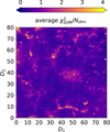 |
Fig. B.1. Similarly to middle panel of Fig. 2, this plot show the SOM grid color-coded according to the average |

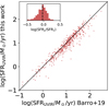 |
Fig. B.2. Comparison between two methods deriving SFR from rest-frame IR, both applied to 509 galaxies at z < 1.8 in the COSMOS-CANDELS area (red dots). The method used in the present work follows Ilbert et al. (2015) and is summarized in Sect. 3.2 (see Eq. 1). The SFRUVIR estimates on the y axis are described in Barro et al. (2019). A solid line shows the 1:1 relationship. The inset in the top-left corner shows a histogram of the difference between Barro et al. (labeled SFRy) and our estimates (SFRx), and a vertical dashed line that marks the median offset at −0.03 dex. |
Another test we made is summarized in Fig. B.3. The goal is to verify the “clustering” of low-mass galaxies in the SOM grid, which alleviate the scatter in the rescaling process of Eq. (3). Even though we did not use individual fluxes as features, the clustering is a consequence of two combined properties: the relationship between colors and M-to-light ratio (e.g., Bell & de Jong 2000, 2001; Zibetti et al. 2009) and the distinctive M-to-light ratios that low-mass galaxies used as comparisons to those at M > 1010 M⊙ (e.g. Bundy et al. 2006; Moffett et al. 2016; Cui et al. 2021).
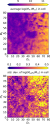 |
Fig. B.3. A more detailed description of how galaxies with different stellar masses are distributed across the SOM. Upper panel: Average log(MLePh/M⊙) of COSMOS2020 galaxies within the same cell, coded according to the color bar above the SOM grid (white cells are empty). Upper panel: Standard deviation of the same log(MLePh/M⊙) distribution per individual cell, coded according to the color bar above the SOM grid (also in this case, empty cells are colored in white). |
All Tables
Optical and NIR data building the observer-frame color space explored by the SOM.
All Figures
|
Fig. 1. Observational properties of the galaxy samples used throughout this work. Upper panel: magnitude-redshift distribution of the COSMOS2020 galaxy sample used to train the SOM (blue color map with hexagonal pixels) after pre-selection at Ks < 24.8 and log(M/M⊙)> 8.5. Individual sources with a 5σ detection in MIPS are overplotted as orange dots. Lower panel: photometric redshift distribution of the COSMOS2020 training set (blue histogram) and the SXDF2018 target sample (green). These data sets are described in Sects. 2.1 and 2.2. |
| In the text | |
|
Fig. 2. SOM of COSMOS2020 galaxies at z < 1.8, selected as described in Sect. 3.1. The same grid is color-coded in three different ways, to show the number of galaxies per cell (left panel), the similarity between galaxies in a given cell and the correspondent SOM weight (middle panel), and the MIPS-detected objects with MLePh > 1010 M⊙ (right panel). In each grid, empty cells are white. Left: handful of cells with only one or two objects are colored in gray. Middle: similarity is quantified by means of Eq. (2). Throughout this work, the dimensions of the 2D grid are arbitrarily labeled D1 and D2 since they have no physical meaning. |
| In the text | |
|
Fig. 3. Illustration of the relationship between input features and the SOM classification (made by the so-called “cells”). This simplified example shows only three broadband colors in the observer’s frame, for a random subsample of 10 000 COSMOS2020 galaxies. |
| In the text | |
|
Fig. 4. Different sets of labels added to the SOM, after training it with COSMOS2020 data. Upper left: redshift labels assigned from the median zLePh of galaxies in the given cell. Upper right: median log(Mlabel/M⊙) per cell, where the Mlabel values are galaxy stellar masses obtained after rescaling every SED to i = 22.5 (Eq. (3)). Lower left: labels from the median SFRlabel per cell applying the same 22.5 mag rescaling as for stellar mass (Eq. (4)); with respect to Fig. 2, a larger portion of the SOM grid is empty because we did not assign a SFRlabel to cells containing only one MIPS galaxy. Lower right: fraction of quiescent galaxies per cell, according to the NUVrK classification (Eq. (5)). |
| In the text | |
|
Fig. 5. Validation of the SOM estimates with “out-of-bag” objects. The COSMOS2020 SOM described in Sect. 3 is built again ten times, excluding every time ∼3000 galaxies randomly extracted from those with a SFRUVIR. The figure compares SFRSOM and SFRUVIR for each SOM realization (histograms of different colors). The Gaussian fit to the ensemble of distributions (green line) has mean μ = −0.005 and standard deviation σ = 0.205 dex. |
| In the text | |
|
Fig. 6. Comparison between stellar masses obtained through standard template fitting (MLePh) and the new method presented in this work (MSOM). The figure shows the density map of 208 404 galaxies in the SXDF field with the magnitude cut at Ks < 24.2. Upper panel: a solid line marks the 1:1 relationship. Bottom panel: the logarithmic ratio log(MSOM/MLePh) is shown as a function of log(MLePh/M⊙), the solid line marks the zero offset while the two dotted lines are set at ±0.3 dex. |
| In the text | |
|
Fig. 7. Quality assessments of the SFRSOM estimates using independent measurements from the literature as “ground truth”. Left panel: comparison between SFRSOM and the template-based estimates from Barro et al. (2019, SFRUVIR) for 608 galaxies at z < 1.8 in the SXDF-CANDELS area (colored dots). For sake of consistency, the Barro et al. (2019) estimates are converted to the same reference system of Ilbert et al. (2015), since the latter has also been used to calibrate the SOM method (see Appendix A). Right panel: comparison to another star formation estimator, that is, Hα nebular emission line. In this case the comparison is performed in COSMOS, for 3718 galaxies (colored dots). In both panels, the color palette from violet to red indicates the stellar mass of each galaxy according to the SOM method; the solid line is the 1:1 relation from which two dashed lines are set at a distance of ±0.3 dex. Each panel also includes an inset that quantifies the dispersion between SFRSOM and the alternate estimate (red histogram); the vertical dotted line marks the median offset, which is −0.05 dex for log(SFRSOM/SFRUVIR) and 0.07 dex for log(SFRSOM/SFRUVIR). |
| In the text | |
|
Fig. 8. Evolution of the main sequence of star forming galaxies resulting from the SOM-based measurement of the SXDF2018 catalog. Redshift bins are chosen to correspond to four time steps separated by ∼2 Gyr, whose color is indicated in the legend along with median redshift and cosmic age. In each bin, the main sequence is identified as the most prominent overdensity in the SFRSOM − MSOM plane (shaded areas representing density contours). Each overdensity peak is fit by Eq. (8) either independently (solid lines) or simultaneously at all t (dashed lines). |
| In the text | |
|
Fig. 9. Redshift evolution of the MS of star forming galaxies (see Sect. 4.3) as determined in the present work (red circles), Ilbert et al. (2015, blue diamonds), Barro et al. (2019, pink squares), Whitaker et al. (2014, blue dotted line), Schreiber et al. (2015, brown solid line), and Leslie et al. (2020, green dashed line). Our estimates stop at the z-dependent threshold for stellar mass completeness defined in Weaver et al. (2022). Their error bars are the 16th–84th percentile range and each symbol is filled with a shade of red according to the completeness of the given mass bin; in particular, dark red symbols represent > 90% completeness, orange between 60 and 80%, while white-filled circles have ≲50% completeness (see Sect. 5.2). Results from the literature are shown only when the median redshift of the given study is sufficiently close to ours (which is indicated in the upper-left corner of each panel); the same measure may be repeated in more than one panel: for example, the MS of Barro et al. (2019) at 0.5 < z < 1 has a median redshift ⟨z⟩=0.8 and it is compared to our data both at 0.6 < z < 0.8 and 0.8 < z < 1.0. |
| In the text | |
|
Fig. 10. Comparison between Barro et al. (2019) and LePhare using the same sample of 608 galaxies also shown in the left panel of Fig. 7. The same BC03 library is fit by LePhare to the full photometric baseline available in the SXDF2018 catalog (filled blue circles) and to the 12 filters only used in the SOM method (open cyan circles). Same colors are used in the inset for the histograms showing the respective log(SFRLePh/SFRUVIR) distributions; the log(SFRSOM/SFRUVIR) distribution (red histogram, same as the inset in the left panel of Fig. 7) is also included as reference. |
| In the text | |
|
Fig. 11. BC03 templates from the LePhare library projected into the SOM. The templates are shifted from z = 0.2 to 1.8 with steps of Δz = 0.01, and perturbed with Gaussian noise to mimic real photometry. The SOM is color coded to show their cell occupation, renormalized to the number density of COSMOS2020 galaxies to make this figure directly comparable with the left-hand panel of Fig. 2. |
| In the text | |
|
Fig. 12. SFR vs. M plane of COSMOS2015 galaxies (colored circles) as it results from the SED fitting performed by the Prospector code (Leja et al. 2021). Only the objects cross-correlated to COSMOS2020 (0.6″ searching radius) are shown, both those having a MIPS 24 μm counterpart (in the upper panel) and objects without FIR detection (lower panel). Each data point is color-coded according to the difference in SFR between Prospector and the SOM estimator. A dashed line at constant sSFR = 10−11 yr−1 is plotted in each panel to guide the eye. |
| In the text | |
|
Fig. 13. Solid lines show the contour density map for the distribution of SXDF2018 galaxies in the SFR–M diagram; this is fit by Eq. (8) as described in Sect. 4.3 (dashed line). Filled circles are SFR median in running bins of galaxies with SFRSOM/MSOM > 10−11 yr−1 (orange symbols) and fQ < 0.5 (red). In both cases, error bars are calculated with the 16th–84th percentile difference. The red circles are interpolated by a linear function (dotted line). |
| In the text | |
|
Fig. 14. Different calibration samples that may be used to label SFR on the SOM. Cells containing galaxies from the original MIPS sample (cf. Fig. 4) are colored in blue; cells containing spectroscopic galaxies with an Hα measurement and radio galaxies with a 3 GHz stacking S/N > 5 are colored in green and red respectively. Colors combine by following the standard RGB rules, e.g. a cell that can be calibrated by both MIPS and Hα (MIPS and radio) is colored in cyan (magenta). A handful of yellow pixels are cells that can be calibrated by only radio stacking and Hα, while white pixels are cells in which all the three star formation tracers are available. As the discussion in the main text is only about coverage and not the actual SFRlabel values, these are not shown in the present figure. |
| In the text | |
|
Fig. 15. Inspection of three SOM cells with coordinates (D1, D2)=[(30, 30),(0, 50),(46, 34)] on the 80 × 80 gird. The first cell (upper panel) has been randomly selected among those with a small galaxy-weight distance Δ (cf. Fig. 2) while the middle and lower panels display two cells located in areas with large Δ values, to provide an insight on SOM shortcomings (see Sect. 5.4). The number of galaxies in these cells is respectively 16, 39, 56. In each panel, the solid line is the median of the BC03 spectral models providing the best fit to each COSMOS2020 galaxy in the LePhare analysis; before calculating the median, all the BC03 spectra (which include only the stellar component, not the nebular emission) have been rescaled to match 22.5 mag in the i band. Such a rescaling also makes easier to compare spectral shapes from the different panels. The gray shaded area encloses the 16th and 84th percentiles of their distribution. The y-axis range in the upper panel is shorter to zoom in the tight 16th–84th dispersion, which would be barely visible otherwise. Filled circles represent the observed photometry, color-coded for the different bands (see legend); for sake of clarity they have been horizontally shifted from the central wavelength of their band by a random offset within ±3%. In the bottom part of each panel we report the average error bars in the same color of their corresponding photometric band. Black crosses are the fluxes that would result from the cell’s weight after training. All symbols are renormalized to the reference i = 22.5 mag. |
| In the text | |
|
Fig. B.1. Similarly to middle panel of Fig. 2, this plot show the SOM grid color-coded according to the average |
| In the text | |
|
Fig. B.2. Comparison between two methods deriving SFR from rest-frame IR, both applied to 509 galaxies at z < 1.8 in the COSMOS-CANDELS area (red dots). The method used in the present work follows Ilbert et al. (2015) and is summarized in Sect. 3.2 (see Eq. 1). The SFRUVIR estimates on the y axis are described in Barro et al. (2019). A solid line shows the 1:1 relationship. The inset in the top-left corner shows a histogram of the difference between Barro et al. (labeled SFRy) and our estimates (SFRx), and a vertical dashed line that marks the median offset at −0.03 dex. |
| In the text | |
|
Fig. B.3. A more detailed description of how galaxies with different stellar masses are distributed across the SOM. Upper panel: Average log(MLePh/M⊙) of COSMOS2020 galaxies within the same cell, coded according to the color bar above the SOM grid (white cells are empty). Upper panel: Standard deviation of the same log(MLePh/M⊙) distribution per individual cell, coded according to the color bar above the SOM grid (also in this case, empty cells are colored in white). |
| In the text | |
Current usage metrics show cumulative count of Article Views (full-text article views including HTML views, PDF and ePub downloads, according to the available data) and Abstracts Views on Vision4Press platform.
Data correspond to usage on the plateform after 2015. The current usage metrics is available 48-96 hours after online publication and is updated daily on week days.
Initial download of the metrics may take a while.