| Issue |
A&A
Volume 664, August 2022
|
|
|---|---|---|
| Article Number | A151 | |
| Number of page(s) | 16 | |
| Section | Interstellar and circumstellar matter | |
| DOI | https://doi.org/10.1051/0004-6361/202243505 | |
| Published online | 24 August 2022 | |
The morphology of CS Cha circumbinary disk suggesting the existence of a Saturn-mass planet
1
Max-Planck-Institut für Astronomie,
Königstuhl 17,
69117,
Heidelberg, Germany
e-mail: This email address is being protected from spambots. You need JavaScript enabled to view it.
2
Departamento de Astronomía, Universidad de Chile,
Camino El Observatorio 1515,
Las Condes, Santiago, Chile
3
Mullard Space Science Laboratory, University College London, Holmbury St Mary,
Dorking, Surrey
RH5 6NT, UK
4
Institut für Astronomie und Astrophysik, Universität Tübingen,
Auf der Morgenstelle 10,
72076,
Germany
5
Unidad Mixta Internacional Franco-Chilena de Astronomía (CNRS UMI 3386), Departamento de Astronomía, Universidad de Chile,
Camino El Observatorio 33,
Las Condes, Santiago, Chile
6
Univ. Grenoble Alpes, CNRS, IPAG,
38000
Grenoble, France
7
Núcleo Milenio de Formación Planetaria (NPF),
Chile
8
Millennium Nucleus on Young Exoplanets and their Moons (YEMS), Universidad de Santiago de Chile,
Av. Libertador Bernardo O’Higgins
3363,
Santiago, Chile
9
Anton Pannekoek Institute for Astronomy, University of Amsterdam,
Science Park 904,
1098XH
Amsterdam, The Netherlands
10
Department of Physics and Astronomy, Rice University,
6100 Main Street, MS-108,
Houston, TX
77005, USA
11
Departamento de Física, Universidad de Santiago de Chile,
Av. Victor Jara
3659,
Santiago
12
Center for Interdisciplinary Research in Astrophysics and Space Exploration (CIRAS), Universidad de Santiago de Chile,
Estación Central,
Chile
13
Instituto de Física y Astronomía, Facultad de Ciencias, Universidad de Valparaiso,
Av. Gran Bretaña 1111,
Playa Ancha, Valparaiso, Chile
Received:
9
March
2022
Accepted:
27
May
2022
Abstract
Context. Planets have been detected in circumbinary orbits in several different systems, despite the additional challenges faced during their formation in such an environment.
Aims. We investigate the possibility of planetary formation in the spectroscopic binary CS Cha by analyzing its circumbinary disk.
Methods. The system was studied with high angular resolution ALMA observations at 0.87 mm. Visibilities modeling and Keplerian fitting are used to constrain the physical properties of CS Cha, and the observations were compared to hydrodynamic simulations.
Results. Our observations are able to resolve the disk cavity in the dust continuum emission and the 12CO J:3–2 transition. We find the dust continuum disk to be azimuthally axisymmetric (less than 9% of intensity variation along the ring) and of low eccentricity (of 0.039 at the peak brightness of the ring).
Conclusions. Under certain conditions, low eccentricities can be achieved in simulated disks without the need of a planet, however, the combination of low eccentricity and axisymmetry is consistent with the presence of a Saturn-like planet orbiting near the edge of the cavity.
Key words: techniques: high angular resolution / planets and satellites: formation / protoplanetary disks / binaries: general
Deceased.
© N. T. Kurtovic 2022
 Open Access article, published by EDP Sciences, under the terms of the Creative Commons Attribution License (https://creativecommons.org/licenses/by/4.0), which permits unrestricted use, distribution, and reproduction in any medium, provided the original work is properly cited.
This article is published in open access under the Subscribe-to-Open model.
This Open access funding provided by Max Planck Society.
1. Introduction
Over the last decade, space telescopes such as Kepler and the Transiting Exoplanet Survey Satellite (TESS) have successfully detected several planets in circumbinary orbits, which are also known as P-type orbit planets (see Doyle et al. 2011; Kostov et al. 2020). These planets have been found to share some orbital properties, such as: (i) most of them are located close to the inner dynamical stability limit (Dvorak 1986; Holman & Wiegert 1999; Martin 2019) and (ii) their orbits are mostly coplanar and of low eccentricity, with a planet occurrence rate similar to single stellar systems (Armstrong et al. 2014; Martin & Triaud 2014). These common characteristics cannot be explained as simply observational biases (Martin & Triaud 2014), which could be evidence that common formation mechanisms are at play for these planets.
Due to the interaction between the two central stars, not all the regions of a circumbinary disk are suitable for planet formation. Tidal forces are expected to carve a central cavity in the disks, where the material density is severely reduced (Artymowicz & Lubow 1994; Miranda & Lai 2015), and oscillations in the eccentricity of the orbits make extremely challenging to have planetesimal and pebble accretion in the regions close or within the dynamical stability limit (Paardekooper et al. 2012; Pierens et al. 2020). Consequently, the detection of several planets in the edge of that region suggests that the planets were formed farther away and later migrated to the location where they can now be observed (Pierens & Nelson 2007; Meschiari 2012; Kley & Haghighipour 2014; Thun & Kley 2018).
Hydrodynamic simulations of circumbinary disks have shown that disks become eccentric due to dynamical instabilities, and the properties of the cavity will be dependent on the binaries and disk itself (see, Lubow 1991; MacFadyen & Milosavljević 2008; Thun et al. 2017; Hirsh et al. 2020; Muñoz & Lithwick 2020; Ragusa et al. 2020). The inclusion of a planet can disrupt this behavior, as the gap opened by a planet can shield the outer disk from the action of the binaries, allowing it to become more circular (Kley et al. 2019; Penzlin et al. 2021). Therefore, the study of a disk kinematics and structures of a young circumbinary disk could either hint at or exclude the presence of such planets.
A particularly interesting multiple stellar system is CS Cha, a spectroscopic binary with a period of at least 7 yr (Guenther et al. 2007; Nguyen et al. 2012) and a member of Chameleon I association, with an estimated age of 4.5 ± 1.5 Myr (Luhman 2007). CS Cha is located at 169 pc estimated from the parallax of Gaia EDR3 (Gaia Collaboration 2016, 2021) and the combined luminosity of the binary is estimated to be L* = 1.45 L⊙ (Manara et al. 2014). The system is known to host a circumbinary disk, which was first identified from its spectral energy distribution (SED) due to an excess in the infrared wavelengths (Gauvin & Strom 1992), and later detected at 1.3 mm wavelength (Henning et al. 1993). The system was cataloged as a transition disk due to its SED shape, which was modeled early on as a disk with a central cavity (Espaillat et al. 2007). Over the last two decades, there have been several attempts to measure the cavity size and ring location, mainly through its SED (Espaillat et al. 2007, 2011; Kim et al. 2009; Ribas et al. 2016), with the latest estimations being  au. Recent observations with the Spectro-Polarimetric High-contrast Exoplanet REsearch (SPHERE) at the Very Large Telescope (VLT) made it possible to spatially resolve the disk scattered light, demonostrating that if there is a cavity in scattered light emission (small micron-sized grains), it must be within the coronagraph hidden region, setting an upper limit of 15.6 au (Ginski et al. 2018). Finally, the modeling of interferometric data of the millimeter dust continuum emission with a 1D radial profile, suggests that the disk has a ring-like shape with its peak located at 204 ± 7 mas (34.5 ± 1.2 au) (Norfolk et al. 2021).
Combined observations of NAOS-CONICA (NACO) at the VLT, SPHERE, and the Hubble Space Telescope (HST), have allowed the identification of a co-moving companion located at ≈1.3″ (≈220 au) of projected distance to the CS Cha binaries (Ginski et al. 2018). Initially, it was thought to be a planetary mass object (Ginski et al. 2018), however, its optical and near-infrared (NIR) spectra have shown that it is possible that CS Cha B is actually an M-dwarf star severely obscured by a highly inclined disk and outflows (Haffert et al. 2020). Such a circumstellar environment on CS Cha B is also supported by a very high degree of polarization observed with SPHERE and by the detection of a mass accretion rate of  M⊙ yr−1 (Haffert et al. 2020).
Motivated by the detection of CS Cha B, the system was observed by Atacama Large Millimeter Array (ALMA) with the aim of characterizing this newly detected companion. These observations also provide one of the deepest and highest sensitivity observations available for a Class II circumbinary disk. In the present work, we analyze the high angular resolution millimeter observations of the CS Cha system, which contains the dust continuum emission at 0.87 mm and 12CO J:3–2 molecular line emission. The observation details and calibration applied to the data are described in Sect. 2. The analysis of the observations and their modeling is presented in Sect. 3, while an attempt to constrain the physical mechanisms responsible of the observed emission structures is detailed in Sect. 4. We discuss our results in Sect. 5, and then we summarize the main conclusions of our work in Sect. 6.
2. Observations
This work includes 0.87 mm observations of the circumbinary system CS Cha, observed with ALMA Band 7 as part of the ALMA project 2017.1.00969.S (PI: M. Benisty) between 26-Nov-2017 and 12-Dec-2017. The correlator was configured to observe four spectral windows: three covered dust continuum emission centered at 334.772 GHz, 336.600 GHz, and 347.471 GHz, with a total bandwidth of 2 GHz; the remaining one was centered at 345.770GHz to observe the molecular line 12CO in the J:3-2 transition (from now on referred to as 12CO) with a frequency resolution of 122.07 kHz (~0.1 km s−1 per channel). The total time on source was 273.1 min, spanning baselines from 15.1 m to 8547.6m from ALMA antenna configurations C43-8 and C43-7.
We started from the pipeline calibrated data, after executing the scriptforPI provided by ALMA. Then, using CASA 5.6.2, we extracted the dust continuum emission from the spectral window targeting 12CO, by flagging the channels located at ±25 km s−1. The remaining channels were combined with the other continuum spectral windows to obtain a “pseudo-continuum” dataset, and we averaged them into 125 MHz channels and 6 s bins to reduce data volume. To enhance the signal to noise ratio (S/N), self-calibration was applied on the continuum. We used a Briggs robust parameter of 0.5 for the imaging of the self-calibration process, and we applied four phase and one amplitude calibrations, using the whole integration time as the solution interval for the amplitude calibration and first phase calibration, while for the remaining phase calibrations, we used 360 s, 150 s, and 60 s.
After self-calibration was complete, we explored different alternative values for the robust parameter to image the data using the CLEAN algorithm. For the multiscale parameter, we used (0*, 0.2*, 0.5*, 1*) the beam size, which, in combination with a smallscalebias of 0.45, returns a smoother model for the emission. This value for smallscalebias is smaller than the default 0.6, which leads to the algorithm preferring the extended scales before point sources. To avoid introducing PSF artifacts that could be mistaken for faint emission, we lowered the gain parameter to 0.05 (it controls the fraction of the flux that is cleaned in every iteration), and increased the cyclefactor to 1.5 (it controls the frequency with which major clean cycles are triggered), both of them chosen for a more conservative imaging compared to the default values1. We cleaned down to a 4σ threshold, and applied the JvM correction to our images, which accounts for the volume ratio ϵ between the point spread function (PSF) of the images and the restored Gaussian of the CLEAN beam, as described in Jorsater & van Moorsel (1995) and Czekala et al. (2021).
The calibration tables obtained from the dust continuum self-calibration were applied to the molecular line emission channels, and then the continuum emission was subtracted from them with the uvcontsub task. To increase the S/N of the images, we imaged the 12CO channels with a lowered velocity resolution of 0.25 km s−1, centered at 3.65 km s−1, which is approximately the velocity at the local standard of rest (VLSR). Different robust parameters ranging from −1.2 to 1.2 were explored to find the best trade-off between angular resolution and sensitivity. Additionally, we also applied uv tapering2 to generate another set of 12CO images with a more circularized beam.
The JvM correction was also applied to the CO channel maps before any analysis was carried out on them. The package bettermoments (Teague & Foreman-Mackey 2018; Teague 2019b) was used to create additional image products from the channel maps. This package fits a quadratic function to find the peak intensity of the line emission in each pixel, and the velocity associated with it, but we also used it to generate the moment 0 and moment 1 of each velocity cube. All the moment images were clipped at 3 sigma and no mask was used.
To accurately analyze the observations, we also applied uv modeling to the continuum visibilities of the source, as described in Sect. 3.3. To further reduce the data volume after finishing the self-calibration, we averaged the continuum emission into 1 channel per spectral window (as in Andrews et al. 2021) and 30 s of time binning. We used each binned channel central frequency to convert the visibility coordinates into wavelength units.
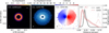 |
Fig. 1 Reconstructed images of dust continuum emission and 12CO. From left to right: dust continuum emission from CS Cha imaged with a robust parameter of −0.5, moment 0 and moment 1 of the 12CO imaged with a robust of −0.2, and radial profiles for the continuum and 12CO emission calculated by deprojecting the images with the inclination and position angle of Model 2e (see Sect. 3.3). The ellipse in the left bottom corner of the panels represents the synthesized beam of the images, which is 30 * 46 mas for the dust continuum and 80 * 77 mas for the 12CO. The scale bar in the top right of the first panel represents 20 au at the distance of the source. The Gaussians in the right panel represent the average radial resolution of the profiles, and in the same panel, the colored region in the profiles represent the 1 σ dispersion at each radial location. |
3. Observational results
3.1. Circumbinary disk: Dust continuum emission physical properties
The millimeter emission is resolved into a single disk around the binary stars (a circumbinary disk), as shown in Fig. 1 after being imaged with a robust parameter of −0.5, returning an angular resolution of 30 × 46 mas. At a nominal resolution (61 × 87 mas with a robust parameter of 0.5), the disk appears as a single smooth ring with a central cavity, however, higher angular resolution images resolve the disk radial structure, showing evidence of a radially asymmetric ring (right panel of Fig. 1). A gallery with the dust continuum emission reconstructed with different robust parameters ranging from −1 to 1 is included in Fig. A.1 in the appendix. For continuum images with robust parameters larger than 1, the sensitivity changes are negligible, as the beam size increases to an extent less than 10% and the point spread function is poorer due to the sparser uv coverage at short baselines compared to long baselines, resulting in stronger sidelobes and, thus, stronger structured residuals.
The radial profiles were obtained by deprojecting the images with the geometry parameters obtained in Sect. 3.3 (inc = 17.86 deg and PA = 82.6 deg, see Table 1), where we considered multiple Gaussian components and eccentricities to describe the circumbinary disk. We find that the dust continuum ring profile peaks at 205 ± 5 mas from the disk center, which is 34.6 ± 0.8 au at the distance of the source. Since it was calculated from the image, we used 5 mas as a conservative uncertainty (the pixel size), which is consistent with the previous study by Norfolk et al. (2021).
In order to estimate the optical depth τ of the emission, we followed the same approach as in Pinilla et al. (2021), assuming that the disk emits as a black body and therefore τ = − ln(l − TB/Tphys), where TB is the brightness temperature, and Tphys is the physical temperature of the midplane. We estimated the TB from the different dust continuum images by starting from the Rayleigh-Jeans approximation. When the beam size is increased (by using larger robust parameters), the emission becomes more diluted and, so, the peak temperatures decreases. For the image with a robust parameter of 0.5, the peak brightness temperature of the image reaches 12.3 ± 0.1 K (brightness temperature uncertainty given with 3 sigma confidence), while for the image with robust value of −1.0, it reaches 17.4 ± 0.4 K, since the ring is better resolved. For this reason, we decided to use the image generated with robust −0.5 to estimate the optical depth, given it has a high S/N and also high spatial resolution. From this image, we obtained a peak TB of 16.1 ± 0.3 K.
For the Tphys, we need additional assumptions. If we consider the midplane temperature to be at the standard 20 K, then we find a peak optical depth of τpeak = 1.34. On the other hand, if we consider the approximated luminosity-dependent temperature relation from Andrews et al. (2013), T = 25(L*/L⊙)0.25 K, and L* = 1.45 L⊙ for the stellar luminosity (Manara et al. 2014), then we can estimate Tphys = 27.4 K and τpeak = 0.77. Both estimates should be considered with caution, as the first assumes a single constant temperature and the latter comes from a luminosity relation for disks with a single stellar host.
We calculated the dust mass of the model by assuming that the flux (Fv) received has a wavelength of 0.87 mm and is being emitted by optically thin dust with a constant temperature of 20 K (as in Ansdell et al. 2016; Pinilla et al. 2018), and, alternatively, with a constant temperature of 27.4 K. In both approaches, we follow Hildebrand (1983):
 (1)
(1)
where d is the distance to the source, v is the observed frequency, Bv is the Planck function at the frequency v, and kv = 2.3(v/230 GHz)0.4cm2 g−1 is the frequency-dependent mass absorption coefficient (as in Andrews et al. 2013). The total flux from the source is estimated by taking the weighted average of the baselines shorter than 28 kλ, which gives Fv = 180.2 ± 0.5 mJy, not accounting for the 10% uncertainty of ALMA fluxes. We chose to measure it from the visibilities that do not resolve the disk emission to avoid introducing additional uncertainties related to image reconstruction and possible dependence on the mask chosen. Replacing this value in Eq. (1), we obtain a dust mass of 69.0 ± 0.1 M⊕ when assuming Tphys = 20 K, and 44.7 ± 0.1 M⊕ for Tphys = 27.4 K. Therefore, the dust mass content is uncertain either because of the temperature assumption and the poor constraints that we have on the dust opacities from the observations.
Best parameters from the uv modeling.
3.2. No detection of emission near CS Cha B
We did not detect any significant emitting source at the expected location of CS ChaB, neither in dust continuum emission nor 12CO, as shown in the upper and lower panels of Fig. 2, respectively, where the emission has been saturated to 5σ of each image. In the dust continuum, by using our highest sensitivity image (generated with a robust parameter of 1.0) and based on the assumption that CS Cha B is a point source, we can estimate a 3σ upper limit for millimeter emission to be 35.4 μJy. This emission translates into a dust mass upper limit of MB < 0.015 M⊕ under the assumption of 20 K and optically thin emission. Even if the disk is not a compact source, the beam size of the robust 1.0 image is ~18 × 13 au at the distance of the source, therefore, the dust disk would have been unresolved even if it had a size of 10 au.
In 12CO, we do not detect any significant emission at the location of CS ChaB either and this non-detection is independent from the channel map velocity width and synthesized beam size used for image reconstruction. As a final test for the detection of CS Cha B, we generated a cube with a robust parameter of 1.2, no uv tapering, and a channel width of 1 km s−1 , going from −24 to 24 km s−1 around the rest frame of the 12CO line. These channels were all stacked and the result is displayed in the lower panel of Fig. 2. The peak emission within the square mask does not reach a significance of 2σ.
3.3. Dust morphology from the visibility fitting
To precisely constrain the structure of the dust continuum emission, we applied uv modeling to the visibilities of the source, via parametric models. In principle, the brightness profile (f) of an axisymmetric disk would only depended on the radial distance to the center of the disk (given by f := f (r)). However, circumbinary disks are expected to display some eccentricity due to the interaction between the disk material and the binaries (e.g., Thun et al. 2017; Kley et al. 2019), and so, it is convenient to define the brightness profile not as a function of the radius, but as a function of the semi-major axis instead (f := f(a)). We calculated the eccentric coordinate system by following the same approach that Marino et al. (2019) and Booth et al. (2021):
 (2)
(2)
where the semi-major axis α is a function of the radial distance from the center of mass and the azimuthal angle (r, ϕ), and it can also be modified by the eccentricity, e, and the argument of the periastron ω. It is pertinent to notice that this coordinate system does allow for the solution e = 0.0, which returns the standard polar coordinates.
Several models with increasing complexity have been considered to describe the disk around CS Cha, which are composed of a combination of Gaussians shapes by f = ∑igi, where gi is the ith Gaussian. Each subsequent model is motivated by the residuals of the best previous model, but they all share the same basic shape for the disk, described by a bright Gaussian ring (g0) for the inner side of the ring emission, plus a radially asymmetric Gaussian ring (g1) to describe the outer side of the ring emission. This g1 component has a different width for each side of its peak, also known as broken-Gaussian ((σi, σo) for the inner and outer part, respectively). The additional features considered in the more complex models were a centrally peaked Gaussian (g2) and an extended Gaussian ring (g3). All these components are schematized in Fig. A.3, and the ones considered in each model are: (i) Model 2g, composed of g0+gi with eccentricity and argument of the periastron of (e0,ω0); (ii) Model 3g, composed of g0+g1 +g2 with (e0,ω0); (iii) Model 4g, composed of g0+g1 +g2 +g3 with (e0,ω0); and (iv) Model 2e, composed of g0+g2 with (e0,ω0), and g1+g3 with (e1,ω1);.
The CS Cha disk is close to being face-on (as seen in Fig. 1) and so, the dust continuum modeling has a strong dependence between the center of the disk (x0, y0), the inclination (inc), the position angle (PA), and the eccentricity parameters (e, ω). To reduce the number of free parameters, we used the 12CO observations (which are independent from the dust continuum observations) to constrain the PA of the disk. As explained in Sect. 3.4, the preliminary kinematic fittings to the 12CO show that it has a position angle of 82.6 deg, and so we fix this value in our uv modeling.
To find the best set of parameters for each different model, we used the package emcee to sample the parameter space with a Markov chain Monte Carlo (MCMC) Ensemble Sampler (Foreman-Mackey et al. 2013), using 250 walkers and a flat prior for all the parameters. We used galario to compute the visibilities of the synthetic images, which were generated with a pixel size of 5 mas, as the images from tclean. The total flux of the model is calculated by averaging the real part of the ten shortest baselines (u-v pairs) after convergence, and we picked 5000 MCMC random walkers positions to calculate the uncertainty of the flux.
The best parameters for each model and their uncertainties are summarized in Table 1. All the models show consistent results for the disk flux (Fλ), the location of the radius that includes the 68% and 90% of the flux (R68 and R90), and the location of the peak of the ring (given by the parameter r0). The difference between the models can be better observed when the residuals are imaged, as seen in Fig. 3 for the Model 2e, and in the Fig. A.4 for the Models 2g, 3g, and 4g. The simplest model, Model 2g, shows strong structured residuals in the ring region, and also in the cavity, evidence that the cavity is not completely depleted of dust continuum emission. Then, Model 3g takes into account this inner cavity emission with a Gaussian that peaks at the center of the disk (g2), however, this Gaussian is spread over the whole disk in the attempt to account for an extended diffuse emission, rather than only fitting the cavity emission. To fix this behavior, Model 4g includes a new diffuse extended Gaussian for the ring (g3) in addition to the Gaussian for the inner cavity emission (g2). It ultimately succeeds at describing the cavity emission, but still leaves structured residuals in the circumbinary ring.
The residuals from the Model 4g subtracted too much flux from some regions (seen in blue in the residual image), and not enough from others (seen in red in the residual image). The structure of these residuals cannot be explained by any combination of offsets in center (δRA, δDec), nor geometry (inc, PA), which is discussed in depth in the Appendix of Andrews et al. (2021). To account for the residuals of Model 4g, two additional models were considered: (i) a model where the innermost emission has a different inclination compared to the outer most regions (g0+g2 have a inclination inc0, while g1+g3 have another inc1), but they share the same eccentricity; and (ii) a model where those components have the same inclination, but different eccentricities. The model with different inclinations returned residuals that were similar to the ones from Model 4g, and the inclinations (inc0, inc1) were not disparate from the noise level. On the other hand, the model with two eccentricities (Model 2e) was successful in accounting for the structured residuals observed in the circumbinary ring, as seen in Fig. 3.
The best model, Model 2e, found two different eccentricities for the inner most emission and the outermost emission from the circumbinary disk, with the inner ring eccentricity (e0 = 0.39) being about twice that of the outer disk eccentricity (e1 = 0.19), as shown in Table 1. We calculated the mass of the dust in the model by following the same assumptions we took in the dust continuum images: optically thin emission and 0.87 mm, with dust at 20 K. The flux from all components of Model 2e adds up to 180.57 ± 0.05 mJy, which translates into a dust mass of 69.05 ± 0.02 M⊙ at the distance of this source (not considering the 10% uncertainty of ALMA fluxes). As for central Gaussian, g2, alone in the Model 2e, we find a flux of 150 ± 16 µJy, or a dust mass of 0.057 ± 0.006 M⊙ being detected inside the cavity. This dust mass is ≈0.5 MMars, or ≈5 MMoon, for reference.
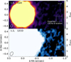 |
Fig. 2 High-sensitivity millimeter emission images of CS Cha. Upper panel: dust continuum image generated with a robust parameter of 1.0. The color scale is linear and has been saturated to show the emission between 0 and 5σcont, with σcont = 11.8 μJy beam−1 being the rms of this image. A box of 0.2″ per side is centered at the expected location of CS ChaB. The beam size is 105 × 75 mas, and is shown in the lower left corner of the figure. The scale bar at the top right represents 20 au. Lower panel: 12CO emission image generated with a robust parameter of 1.2, after stacking all the channel maps between −24 and 24 kms−1 around the rest frame. The beam size is 148 × 97 mas, and is shown in the lower left corner of the figure. The color scale is linear and has been saturated to show the emission between 0 and 5σ12CO, with σ12CO = 1.4 mJy beam−1 being the rms of this image. |
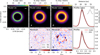 |
Fig. 3 Best solution for the dust continuum emission generated using the Model 2e, which considers two eccentricities for the disk components. Upper row: left panel shows the synthetic image of the best model found. Middle panels show how this model would have been observed by ALMA with two different robust parameters, comparable to the images from Fig. A.l. Right panel shows the radial profile obtained from the beam convolved images generated with a robust parameter of 0.0, and the average beam resolution shown with a Gaussian in gray. Lower row: middle panels show the residuals left by the best model, imaged with two different robust parameters shown in the upper left corner. Right panel shows the intensity profile of the model obtained from tclean and the best Model 2e (not convolved by beam). |
3.4. 12CO J:3–2 emission
3.4.1. Emission profile of the 12CO emission
We generated images for the 12CO emission from CS Cha with different robust parameters to check the emission at a high angular resolution, but also to check the extended structure with high S/N. The channel maps were all generated with the same velocity channels, and their only difference is the robust parameter used. A gallery of the channels generated with robust 0.0 is shown in the appendix (Fig. A.2).
The 12CO emission (shown in Figs. 1 and 4) appears depleted in the central region of the cavity, and the brightness peak is located at 128 mas (or 21.6 au), which is closer to the center of the disk compared to the dust continuum radial profile, which peaks at 34.6 au. The profile recovered from the different moment 0 images consistently show the brightness peak at the same radial location. By using the inclination from the continuum fit, plus the vertical structure and PA traced by a kinematic fit with the eddy package (Teague 2019a) (as described in the following Sect. 3.4.2, and summarized in Table 2), we deprojected the 12CO Moment 0 image and used it to calculate an azimuthally averaged surface brightness profile (shown in Fig. 4).
We subtracted the azimuthally averaged surface profile from the 12CO moment 0, to search for asymmetries. The moment 0 is preferred over the peak intensity map as the latter is more affected by the beam size and geometry of the disk, thus creating overbrightness regions along the major axis which are not of physical origin. When an azimuthally symmetric model is subtracted from the moment 0, the disk shows residuals on extended and compact scales, with a typical contrast between the emission and model on the order of <15%. The brightness temperature of the 12CO moment 0 reaches about 120 K at the radial profile peak and decreases towards about 10 K in the outer edge. Due to this temperature range, the emission is possibly more optically thick in some regions than in others and, thus, its brightness traces a combination of temperature and gas density variations at the disk surface layers. These residuals may originate from a combination of small-scale height variations, disk eccentricity and dynamical perturbations, and none are included in the azimuthally averaged surface profile.
Best parameters from the kinematic fitting with eddy to the image generated with a robust parameter of 0.0.
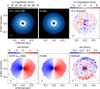 |
Fig. 4 CS Cha gas emission and kinematics. Upper row: 12CO moment 0, the best model using the geometry recovered from the kinematic fit, and the residuals. Scale bar represents 20 au at the distance of the source. Lower row: 12CO peak velocity in the line of sight, with the best model calculated with the parameters from Table 2, and the residuals. The dashed line shows the mask used for the fit. |
3.4.2. Kinematics of the 12CO emission
We calculated the velocity map of the 12CO by using the package bettermoments, which fits a quadratic function to each pixel over the channel maps cube, allowing us to obtain the velocity corresponding to the peak emission with sub-channel velocity resolution. The velocity map used in the kinematic analysis is shown in Figs. 1 and 4. Additionally, a careful analysis of the channel maps in Fig. A.2 allows us to confirm that the southern side of the disk is closer towards us, and so the disk is rotating counter-clockwise from the observers’ point of view. This coincides with the projected direction of the proposed orbits for CS Cha B (Ginski et al. 2018), however, its orbital plane has not been accurately constrained and it might not necessarily be coplanar to CS Cha.
As discussed in the Sect. 3.3, with the disk being so close to face-on, there are correlations that are difficult to disentangle without fixing some geometric parameters. In the case of the12 CO kinematic image, there is a strong correlation between the total mass of the central stars Mtotal, the inclination of the disk (inc), and the surface layer geometry from where the 12CO is being detected, which we describe as a function of the radius from the center of the disk (hco (r)). Due to the low inclination of the disk, a variable that is mostly independent from the previous unknown parameters is the PA of the disk, and so it is the first value that we constrain.
We used the eddy package to fit the 12CO kinematic map under the assumption of flat disk, to avoid introducing additional free parameters while the inclination and Mtotal are still not constrained. We run a MCMC with uniform prior over the six free parameters that include the center of the disk (x0, y0), the disk geometry (inc, PA), the binaries mass (Mtotal), and velocity at the local standard of reference (VLSR), and we recovered a value of PA = 262.6 ± 0.1 deg, which is consistent for kinematic maps generated from different robust parameters. This value is higher than 180 deg since the convention used in this kinematic fitting is that the PA is aligned with the red-shifted part of the disk. If we follow the dust continuum emission convention of measuring the PA as the angle between the north and the semi-major axis to the east, we obtain PA = 82.6 deg (this includes an assumption of a flat dust continuum disk). This value is used in the uv modeling of the dust continuum (shown in Sect. 3.3), from where we find an inclination of the midplane of inc= 17.86 deg, which we assume to be the inclination for the 12CO emission.
By having the inclination fixed, the degeneracy of the value for Mtotal is reduced, enabling us to include as free parameters the description for the vertical height (zCO(r) of the emitting surface layer. We perform this new fit under the assumption of a single power law, following zCO = z0 · rψ, where the free parameters are the pair (z0, ψ), and it is only a function of the distance to the disk center r. The Keplerian velocity is calculated by including the scale of the height 12CO in the distance to the center of the disk, based on the following:
 (3)
(3)
The best parameters obtained after running a MCMC optimizer with the new model are listed in Table 2, where we recover the central mass of the stars: Mtotal ≈ 1.91 M⊙. The kinematic image of the best model, and the residuals, are shown in the bottom-middle and bottom-right panels of Fig. 4, respectively, where the mask used to fit the velocity map is shown: an annulus with inner radius of 0.15″ and outer radius of 0.65″. Given that our model does not includes eccentricity, the inclusion or exclusion of different regions of the disk can change the position of the centroid, which, in turn, also affects the best fit parameters. Depending on the masked region used to fit the velocity map, the mass of the central object can shift between 1.86−1.91 M⊙, due to changes in the position of the center. The non-eccentric kinematic model is also the reason for which the values of δRA and (δDec do not match between the dust continuum and 12CO fits.
In principle, the eccentricity is expected to decrease for regions that are located farther away from the binaries. Fitting those regions with a kinematic model should therefore lead to a better determination of the disk barycenter position. In CS Cha, however, there are two issues with including the outer-regions in the velocity fit: (i) the S/N is decreased towards the outer edge of the disk, thus not allowing us to distinguish between the emission from the front-side and back-side of the disk; and (ii) the line following the zeroth velocity at different radius (in our line of sight), known as the line of nodes, is curved in the outer regions of the disk (as can be better seen in the left panel of Fig. 4 and channel map 3.65 in Fig. A.2). The mechanisms driving the velocity residuals inside and outside of the mask are still a subject to be studied. In the disk cavity, the residuals could be a combination of eccentric gas flow due to the binaries, and also radial flows of material flowing from the main ring towards the binaries, as described in Rosenfeld et al. (2014). As for the outer disk, the residual velocities could show a combination of eccentricity (which is not accounted in a circular model), and tidal influence from the companion CS Cha B. Such tidal interaction has been observed in other disks in multiple-stellar systems, such as AS 205 and RWAur (Kurtovic et al. 2018; Rodriguez et al. 2018, respectively).
4. Hydrodynamical simulations
We compared our ALMA observations with hydrodynamical simulations of circumbinary disks, to test the general conditions that could generate the observable characteristics of CS Cha. Our main focus was the comparison between the cavity and ring properties in circumbinary disks that do and those that do not host a single Saturn-like planet, as we describe in the following subsections.
4.1. Setup: Circumbinary disk with FARGO3D
We ran our simulations in a modified version of the FARGO3D code (Benítez-Llambay & Masset 2016) used in Thun & Kley (2018) to simulate a 2D-hydrodynamical model of a circumbinary disk with the stellar properties of CS Cha. As in Thun & Kley (2018) and Penzlin et al. (2021), we simulated the disk with a cylindrical grid, starting at an inner radius of 1 abin up to 40 abin (with abin the binary separation), with 684 logarithmically spaced radial cells and 1168 azimuthal cells, which is twice the azimuthal resolution used in the previously mentioned works. This higher resolution is applied to ensure convergence when the planet is included, and the results with half resolution are consistent with the ones shown in the following sections. The total binary mass was obtained from our eddy fit (Mtotal = 1.91 M⊙), and the mass ratio used for the binaries is q = 0.7, calculated in Ginski et al. (in prep.) by using the R-band and I-band magnitudes of SPHERE ZIMPOL observations (Beuzit et al. 2019; Schmid et al. 2018).
For the surface density, we used a radially dependent profile given by Σ(r) = fgap · Σ0 · r−3/2, where r is the radial distance from the disk center, Σ0 is chosen such that the disk mass is 0.01 Mtotal, and fgap is an exponential function that depletes the density profile inside 2.5 abin, therefore speeding up the number of orbits needed to reach the steady state. We calculate fgap as in Thun et al. (2017), by using fgap = (1 + exp [− (r − 2.5 abin)/(0.25 abin)])−1. All our simulations have fixed α viscosity parameter of α = 10−4 (Shakura & Sunyaev 1973) for all radii.
Our simulations use a locally isothermal equation of state for the gas, which allows for a faster convergence compared to a viscous heated radiative disk. In the latter, the steady state of the gas is comparable to the isothermal setup for a constant disk aspect ratio h/r, but it can take over 100 000 orbits to be reached (Kley et al. 2019). We set our binaries such that they are only sensitive to each other (and not to the disk around them).
Due to the long period of their orbit (at least 2482 days, Guenther et al. 2007), the separation of the components and their eccentricity is only constrained to be within a certain parameter range (abin < 7.5 au and ebin ≲ 0.5, Ginski et al., in prep.). Given that the simulations can be run with normalized units, the uncertainty in the binary separation can be circumvented by treating distances in terms of the binary separation, but to account for the possible binary eccentricities, we need to run simulations with different values. Therefore, we ran three different binary eccentricities setups: ebin = [0.15, 0.25, 0.35], and we let them evolve for 20 000 binary orbits to reach the steady state. As the circumbinary disks have minimal eccentricity for ebin ≈ 0.15, we sampled the allowed eccentricity range for ebin with increasing eccentricities starting from the smallest (Thun & Kley 2018; Kley et al. 2019). Additionally, previous works have shown that different aspect ratios can have an impact in the disk gas morphology (Thun & Kley 2018; Tiede et al. 2020; Penzlin et al. 2021); therefore, we ran each binary eccentricity with 2 aspect ratios: h/r = 0.03 and h/r = 0.05.
After 20 000 orbits, we introduced a single planet at a distance of 6 abin and we let it migrate inward to its equilibrium orbit. From Kley et al. (2019), we know that the planet ability to open a gap determines its evolution. Planets that are able to open a gap can separate the outer disk from the inner disk, effectively shielding the outer disk from the binaries action, lowering the eccentricity of these regions. Since we are running simulations in a low viscosity scenario, we decided to use a giant planet of low mass Mp = 1 MSaturn, which is consistent with the planets detected in P-type orbits (Penzlin et al. 2021).
Previous studies have also found that more massive planets, such as 1MJup, are prone to more unstable orbits and have a higher likelihood of getting excited into a larger distance orbit or even of getting ejected from the system (Pierens & Nelson 2008).
After introducing the planet, we ran each simulation for another 100000 binary orbits, which is 50000 orbits after the convergence of five out of six of our migrating planets. For comparison, we also kept running the simulations without a planet for 100000 additional binary orbits. This leaves us with 12 simulations when taking into account all binary eccentricities, disk aspect ratios, and planet presence. A summary of the setups is found in Table 3.
Eccentricity and semi-major axis of the cavity edge (ecav, acav), peak density (epeak, apeak), and planetary orbit (epl, apl).
4.2. Disk evolution with no planet
In the absence of a planet, the disk cavity quickly becomes eccentric, with the size of the cavity and its precession velocity being dependent on the eccentricity of the binaries (ebin) and the disk aspect ratio (h/r). In order to measure the cavity properties, we trace the cavity boundary by searching for the radial position at which the density reaches 10% of the peak density, and we repeat for every azimuthal element of the gas density image, thus obtaining 1168 radial positions for each time step. This 10% threshold is chosen to avoid the streamers of material that flow from the circumbinary ring onto the binaries. We fit these points with an eccentric orbit by using the function curve_fit from the Python package scipy.optimize (Virtanen et al. 2020). The best fit allows us to recover the eccentricity of the cavity (ecav), the semi-major axis (acav), and the argument of the periastron (ωcav), which is used to trace the cavity precession.
We show the cavity boundary fit for the binary orbit 100 000 with a white dashed line in Fig. 5, and the median value of acav and ecav the last 1000 binary orbits is shown in Table 3. Alternatively, another approach to recover the eccentricity information of the disk is through the eccentricity vector, which uses the kinematic information and returns the eccentricity of a gas parcel. We find consistent results between both methods (calculating from density compared to eccentricity vector), and we decided to go with the density-based estimation to be consistent with our uv modeling approach to recover eccentricity.
As expected, the smallest ecav and acav are obtained for the binaries with eccentricity of 0.15, which at the end of the simulation have a semi-major axis acav < 4 abin in both aspect ratio setups. The biggest cavity sizes of all setups are found for the binaries with eccentricity of 0.35, with a final cavity size acav > 4.5 abin. Overall, the difference between smallest and biggest cavities is only about 15%. We also find that neither ecav nor acav are constant in time, as they have an oscillatory behavior with shorter period for smaller binary eccentricity, shown in Fig. 6. A quick analysis with a periodogram allowed us to find that the oscillations period in ecav and acav are almost identical to the precession period of ωcav, which ranges between 1100 to 2300 Tbin depending on the binary eccentricity and disk aspect ratio. Considering a binary period of 7 yr for CS Cha, a complete precession of the cavity would be observable over a period of at least 7700 yr, considering the shortest precession period of our simulations.
We also traced the radial positions at which the gas density is highest for each azimuthal element (a peak gas density ring), and we fit an eccentric orbit in the same way it was done for the cavity, allowing the recovery of the eccentricity epeak, semi-major axis apeak, and argument of the periastron ωpeak. The best fit to the peak positions is shown in Fig. 5 with black dashed lines for the binary orbit 100 000, and the median values for the last 1000 binary orbits for all setups is shown in Table 3. In the absence of a planet the values for epeak can go from 0.03 to almost 0.1, while apeak ranges between 4.6 and 6.2 abin. Similar to the cavity, the peak density ring also shows an oscillatory behavior on its parameters, which is shown in Fig. 7 for the last 15 000 orbits (in reddish colors).
Another significant feature that can be drawn from the simulations is the azimuthal density variation along the density peaks, which can be better appreciated in Fig. 5. Due to the eccentricity of the disks, there is an over-density at the location of the apoastron of the orbits, which is a product of the slower orbital velocities at that location compared to the periastron orbital velocity. We measure the contrast between the highest density and lower density along the peak density ring by calculating qpeak = ρmax/ρmin, where ρ is the gas density. This value is reported in Table 3, and we find that the binaries with 0.15 of eccentricity have the least asymmetric rings for the no planet setups, with an excess of at least 40% between maximum and minimum density.
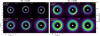 |
Fig. 5 Gas surface density after 100 000 binary orbits in each setup. Distance is in binary separations and the color scale is normalized to the maximum of each image. Panels on the left and right show the setups with h/r = 0.03 and h/r = 0.05 respectively. In each panel, the columns show the setups with the same binary eccentricity, being 0.15, 0.25, and 0.35 from left to right. The upper row of each panel contains the setups with no planet, and the lower row the setups with planet. A white dashed line shows the best cavity fit, while the black dashed line shows the best peak ring fit. A white triangle is used to show the position of the planet. |
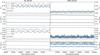 |
Fig. 6 Eccentricity and semi-major axis for the cavity (ecav, acav) as a function of time in binary orbits. Each panel contains the simulations of the three different ebin for the binaries, and a single aspect ratio, displayed in the left-side together with the line-style legend. |
4.3. Disk evolution with a Saturn-like planet
The planet starts migrating inwards and carving a gap as soon as it is introduced into the simulation. The evolution of the planet’s eccentricity and semi-major axis is shown in Fig. 8. Depending on the binary eccentricity, the planet takes different times to converge to its steady orbit, and the longest time for convergence is obtained for the planet around binaries of eccentricity ebin = 0.15. After 50000 binary orbits, the planet in most of the simulations has converged to its steady semi-major axis (apl), which ranges between 3.3 to 4.0 abin, depending on the binary eccentricity and disk aspect ratio. The only planet that takes more than 50 000 binary orbits to converge to its final position is the planet in the setup ebin = 0.35 with h/r = 0.03, as shown in the left panel of Fig. 8. As the eccentricity of the binaries is increased, the instability region is pushed farther away, thus the initial position of this planet was more unstable than the others.
The planet is initially pushed to a farther orbit, before it starts migrating inwards as the others. Examples of this behavior are also seen in Penzlin et al. (2021), where some of the planets would even get ejected from the system depending on the binary mass ratio, eccentricity and disk aspect ratio, for the same initial planet position. As this planet jumps into a higher orbit, it creates a secondary ring outside the main ring excited by the binaries, with a gap between them located roughly at 8 abin. After the planet has migrated inwards into the cavity, the secondary ring remains as a stable structure until the end of our simulations.
The eccentricity of the planet orbit epl is not constant with time, and it oscillates between 0 and 0.05 in both aspect ratio setups (as shown in the lower panel of Fig. 8). By analyzing the periodogram of epl (after apl convergence), we find the oscillation period to be consistent with the cavity oscillations periods, in agreement with the findings of Penzlin et al. (2019), where multiple planets were considered.
The planets modify the structure of the cavity and the overall disk eccentricity. To quantify the difference between the setups with and without planets, we calculated the cavity properties and peak density ring properties following the same procedures explained in Sect. 4.2. The planet presence considerably decreases ecav, as shown in Fig. 6, where the highest amplitude variations do not reach the minimum ecav from the no planet setups, independently from the ebin and disk aspect ratio. This oscillations are consistently confined to the range between (0.0, 0.1) for the aspect ratio h/r = 0.05, and (0.0, 0.03) for the aspect ratio h/r = 0.03. As in the “no-planet” simulations, the period of the oscillations in ecav and acav are consistent with the cavity precession period, and they coincide with the oscillation period of epl.
The decrease in eccentricity due to the planet’s presence is extended towards the whole disk. The only case where peak ring eccentricities become comparable between setups with or without a planet is for the aspect ratio h/r = 0.05, where the setups without planet and ebin = 0.15 and 0.25 have epeak in the same eccentricity range of with planet setups (as shown bottom panel-pair in Fig. 7). The overall decrease in eccentricity contributes to a decrease in the density asymmetry along the peak density ring, as the gas spends similar amount of time in each azimuthal element. Considering all our simulations, we find the gas density profile to be between three to seven times more axisymmetric when the planet is present, as shown in Table 3.
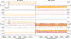 |
Fig. 7 Eccentricity and semi-major axis for the peak density ring (epeak, apeak) as a function of time in binary orbits. Each panel contains the simulations of the three different ebin values for the binaries and a single aspect ratio, displayed in the left-side together with the line-style legend. |
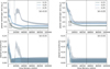 |
Fig. 8 Planet’s semi-major axis and eccentricity as a function of time (in binary orbits) in the upper and lower panel row, respectively. The upper right number in each plot indicates the eccentricity of the binaries. The dashed vertical curve indicates the position of the 50 000 binary orbits, after which the planet has converged to its equilibrium orbit. The median semi-major axis for the planet orbit after convergence is indicated with a dotted line. |
5. Discussion
5.1. Non-detetion of CS Cha B
Despite the strong evidence of a highly inclined disk around CS Cha B (high polarization fraction, optical and NIR attenuation, and accretion rate Ginski et al. 2018; Haffert et al. 2020), our observations are unable to detect such material at 0.87 mm wavelength. For comparison, the 35.4μm limit is three times fainter than the detected flux from PDS70c (Benisty et al. 2021) or the free floating planet OTS 44 (Bayo et al. 2017) – and it is even lower than the upper limits found for protolunar disk fluxes of directly imaged exoplanets (Pérez et al. 2019).
The non-detection of CO towards CS Cha B suggests that its emission is either being blocked, or that its CO emitting layer is very compact (or a combination of both). Disks around M-dwarf stars are expected to be smaller compared to disks around Sun-like stars (Andrews et al. 2013; Tripathi et al. 2017; Hendler et al. 2020), and the tidal interaction of CS ChaB with the main CS Cha system could have further truncated its size (Bate 2018; Cuello et al. 2019; Manara et al. 2019). Observations at shorter wavelengths (such as ALMA bands 8-10 or JWST instruments MIRI and NIRcam) are needed to fully understand the circumstellar environment of CS Cha B, by connecting the non-detection in 0.87 mm to the NIR observations.
Alternatively, CS Cha B could also be a young source located in the background of the Cha I cloud. In such scenario, a diskless star (or a very small disk) would explain the non-detection at mm wavelengths, while the light would be additionally obscured and polarized by the environment. The Ha emission could be a contribution from accretion and chromospheric activity (e.g. PZ Tel B, Musso Barcucci et al. 2019), and the apparently common proper motion would be due to both systems being on the same cloud. A longer time baseline on the sources astrometry could clarify whether the sources are indeed gravitationally bounded or whether their apparent proximity and similar proper motion is only a temporary coincidence.
5.2. A Saturn-like planet is consistent with the morphology of the CS Cha disk
Two main properties distinguish the simulated disks that host a Saturn-like planet to the ones that do not: the disk eccentricity and azimuthal density symmetry (or azimuthal contrast). These properties are not independent from each other. In fact, binary disks that do not host a planet have cavities that are consistently more eccentric compared to the planet hosting disks, and a similar behavior is seen for the ring eccentricity. The increased eccentricity produces a higher difference between the orbital velocity at apoastron and periastron, which contributes to the azimuthal asymmetry.
Our simulations are all locally isothermal, and so the gas density maxima will coincide with the gas pressure maxima, where the dust is expected to be trapped more efficiently. As a first approximation, we can compare the eccentricity of the gas density peaks from the simulations to the eccentricity of the dust continuum peaks from our uv modeling. This assumes that the trapped dust in the pressure bump has the same eccentricity than the gas (as in Ataiee et al. 2013). To quantify how coupled are the dust particles to the gas, we check the Stokes number of the 1mm-sized particles at the location of the density peak in each simulation, by following the formulas presented in Birnstiel et al. (2016). We find typical values ranging between 0.015 and 0.03 (assuming a volume density of the particles of 1.2 g cm−3). Particles with such Stokes numbers are prompt to be trapped in pressure maxima, in particular when the disk viscosity is low (Pinilla et al. 2012; Birnstiel et al. 2013; de Juan Ovelar et al. 2016). Hence, in the framework of our simulations (α = 10−4), the assumption of the eccentricity of the gas density peak to be equal to the eccentricity of the dust continuum peak is valid.
The dust continuum observations are better suited than the 12CO images to be compared with the simulations because the 0.87mm continuum traces the dust density at the midplane (in the optically thin approximation, with a constant temperature at different radii), while the optically thick 12CO traces temperature in the disk surface layers. Therefore, the peak emission in the 12CO moment 0 is showing regions of high temperature, and it does not trace gas surface density. In the best parametric model (Model 2e, see Sect. 3.3 and Table 1), we find that the eccentricity of the component g0, which describes the ring peak (see schematic in Fig. A.3), is  . In the following discussion, we consider this value as reference to be compared with epeak.
In Table 3, we highlight the epeak that have an eccentricity difference smaller than ±0.02 compared to our Model 2e. We find similar eccentricity values for all the disks with a planet, and also for the setups with no planet, with an aspect ratio of h/r = 0.05 and binary eccentricity of 0.15 and 0.25. Previous studies had already determined that the disk eccentricities are the lowest in simulations where the binary eccentricity is ≈0.16 (e.g., Kley & Haghighipour 2014); therefore, it is not surprising that some of the simulation setups with low ebin can reach eccentricities comparable to the setups with planet.
Even though our simulations show that low eccentricities can be achieved in circumbinary disks without the need of a planet, the azimuthal asymmetries in gas density are decreased by more than half when a single planet is introduced. This is another quantity that can be directly compared to our observations. The parametric Model 2e does not consider azimuthal variations in the intensity, therefore, we can use the amplitude between the most positive and most negative residuals as a reference approximation for the ratio between the brightest and dimmest parts of the ring peak. We calculate this value from the residuals imaged with a robust parameter of 0.0, shown in Fig. 3. The residual image (after subtracting the best Model 2e) has the advantage that all the emission it contains corresponds to the non-axisymmetric emission from the disk and, therefore, it is better suited to quantify the azimuthal asymmetry. We find the ratio between the peak positive and peak negative residual to be q2e = 1.09. This a value is obtained from dividing two quantities in Jy beam−1 units, consequentially, it should not be strongly dependent on the beam size or shape, although the brightness still has a preferred direction, parallel to the major axis of the beam. Any improvement to the parametric model would only result in a decrease in the amplitude of the residuals, which means that q2e is closer to an upper limit for the ring contrast. This ratio is not a density ratio as in the case of the simulations, since the brightness is also affected by optical depths effects even if we assumed a constant temperature. Nonetheless, this q2e = 1.09 is a reference for the extent to which the observation is axisymmetric, after correcting by eccentricity.
A comparison between the density in the simulated gas and observed dust continuum requires an additional assumption, which is that the dust will have an enhancement in density of the same amplitude as the gas. The asymmetries observed in our simulated disks are not dust traps (e.g., vortex-like structures) and, rather, it is rather akin to a “traffic jam” due to the eccentricity of the disk. In this scenario, Ataiee et al. (2013) found that the azimuthal contrast in the dust can be as high as the contrast in the gas, since the precursor for the local density enhancement is the azimuthal difference in orbital velocities and not an azimuthal dust trap.
The azimuthal contrast along the peak density ring is about three to seven times smaller when a planet is included in the disk, as highlighted in Table 3. The combination of low disk eccentricities and low azimuthal variations along the ring could be the key parameters to distinguish between disks that do or do not host a gap-opening planet inside the disk cavity. Observations with good S/N and high spatial resolution of circumbinary disks have been obtained for other systems, such as GG Tau A and AS 205 S, and both show azimuthal brightness variations of higher amplitude compared to the contrast detected in CS Cha. Increasing the sample of circumbinary disks with deep observations is needed to draw a definitive conclusion.
Another constraint that has to be taken into account to estimate the planet mass is the amount of material that it lets into the cavity through streamers. Our observations detect the presence of dust inside the cavity, which is likely to be part of the circumstellar disk of each star. Due to the faintness of this signal, we do not model it as two individual sources, but we rather use a single Gaussian to describe it. This emission is bright enough not to be neglected, as shown in the residuals from Models 2g and 3g in Fig. A.4. In the context of circumbinary disks, these individual circumstellar disks seem to be brighter in younger systems such as GG Tau A or IRAS 04158+2805 (Phuong et al. 2020; Ragusa et al. 2021, respectively), and constraining their properties can give more insight into the processes shaping the cavity. High angular resolution observations in shorter wavelengths, such as ALMA Band 9 or Band 10, could have a better chance at detecting, at a higher S/N, the material around the stars and also the circumstellar material of CS Cha B, which is known to be brighter at shorter wavelengths (Haffert et al. 2020).
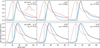 |
Fig. 9 Comparison of azimuthally averaged radial profiles from the 12CO emission (in dotted red), dust continuum emission (in dashed gray), and gas density profile from each simulation setup (in solid blue), calculated as the median from the last 1000 orbits. The value of abin is calculated for each simulation to match the peak density position with the peak brightness position of the dust continuum. The values for ebin increase from left to right, and each row has a constant disk aspect ratio. The average radial resolution of the 12CO and dust continuum are shown in the upper left panel, with Gaussians of the same colors. A dashed vertical line marks the position of the simulated planet. |
5.3. Cavity edge and ring morphology
As shown in Figs. 5 and 9, changing ebin and disk aspect ratios can induce different rings morphologies, as they differ in eccentricity, azimuthal symmetry, radial extent, and density distribution. Observationally constraining of the orbital parameters of the CS Cha binary stars will greatly reduce the degeneracy of the parameter space, as different binary eccentricities will not need to be sampled and the location of the ring peak and the ring width will also become quantities that can be compared among the observations and simulations. Additional observations of CS Cha in longer wavelengths such as 1.3 mm or 3 mm would allow us to test the azimuthal brightness variation along the ring in optically thinner emission, thus increasing the constrains in the proposed planet.
Observations of the disk in scattered light emission have found the cavity edge (if any) to be hidden by the corona-graph of SPHERE, therefore setting an upper limit of 15.6 au (Ginski et al. 2018). This value differs from the temperature peak at 21.6 au that we observe in the 12CO emission, which is most likely the location of the gas cavity inner edge. The difference between those measurements is an additional constrain for the possible planet mass, and the disk physical conditions. For the same ebin, different disk aspect ratios will also modify the shape of the ring inner edge, depleting the material closer or farther from the star, as shown in Fig. 9. To compare the observed profiles to the simulations, we scaled the value of abin such that the peak density position matches with the peak brightness of the dust continuum. This scaling is made under the same assumptions discussed in Sect. 5.2, which is that the brightness peak of the dust continuum will trace the dust density maxima and it will coincide with the gas density maxima of the simulations.
The small μm-sized grains traced by the scattered light images could be getting through the planet orbit via streamers, which connect the main circumbinary ring to the binaries, and replenish their circumstellar disks. In fact, Fig. 9 shows that the simulated gas is not always depleted at the planet location, especially in the setups with h/r = 0.05. The small grains coupled to the gas at the planet orbit location could contribute to the difference in cavity size when observed with different tracers. Interestingly, when the semi-major axis of the planet is scaled from abin to au, all of our simulations locate the planet almost at the same position as the 12CO peak brightness, which probably coincides with the cavity edge, where the 12CO reaches its highest temperature. Follow-up observations with alternative molecular lines, in combination with the accurate determination of the binaries orbits, would set even stronger constrains over the disk physical conditions and the candidate planet mass.
Finally, our work shows the feasibility of applying visibilities modeling with more than one eccentricity. The problem of analytically describing a coordinate system with variable eccentricity as a function of distance can be solved by approximating the emission with multiple components at different distances and eccentricities. While challenging, a combination of such approach with the visibilities modeling of the 12CO emission would overcome the limitations related to image reconstruction with synthesized beam convolution and possibly recover a precise description of the cavity inner edge morphology, location, and eccentricity, as we did for the dust continuum emission.
6. Conclusions
This work presents an analysis of the high angular resolution (≈30 × 46 mas) observations at 0.87 mm of the CS Cha system, composed of a spectroscopic binary (usually referred just as CS Cha) and a co-moving companion at 1.3″ known as CS Cha B (Ginski et al. 2018; Haffert et al. 2020). Our observations do not detect any significant emission from the expected position of CS Cha B, neither in the dust continuum emission or 12CO. We set an upper limit for its disk 0.87 mm continuum emission to be 35.4 µJy, which is the 3σ limit in the image generated with a robust parameter of 1.0.
The circumbinary disk resolves into a single ring, which has a peak in the dust continuum emission at 35 au and 22 au in the 12CO J:3–2 transition. Both the dust and gas emission show evidence of non-circular orbits, which is expected for circumbinary disks. The eccentricity in the dust continuum is constrained by visibility modeling, and we find the peak of the ring to have an eccentricity of 0.039 and the contrast between the brightest and dimmest part along the peak ring to be at most 9%.
From our simulations of circumbinary disks, we find that including a Saturn-mass planet is in better agreement with the observations compared to the disk with no planet, as it can reproduce the low eccentricity and low azimuthal contrast over the ring. Even though it is possible to achieve low disk eccentricities without the need of a planet, the azimuthal symmetry of the disks is only achieved when a planet is present. Additional deep observations of other circumbinary disks could reveal if there is a difference within the circumbinary disks population between disks that do or do not host a gap-opening planet within the cavity.
The accurate determination of the orbital parameters of the CS Cha binary would unlock several additional observables that could be directly compared to the simulations, such as the ring location, ring morphology, and outer-disk radius, which are only measured in binary-separation units in the current simulations.
Acknowledgments.
We would like to dedicate this work to the memory of Willy Kley, who passed away during the development of this paper. We are grateful for his help and advice. The authors thank the anonymous referee for providing a constructive and detailed report. N.K. and P.P. acknowledges support provided by the Alexander von Humboldt Foundation in the framework of the Sofja Kovalevskaja Award endowed by the Federal Ministry of Education and Research. Anna Penzlin was funded by grant KL 650/26-2 from the German Research Foundation (DFG). This project has received funding from the European Research Council (ERC) under the European Union’s Horizon 2020 research and innovation programme (grant agreement No. 101002188). L.P. and A.B. acknowledges support by ANID, “Millennium Science Initiative Program” NCN19_171. A.B. also acknowledges ANID BASAL project FB210003 and Fondecyt (grant 1190748), and L.P. gratefully acknowledges support by the ANID BASAL projects ACE210002 and FB210003. S.P. acknowledges support from FONDECYT grant 1191934 and ANID – Millennium Science Initiative Program – Center Code NCN2021_080. This paper makes use of the following ALMA data: ADS/JAO.ALMA#2017.1.00969.S. ALMA is a partnership of ESO (representing its member states), NSF (USA) and NINS (Japan), together with NRC (Canada), MOST and ASIAA (Taiwan), and KASI (Republic of Korea), in cooperation with the Republic of Chile. The Joint ALMA Observatory is operated by ESO, AUI/NRAO and NAOJ.
Appendix A Additional figures
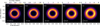 |
Fig. A.1 CS Cha dust continuum emission, as imaged with different robust parameters. The size of the synthesized beams are shown in the bottom left corner of each panel. |
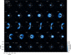 |
Fig. A.2 12CO Channel maps of CS Cha, generated with a robust parameter of 0.0. The velocity of each channel is shown in the upper right corner. The contours are the 5σ level of the continuum image generated with a robust parameter of 0.0. Lower left panel: Scale bar represents 20 au at the distance of the source, and ellipse represents the beam size for all the images. |
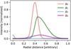 |
Fig. A.3 Schematic profile of the components considered in our uv modeling. |
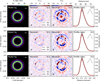 |
Fig. A.4 Best solutions for the dust continuum emission generated with the Models 2g, 3g and 4g. Left panel shows the best model, and middle panels shows the residuals left by the best model after being imaged with different robust parameters, shown in the upper right corned. Right panel shows the intensity profile of the model obtained from tclean (in dashed black) and the best respective model (in red). |
References
- Andrews, S. M., Rosenfeld, K. A., Kraus, A. L., & Wilner, D. J. 2013, ApJ, 771, 129 [Google Scholar]
- Andrews, S. M., Elder, W., Zhang, S., et al. 2021, ApJ, 916, 51 [NASA ADS] [CrossRef] [Google Scholar]
- Ansdell, M., Williams, J. P., van der Marel, N., et al. 2016, ApJ, 828, 46 [Google Scholar]
- Armstrong, D. J., Osborn, H. P., Brown, D. J. A., et al. 2014, MNRAS, 444, 1873 [CrossRef] [Google Scholar]
- Artymowicz, P., & Lubow, S. H. 1994, ApJ, 421, 651 [Google Scholar]
- Ataiee, S., Pinilla, P., Zsom, A., et al. 2013, A&A, 553, A3 [Google Scholar]
- Bate, M. R. 2018, MNRAS, 475, 5618 [Google Scholar]
- Bayo, A., Joergens, V., Liu, Y., et al. 2017, ApJ, 841, L11 [Google Scholar]
- Benisty, M., Bae, J., Facchini, S., et al. 2021, ApJ, 916, L2 [NASA ADS] [CrossRef] [Google Scholar]
- Benítez-Llambay, P., & Masset, F. S. 2016, ApJS, 223, 11 [Google Scholar]
- Beuzit, J. L., Vigan, A., Mouillet, D., et al. 2019, A&A, 631, A155 [NASA ADS] [CrossRef] [EDP Sciences] [Google Scholar]
- Birnstiel, T., Dullemond, C. P., & Pinilla, P. 2013, A&A, 550, A8 [NASA ADS] [CrossRef] [EDP Sciences] [Google Scholar]
- Birnstiel, T., Fang, M., & Johansen, A. 2016, Space Sci. Rev., 205, 41 [Google Scholar]
- Booth, M., Schulz, M., Krivov, A. V., et al. 2021, MNRAS, 500, 1604 [Google Scholar]
- Cuello, N., Dipierro, G., Mentiplay, D., et al. 2019, MNRAS, 483, 4114 [Google Scholar]
- Czekala, I., Loomis, R. A., Teague, R., et al. 2021, ApJS, 257, 2 [NASA ADS] [CrossRef] [Google Scholar]
- de Juan Ovelar, M., Pinilla, P., Min, M., Dominik, C., & Birnstiel, T. 2016, MNRAS, 459, L85 [NASA ADS] [CrossRef] [Google Scholar]
- Doyle, L. R., Carter, J. A., Fabrycky, D. C., et al. 2011, Science, 333, 1602 [NASA ADS] [CrossRef] [Google Scholar]
- Dvorak, R. 1986, A&A, 167, 379 [NASA ADS] [Google Scholar]
- Espaillat, C., Calvet, N., D’Alessio, P., et al. 2007, ApJ, 664, L111 [NASA ADS] [CrossRef] [Google Scholar]
- Espaillat, C., Furlan, E., D’Alessio, P., et al. 2011, ApJ, 728, 49 [NASA ADS] [CrossRef] [Google Scholar]
- Foreman-Mackey, D., Hogg, D. W., Lang, D., & Goodman, J. 2013, PASP, 125, 306 [Google Scholar]
- Gaia Collaboration (Prusti, T., et al.) 2016, A&A, 595, A1 [NASA ADS] [CrossRef] [EDP Sciences] [Google Scholar]
- Gaia Collaboration (Brown, A. G. A., et al.) 2021, A&A, 649, A1 [NASA ADS] [CrossRef] [EDP Sciences] [Google Scholar]
- Gauvin, L. S., & Strom, K. M. 1992, ApJ, 385, 217 [NASA ADS] [CrossRef] [Google Scholar]
- Ginski, C., Benisty, M., van Holstein, R. G., et al. 2018, A&A, 616, A79 [NASA ADS] [CrossRef] [EDP Sciences] [Google Scholar]
- Guenther, E. W., Esposito, M., Mundt, R., et al. 2007, A&A, 467, 1147 [CrossRef] [EDP Sciences] [Google Scholar]
- Haffert, S. Y., van Holstein, R. G., Ginski, C., et al. 2020, A&A, 640, L12 [EDP Sciences] [Google Scholar]
- Hendler, N., Pascucci, I., Pinilla, P., et al. 2020, ApJ, 895, 126 [Google Scholar]
- Henning, T., Pfau, W., Zinnecker, H., & Prusti, T. 1993, A&A, 276, 129 [NASA ADS] [Google Scholar]
- Hildebrand, R. H. 1983, QJRAS, 24, 267 [NASA ADS] [Google Scholar]
- Hirsh, K., Price, D. J., Gonzalez, J.-F., Ubeira-Gabellini, M. G., & Ragusa, E. 2020, MNRAS, 498, 2936 [NASA ADS] [CrossRef] [Google Scholar]
- Holman, M. J., & Wiegert, P. A. 1999, AJ, 117, 621 [Google Scholar]
- Jorsater, S., & van Moorsel, G. A. 1995, AJ, 110, 2037 [Google Scholar]
- Kim, K. H., Watson, D. M., Manoj, P., et al. 2009, ApJ, 700, 1017 [NASA ADS] [CrossRef] [Google Scholar]
- Kley, W., & Haghighipour, N. 2014, A&A, 564, A72 [NASA ADS] [CrossRef] [EDP Sciences] [Google Scholar]
- Kley, W., Thun, D., & Penzlin, A. B. T. 2019, A&A, 627, A91 [NASA ADS] [CrossRef] [EDP Sciences] [Google Scholar]
- Kostov, V. B., Orosz, J. A., Feinstein, A. D., et al. 2020, AJ, 159, 253 [Google Scholar]
- Kurtovic, N. T., Pérez, L. M., Benisty, M., et al. 2018, ApJ, 869, L44 [Google Scholar]
- Lubow, S. H. 1991, ApJ, 381, 259 [Google Scholar]
- Luhman, K. L. 2007, ApJS, 173, 104 [Google Scholar]
- MacFadyen, A. I., & Milosavljević, M. 2008, ApJ, 672, 83 [Google Scholar]
- Manara, C. F., Testi, L., Natta, A., et al. 2014, A&A, 568, A18 [NASA ADS] [CrossRef] [EDP Sciences] [Google Scholar]
- Manara, C. F., Tazzari, M., Long, F., et al. 2019, A&A, 628, A95 [NASA ADS] [CrossRef] [EDP Sciences] [Google Scholar]
- Marino, S., Yelverton, B., Booth, M., et al. 2019, MNRAS, 484, 1257 [NASA ADS] [CrossRef] [Google Scholar]
- Martin, D. V. 2019, MNRAS, 488, 3482 [NASA ADS] [CrossRef] [Google Scholar]
- Martin, D. V., & Triaud, A. H. M. J. 2014, A&A, 570, A91 [NASA ADS] [CrossRef] [EDP Sciences] [Google Scholar]
- Meschiari, S. 2012, ApJ, 752, 71 [NASA ADS] [CrossRef] [Google Scholar]
- Miranda, R., & Lai, D. 2015, MNRAS, 452, 2396 [Google Scholar]
- Muñoz, D. J., & Lithwick, Y. 2020, ApJ, 905, 106 [CrossRef] [Google Scholar]
- Musso Barcucci, A., Cugno, G., Launhardt, R., et al. 2019, A&A, 631, A84 [NASA ADS] [CrossRef] [EDP Sciences] [Google Scholar]
- Nguyen, D. C., Brandeker, A., van Kerkwijk, M. H., & Jayawardhana, R. 2012, ApJ, 745, 119 [Google Scholar]
- Norfolk, B. J., Maddison, S. T., Pinte, C., et al. 2021, MNRAS, 502, 5779 [Google Scholar]
- Paardekooper, S.-J., Leinhardt, Z. M., Thébault, P., & Baruteau, C. 2012, ApJ, 754, L16 [NASA ADS] [CrossRef] [Google Scholar]
- Penzlin, A. B. T., Ataiee, S., & Kley, W. 2019, A&A, 630, L1 [NASA ADS] [CrossRef] [EDP Sciences] [Google Scholar]
- Penzlin, A. B. T., Kley, W., & Nelson, R. P. 2021, A&A, 645, A68 [NASA ADS] [CrossRef] [EDP Sciences] [Google Scholar]
- Pérez, S., Marino, S., Casassus, S., et al. 2019, MNRAS, 488, 1005 [Google Scholar]
- Phuong, N. T., Dutrey, A., Diep, P. N., et al. 2020, A&A, 635, A12 [NASA ADS] [CrossRef] [EDP Sciences] [Google Scholar]
- Pierens, A., & Nelson, R. P. 2007, A&A, 472, 993 [NASA ADS] [CrossRef] [EDP Sciences] [Google Scholar]
- Pierens, A., & Nelson, R. P. 2008, A&A, 483, 633 [NASA ADS] [CrossRef] [EDP Sciences] [Google Scholar]
- Pierens, A., McNally, C. P., & Nelson, R. P. 2020, MNRAS, 496, 2849 [CrossRef] [Google Scholar]
- Pinilla, P., Birnstiel, T., Ricci, L., et al. 2012, A&A, 538, A114 [NASA ADS] [CrossRef] [EDP Sciences] [Google Scholar]
- Pinilla, P., Natta, A., Manara, C. F., et al. 2018, A&A, 615, A95 [NASA ADS] [CrossRef] [EDP Sciences] [Google Scholar]
- Pinilla, P., Kurtovic, N. T., Benisty, M., et al. 2021, A&A, 649, A122 [NASA ADS] [CrossRef] [EDP Sciences] [Google Scholar]
- Ragusa, E., Alexander, R., Calcino, J., Hirsh, K., & Price, D. J. 2020, MNRAS, 499, 3362 [NASA ADS] [CrossRef] [Google Scholar]
- Ragusa, E., Fasano, D., Toci, C., et al. 2021, MNRAS, 507, 1157 [NASA ADS] [CrossRef] [Google Scholar]
- Ribas, Á., Bouy, H., Merín, B., et al. 2016, MNRAS, 458, 1029 [NASA ADS] [CrossRef] [Google Scholar]
- Rodriguez, J. E., Loomis, R., Cabrit, S., et al. 2018, ApJ, 859, 150 [Google Scholar]
- Rosenfeld, K. A., Chiang, E., & Andrews, S. M. 2014, ApJ, 782, 62 [Google Scholar]
- Schmid, H. M., Bazzon, A., Roelfsema, R., et al. 2018, A&A, 619, A9 [NASA ADS] [CrossRef] [EDP Sciences] [Google Scholar]
- Shakura, N. I., & Sunyaev, R. A. 1973, A&A, 24, 337 [NASA ADS] [Google Scholar]
- Teague, R. 2019a, J. Open Source Softw., 4, 1220 [Google Scholar]
- Teague, R. 2019b, RNAAS, 3, 74 [NASA ADS] [Google Scholar]
- Teague, R., & Foreman-Mackey, D. 2018, RNAAS, 2, 173 [NASA ADS] [Google Scholar]
- Thun, D., & Kley, W. 2018, A&A, 616, A47 [NASA ADS] [CrossRef] [EDP Sciences] [Google Scholar]
- Thun, D., Kley, W., & Picogna, G. 2017, A&A, 604, A102 [NASA ADS] [CrossRef] [EDP Sciences] [Google Scholar]
- Tiede, C., Zrake, J., MacFadyen, A., & Haiman, Z. 2020, ApJ, 900, 43 [NASA ADS] [CrossRef] [Google Scholar]
- Tripathi, A., Andrews, S. M., Birnstiel, T., & Wilner, D. J. 2017, ApJ, 845, 44 [Google Scholar]
- Virtanen, P., Gommers, R., Oliphant, T. E., et al. 2020, Nature Methods, 17, 261 [CrossRef] [Google Scholar]
Check https://casa.nrao.edu/docs/taskref/tclean-task.html for a description of the parameters.
The term “uv” in this work is used to refer to the visibility plane.
All Tables
Best parameters from the kinematic fitting with eddy to the image generated with a robust parameter of 0.0.
Eccentricity and semi-major axis of the cavity edge (ecav, acav), peak density (epeak, apeak), and planetary orbit (epl, apl).
All Figures
|
Fig. 1 Reconstructed images of dust continuum emission and 12CO. From left to right: dust continuum emission from CS Cha imaged with a robust parameter of −0.5, moment 0 and moment 1 of the 12CO imaged with a robust of −0.2, and radial profiles for the continuum and 12CO emission calculated by deprojecting the images with the inclination and position angle of Model 2e (see Sect. 3.3). The ellipse in the left bottom corner of the panels represents the synthesized beam of the images, which is 30 * 46 mas for the dust continuum and 80 * 77 mas for the 12CO. The scale bar in the top right of the first panel represents 20 au at the distance of the source. The Gaussians in the right panel represent the average radial resolution of the profiles, and in the same panel, the colored region in the profiles represent the 1 σ dispersion at each radial location. |
| In the text | |
|
Fig. 2 High-sensitivity millimeter emission images of CS Cha. Upper panel: dust continuum image generated with a robust parameter of 1.0. The color scale is linear and has been saturated to show the emission between 0 and 5σcont, with σcont = 11.8 μJy beam−1 being the rms of this image. A box of 0.2″ per side is centered at the expected location of CS ChaB. The beam size is 105 × 75 mas, and is shown in the lower left corner of the figure. The scale bar at the top right represents 20 au. Lower panel: 12CO emission image generated with a robust parameter of 1.2, after stacking all the channel maps between −24 and 24 kms−1 around the rest frame. The beam size is 148 × 97 mas, and is shown in the lower left corner of the figure. The color scale is linear and has been saturated to show the emission between 0 and 5σ12CO, with σ12CO = 1.4 mJy beam−1 being the rms of this image. |
| In the text | |
|
Fig. 3 Best solution for the dust continuum emission generated using the Model 2e, which considers two eccentricities for the disk components. Upper row: left panel shows the synthetic image of the best model found. Middle panels show how this model would have been observed by ALMA with two different robust parameters, comparable to the images from Fig. A.l. Right panel shows the radial profile obtained from the beam convolved images generated with a robust parameter of 0.0, and the average beam resolution shown with a Gaussian in gray. Lower row: middle panels show the residuals left by the best model, imaged with two different robust parameters shown in the upper left corner. Right panel shows the intensity profile of the model obtained from tclean and the best Model 2e (not convolved by beam). |
| In the text | |
|
Fig. 4 CS Cha gas emission and kinematics. Upper row: 12CO moment 0, the best model using the geometry recovered from the kinematic fit, and the residuals. Scale bar represents 20 au at the distance of the source. Lower row: 12CO peak velocity in the line of sight, with the best model calculated with the parameters from Table 2, and the residuals. The dashed line shows the mask used for the fit. |
| In the text | |
|
Fig. 5 Gas surface density after 100 000 binary orbits in each setup. Distance is in binary separations and the color scale is normalized to the maximum of each image. Panels on the left and right show the setups with h/r = 0.03 and h/r = 0.05 respectively. In each panel, the columns show the setups with the same binary eccentricity, being 0.15, 0.25, and 0.35 from left to right. The upper row of each panel contains the setups with no planet, and the lower row the setups with planet. A white dashed line shows the best cavity fit, while the black dashed line shows the best peak ring fit. A white triangle is used to show the position of the planet. |
| In the text | |
|
Fig. 6 Eccentricity and semi-major axis for the cavity (ecav, acav) as a function of time in binary orbits. Each panel contains the simulations of the three different ebin for the binaries, and a single aspect ratio, displayed in the left-side together with the line-style legend. |
| In the text | |
|
Fig. 7 Eccentricity and semi-major axis for the peak density ring (epeak, apeak) as a function of time in binary orbits. Each panel contains the simulations of the three different ebin values for the binaries and a single aspect ratio, displayed in the left-side together with the line-style legend. |
| In the text | |
|
Fig. 8 Planet’s semi-major axis and eccentricity as a function of time (in binary orbits) in the upper and lower panel row, respectively. The upper right number in each plot indicates the eccentricity of the binaries. The dashed vertical curve indicates the position of the 50 000 binary orbits, after which the planet has converged to its equilibrium orbit. The median semi-major axis for the planet orbit after convergence is indicated with a dotted line. |
| In the text | |
|
Fig. 9 Comparison of azimuthally averaged radial profiles from the 12CO emission (in dotted red), dust continuum emission (in dashed gray), and gas density profile from each simulation setup (in solid blue), calculated as the median from the last 1000 orbits. The value of abin is calculated for each simulation to match the peak density position with the peak brightness position of the dust continuum. The values for ebin increase from left to right, and each row has a constant disk aspect ratio. The average radial resolution of the 12CO and dust continuum are shown in the upper left panel, with Gaussians of the same colors. A dashed vertical line marks the position of the simulated planet. |
| In the text | |
|
Fig. A.1 CS Cha dust continuum emission, as imaged with different robust parameters. The size of the synthesized beams are shown in the bottom left corner of each panel. |
| In the text | |
|
Fig. A.2 12CO Channel maps of CS Cha, generated with a robust parameter of 0.0. The velocity of each channel is shown in the upper right corner. The contours are the 5σ level of the continuum image generated with a robust parameter of 0.0. Lower left panel: Scale bar represents 20 au at the distance of the source, and ellipse represents the beam size for all the images. |
| In the text | |
|
Fig. A.3 Schematic profile of the components considered in our uv modeling. |
| In the text | |
|
Fig. A.4 Best solutions for the dust continuum emission generated with the Models 2g, 3g and 4g. Left panel shows the best model, and middle panels shows the residuals left by the best model after being imaged with different robust parameters, shown in the upper right corned. Right panel shows the intensity profile of the model obtained from tclean (in dashed black) and the best respective model (in red). |
| In the text | |
Current usage metrics show cumulative count of Article Views (full-text article views including HTML views, PDF and ePub downloads, according to the available data) and Abstracts Views on Vision4Press platform.
Data correspond to usage on the plateform after 2015. The current usage metrics is available 48-96 hours after online publication and is updated daily on week days.
Initial download of the metrics may take a while.