| Issue |
A&A
Volume 664, August 2022
|
|
|---|---|---|
| Article Number | A167 | |
| Number of page(s) | 25 | |
| Section | Extragalactic astronomy | |
| DOI | https://doi.org/10.1051/0004-6361/202142593 | |
| Published online | 25 August 2022 | |
Photometric properties of nuclear star clusters and their host galaxies in the Fornax cluster⋆
1
Space Physics and Astronomy Research Unit, University of Oulu, Pentti Kaiteran katu 1, 90014 Oulu, Finland
e-mail: hung-shuo.su@oulu.fi
2
Finnish Centre of Astronomy with ESO (FINCA), Vesilinnantie 5, University of Turku, 20014 Turku, Finland
3
Specim, Spectral Imaging Ltd., Elektroniikkatie 13, 90590 Oulu, Finland
4
Kapteyn Institute, University of Groningen, Landleven 12, 9747 AD Groningen, The Netherlands
Received:
5
November
2021
Accepted:
27
May
2022
Aims. We aim to investigate the relations between nuclear star clusters (NSCs) and their host galaxies and to offer a comparison between the structural properties of nucleated and non-nucleated galaxies. We also address the environmental influences on the nucleation of galaxies in the Fornax main cluster and the Fornax A group.
Methods. We selected 557 galaxies (105.5 M⊙ < M*, galaxy < 1011.5 M⊙) for which structural decomposition models and non-parametric morphological measurements are available from our previous work. We determined the nucleation of galaxies based on a combination of visual inspection of galaxy images and residuals from multi-component decomposition models, as well as using a model selection statistic, the Bayesian information criterion (BIC), to avoid missing any faint nuclei. We also tested the BIC as an unsupervised method to determine the nucleation of galaxies. We characterised the NSCs using the nucleus components from the multi-component models conducted in the g′, r′, and i′ bands.
Results. Overall, we find a dichotomy in the properties of nuclei that reside in galaxies more or less massive than M*, galaxy ≈ 108.5 M⊙. In particular, we find that the nuclei tend to be bluer than their host galaxies and follow a scaling relation of  for M*, galaxy < 108.5 M⊙. In galaxies with M*, galaxy > 108.5 M⊙, we find redder nuclei compared to the host galaxy, which follows M*, nuc ∝ M*, galaxy. Comparing the properties of nucleated and non-nucleated early-type galaxies, we find that nucleated galaxies tend to be redder in global (g′−r′) colour, have redder outskirts relatively to their own inner regions (Δ(g′−r′)), are less asymmetric (A), and exhibit less scatter in the brightest second-order moment of light (M20) than their non-nucleated counterparts at a given stellar mass. However, with the exception of Δ(g′−r′) and the Gini coefficient (G), we do not find any significant correlations with cluster-centric distance. Yet, we find the nucleation fractions to be typically higher in the Fornax main cluster than in the Fornax A group, and that the nucleation fraction is highest towards the centre of their respective environments. Additionally, we find that the observed ultra-compact dwarf (UCD) fraction (i.e. the number of UCDs over the number of UCDs and nucleated galaxies) in Fornax and Virgo peaks at the cluster centre and is consistent with the predictions from simulations. Lastly, we find that the BIC can recover our labels of nucleation up to an accuracy of 97% without interventions.
Conclusions. The different trends in NSC properties suggest that different processes are at play at different host stellar masses. A plausible explanation is that the combination of globular cluster in-spiral and in situ star formation play a key role in the build-up of NSCs. In addition, the environment is clearly another important factor in the nucleation of galaxies, particularly at the centre of the cluster where the nucleation and UCD fractions peak. Nevertheless, the lack of significant correlations with the structures of the host galaxies is intriguing. Finally, our exploration of the BIC as a potential method of determining nucleation have applications for large-scale future surveys, such as Euclid.
Key words: galaxies: nuclei / galaxies: clusters: individual: Fornax / galaxies: groups: individual: Fornax A / galaxies: structure / galaxies: dwarf / galaxies: photometry
Full Tables 1 and 2 are only available at the CDS via anonymous ftp to cdsarc.u-strasbg.fr (130.79.128.5) or via http://cdsarc.u-strasbg.fr/viz-bin/cat/J/A+A/664/A167
© A. H. Su et al. 2022
 Open Access article, published by EDP Sciences, under the terms of the Creative Commons Attribution License (https://creativecommons.org/licenses/by/4.0), which permits unrestricted use, distribution, and reproduction in any medium, provided the original work is properly cited.
This article is published in open access under the Subscribe-to-Open model. Subscribe to A&A to support open access publication.
1. Introduction
The nucleation of galaxies typically refers to a bright compact object located at the central region of the galaxy, which is composed of a massive stellar cluster also known as a nuclear star cluster (NSC). These objects typically appear as an excess of light in the innermost part of the surface brightness profiles of galaxies. Although nuclei typically only take up a few percent of the total light of a given galaxy (Côté et al. 2006; Turner et al. 2012; Georgiev et al. 2016; Sánchez-Janssen et al. 2019a), their prevalence across galaxies in our local Universe cannot be underestimated. Galaxies that host nuclei can exhibit a range of properties, from low to high stellar masses and between early- and late-type galaxies (see e.g., Georgiev et al. 2016; Neumayer et al. 2020). Even our own Milky Way has been observed to host an NSC (see Fritz et al. 2016 and references therein). Furthermore, given the proximity of nuclei to the centre of the galaxies, it is possible that there is some interplay with the central black holes in larger mass galaxies, which have comparable masses (Côté et al. 2006; Antonini 2013; Arca-Sedda et al. 2016; Greene et al. 2020).
How NSCs form and grow is an active topic of study. Recent studies attribute two main mechanisms to the growth of NSCs. The first is the in-spiral of globular clusters (GCs) towards the centre of a galaxy due to dynamical friction (Tremaine et al. 1975; Capuzzo-Dolcetta 1993; Oh & Lin 2000; Lotz et al. 2001). Observationally, there are several works that found links between the GCs and NSCs of early-type galaxies, such as the lack of GCs in the central regions where NSCs reside (Lotz et al. 2001) and the similarity in NSC and GC occupation fraction (Sánchez-Janssen et al. 2019a). This mechanism appears to dominate for lower mass galaxies (M* ≲ 109 M⊙), given the similarity between the predicted and observed NSC-to-host stellar mass scaling relations (Antonini 2013; Gnedin et al. 2014; Neumayer et al. 2020). Another mechanism is the in situ star formation from gas in the central region of a galaxy (Seth et al. 2006). For example, the compression of gas in the central region of galaxies via tidal compression (Emsellem & van de Ven 2008), that fuelled by gas infall (Maciejewski 2004; Hunt et al. 2008; Emsellem et al. 2015), coalescence of star forming clumps (Bekki et al. 2006; Bekki 2007), or that due to magnetorotational instability (Milosavljević 2004). Whilst the timescales vary between the aforementioned processes, in situ star formation is considered to be the dominant channel of NSC growth for massive galaxies (M* ≳ 109 M⊙; e.g., Paudel et al. 2011; Johnston et al. 2020; Fahrion et al. 2021; Pinna et al. 2021). Combining both cluster in-spiral and in situ star formation, as well as effects from black holes, Antonini et al. (2015) found that NSCs tend to dominate over the central black holes for dwarfs, and vice versa for massive galaxies (Graham 2016).
In terms of the stellar population of NSCs, one NSC that has been observed in great detail is that of the Milky Way. The Milky Way NSC has a half-light radius of 7 ± 2 pc and a mass of 4.2 × 10⁷ M⊙ (Fritz et al. 2016). Analyses from infrared surveys suggest that stars within the central parsec tend to be old (9 ± 2 Gyr; Genzel et al. 2010, their Sect. 6.1), similarly to those from the Galactic bulge. Stars belonging to the NSC (and its periphery) tend to be metal-rich (Schultheis et al. 2019; Thorsbro et al. 2020), although there is evidence that young (Feldmeier-Krause et al. 2015) and metal-poor (Ryde et al. 2016; Feldmeier-Krause et al. 2017) stars are also present. In principle, the metal-poor stars could have come from the in-spiral of GCs. However, a young stellar population is unlikely to originate from GCs and points to in situ star formation (Nishiyama et al. 2016). Another hypothetical scenario is the infall of young stellar clusters into the NSC, which is unlikely in the case of the Milky Way due to the predominantly old stellar population in the inner Galactic bulge (Nogueras-Lara et al. 2018) and nuclear stellar disc (NSD, Nogueras-Lara et al. 2020)1.
For extragalactic NSCs, stars can no longer be resolved individually, which hampers efforts to study the age and metallicity distributions. Nonetheless, space-based observations with high spatial resolution can still resolve NSCs as a whole, which has led to several studies of NSC luminosity functions, nucleation fractions, scaling relations, and colours for galaxies in the Virgo (Côté et al. 2006; Ferrarese et al. 2006), Fornax (Turner et al. 2012), and Coma (den Brok et al. 2014) clusters. More recently, spectroscopic studies using integral field units (IFUs) have uncovered a mix of ages and metallicities for NSCs in galaxies in the Fornax cluster (e.g., Johnston et al. 2020; Fahrion et al. 2021). The varying star formation histories suggest that both cluster in-spiral and in situ star formation play a role in the formation and growth of most NSCs, depending on the host galaxy mass.
A wealth of photometric data on nucleated galaxies have come from recent ground-based, deep, and wide-field observations in cluster and group environments (e.g., FDS, Iodice et al. 2016; NGVS, Ferrarese et al. 2012; NGFS, Muñoz et al. 2015; ELVES, Carlsten et al. 2021; MATLAS, Habas et al. 2020). In particular, Venhola et al. (2019) found that nucleated and non-nucleated dwarfs in the Fornax cluster can show significantly different luminosity functions and structural scaling relations. For dwarfs in the Virgo cluster, Sánchez-Janssen et al. (2019a) found that the nucleus occupation fraction peaks at M* ≈ 109 M⊙. Recently, Su et al. (2021) conducted multi-component decompositions on both the dwarfs (from Venhola et al. 2018) and massive galaxies (from Iodice et al. 2019; Raj et al. 2019, 2020) in the Fornax main cluster and the nearby Fornax A group. The multi-component decompositions, which included the nucleus components, provide structural parameters in multiple bands, and which we made use of in this work.
This paper is structured as follows. We describe the data and the sample we used in Sect. 2, including our label of nucleation for each galaxy in our sample. In Sect. 5, we discuss how we tested methods of automatically selecting the most appropriate decomposition models and applied them to determine the nucleation of galaxies. In Sect. 3, we show the nucleation fraction as a function of the environment (i.e. between the Fornax main cluster and Fornax A group). In Sect. 4, we present the properties of nucleated and non-nucleated galaxies in our sample and compare them. In Sect. 6, we compare the nucleated galaxies to mechanisms of NSC growth from the literature, discuss the role of the environment on the structural properties of our sample galaxies, and compare the nuclei to ultra-compact dwarfs (UCDs). Finally, we summarise our results in Sect. 7. Throughout this study, we used a distance modulus of 31.5 mag, which is equivalent to a distance of 20 Mpc (Blakeslee et al. 2009). At this distance, 1 arcsec corresponds to ∼0.097 kpc.
2. Sample
2.1. Data
We utilised data from the Fornax Deep Survey (FDS), a combination of two guaranteed time observation surveys with the OmegaCAM instrument (Kuijken et al. 2002) at the VLT Survey Telescope (VST): FOCUS (P.I. R. F. Peletier) and VEGAS (P.I. E. Iodice, Capaccioli et al. 2015). The FDS covers 26 deg2 around the Fornax main cluster and Fornax A group in u′, g′, r′, and i′ bands, with an average seeing full width at half maximum (FWHM) of 1.2 arcsec, 1.1 arcsec, 1.0 arcsec, and 1.0 arcsec, respectively. The images have a pixel scale of 0.2 arcsec pix−1. In terms of the data depth, the 1σ signal-to-noise per pixel can be converted to surface brightness of 26.6, 26.7, 26.1, 25.5 mag arcsec−2 for u′, g′, r′, and i′ bands, respectively. Alternatively, when averaged over an area of 1 arcsec2, the surface brightnesses correspond to 28.3, 28.4, 27.8, and 27.2 mag arcsec−2 for u′, g′, r′, and i′ bands, respectively. The images are calibrated in the AB magnitude system. The full observation strategy can be found in Iodice et al. (2016), and the reduction steps can be found in Venhola et al. (2018). The FDS data can be obtained from the ESO Science Archive (Peletier et al. 2020).
To tackle the topic of galaxy nucleation, we made use of the analysis of FDS galaxies from Su et al. (2021), which consists of 582 galaxies (dwarfs from FDSDC and Venhola et al. 2018, and massive galaxies from Iodice et al. 2019 and Raj et al. 2019, 2020) in the Fornax main cluster and Fornax A group (see Fig. 1). These galaxies were deemed likely cluster and group members based on the selection cuts in Venhola et al. (2018). To briefly describe the data preprocessing steps from Su et al. (2021), postage stamp images for each member galaxy were cut in each band; the images were sky-subtracted using a constant value, except in select cases where a strong gradient requires a plane subtraction; a separate PSF was created for each FDS field by averaging the radial flux profiles of point sources in the field and interpolating, which produced axisymmetric PSFs (for more details see Su et al. 2021, their Sect. 3). The compilation in Su et al. (2021) contains quantities derived from structural decompositions as well as non-parametric morphological indices. The structural decompositions were conducted using GALFIT (Peng et al. 2010), with two types of models for each galaxy: Sérsic+PSF and multi-component. The Sérsic+PSF model fit the unresolved nucleus (if present) with the PSF and the galaxy with a Sérsic function. Constraints were applied such that the integrated magnitude of the nucleus component cannot be fainter than 35 mag. This allowed the Sérsic parameters to remain accurate even for non-nucleated galaxies and prevented GALFIT from failing.
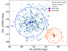 |
Fig. 1. Overview of Fornax galaxies, split between Fornax main cluster (blue) and Fornax A group (orange). The dashed circles denote the virial radius for the Fornax main cluster (∼2 deg = 0.7 Mpc) and the Fornax A group (∼1 deg = 0.35 Mpc) (Drinkwater et al. 2001). The black dots denote galaxies with a nucleus. |
From the multi-component models, we obtain the morphological structures present in the galaxies, such as bulges, bars, discs, and nuclei using the Sérsic, Ferrers, exponential, and PSF functions to model them, respectively, from Su et al. (2021). The multi-component decompositions were first conducted using the r′ band images, with the parameters from each component allowed to vary to determine their best-fit values. To obtain the magnitudes of individual components in the g′ and i′ bands, only the magnitude parameter was allowed to vary for each component, whilst the other parameters were fixed to the best-fit values obtained from the r′ band model. This ensured that an equivalent aperture was used for each galaxy across different bands. In conjunction, the non-parametric morphological indices provide a model-independent perspective of the galaxies, including deviations from smooth, elliptical light distributions. The combination of quantities allows us to probe the properties of the nuclei themselves, along with the properties of the host galaxies. The analyses and relevant images can be found in Su et al. (2021) as well as on our web page2.
The compilation also includes the stellar mass of the galaxies. The stellar mass was estimated using a combination of g′, r′, and i′ band magnitudes and the empirical relation based on Taylor et al. (2011):

where Mr′ is the absolute r′ band total magnitude, and the g′−i′ and r′−i′ are the total colours based on multi-component decompositions (see also Su et al. 2021, their Sect. 5). Moreover, we used the galaxy coordinates to calculate the projected separation of the galaxies to NGC1399 and NGC1316, as proxies for the centre of the Fornax main cluster and Fornax A group environments, respectively. We assigned each galaxy as a member of either the cluster or group environment following Su et al. (2021), and we adopted an early- and late-type classification from Venhola et al. (2018).
2.2. Nucleus detection
The distinction between nucleated and non-nucleated galaxies in Su et al. (2021) was based on the visual identification of components that were then modelled in multi-component decompositions. Whilst this generally worked well for the bright nuclei in our galaxies, it may fail to capture the faintest nuclei. To check that we did not miss any nuclei, we then added a nucleus component to the multi-component decomposition models of all non-nucleated galaxies (i.e. those without a nucleus component in their multi-component models in Su et al. 2021) in our sample and reran the decomposition models via GALFIT. Similarly to the Sérsic+PSF decompositions, we applied a lower limit on the nucleus component, meaning that their integrated magnitude cannot be fainter than 35 mag, otherwise GALFIT would crash for (truly) non-nucleated galaxies.
To evaluate whether the added nucleus component provides an improvement for each galaxy, we used the Bayesian information criterion (BIC; see Schwarz 1978) as a quantitative indicator. The BIC can be formulated (according to Kass & Raftery 1995) as
where k is the number of free parameters (e.g., our Sérsic+PSF model has six free parameters: five from the Sérsic function and one from the PSF function), npix is the number of pixels used in model fitting (excluding masked pixels), and
![$$ \begin{aligned} \chi ^2=\sum _{x}\sum _{{ y}}\frac{\left[O(x,{ y})-M(x,{ y})\right]^2}{\sigma (x,{ y})^2}, \end{aligned} $$](/articles/aa/full_html/2022/08/aa42593-21/aa42593-21-eq4.gif)
where O is the galaxy image, M is the PSF-convolved decomposition model, σ is the uncertainty in the pixels (i.e. sigma image), and x and y denote the pixel index in the x- and y-axes of the images, respectively. In essence, the first term in Eq. (2) describes how well the model fits the data whilst the second term provides a penalty for model complexity, essentially averting models with more components than necessary.
Head et al. (2014) (see also Simard et al. 2011) argued that the pixels in images are not independent due to effects of the PSF. Hence, an estimate of the resolution element is given as the circular area with radius as the half width at half maximum (HWHM) in pixels (i.e. Ares = π HWHM2)3. This modified BIC can be calculated as
The additional Ares term means that, in general, BICres penalises complex models more than the BIC.
To use the BIC for model selection, each model requires its BIC value to be calculated. The model with the lowest BIC is favoured. This can be formulated as ΔBIC = BICno nuc − BICnuc for both BIC and BICres, such that a positive ΔBIC means the nucleated model is preferred. We note that ΔBIC is the key quantity in determining whether a nucleated model is preferred, rather than the BIC itself. In fact, by definition, the χ2 (and hence the BIC) increases with larger image size. Therefore, for a given galaxy model, the BIC for a postage stamp image that contains a large portion of the background sky would be higher than for a postage stamp image that includes less of the sky. However, as the sky region does not affect the decomposition parameters, the increase in the BIC is mainly driven by the change in the image size, which cancels out when the ΔBIC is calculated. We test and confirm that the ΔBIC is insensitive to the image size used, provided that the image includes the entire galaxy.
2.3. Final sample
To summarise the process of deriving our final working sample, we show the steps in Fig. 2. From the compilation sample of 582 galaxies, 25 were removed due to unsatisfactory decomposition models (for more details, see Appendix B and footnote 10 of Su et al. 2021), leaving 557 galaxies, of which 128 were determined as nucleated in Su et al. (2021). Given the greater sensitivity of BIC in detecting faint nuclei over BICres, for each non-nucleated galaxy we calculated the BIC for the original multi-component model and the corresponding model with the added nucleus component. Hence, galaxies that have a positive ΔBIC are potentially nucleated ones, even if they were not treated as nucleated in Su et al. (2021). Of these 103 galaxies, we visually inspected the central 10 arcsec radius of the original galaxy images and residuals (from both types of decomposition models) and found 20 galaxies that, in fact, host a nucleus4. For the purpose of comparing between nucleated and non-nucleated galaxies in this study, we also labelled these 20 galaxies as nucleated. In total, our sample includes 148 nucleated galaxies and 409 non-nucleated galaxies that we used for further analysis.
In Fig. 3 we show the distribution of stellar mass for nucleated and non-nucleated galaxies in our sample. Of the newly identified nuclei, many belong to massive (M* > 109 M⊙) galaxies with additional structures (e.g., bulges and bars). In total, 140 out of 466 early-type galaxies and eight out of 91 late-type galaxies are nucleated. Based on our completeness tests, our nucleus sample should be complete to around M*, nuc ∼ 104.5 M⊙ (see Appendix B for details on the completeness). In Table 1, we present the photometric properties of a few of our galaxies as examples; the full table can be found at the CDS.
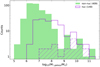 |
Fig. 3. Histograms of host galaxy stellar masses for nucleated (violet) and non-nucleated (green) galaxies in the Fornax main cluster and Fornax A group. The dashed histogram denotes the distribution of newly identified nucleated galaxies (see Sect. 2.3). Bins with widths of 0.5 dex were used. |
Photometric properties of our galaxies.
From detailed inspections, we find that the 83 false positive galaxies (i.e. ΔBIC > 0 but not nucleated; see Fig. 2) broadly fall under one of two types. The first type (type 1) encompasses galaxies that do not host a nucleus but have additional sub-structures in the central regions of the galaxy, such that the inclusion of a nucleus component can reduce the residuals (and hence the corresponding BIC). These sub-structures are generally small deviations from a single Sérsic model (70), with some (12) showing signs of more complex and asymmetric structures (e.g., star-forming clumps, spirals). A few of the galaxies (13) fall into the second type of false positives (type 2). They generally have an unresolved compact object at the centre of their image, but the Sérsic component of the models are clearly off-centre. This can be due to the asymmetric shape of the galaxy on the whole, or the proximity of GCs in the central region of the galaxy. Due to the implied offset of the potential nucleus from the centre of the galaxy, it is somewhat ambiguous whether they are truly NSCs. As such, in these cases we do not label them as nucleated, resulting in their false positive label. In Fig. 4, we show examples of both types of false positives in terms of their images and residuals from multi-component models with and without a nucleus component.
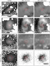 |
Fig. 4. Examples of BIC false positives (i.e. ΔBIC > 0 but no nucleus). We show the images (left) and residuals based on the multi-component model without (centre) and with (right) a nucleus component. The white regions denote masked regions. The images in the first column have widths of 4Re and surface brightness limits from 18–27 mag arcsec2, whereas the residual images have widths of 20 arcsec and are limited from –1 to 1 mag arcsec2 in surface brightness. The red circles have a radius of the average PSF FWHM × 2. The galaxy stellar masses are annotated in the first column. |
The ramification of our false positive classifications is that our nucleation sample is likely biased against clearly off-centred NSCs and, by implication, late types. Of the 83 false positives, we find that 36 are late types and that ten out of 13 type 2 false positives are late types. If we assume that between ten and 36 late-type false positives actually host an offset nucleus, the late-type nucleation fraction would increase from 0.09 (8 out of 91) to between 0.20 and 0.48, with the latter as an upper limit. This would broadly be comparable to the early-type nucleation fraction (≈0.3).
3. Nucleation fraction
The nucleation of galaxies has been observed to depend on both the stellar mass and the environment that the host galaxy resides in (e.g., Binggeli et al. 1987; Côté et al. 2006; Lisker et al. 2007; Sánchez-Janssen et al. 2019a); nucleated galaxies tend to be more massive and reside in denser environments than their non-nucleated counterparts. In this work, we investigated the nucleation fraction as a function of the galaxy stellar mass and the environment, specifically between the Fornax main cluster and Fornax A group. From Fig. 5, we see that the nucleation fractions are generally lower in the Fornax A group than in the Fornax main cluster for all stellar masses. This is particularly clear around M* ∼ 107 M⊙, where the nucleation fraction is significantly lower in the Fornax A group, potentially hinting towards a dependence of the environment on nucleation. Recently, Carlsten et al. (2022) found that the nucleation fraction of dwarfs in the Local Volume appear to be lower than in the Fornax and Virgo clusters at M* ∼ 107 M⊙. This is in agreement with our finding that the nucleation fraction is higher in the cluster environment. Additionally, we find that the nucleation fraction for the Fornax main cluster peaks at M∗,galaxy ∼ 108.5 M⊙, which is very similar to the peak found by Sánchez-Janssen et al. (2019a) at M∗,galaxy ∼ 109 M⊙ for the Virgo cluster.
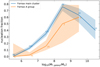 |
Fig. 5. Nucleation fraction as a function of host galaxy stellar mass for the Fornax main cluster (blue) and the Fornax A group (orange). The shaded regions denote the 68% binomial confidence interval based on the Wilson score interval (Wilson 1927). For both sub-samples, a bin width of 1 dex was used and the number of galaxies per bin is labelled in the plot. Due to the low number of galaxies, we omit bins with M* > 1010 M⊙ from the Fornax A group and M* > 1011 M⊙ from the Fornax main cluster. |
Interestingly, the peak of nucleation fraction for the Fornax A group appears to be at higher galaxy masses than in the Fornax main cluster, although the modest sample size in the bins leads to the large uncertainties. Recently, Zanatta et al. (2021) found a negative relation between the halo mass of the environment and the dwarf galaxy luminosity at a given nucleation fraction. In other words, the peak of the nucleation fraction occurs at a higher galaxy stellar mass for galaxies residing in a low halo mass environment, which corroborates our results.
At the low-mass end, as the galaxy stellar mass decreases, the nucleation fraction also drops. This feature could be due to our detection limit (visual limit at M*, nuc ≈ 104.5 M⊙), where we cannot always detect the lowest mass NSCs. On the other hand, it is possible that there is a limit to the mass of GCs that can survive the in-spiral process due to dynamical friction when forming NSCs (see e.g., Leaman & van de Ven 2021). As mentioned, upcoming surveys and data with a low enough seeing and resolution should be able to shed light on this
Clearly, the environment plays a role in the nucleation of galaxies. As such, we also consider the nucleation fraction as a function of projected cluster- and group-centric distance between the Fornax main cluster and the Fornax A group. In Fig. 6, we find the nucleation fractions peak towards the cluster centre and decrease with increasing distance, and that the nucleation fractions are generally lower in the Fornax A group than in the Fornax main cluster across bins of projected distance. This is in line with the earlier Fornax study of Venhola et al. (2019), who also estimated the 3D deprojected radial density distribution of dwarfs and found that those in the core of the Fornax main cluster are almost exclusively nucleated early-type dwarfs, with the non-nucleated dwarfs residing at further distances.
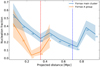 |
Fig. 6. Nucleation fraction between the Fornax main cluster (blue) and the Fornax A group (orange) as a function of projected distance (using NGC1399 and NGC1316 as the centre for the Fornax main cluster and Fornax A group, respectively). The shaded regions denote the 68% binomial confidence interval. The number of galaxies in each bin are annotated in the plot. The dashed vertical lines denote the same limits as in Fig. 1. |
Surprisingly, we find that the nucleation fractions appear to increase beyond the virial radius for both environments. In the case of the Fornax A group, the increase in the nucleation fraction towards the outskirts appears to be due to two (of three) nucleated galaxies with the furthest group-centric distances, located between the Fornax main cluster and the Fornax A group. In comparison, nucleated galaxies appear in all directions beyond the virial radius around the Fornax main cluster. If the two nucleated galaxies were instead considered as members of the Fornax main cluster, the nucleation fraction of the outermost bin for Fornax main cluster would increase from 0.3 (6 out of 20) to 0.36 (8 out of 22). At the same time, the outermost bin for the Fornax A group would decrease from 0.25 (2 out of 8) to 0 (0 out of 6). This suggests that the nucleation fraction beyond the virial radius for the Fornax A group is tenuous at best, but it appears to be real for the Fornax main cluster. Additionally, to check if the distribution is dependent on the mass of the galaxies (i.e. more massive dwarfs tend to be located towards the centre of the cluster, which could result in the peak in nucleation fraction), we limit the galaxies in Fig. 6 by their stellar masses. We find that the distributions generally retain their shape, but the nucleation fractions generally decrease with lower galaxy stellar mass limits.
Given that the increase in the nucleation fraction occurs beyond the virial radii of both environments, it is prudent to compare these galaxies to those in the field environment. Baldassare et al. (2014) found a global nucleation fraction of ∼0.26 for 109 M⊙ ≲ M∗,galaxy ≲ 1011 M⊙ early-type galaxies. Recently, Poulain et al. (2021) studied the nucleation of nearby dwarfs (10 Mpc < d< 45 Mpc, and 105.5 M⊙ < M∗,galaxy < 109 M⊙; see Habas et al. 2020) in low-to-moderate-density environments and found a global nucleation fraction of ∼0.23 (including both early- and late-types). The Local Volume (d ≲ 12 Mpc) sample of galaxies (102.5 M⊙ < M∗,galaxy < 1011.5 M⊙) studied in Hoyer et al. (2021) has a global nucleation fraction of ∼0.24. Similarly, the analysis of Carlsten et al. (2022) of Local Volume dwarfs (105.5 M⊙ < M∗,galaxy < 108.5 M⊙) determined a global nucleation fraction of 0.23. Overall, studies in the literature find the nucleation fraction in the field to be around 0.23–0.26, which is comparable to the nucleation fractions we find beyond the virial radius, within their uncertainties.
4. Photometric properties
Here we present properties of the nuclei and their host galaxies. We also compare the properties of nucleated galaxies with non-nucleated galaxies in our sample. Given that our sample of nucleated galaxies are overwhelmingly early types, this can lead to many differences between the host properties to be due to the early or late type rather than nucleation. Therefore, we compared the quantities of nucleated and non-nucleated galaxies for early types only. We present some of the derived properties of the nuclei in Table 2 for a few galaxies as examples; the full table with our whole sample can be found at the CDS.
Photometric properties of our nuclei from early-type hosts.
4.1. Colours
Based on multi-component decompositions, we used the magnitudes from the nucleus component to derive their integrated colours (see Sect. 2.1). In Fig. 7, we show the g′−r′ and g′−i′ colours of the nuclei in the early-type galaxies in our sample. For two of the galaxies we identified as hosting faint nuclei in Sect. 2.3, FDS12_0367 and FDS15_0232, their Sérsic+PSF decompositions fail to fit the nuclei (i.e. the PSF magnitudes reach the limiting 35 mag) in the g′ and i′ bands, respectively. As such, we exclude the corresponding galaxies from figures that show the nucleus colours. From Fig. 7, it is clear that the scatter in nucleus colours is large across a range of host galaxy stellar masses. In Fig. 8, we show that the scatter in nucleus g′−r′ colour is a function of the nucleus contrast (see Eq. (B.1)), where low-contrast nuclei tend to have higher scatter5. To reduce the scatter in colour from low-contrast nuclei, we limit the bulk of the colour analysis to nuclei with nucleus contrasts > 1 (solid points in Fig. 7). In Appendix D, we estimate the uncertainties in the nucleus colours due to the PSF model used in the decompositions. Overall, the nuclei colours are rather similar across for host galaxies with M* < 109 M⊙, with a weak or marginal increase in average colour at higher masses.
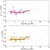 |
Fig. 7. g′−r′ (upper) and g′−i′ (lower) as a function of host galaxy stellar mass. Filled circles are galaxies with nucleus contrast > 1, whereas open circles denote those with nucleus contrast < 1. The marker size denotes the nucleus contrast (see Eq. (B.1)), with bigger points denoting higher nucleus contrast. The solid lines denote the moving (median) averages of the solid points, which were calculated using a bin width of 2 dex, and moved in steps of 0.2 dex. The shaded regions denote the corresponding standard error of the mean (SEM) in the moving averages. Nuclei with values beyond the axis limits are denoted as triangles along the x-axes. The individual error bars were estimated in Appendix D. |
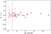 |
Fig. 8. Nucleus g′−r′ colour as a function of nucleus contrast (see Eq. (B.1)) for nuclei of early-type galaxies. The marker size denotes the nucleus contrast. The dotted vertical line denotes the limit of nucleus contrast = 1, which loosely separates nuclei with high and low scatter in colour. |
In Fig. 9, we show the difference in g′−r′ and g′−i′ colours between the nucleus component and the host galaxy for the nucleated early-type galaxies with nucleus contrasts > 1 in our sample. On the whole, there is a scatter of about zero, suggesting more or less similar colours between the nucleus and the host galaxies. The moving averages in g′−r′ and g′−i′ appear to support somewhat bluer (≲0.1 mag) nuclei for 107 M⊙ ≲ M* ≲ 108 M⊙ host galaxies.
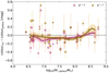 |
Fig. 9. Difference in colour between nucleus and its host galaxy as a function of the host galaxy stellar mass. We show both g′−r′ (pink) and g′−i′ (gold) colours based on the multi-component decomposition models. The moving averages were calculated using a bin width of 2 dex and moved in steps of 0.2 dex. The shaded regions denote the SEM. The marker size denotes the nucleus contrast. The uncertainties were estimated by propagating the nuclei colour uncertainties (see Appendix D) and the galaxy colour uncertainties calculated in Su et al. (2021; see their Table 1). |
Aside from the host stellar mass, we also investigate the difference in colour with projected distance. Given that the Fornax A group has a lack of nucleated galaxies, we only focused on the Fornax main cluster. From the moving averages of Fig. 10, we find that the nuclei of galaxies residing within the inner (∼0.1 Mpc) region of the Fornax main cluster appear to be marginally redder than their host galaxy, whereas the median values appear to suggest bluer nuclei at higher projected cluster-centric distances. We checked the stellar masses of the galaxies in the inner 0.1 Mpc region and found a mix of values, which suggests that the redder colour in the inner region is not due to the most massive galaxies, which have redder colours.
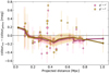 |
Fig. 10. Similar to Fig. 7, but showing the difference in colour between the nucleus and its host galaxy as a function of the projected distance. The marker size denotes the nucleus contrast. Unlike Fig. 7, here we only show galaxies in the Fornax main cluster. |
4.2. Stellar mass
To estimate the mass of the nuclei we tested two methods: going through the nucleus to host galaxy flux fraction in the r′ band only (and multiplying by the host galaxy stellar mass), and applying the g′, r′, and i′ band magnitudes of each nuclei from multi-component decompositions to Eq. (1). In Fig. 11, we show both stellar mass estimates as a function of the host galaxy’s stellar mass, which appear to be similar to each other overall. We find that the nucleus mass estimates from Eq. (1) have a larger scatter towards the low-mass end than the mass inferred from the r′ band flux fraction, although the linear fits appear to be similar. From the linear fits we obtain the following relations:

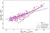 |
Fig. 11. Nucleus stellar mass as a function of the host galaxy stellar mass. We applied two estimates for the nucleus stellar mass: from r′ band nucleus flux fractions (violet) and Eq. (1) (light brown). The linear fits for both estimates are shown as solid lines. For comparison, we also include the relations from Neumayer et al. (2020; their Eq. (1)) and Georgiev et al. (2016; their early-type sample) as dashed and dash-dotted black lines. The nucleus stellar mass based on Eq. (1) for FDS12_0367 and FDS15_0232 have been omitted due to too faint g′ and i′ band nucleus magnitudes. |
for the Eq. (1) nucleus stellar mass, and

for stellar mass based on r′ band flux fractions. Comparing Eq. (6) to that of Neumayer et al. (2020; their Eq. (1)), we see that our relation has a steeper gradient ( against
  ), despite covering a comparable stellar mass range (106 M⊙ ≲ M*, galaxy ≲ 1011 M⊙). The largest difference occurs at the highest mass end, where we have much more massive nuclei than their relation predicts. Conversely, the relation from Georgiev et al. (2016) for early-type host galaxies (108 M⊙ ≲ M*, galaxy ≲ 1011 M⊙) has a steeper gradient (i.e.
  ) than our relation, which fits with our massive galaxies but clearly deviates for low-mass galaxies. As is evident in Fig. 11, the log nucleus stellar mass relation is not linear with log galaxy stellar mass, which can lead to varying gradients depending on the sample. Using two linear fits with a split at M*, galaxy = 108.5 M⊙ for nucleus stellar masses based on the r′ band flux fraction, we find that
for the lower mass galaxies, and

for the higher mass galaxies in our sample.
The deviation from linearity in nucleus stellar mass can be seen more clearly when we consider the nucleus flux fraction as a function of host stellar mass (see Fig. 12). Here, we estimate the nucleus flux fraction based on the multi-component decomposition models in the r′ band. From the moving average, we find that the nuclei with host masses of M* ≲ 109 M⊙ clearly follow a trend where the nucleus flux fraction decreases with increasing host mass. However, the trend changes for galaxies with M* ≳ 108.5 M⊙, reaching a minimum at fnuc/ftotal ∼ 0.005 and roughly plateauing with increasing host stellar mass. This feature for high-mass galaxies is reminiscent of what was observed in Sánchez-Janssen et al. (2019a), that is, an ‘uptick’ in the ratio of nucleus and host stellar mass (i.e. the nucleus mass fraction) for M* ≳ 109.5 M⊙. Interestingly, Neumayer et al. (2020) found a ’bump’ instead of an uptick, in that the nucleus mass fraction increases around 109.5 M⊙ but decreases again with increasing galaxy stellar mass (see their Fig. 12). They attributed this difference to the inclusion of galaxies from Lauer et al. (2005) in their sample. Despite the difference at the high-mass end, from Fig. 12 we find that the moving average at lower galaxy masses (M* ≲ 108 M⊙) coincides with the Neumayer et al. (2020) relation except being lower by a factor of 0.2 dex, as both have an approximate  dependence.
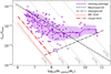 |
Fig. 12. Nucleus flux fraction as a function of host galaxy stellar mass for all nucleated early-type galaxies. The moving average (violet) was calculated using a bin width of 2 dex, and moved in steps of 0.2 dex (based on log10(fnuc/ftotal) instead). The shaded region denotes the 1σ uncertainty within the moving average bins. The dashed and dot-dashed black lines denote the relation from Neumayer et al. (2020; their Eq. (1)) and Georgiev et al. (2016; their early-type sample), respectively. The dotted and dot-dashed red lines denote the estimated detection limits based on BIC and visual inspection, respectively. The dotted grey lines denote constant nucleus stellar masses. |
4.3. Nucleated versus non-nucleated
Given that nucleation is dependent on the host galaxy property (i.e. their stellar mass; see Fig 5), we investigated whether the structural properties of galaxies also differ with nucleation. We used a combination of quantities derived from the Sérsic component of Sérsic+PSF decompositions (g′−r′, Re, n, and  ) as well as non-parametric morphological indices (C, A, S, G, M20, and Δ(g′−r′)) to measure the global properties of the host galaxies. We chose these quantities since they allow for a more homogeneous treatment of our galaxies, as opposed to directly comparing the internal structures such as bulges or bars, which are not present in all galaxies. The quantities were defined in detail in Su et al. (2021), so here we only provide a brief summary. The g′−r′ colour was calculated based on the total magnitudes from the decomposition models. The Re and n, and
  were based on the r′ band decompositions. The concentration (C), asymmetry (A), and clumpiness (S) indices quantify the central concentration, rotational asymmetry, and the amount of small sub-structures in a galaxy. The Gini coefficient (G) denotes the (in)equality in the distribution of flux across a galaxy, whereas the second order moment of the brightest 20% of flux (M20) indicates the variance in the brightest parts of a galaxy. Finally, Δ(g′−r′) is the difference in colour between the outer (1Re to 2Re) minus inner (0 to 0.5Re) region of a galaxy; so, a positive Δ(g′−r′) implies a bluer inner region than its outskirts. The non-parametric quantities were calculated including the nucleus, such that we would expect C to be higher for nucleated galaxies.
Previous studies have noted the differences in the stellar masses and structures between nucleated and non-nucleated early-type galaxies (e.g., Eigenthaler et al. 2018; Venhola et al. 2019; Sánchez-Janssen et al. 2019a; Poulain et al. 2021). However, given the clear dependence between structural quantities and the galaxy stellar mass (see the first column of Fig. 13), and the difference in the stellar mass distributions between nucleated and non-nucleated galaxies (see Fig. 3), it is not clear how much the differences in structural quantities can be attributed to the stellar mass and how much to nucleation. Hence, following Su et al. (2021), we removed the mass dependence for each quantity by subtracting the moving averages from the measured values, which we refer to as the residual quantities. This allows us to compare the difference between the two sub-samples across the range of stellar mass (see Col. (2) of Fig. 13).
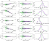 |
Fig. 13. Structural quantities of the nucleated (violet) and non-nucleated (green) early-type galaxies in the Fornax main cluster and Fornax A group. Column (1): structural quantities as functions of the galaxy stellar mass. The black lines denote the moving averages (median). Column (2): residual quantities, calculated as the measured quantities minus moving average from Col. (1). The solid lines denote the moving averages of the residual quantities. The dashed grey vertical lines denote the range where both samples overlap in stellar mass. Column (3): histograms of the residual quantities between nucleated and non-nucleated galaxies within the overlapping stellar mass range. The coloured dotted lines denote the median value of each sub-sample. For brevity, here we show quantities of interest. The full plot with all considered quantities can be found in Appendix E. |
To test whether the differences in the distributions of residual quantities between the two sub-samples (if any) are significant, we calculated the (two sample) test statistics of the Kolmogorov-Smirnov (KS) test, the Anderson-Darling (AD) test, the Lepage (LP) test, and the Cucconi (CU) test, under the null hypothesis that the two sub-samples are drawn from the same distribution6. We chose these four test statistics as they are non-parametric, meaning they do not make any explicit assumption that the data follows a certain distribution; and sensitive to different characteristics of a distribution, and so they provide independent ways of assessing the differences between the sub-samples. Compared to the KS test, the AD test statistic is more sensitive to the tails of the cumulative distributions rather than the centres. The LP and CU statistics test the location and scale (analogous to the mean and standard deviation, respectively, for a Gaussian distribution) of the two samples and compare their differences. As a result, all four test statistics are sensitive to a difference in the averages, dispersion, and indeed both, between the two samples. For the null hypotheses, we utilised a nominal significance level of α = 0.05 such that they can be rejected for p values less than α. In Table 3, we give the p values based on the residual quantities for nucleated and non-nucleated early-type galaxies with overlapping stellar masses (i.e. 106.4 M⊙ < M* < 1010.7 M⊙; Col. (3) of Fig. 13).
p values from hypothesis testing for residual galaxy properties.
Regarding the early-type galaxies, we find that the nucleated hosts tend to be redder in g′−r′ colour, less asymmetric, and exhibit redder outskirts relatively to their own inner regions compared to their non-nucleated counterparts at a given stellar mass. In the case of M20, the significant difference between nucleated and non-nucleated galaxies is likely due to the higher scatter rather than any difference in the mean. The redder g′−r′ colour suggests that nucleated galaxies generally have more evolved stellar populations. Additionally, the larger colour difference between the inner and outer regions (i.e. higher Δ(g′−r′)) for nucleated galaxies can be interpreted as stronger signs of ram pressure stripping (RPS), which affect a galaxy’s outskirts first (see e.g., Vollmer 2009). Finally, the nucleated galaxies are, on average, less asymmetric, which suggests that non-nucleated galaxies are potentially more susceptible to disruptions and interactions. It is possible that the difference in the host properties between nucleated and non-nucleated galaxies could be tied to the higher nucleation fraction towards the centre of the cluster or group. We explore the dependence of nucleation on the environment of the host galaxy in Sect. 6.2.
From Col. (2) of Fig. 13, there appears to be a change in the moving averages below and above M* ∼ 108.5 M⊙ for  , A, and Δ(g′−r′). Restricting the stellar mass range to M* < 108.5 M⊙, we find significant differences for the KS test (p = 0.047) and the AD test (p = 0.044) for residual
  . Moreover, we find that the moving averages differ the most at the low-mass end. This difference could be due to a bias in the detection of nuclei, where nucleated galaxies with low surface brightness would have a higher nucleus contrast than their high surface-brightness counterparts. For A and Δ(g′−r′), we found that all test statistics remain significant: pKS = 0.009, pAD = 0.006, pLP = 0.006, pCU = 0.005 for residual A, and pKS = 0.021, pAD = 0.009, pLP = 0.029, pCU = 0.028 for residual Δ(g′−r′).
Recent studies have found that nucleated cluster dwarfs tend to have higher axial ratios (q) than their non-nucleated counterparts (Lisker et al. 2007; Eigenthaler et al. 2018; Venhola et al. 2019; Sánchez-Janssen et al. 2019b; Poulain et al. 2021). Furthermore, by modelling the dwarfs as triaxial ellipsoids, Sánchez-Janssen et al. (2019b) inferred that the nucleated dwarfs from the cores of the Virgo and Fornax clusters have higher intrinsic (vertical) thickness than the non-nucleated galaxies. Here, we address this difference between nucleated and non-nucleated galaxies with our sample, also considering the surface brightness of our dwarfs with 106.2 M⊙ ≲ M*, galaxy ≲ 107.8 M⊙7 (equivalent to the limits set in Sánchez-Janssen et al. 2019b).
In Fig. 14, we show the residual  as a function of the axial ratio for galaxies within the stellar mass range, as well as their distributions as histograms in the sub-plots. We confirm that our nucleated galaxies tend to have higher axial ratios, with the peak of the distribution around 0.85. Comparatively, we do not find a clear peak for the non-nucleated galaxies, with the majority spanning from 0.5 to 0.9, and the maximum occurring around 0.75. We do not find two peaks for the nucleated sample as Sánchez-Janssen et al. (2019b) reported, although this may be due to the differences in our sample (i.e. their sample consists of galaxies from both the cores of the Virgo (< 300 kpc) and Fornax (< 350 kpc) clusters). In comparison, our axial ratio distributions are similar to the Virgo dwarfs of Lisker et al. (2007; see their Fig. 3), which showed a peak at an axial ratio of 0.9 for the nucleated galaxies and a flatter plateau of axial ratios between approximately 0.5 and 0.8.
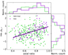 |
Fig. 14. Residual |


Intriguingly, using Spearman’s rank correlation coefficient (rs), we find a significant positive correlation between  and the axial ratio for the nucleated galaxies (rs = 0.53, p value ≪ 0.001)8 but not for the non-nucleated galaxies (rs = 0.09, p value = 0.16). Substituting q = 0.5 into the linear relation and extrapolating to q = 1, we would expect a nucleated galaxy to experience a change in (residual)
  of 1.18 ± 0.24 mag arcsec−2, or a factor of approximately 2.4–3.6 brighter. This is of the same order as the factor of ∼2 that we would expect from oblate spheroids (when viewed from different orientations). Conversely, the lack of correlation for the non-nucleated galaxies suggests that they are likely better described as triaxial ellipsoids (such as in Lisker et al. 2007; Sánchez-Janssen et al. 2019b). Splitting the sub-sample of nucleated and non-nucleated at M*, galaxy = 107 M⊙ (equivalent to Mg′ = −12.5, as used in Sánchez-Janssen et al. 2019b), we find that the least massive non-nucleated galaxies are responsible for the lack of a significant correlation. Indeed, we find significant correlations for both nucleated and non-nucleated galaxies for 107 M⊙ < M*, galaxy < 108.5 M⊙. The trend between surface brightness and axial ratio is investigated in detail in Venhola et al. (2022).
5. Automatic model selection
The process of conducting multi-component decompositions under human supervision can be rather time-consuming, particularly in identifying morphological structures in the galaxies and considering the type of model which best fit them. Hence, while multi-component models exist for our galaxy sample, there is merit in developing methods that can provide insight into the structures of galaxies in an unsupervised manner. Here, we focused on the nucleation of early-type galaxies, and specifically whether a galaxy hosts a central nucleus. To do so, we used the single Sérsic and Sérsic+PSF decomposition models (conducted in the r′ band) to test the model selection criteria. These two models were chosen due to the general versatility of the Sérsic function in fitting galaxy light profiles, whilst the PSF models fit the nuclei of our galaxies well without many free parameters, due to them being unresolved in our images. Most importantly, both models are simple and can produce reasonable fits to a variety of galaxies with rudimentary initial values, which is desirable for an unsupervised methodology. In this section, we test both formulations of the BIC used in Sect. 2.2 as the model selection criteria.
In Fig. 15, we show the nucleus flux fraction (in this case the total PSF flux divided by total Sérsic and PSF flux from Sérsic+PSF models) as a function of the galaxy stellar mass. Galaxies with fnuc/ftotal < 10−4 are shown as triangles along the x-axis, as their PSF components have reached the 35 mag limit without excess central flux above the Sérsic component. A few galaxies that we identified as nucleated appear in this region due to their high central concentration from morphological structures (e.g., bulges, bars, barlens). Given that these galaxies are massive (M* > 109 M⊙), the nuclei represent a much smaller fraction of the galaxy light and are easily dominated by the Sérsic component. Nevertheless, we find the general shape of the nucleated galaxies in Fig. 15 to be very similar to that of Fig. B.2, where the former is based on Sérsic+PSF models and the latter is based on multi-component models. This similarity demonstrates the general robustness of our nucleus flux estimates, as on the whole they do not appear to heavily depend on the applied decomposition model (with only a few high-mass exceptions).
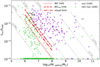 |
Fig. 15. Nucleus flux fraction as a function of host stellar mass, based on Sérsic+PSF models. Nucleated galaxies are shown in violet and non-nucleated galaxies are shown in green. Those with a fitted nucleus total magnitude of 35 mag are shown as triangles along the x-axis. The dotted, dot-dashed, and dashed red lines are the estimated BIC, visual, and BICres detection limits, respectively, based on our synthetic nucleation tests (see Sect. B.1). |
To test the performance of classifying nucleated and non-nucleated galaxies, we applied both BIC and BICres to our sample of galaxies9. Here, the BIC classifies a galaxy as nucleated if ΔBIC = BICSérsic−BICSérsic+PSF > 0 (i.e. a Sérsic+PSF model is preferred over a single Sérsic model). The BIC and BICres classifications were then compared to our nucleated and non-nucleated labels. To evaluate the accuracy of the classifications, we assigned each galaxy with one of four labels: true positive, true negative, false positive, and false negative. True and false denote whether the galaxies were correctly or incorrectly classified based on the labels, whereas positive and negative denote nucleated and non-nucleated, respectively. From Fig. 16 and Table 4, we find that both BICs generally have a low number of incorrect classifications (i.e. false positives and false negatives). For all galaxies in our sample, we find an overall accuracy of 89% and 93% for BIC and BICres, respectively. However, given that many of the higher mass galaxies tend to have multiple components (e.g., bulge, bar), we also excluded galaxies with M* > 109 M⊙ and found that the accuracies improved slightly for both BIC and BICres (93% and 97%, respectively).
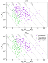 |
Fig. 16. Accuracy of BIC (upper) and BICres (lower) in classifying nucleated and non-nucleated early-type galaxies. True (i.e. correct) and false (i.e. incorrect) classifications are denoted by circles and crosses, respectively. Galaxies where GALFIT fails to find a nucleus (i.e. the triangles from Fig. 15) have been omitted. The BIC classification accuracies are shown in Table 4. |
From Table 4, we find the BIC is able to correctly identify more nucleated galaxies (true positives), but also misidentify more non-nucleated galaxies as nucleated (false positives). This, along with the lack of misclassified nucleated galaxies (false negatives), provides evidence of the sensitivity of the BIC to perturbations at the centre of the galaxies10. This is also supported by the lower nucleus detection limit for the BIC than for the BICres (Fig. 16). In the case of BICres, there are much fewer false positives at the expense of more false negatives. Nonetheless, the total number of misclassified galaxies are lower for BICres, hence its higher overall accuracy.
Classification accuracies for BIC and BICres.
In terms of the false positives (i.e. ΔBIC > 0 but non-nucleated), for M*, galaxy < 109 M⊙ we find a significant overlap (37 out of 39) with the false positives identified in Sect. 2.3, which were based on multi-component models. From inspection of the residual images, we confirm that these false positives can also be classified by the two types of false positives for the same reasons. Whilst it is unlikely, we do not entirely disregard the possibility that some of the low-mass false positives could actually host a nucleus. Future works could shed light on this, as currently there are no images with the required spatial resolution available.
6. Discussions
We find that the nucleation of Fornax galaxies is dependent on a number of factors, such as the galaxy stellar mass and the environment that they reside in. In this section, we discuss the nature of the nuclei themselves, their formation mechanisms, and the role that the environment plays in nucleation.
6.1. Growth of NSCs
A prevailing mechanism of NSC growth is the infall of GCs to the minimum of the potential of a galaxy due to dynamical friction (Tremaine et al. 1975). Recently, Gnedin et al. (2014) modelled the evolution of GCs in galaxies and found that not only can the NSCs form rather quickly (≲1 Gyr), but also that their mass correlates with the host galaxy mass:  (from their Eq. (13)). The exponent of 0.5 is consistent with our moving average from Fig. 12 for galaxies with M*, galaxy ≲ 108.5 M⊙, as well as with the exponent of 0.48 from Neumayer et al. (2020). However, the models of Gnedin et al. (2014) were based on much more massive galaxies (M*, galaxy > 1010 M⊙), and the extrapolation of their scaling relation leads to much too massive NSCs at lower galaxy stellar masses. On the other hand, the model of Antonini et al. (2015) finds that GC in-spiral alone is insufficient to reproduce the observed NSC stellar masses at high galaxy stellar masses. However, assuming a linear extrapolation, the model qualitatively appears to be in line with our moving average of fnuc/ftotal with galaxy stellar mass (see Fig. 17). It is therefore possible that the low-mass nucleated galaxies in our sample could have grown a significant portion of their nuclei via the in-spiral of GCs.
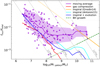 |
Fig. 17. Comparison of different NSC formation mechanisms with our nucleated early-type galaxies. The violet points, solid line, and shaded region denote our nucleated galaxies (same as in Fig. 12). We consider the maximum NSC mass via tidal compression of gas (i.e. an upper limit; red; Emsellem & van de Ven 2008), GC in-spiral (orange and cyan; Gnedin et al. 2014 and Antonini et al. 2015, respectively), and a combination of GC in-spiral and galaxy evolution models (blue; Antonini et al. 2015). The black hole scaling relation (green; Greene et al. 2020) is included to illustrate the evolution of black holes. The dotted portion of the coloured lines denote an extrapolation of the original relation. The dotted grey lines denote constant nucleus stellar masses. |
An additional mechanism is the compression of gas in the central region of galaxies due to their local tidal field. In particular, Emsellem & van de Ven (2008) found that the radial tidal forces are naturally compressive in the central regions of galaxies with relatively shallow central density (i.e. Sérsic index n ≲ 3.5). Furthermore, they found the relation log10(M+/M*, galaxy)∼ − 1.9 × n − 0.4, where M+ is the limiting mass of the NSC, above which the tidal forces become disruptive. Applying this relation to our nucleated galaxies, we find that only ∼22% of nuclei have masses below their M+. Moreover, we find that those with nuclei masses below their M+ have M*, galaxy ≲ 109 M⊙. This suggests that only a fraction of the nuclei could have grown purely based on tidal compression. A potential factor for this is the necessity of gas, which many of our galaxies lack in the present day. Nevertheless, we do not rule out the possibility that these galaxies were gas-rich in the past and formed NSCs at an earlier epoch. Based on spectroscopic studies of NSCs from Johnston et al. (2020) and Fahrion et al. (2021), there is evidence to suggest that the star formation histories of the NSCs not only vary from their host galaxies, but some even exhibit multiple episodes of star formation. This suggests that in situ star formation also plays an important role in the growth of the NSCs, particularly for massive (M* > 109 M⊙) galaxies (see also Neumayer et al. 2020).
In Fig. 17, we overlay the various mechanisms discussed on top of our nucleated sample. We also include the model from Antonini et al. (2015), which combined both mechanisms of GC infall and in situ star formation as well as the effects of central black holes on NSC growth. In particular, they found that the central black holes can inhibit NSC growth for massive (M* > 1010 M⊙) galaxies. Recently, the N-body simulations of Askar et al. (2021) show that the merging of star clusters can potentially form black holes that grow via gas accretion to become supermassive black holes. Based on early-type galaxies, Greene et al. (2020) found a trend of log10(MBH) = (1.33 ± 0.12)×log10(M*, galaxy/(3 × 1010 M⊙)) + (7.89 ± 0.09) (from their supplement Table 5). The gradient of this log–log relation is steeper than the gradient we find in Eq. (8) for our massive galaxies, which suggests that the central black holes grow faster than NSCs. This difference in gradient could be interpreted as a sign of the disruptive effects of central black holes on NSC growth.
6.2. Dependence on the environment
6.2.1. Nucleation fraction
From Sect. 3, we find that the nucleation fraction depends on the galaxy environment, with most nucleated galaxies found at the centre of the Fornax main cluster and Fornax A group. Furthermore, we find the overall nucleation fraction of the Fornax main cluster to be higher than in the Fornax A group. This difference in nucleation fraction between environments is in line with the findings of Sánchez-Janssen et al. (2019a) and Carlsten et al. (2021), who found similar nucleation fractions in the Virgo and Fornax clusters, whereas the Coma cluster and the Local Volume had higher and lower nucleation fractions than the Fornax cluster, respectively. Similarly, Zanatta et al. (2021) found a trend between the halo mass of the environment and the galaxy luminosity at a given nucleation fraction (their Fig. 7). In contrast, Baldassare et al. (2014) found similar nucleation fractions between Virgo cluster galaxies and galaxies in the field. As Neumayer et al. (2020) discusses, this apparent discrepancy could be due to the difference in the stellar mass of the samples (Baldassare et al. 2014 sampled high-mass galaxies, whereas Sánchez-Janssen et al. 2019a mainly sampled low-mass galaxies). According to Poulain et al. (2021), their field dwarfs have lower nucleation fractions than dwarfs from the core of the Virgo cluster11. Based on our sample of dwarf and massive galaxies, we find that the nucleation fraction for galaxies beyond the virial radius of the Fornax main cluster (and to some degree, the Fornax A group) is comparable to the nucleation fraction of galaxies in the field (see Sect. 3).
Recently, Leaman & van de Ven (2021) studied the link between the nucleation fraction of galaxies and the environment that they reside in. In particular, they focused on the GC in-spiral mechanism and defined a limiting GC mass above which they can survive mass loss during in-spiral, and hence contribute to the NSCs. Based on their model, they found that the observed shape of nucleation fraction as a function of galaxy mass (e.g., Fig. 5), and the location of the peak, can be reproduced depending on the assumed galaxy size–mass scaling relation and the GC mass function. Furthermore, they argue that the observed differences in nucleation fractions in different halo mass environments (e.g., in Sánchez-Janssen et al. 2019a; Zanatta et al. 2021) are likely due to the preferential disruption of the most diffuse (low surface brightness) galaxies by the cluster potential, which also tend to be low mass and non-nucleated. In this scenario, over time, those that survive the disruption are generally the more massive, higher surface brightness galaxies, which have relatively higher nucleation fractions. This can lead to two features in the observed nucleation fractions: the correlation between cluster mass and nucleation fraction at a given galaxy mass (e.g., Zanatta et al. 2021), as the strength of tidal disruption is correlated with the cluster mass; and the high nucleation fraction at the cluster centre, since the stronger tidal effects at the cluster centre would be more efficient in disrupting the galaxies.
An important caveat to this scenario is the ’initial’ galaxy size–mass relation (i.e. the population of galaxies in the cluster before they are affected by the cluster potential), specifically for galaxies at the low-mass end (e.g., M* < 107 M⊙). Leaman & van de Ven (2021) adopted a size–mass relation with an inflexion at ∼109 M⊙, such that, on average, galaxies below and above this mass tend to have larger sizes. Although we recognise that our observed size–mass relation is of the present day, and hence can differ from the size–mass relation of the past (in other words, the ’initial’ galaxy size–mass relation), we do not find any signs that point to such a feature in our moving average (see Col. (1) of Fig. E.1). For such a change in the size–mass relation, this would imply that the tidal effects must be very efficient to leave no trace of these very diffuse galaxies. Recently, Marleau et al. (2021) studied ultra-diffuse galaxies (UDGs) in low-density environments (as a part of MATLAS). They defined UDGs as those with Re ≥ 1.5 kpc and a central surface brightness of μ0, g ≥ 24 mag arcsec2. From inspection, their sample generally appears to be in-line with our size–mass scaling relation, and they found roughly comparable nucleation fractions to our FDS sample (20 out of 59 = 0.34 and 148 out of 557 = 0.27, respectively). Given that the sample from Marleau et al. (2021) resides in low-density environments, we do not expect the environment to be able to efficiently disrupt UDGs. As such, some of the faint, low-mass UDGs (which would appear as an upturn in the size–mass relation) should survive to the present day and be observable, and so their absence from the sample of Marleau et al. (2021) is intriguing. On the other hand, an argument could be made that these UDGs may be fainter than the detection limits from current surveys.
It is possible that in the early Universe, GCs are more likely to form in dense environments. This naturally makes galaxies residing in the core of clusters ideal candidates to host more GCs, which over time can transform into NSCs via dynamical friction. Lisker et al. (2013) showed that early-type galaxies have typically resided in clusters for several Gyr, and Sánchez-Janssen & Aguerri (2012) found that the properties of early-type galaxies in Virgo are not consistent with recent environmental transformations. Overall, in order to address the effects of tidal disruption in a more quantitative manner, simulations that model the cluster potential and account for the galaxy mass distribution, including the lowest mass dwarfs, are required.
6.2.2. Galaxy structures
Given the apparent dependence of nucleation on projected distance, and the difference in galaxy properties between nucleated and non-nucleated galaxies (see Fig. 13), we also test whether environmental mechanisms (e.g., RPS, tidal interactions) could play a role in the observed differences in the structural quantities. Since the majority of our nucleated galaxies are from the Fornax main cluster, Fig. 18 shows the galaxy properties of early-type Fornax main cluster galaxies (with overlapping stellar mass between nucleated and non-nucleated sub-samples) as a function of projected distance. Logically, one could argue that if the galaxies reside in the same environment, the environmental effects should apply to both nucleated and non-nucleated galaxies, and we should not expect any differences between the two sub-samples. However, it is not implausible that nucleated galaxies may have experienced more (or fewer) environmental effects in their past that lead to nucleation, or vice versa for non-nucleated galaxies. This can occur as the efficiencies of the environmental mechanisms can vary depending on the orbital parameters of the galaxies falling into the cluster (e.g., Smith et al. 2015; Bialas et al. 2015). Alternatively, the conditions in high-density regions in the past could have been more favourable towards NSC formation (or the formation of GCs that then spiral towards the galaxy centre), which can lead to the observed higher nucleation fraction towards the cluster centre, and hence experience environmental effects for a longer period. In such cases, we might expect a difference in the projected distance trends between nucleated and non-nucleated galaxies.
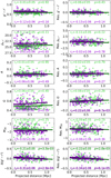 |
Fig. 18. Structural quantities of nucleated (violet) and non-nucleated (green) early-type galaxies in the Fornax main cluster only, as a function of the projected distance. Only galaxies with overlapping stellar mass are shown (i.e. Col. (4) from Fig. 13). The measured (left) and residual (i.e. mass-trend corrected; right) quantities are shown. The solid lines are based on linear fits to the data and are only meant as visual guides to the Spearman’s rank correlation coefficient, rs. For each quantity, the rs and associated p values are annotated in the corresponding sub-plots. |
To test whether there are any significant differences in the projected distance trends between nucleated and non-nucleated galaxies, we calculated the Spearman’s rank correlation coefficient rs and the associated p value12 for each galaxy quantity. From Fig. 18, we find that the quantities (g′−r′, Re,  , A) that had significantly different distributions between nucleated and non-nucleated galaxies do not have significant projected distance trends. If we interpret the projected distance as a rough indicator of the time spent for environmental mechanisms to act within the cluster (as Su et al. 2021 did), this implies that the environmental mechanisms are unlikely to be the main driver in the observed differences in these galaxy quantities.
Of all the structural quantities tested, we only find significant trends for the residual Gini coefficient (G) and the outer-to-inner colour difference (Δ(g′−r′); see Fig. 18) as a function of projected cluster-centric distance. In the case of Δ(g′−r′), both nucleated and non-nucleated galaxies show significant trends. The negative values of rs suggest that galaxies towards the centre of the cluster have bluer inner regions than those in the cluster outskirts. Su et al. (2021) interpreted this as a result of RPS acting outside-in. Given the clear cluster-centric trends for both nucleated and non-nucleated galaxies, this suggests that the RPS affects both types of galaxies equally. However, for G we find a significant trend for nucleated galaxies, but not for non-nucleated galaxies. The positive rs suggests that nucleated galaxies closer to the cluster centre have a more homogeneous distribution of light (i.e. the galaxy light is more evenly distributed amongst the pixels). Overall, the general absence of difference in the cluster-centric trends (or lack thereof) between the nucleated and non-nucleated galaxies suggests that the environmental effects affect both types of galaxies to a similar extent, on average. Furthermore, the lack of cluster-centric trends with the structural quantities suggests that environmental mechanisms are unlikely to be directly responsible for the observed differences between the nucleated and non-nucleated galaxies (see Fig. 13). Nevertheless, the environment clearly plays an important role in the nucleation of galaxies in Fornax.
6.3. Comparison to UCDs
Ultra-compact dwarfs (Hilker et al. 1999; Phillipps et al. 2001) are compact objects with typical half-light sizes of < 100 pc and stellar masses of ≳106 M⊙ (e.g., Drinkwater et al. 2003; Evstigneeva et al. 2007; Mieske et al. 2008). They appear to be ubiquitous, having been observed in both clusters and in lower density environments (see Liu et al. 2020 and references therein). UCDs appear quite similar to the brightest, most massive GCs in the GC luminosity functions of galaxies, as well as resembling isolated NSCs without a visible host galaxy. As such, the formation channels for UCDs are thought to follow two mechanisms: the stripping of NSCs from nucleated galaxies via mergers or tidal disruption (Bekki et al. 2003; Goerdt et al. 2008; Pfeffer & Baumgardt 2013; Norris et al. 2015; Janz et al. 2016), or the coalescence of massive stellar clusters, which form the most massive GCs (Fellhauer & Kroupa 2002).
Here, we would like to compare the observed properties of UCDs in Fornax with the nuclei from our sample. For our UCD sample, we compiled the likely UCD candidates based on photometry in Saifollahi et al. (2021) and the catalogue of spectroscopically confirmed Fornax compact objects (including GCs and UCDs) from Wittmann et al. (2016). The UCD candidates in Saifollahi et al. (2021) were selected based on a limit of mg′ < 21 mag (Mg′ = −10.5 mag), as well as a combination of colours spanning the visible wavelengths to near infrared. To ensure a homogeneous sample, we applied the same mg′ magnitude cut for the Wittmann et al. (2016) sample to select the UCDs13. This resulted in 44 + 65 = 109 UCDs from the Fornax main cluster. We estimated the stellar mass of UCDs based on their colours and Eq. (1) and used the nucleus stellar masses based on r′ band flux fractions.
In Fig. 19, we compare the g′−r′ colour of the nuclei and UCDs as a function of their stellar masses. As in Sect. 4.1, here we select nuclei with nucleus contrast > 1 for the colour comparisons. For reference, we also include the master GC catalogue of Cantiello et al. (2020), which includes photometrically and spectroscopically confirmed GCs (see their Table 5). At first glance, the plot seems to suggest that UCDs tend to be more massive than nuclei. However, this is due to the magnitude limit from the UCD compilation sample; thus, UCDs with lower stellar masses are not well represented. In terms of the g′−r′ colours, we find that UCDs have slightly redder mean colours compared to nuclei (0.64 and 0.56 for UCDs and nuclei, respectively) and similar standard deviations in colour for UCDs and nuclei (0.14 and 0.18 for UCDs and nuclei, respectively). Considering the nuclei and UCDs within an overlapping range in stellar mass (106 M⊙ ≲ M* ≲ 107.5 M⊙), the colour distributions are rather similar (mean and standard deviation in g′−r′ are 0.65 and 0.13 for UCDs, and 0.60 and 0.13 for nuclei, respectively). This comparability in colours potentially alludes to similar stellar populations between UCDs and nuclei.
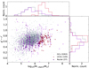 |
Fig. 19. g′−r′ colour as a function of stellar mass for GCs (grey), UCDs (crimson), and nuclei (violet). As in Fig. 7, the nuclei with nucleus contrast > 1 are shown as filled circles, whereas nuclei with nucleus contrast < 1 are shown as open circles. The upper and right panels show the stellar mass and g′−r′ distributions, respectively. The nuclei uncertainties are the same as in Fig. 7. The UCD uncertainties are generally within the size of the points, and hence they are omitted. |
Additionally, we compare the projected distance distributions of the nuclei and UCDs. In Fig. 20, we show the nuclei (regardless of nucleus contrast), UCDs, and GCs in the Fornax main cluster. Overall, a significant fraction of UCDs are located at the central (< 0.2 Mpc) region of the Fornax main cluster. Towards the cluster outskirts and beyond (> 0.5 Mpc), we do not find any particular differences between nuclei and UCDs. Applying the four test statistics (KS, AD, LP, CU), we find that the distributions of projected distances are significantly different for the two samples (p value < 0.001). To test the significance further, we split our UCD sample by M* = 106.6 M⊙ into high- and low-mass sub-samples and recalculated the hypothesis tests with respect to the nuclei. We find that both the low- and high-mass UCDs are significantly different from our nuclei. When we also restrict the nuclei sample to within the same stellar mass range to match the UCDs’ sub-samples, we find that the high-mass UCDs and nuclei remain significantly different, but not for the low-mass UCDs and nuclei (p > 0.05). This appears to be due to the prevalence of high-mass UCDs at the cluster centre, whereas the low-mass UCDs tend to be located beyond and are more evenly distributed with distance. Whilst the higher number of UCDs at the cluster centre compared to nuclei is consistent with the scenario that UCDs are the remaining nuclei from disrupted dwarf galaxies, it remains possible that some of the UCDs are, in fact, massive GCs, which are also concentrated at the centre of the cluster.
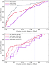 |
Fig. 20. Distribution of projected cluster-centric distance for GCs (grey), UCDs (crimson), and nuclei (violet). Here, only nuclei from early-type galaxies in the Fornax main cluster are shown. The upper panel shows the cumulative distribution of all the compact objects, respectively. The lower panel shows the cumulative distributions of the low- (dotted) and high- (dashed) mass sub-samples of UCDs split at M* = 106.6 M⊙ and the nuclei within the accompanying UCD stellar mass ranges. The dotted blue line denotes the virial radius of the Fornax main cluster. |
We also tested the scenario of UCDs as stripped nuclei with the cosmological simulations of Goerdt et al. (2008). By allowing M33-like haloes to evolve in a Virgo-like cluster for 5 Gyr, they found a set of orbital parameters (pericentre of apocentre) where the galaxies (with and without a gas disc) would be completely disrupted, leaving only the nuclei. Of course, not all galaxies become disrupted, with those that survive appearing as nucleated galaxies in the cluster. Hence, the scenario of UCDs as stripped nuclei can be tested by comparing the predicted number of UCDs and nucleated galaxies from the simulation to those observed in the cluster. We followed Goerdt et al. (2008) by determining the UCD fraction, fUCD = NUCD/(NUCD + Nnuc), as a function of projected cluster-centric distance, and comparing to the observations. As a caveat, we recognise that not all UCDs form from disrupted nucleated galaxies, with the possibility that low-mass UCDs are, in fact, massive GCs. Nevertheless, we find the comparison between the observations and simulations to be illuminating with regard to examining stripped nuclei as an UCD formation channel.
In Fig. 21, we show the UCD fractions from the Goerdt et al. (2008) simulations of galaxies with and without a gas disc. We compare their predictions with our Fornax main cluster sample, as well as using the nucleated galaxies (Ferrarese et al. 2020) and UCDs (Liu et al. 2020) from the core of the Virgo cluster from the NGVS. To ensure a reasonable comparison, we only selected nucleated galaxies and UCDs within the overlapping region of both datasets. This restricts the Virgo sample to the cluster core (≲200 kpc). We selected the Virgo nucleated galaxies as those classed as certain or possible Virgo members that are nucleated or host an offset nucleus (‘Class’ = 0 or 1 and ‘Nuc ID’ = 1 or 2; Ferrarese et al. 2020, see their Tables 4 and 5). As for the Virgo UCDs, we selected those classified as ‘probable UCDs’ (‘Class’ = 1, Liu et al. 2020, see their Table 4), and we applied the same magnitude limit from Saifollahi et al. (2021). We find that the UCD fraction peaks at the centre of the Virgo cluster and drops steeply with increasing distance. Similarly, the UCD fraction peaks at the centre of the Fornax cluster, although the decrease with distance appears shallower. The predicted UCD fractions of the galaxies without gas better match the observed UCD fractions in the Virgo core. However, neither models match well with the observed UCD fractions from the Fornax main, which warrants further investigation. Interestingly, in Fig. 21 we find a second, smaller peak around the virial radius of the Fornax main cluster, which appears to be consistent with the overdensities of UCDs identified in Saifollahi et al. (2021; see their Fig. 23).
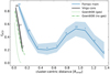 |
Fig. 21. UCD fraction (fUCD = NUCD/(NUCD + Nnuc)) as a function of projected cluster-centric distance for the Fornax (blue) and Virgo (black) clusters. We used a virial radius of 1.55 Mpc for the Virgo cluster (Ferrarese et al. 2012). The shaded regions show the 1σ binomial uncertainty. The dotted and dash-dotted green lines show the predicted UCD fractions depending on whether the UCD progenitor galaxies contain gas or not, respectively. |
7. Conclusions
In this work, we studied the properties of nucleated galaxies from the Fornax main cluster and the Fornax A group, as well as the role that the environment plays. From the Su et al. (2021) compilation of dwarfs (from FDSDC, Venhola et al. 2018) and massive galaxies (from Iodice et al. 2019; Raj et al. 2019, 2020), we selected 557 galaxies that were labelled as nucleated and non-nucleated based on visual inspection of the galaxy and residual images from multi-component decompositions. To ensure we did not miss any faint nuclei, we compiled an additional candidate list of galaxies labelled as non-nucleated from Su et al. (2021), which showed a better fit with a Sérsic+PSF model rather than a single Sérsic when using the model selection criterion BIC. This allowed us to find 20 additional galaxies that indeed hosted faint nuclei.
From our nucleation labels, we tested the accuracies of the two BIC formulations, BIC and BICres, in determining whether a single Sérsic model is preferred over a Sérsic+PSF model, and hence we were able to infer whether a galaxy was nucleated or not (Sect. 5). We investigated the nucleation fraction as a function of the galaxy stellar mass and the projected distance (i.e. distance from the centre of the environment) between the Fornax main cluster and Fornax A group (Sect. 3). We also utilised the multi-component decompositions to determine the total magnitude of the nuclei in the g′, r′, and i′ bands to determine their colours (Sect. 4.1) and stellar masses (Sect. 4.2). We also compared the structural properties of the nucleated and non-nucleated early-type galaxies through their Sérsic-derived quantities and non-parametric morphological indices (from Su et al. 2021), and we calculated the statistical significance in their differences (Sect. 4.3).
Our main results can be summarised as follows.
-
The nucleation fraction in the Fornax A group is generally lower at all galaxy stellar masses than in the Fornax main cluster, particularly regarding galaxies with M*, galaxy ∼ 107 M⊙ (see Figs. 5 and 6).
-
We find that for nucleated galaxies with 107 M⊙ ≲ M*, galaxy ≲ 109M⊙, their nuclei tend to be marginally bluer than the host galaxies themselves (see Fig. 7). More massive galaxies have redder nuclei compared to their host galaxies.
-
The relation between the nucleus and the host galaxy stellar masses follow different trends depending on the stellar mass of the galaxy. Galaxies with M*, galaxy < 108.5 M⊙ follow
 , whereas higher mass galaxies follow M∗,nuc ∝ M∗,galaxy (see Fig. 12). The relation for lower mass galaxies is consistent with the relation found in Neumayer et al. (2020), but it deviates at higher galaxy stellar masses.
 -
There are significant (p value < 0.05) differences in the distributions of residual (i.e. stellar mass-trend-removed) colour (g′−r′), asymmetry index (A), brightest second-order moment of light (M20), and outer–to–inner colour difference (Δ(g′−r′)) between nucleated and non-nucleated early-type galaxies (see Fig. 13 and Table 3).
-
For M*, galaxy ≲ 108 M⊙, we find a significant trend between residual
 and the axial ratio for the nucleated galaxies, but not for the non-nucleated galaxies (see Fig. 14). This implies that the fainter residual
  for nucleated galaxies are likely due to inclination effects, which reflect the fact that the nucleated galaxies are well described as oblate spheroids, whereas non-nucleated galaxies are better described as triaxial ellipsoids.
 -
We do not find significant correlations between the residual quantities and projected distance except for Δ(g′−r′) and G (see Fig. 18). The lack of difference in the correlations between nucleated and non-nucleated galaxies suggests that their observed differences in residual quantities are not directly due to environmental effects. Nevertheless, we do not dismiss the role of the environment, particularly on the nucleation of galaxies.
-
We find similar colours for Fornax UCDs and nuclei, in particular when considering a similar stellar mass range (see Fig. 19). Furthermore, comparing the distributions of nuclei and UCDs as functions of their projected cluster-centric distances, we find the UCDs are more concentrated towards the cluster centre than the nuclei (see Fig. 20). Additionally, we find that the UCD fraction (fUCD = NUCD/(NUCD + Nnuc)) as a function of projected cluster-centric distance peaks at the centre of the Fornax main cluster, which is consistent with the observed UCD fraction within the core of the Virgo cluster, as well as with the predicted UCD fractions from cosmological simulations of Goerdt et al. (2008) (see Fig. 21). This is consistent with the idea that UCDs may be nuclei stripped from dwarfs.
-
We demonstrate that the BIC can be used as a highly accurate method of model selection to differentiate between nucleated and non-nucleated early-type galaxies, particularly when only considering galaxies with M* < 109 M⊙ (up to 97%, see Table. 4). In principle, the scaling relations of NSCs (e.g., with NSC stellar mass and size) can be used in conjunction with the BIC to detect outliers and increase the overall detection accuracy and should be investigated in the future.
From the analyses in this work and in the literature, the big picture of NSCs (specifically, but not exclusively to Fornax) is their dependence on their host galaxies, particularly the internal and external effects they experience. The internal mechanism for NSC formation and growth is dependent on the mass of the galaxy, with different mechanisms dominating at different mass regimes (e.g., GC in-spiral and in situ star formation; see Fig. 17 and Sect. 6.1). As a result, we see that the nucleation fraction (see Fig. 5) and the NSC stellar mass (see Figs. 11 and 12) depend heavily on the host galaxy mass. On the other hand, external effects due to the cluster environment must also play a role, given that NSCs appear preferentially in high-density environments (see Fig. 6). It is not yet clear how environmental effects could lead to the high nucleation fraction at the cluster centre. Given that nucleated galaxies tend to be more massive than non-nucleated galaxies (see Fig. 3 and Sect. 6.2.1), it is plausible that non-nucleated galaxies are more susceptible to tidal disruptions, the effects of which are strongest at the cluster centre. Naturally, any nucleated galaxies that reach the cluster centre are mostly stripped of gas, and, if disrupted, can be transformed into a UCD (see Fig. 21).
In actuality, the Milky Way’s NSC is embedded within an NSD that is flatter and more extended than the NSC itself (see Launhardt et al. 2002). For reference, the NSD region (≲120 pc) contains a mass of (8 ± 2)×108 M⊙ (Nogueras-Lara et al. 2020).
In Appendix A we show the galaxy and residual images.
We used the ks_2samp and anderson_ksamp functions from the SciPy library (Virtanen et al. 2020) to calculate the KS and AD test statistics, respectively, and their corresponding p values. For the LP and CU statistics, we constructed user-defined functions in Python following Marozzi (2009).
Given the slight differences between the  moving averages between nucleated and non-nucleated galaxies (see Fig. E.1), we also tested different intervals in stellar mass where the differences were smaller (e.g., 106.7 M⊙ − 107.3 M⊙). These did not alter our results and interpretation.
Here, we evaluate the accuracy using our nucleation labels. A small caveat is that these are not strictly ground truths, which should be used instead for the true accuracy. Nevertheless, our labels provide a comparison to the accuracy from visual inspections, which has been the de facto method for detecting nuclei.
We note that the Virgo cluster may not be the most typical cluster (see Janz et al. 2021).
Wittmann et al. (2016) used a magnitude cut of mVe < 21.5 mag, where mVe denotes the ‘equivalent V’ band magnitude (see their Sect. 2.4).
Additionally, we compared our nucleation label with the Advanced Camera for Surveys Fornax Cluster Survey (ACSFCS) galaxies of Turner et al. (2012). We find that the nucleation labels agree for the majority (29 out of 34) of the matched galaxies and discuss them in more detail in Appendix C.
Acknowledgments
We thank the anonymous referee for the thoughtful and constructive comments which helped improve this work. We acknowledge financial support from the European Union’s Horizon 2020 research and innovation program under the Marie Skłodowska-Curie grant agreement No. 721463 to the SUNDIAL ITN network. H.S. and A.V. are also supported by the Academy of Finland grant No. 297738.
References
- Antonini, F. 2013, ApJ, 763, 62 [Google Scholar]
- Antonini, F., Barausse, E., & Silk, J. 2015, ApJ, 812, 72 [Google Scholar]
- Arca-Sedda, M., Capuzzo-Dolcetta, R., & Spera, M. 2016, MNRAS, 456, 2457 [Google Scholar]
- Askar, A., Davies, M. B., & Church, R. P. 2021, MNRAS, 502, 2682 [NASA ADS] [CrossRef] [Google Scholar]
- Baldassare, V. F., Gallo, E., Miller, B. P., et al. 2014, ApJ, 791, 133 [NASA ADS] [CrossRef] [Google Scholar]
- Bekki, K. 2007, PASA, 24, 77 [Google Scholar]
- Bekki, K., Couch, W. J., Drinkwater, M. J., & Shioya, Y. 2003, MNRAS, 344, 399 [NASA ADS] [CrossRef] [Google Scholar]
- Bekki, K., Couch, W. J., & Shioya, Y. 2006, ApJ, 642, L133 [Google Scholar]
- Bertin, E. 2011, in Astronomical Data Analysis Software and Systems XX, eds. I. N. Evans, A. Accomazzi, D. J. Mink, & A. H. Rots, ASP Conf. Ser., 442, 435 [Google Scholar]
- Bertin, E., & Arnouts, S. 1996, A&AS, 117, 393 [NASA ADS] [CrossRef] [EDP Sciences] [Google Scholar]
- Bialas, D., Lisker, T., Olczak, C., Spurzem, R., & Kotulla, R. 2015, A&A, 576, A103 [NASA ADS] [CrossRef] [EDP Sciences] [Google Scholar]
- Binggeli, B., Tammann, G. A., & Sandage, A. 1987, AJ, 94, 251 [Google Scholar]
- Blakeslee, J. P., Jordán, A., Mei, S., et al. 2009, ApJ, 694, 556 [Google Scholar]
- Cantiello, M., Venhola, A., Grado, A., et al. 2020, A&A, 639, A136 [NASA ADS] [CrossRef] [EDP Sciences] [Google Scholar]
- Capaccioli, M., Spavone, M., Grado, A., et al. 2015, A&A, 581, A10 [NASA ADS] [CrossRef] [EDP Sciences] [Google Scholar]
- Capuzzo-Dolcetta, R. 1993, ApJ, 415, 616 [NASA ADS] [CrossRef] [Google Scholar]
- Carlsten, S. G., Greene, J. E., Greco, J. P., Beaton, R. L., & Kado-Fong, E. 2021, ApJ, 922, 267 [NASA ADS] [CrossRef] [Google Scholar]
- Carlsten, S. G., Greene, J. E., Beaton, R. L., & Greco, J. P. 2022, ApJ, 927, 44 [NASA ADS] [CrossRef] [Google Scholar]
- Côté, P., Piatek, S., Ferrarese, L., et al. 2006, ApJS, 165, 57 [Google Scholar]
- den Brok, M., Peletier, R. F., Seth, A., et al. 2014, MNRAS, 445, 2385 [NASA ADS] [CrossRef] [Google Scholar]
- Drinkwater, M. J., Gregg, M. D., & Colless, M. 2001, ApJ, 548, L139 [Google Scholar]
- Drinkwater, M. J., Gregg, M. D., Hilker, M., et al. 2003, Nature, 423, 519 [CrossRef] [Google Scholar]
- Eigenthaler, P., Puzia, T. H., Taylor, M. A., et al. 2018, ApJ, 855, 142 [Google Scholar]
- Emsellem, E., & van de Ven, G. 2008, ApJ, 674, 653 [CrossRef] [Google Scholar]
- Emsellem, E., Renaud, F., Bournaud, F., et al. 2015, MNRAS, 446, 2468 [Google Scholar]
- Evstigneeva, E. A., Gregg, M. D., Drinkwater, M. J., & Hilker, M. 2007, AJ, 133, 1722 [NASA ADS] [CrossRef] [Google Scholar]
- Fahrion, K., Lyubenova, M., van de Ven, G., et al. 2021, A&A, 650, A137 [NASA ADS] [CrossRef] [EDP Sciences] [Google Scholar]
- Feldmeier-Krause, A., Neumayer, N., Schödel, R., et al. 2015, A&A, 584, A2 [NASA ADS] [CrossRef] [EDP Sciences] [Google Scholar]
- Feldmeier-Krause, A., Kerzendorf, W., Neumayer, N., et al. 2017, MNRAS, 464, 194 [Google Scholar]
- Fellhauer, M., & Kroupa, P. 2002, MNRAS, 330, 642 [NASA ADS] [CrossRef] [Google Scholar]
- Ferguson, H. C. 1989, AJ, 98, 367 [Google Scholar]
- Ferrarese, L., Côté, P., Dalla Bontà, E., et al. 2006, ApJ, 644, L21 [Google Scholar]
- Ferrarese, L., Côté, P., Cuillandre, J.-C., et al. 2012, ApJS, 200, 4 [Google Scholar]
- Ferrarese, L., Côté, P., MacArthur, L. A., et al. 2020, ApJ, 890, 128 [Google Scholar]
- Fritz, T. K., Chatzopoulos, S., Gerhard, O., et al. 2016, ApJ, 821, 44 [Google Scholar]
- Fujii, M., Funato, Y., & Makino, J. 2006, PASJ, 58, 743 [Google Scholar]
- Genzel, R., Eisenhauer, F., & Gillessen, S. 2010, Rev. Mod. Phys., 82, 3121 [Google Scholar]
- Georgiev, I. Y., Böker, T., Leigh, N., Lützgendorf, N., & Neumayer, N. 2016, MNRAS, 457, 2122 [Google Scholar]
- Gnedin, O. Y., Ostriker, J. P., & Tremaine, S. 2014, ApJ, 785, 71 [Google Scholar]
- Goerdt, T., Moore, B., Kazantzidis, S., et al. 2008, MNRAS, 385, 2136 [NASA ADS] [CrossRef] [Google Scholar]
- Graham, A. W. 2016, in Star Clusters and Black Holes in Galaxies across Cosmic Time, eds. Y. Meiron, S. Li, F. K. Liu, & R. Spurzem, 312, 269 [NASA ADS] [Google Scholar]
- Greene, J. E., Strader, J., & Ho, L. C. 2020, ARA&A, 58, 257 [Google Scholar]
- Habas, R., Marleau, F. R., Duc, P.-A., et al. 2020, MNRAS, 491, 1901 [NASA ADS] [Google Scholar]
- Head, J. T. C. G., Lucey, J. R., Hudson, M. J., & Smith, R. J. 2014, MNRAS, 440, 1690 [Google Scholar]
- Hilker, M., Infante, L., Vieira, G., Kissler-Patig, M., & Richtler, T. 1999, A&AS, 134, 75 [NASA ADS] [CrossRef] [EDP Sciences] [Google Scholar]
- Hoyer, N., Neumayer, N., Georgiev, I. Y., Seth, A. C., & Greene, J. E. 2021, MNRAS, 507, 3246 [NASA ADS] [CrossRef] [Google Scholar]
- Hunt, L. K., Combes, F., García-Burillo, S., et al. 2008, A&A, 482, 133 [NASA ADS] [CrossRef] [EDP Sciences] [Google Scholar]
- Iodice, E., Capaccioli, M., Grado, A., et al. 2016, ApJ, 820, 42 [Google Scholar]
- Iodice, E., Spavone, M., Capaccioli, M., et al. 2019, A&A, 623, A1 [NASA ADS] [CrossRef] [EDP Sciences] [Google Scholar]
- Janz, J., Norris, M. A., Forbes, D. A., et al. 2016, MNRAS, 456, 617 [NASA ADS] [CrossRef] [Google Scholar]
- Janz, J., Salo, H., Su, A. H., & Venhola, A. 2021, A&A, 647, A80 [NASA ADS] [CrossRef] [EDP Sciences] [Google Scholar]
- Johnston, E. J., Puzia, T. H., D’Ago, G., et al. 2020, MNRAS, 495, 2247 [Google Scholar]
- Kass, R. E., & Raftery, A. E. 1995, J. Am. Stat. Assoc., 90, 773 [Google Scholar]
- Kuijken, K., Bender, R., Cappellaro, E., et al. 2002, The Messenger, 110, 15 [NASA ADS] [Google Scholar]
- Lauer, T. R., Faber, S. M., Gebhardt, K., et al. 2005, AJ, 129, 2138 [NASA ADS] [CrossRef] [Google Scholar]
- Launhardt, R., Zylka, R., & Mezger, P. G. 2002, A&A, 384, 112 [NASA ADS] [CrossRef] [EDP Sciences] [Google Scholar]
- Leaman, R., & van de Ven, G. 2021, ApJ, submitted [arXiv:2112.05573] [Google Scholar]
- Lisker, T., Grebel, E. K., Binggeli, B., & Glatt, K. 2007, ApJ, 660, 1186 [Google Scholar]
- Lisker, T., Weinmann, S. M., Janz, J., & Meyer, H. T. 2013, MNRAS, 432, 1162 [Google Scholar]
- Liu, C., Côté, P., Peng, E. W., et al. 2020, ApJS, 250, 17 [NASA ADS] [CrossRef] [Google Scholar]
- Lotz, J. M., Telford, R., Ferguson, H. C., et al. 2001, ApJ, 552, 572 [Google Scholar]
- Maciejewski, W. 2004, MNRAS, 354, 892 [NASA ADS] [CrossRef] [Google Scholar]
- Marleau, F. R., Habas, R., Poulain, M., et al. 2021, A&A, 654, A105 [NASA ADS] [CrossRef] [EDP Sciences] [Google Scholar]
- Marozzi, M. 2009, J. Nonparam. Stat., 21, 629 [CrossRef] [Google Scholar]
- Mieske, S., Hilker, M., Jordán, A., et al. 2008, A&A, 487, 921 [NASA ADS] [CrossRef] [EDP Sciences] [Google Scholar]
- Milosavljević, M. 2004, ApJ, 605, L13 [Google Scholar]
- Muñoz, R. P., Eigenthaler, P., Puzia, T. H., et al. 2015, ApJ, 813, L15 [Google Scholar]
- Neumayer, N., Seth, A., & Böker, T. 2020, A&ARv, 28, 4 [Google Scholar]
- Nishiyama, S., Schödel, R., Yoshikawa, T., et al. 2016, A&A, 588, A49 [NASA ADS] [CrossRef] [EDP Sciences] [Google Scholar]
- Nogueras-Lara, F., Schödel, R., Dong, H., et al. 2018, A&A, 620, A83 [NASA ADS] [CrossRef] [EDP Sciences] [Google Scholar]
- Nogueras-Lara, F., Schödel, R., Gallego-Calvente, A. T., et al. 2020, Nat. Astron., 4, 377 [Google Scholar]
- Norris, M. A., Escudero, C. G., Faifer, F. R., et al. 2015, MNRAS, 451, 3615 [NASA ADS] [CrossRef] [Google Scholar]
- Oh, K. S., & Lin, D. N. C. 2000, ApJ, 543, 620 [NASA ADS] [CrossRef] [Google Scholar]
- Paudel, S., Lisker, T., & Kuntschner, H. 2011, MNRAS, 413, 1764 [NASA ADS] [CrossRef] [Google Scholar]
- Peletier, R., Iodice, E., Venhola, A., et al. 2020, ApJ, submitted [arXiv:2008.12633] [Google Scholar]
- Peng, C. Y., Ho, L. C., Impey, C. D., & Rix, H.-W. 2010, AJ, 139, 2097 [Google Scholar]
- Pfeffer, J., & Baumgardt, H. 2013, MNRAS, 433, 1997 [NASA ADS] [CrossRef] [Google Scholar]
- Phillipps, S., Drinkwater, M. J., Gregg, M. D., & Jones, J. B. 2001, ApJ, 560, 201 [NASA ADS] [CrossRef] [Google Scholar]
- Pinna, F., Neumayer, N., Seth, A., et al. 2021, ApJ, 921, 8 [NASA ADS] [CrossRef] [Google Scholar]
- Poulain, M., Marleau, F. R., Habas, R., et al. 2021, MNRAS, 506, 5494 [NASA ADS] [CrossRef] [Google Scholar]
- Raj, M. A., Iodice, E., Napolitano, N. R., et al. 2019, A&A, 628, A4 [NASA ADS] [CrossRef] [EDP Sciences] [Google Scholar]
- Raj, M. A., Iodice, E., Napolitano, N. R., et al. 2020, A&A, 640, A137 [EDP Sciences] [Google Scholar]
- Ryde, N., Fritz, T. K., Rich, R. M., et al. 2016, ApJ, 831, 40 [Google Scholar]
- Saifollahi, T., Janz, J., Peletier, R. F., et al. 2021, MNRAS, 504, 3580 [NASA ADS] [CrossRef] [Google Scholar]
- Sánchez-Janssen, R., & Aguerri, J. A. L. 2012, MNRAS, 424, 2614 [CrossRef] [Google Scholar]
- Sánchez-Janssen, R., Côté, P., Ferrarese, L., et al. 2019a, ApJ, 878, 18 [CrossRef] [Google Scholar]
- Sánchez-Janssen, R., Puzia, T. H., Ferrarese, L., et al. 2019b, MNRAS, 486, L1 [CrossRef] [Google Scholar]
- Schultheis, M., Rich, R. M., Origlia, L., et al. 2019, A&A, 627, A152 [NASA ADS] [CrossRef] [EDP Sciences] [Google Scholar]
- Schwarz, G. 1978, Ann. Stat., 6, 461 [Google Scholar]
- Seth, A. C., Dalcanton, J. J., Hodge, P. W., & Debattista, V. P. 2006, AJ, 132, 2539 [NASA ADS] [CrossRef] [Google Scholar]
- Simard, L., Mendel, J. T., Patton, D. R., Ellison, S. L., & McConnachie, A. W. 2011, ApJS, 196, 11 [CrossRef] [Google Scholar]
- Smith, R., Sánchez-Janssen, R., Beasley, M. A., et al. 2015, MNRAS, 454, 2502 [Google Scholar]
- Su, A. H., Salo, H., Janz, J., et al. 2021, A&A, 647, A100 [EDP Sciences] [Google Scholar]
- Taylor, E. N., Hopkins, A. M., Baldry, I. K., et al. 2011, MNRAS, 418, 1587 [Google Scholar]
- Thorsbro, B., Ryde, N., Rich, R. M., et al. 2020, ApJ, 894, 26 [NASA ADS] [CrossRef] [Google Scholar]
- Tremaine, S. D., Ostriker, J. P., & Spitzer, L. J. 1975, ApJ, 196, 407 [NASA ADS] [CrossRef] [Google Scholar]
- Turner, M. L., Côté, P., Ferrarese, L., et al. 2012, ApJS, 203, 5 [NASA ADS] [CrossRef] [Google Scholar]
- Venhola, A., Peletier, R., Laurikainen, E., et al. 2018, A&A, 620, A165 [NASA ADS] [CrossRef] [EDP Sciences] [Google Scholar]
- Venhola, A., Peletier, R., Laurikainen, E., et al. 2019, A&A, 625, A143 [EDP Sciences] [Google Scholar]
- Venhola, A., Peletier, R. F., Salo, H., et al. 2022, A&A, 662, A43 [NASA ADS] [CrossRef] [EDP Sciences] [Google Scholar]
- Virtanen, P., Gommers, R., Oliphant, T. E., et al. 2020, Nat. Methods, 17, 261 [Google Scholar]
- Vollmer, B. 2009, A&A, 502, 427 [NASA ADS] [CrossRef] [EDP Sciences] [Google Scholar]
- Wilson, E. B. 1927, J. Am. Stat. Assoc., 22, 209 [CrossRef] [Google Scholar]
- Wittmann, C., Lisker, T., Pasquali, A., Hilker, M., & Grebel, E. K. 2016, MNRAS, 459, 4450 [NASA ADS] [CrossRef] [Google Scholar]
- Zanatta, E., Sánchez-Janssen, R., Chies-Santos, A. L., de Souza, R. S., & Blakeslee, J. P. 2021, MNRAS, 508, 986 [NASA ADS] [CrossRef] [Google Scholar]
Appendix A: Newly identified nuclei
In Sect. 2.3, we identify 20 galaxies in our sample that were not labelled as nucleated in Su et al. (2021) but are labelled nucleated in this work (based on a combination of BIC and visual reassessment, as described in Sect. 2.3). In Fig. A.1, we show the galaxy images as well as the residual images based on multi-component decomposition models with and without a nucleus component.
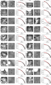 |
Fig. A.1. Twenty galaxies labelled as nucleated in this work (see Sect. 2.3). Column 1 (4) shows the galaxy images with widths of 5Re, with the galaxy stellar masses annotated. Column 2 (5) shows the residual images (widths of 10 arcsec) based on the multi-component models without a nucleus component. Column 3 (6) shows the galaxy surface brightness from individual pixels (grey) and the azimuthally averaged surface brightness profiles from multi-component models with (red) and without (black) a nucleus component. |
Appendix B: Completeness
Broadly speaking, the limit in detecting nuclei boils down to the surface brightness contrast of the nucleus to its host galaxy: the higher the nucleus contrast, the easier it is to detect. It is worth noting that the nucleus contrast is dependent on the seeing of the data: as the nuclei are unresolved in the FDS, the true nucleus contrast will be much higher than what we obtain in this work. In data with better seeing, the light of the nuclei will be spread over fewer pixels, whilst the underlying galaxy light will not differ drastically, leading to higher nucleus contrasts. As we discuss in Appendix B.1, the dependence of nucleus contrast on the spatial resolution impacts the lowest nucleus mass that can be detected.
Another point to consider is that the nucleus contrast is affected by certain factors that dominate at different masses. In massive galaxies, the nucleus tends to reside alongside bright stellar structures (e.g. bulges, bars). As a result, the surface brightness profiles typically rise sharply in the inner regions of the galaxies. The brighter the structures, the lower the nucleus contrasts, making them more difficult to detect. Of the 20 galaxies we identify as nucleated in this work, the 13 more massive galaxies (M* > 109 M⊙) exhibit bright, complex structures14. On the low-mass end of the spectrum, dwarfs are generally not as centrally concentrated (Sérsic n ≲ 1) and do not exhibit as many stellar structures as massive galaxies. However, both the dwarfs and their nuclei tend to be very faint, so the signal-to-noise ratio (S/N) becomes the limiting factor in detecting nuclei. Given the importance of the contrast in detecting nuclei, here we explore the contrast of our sample of nuclei.
To estimate the apparent nucleus contrast, we define it as the flux ratio of the nucleus to the underlying central galaxy flux within a circular aperture with an FWHM radius:
where fnuc is the nucleus total flux, and fgalaxy, aper is the galaxy flux within the FWHM aperture (excluding the nucleus component). In order to compare the apparent nucleus contrast between the nucleated and non-nucleated galaxies in our sample, we used their multi-component models (which include the added nucleus component for the non-nucleated galaxies) to calculate the apparent nucleus contrasts.
In Fig. B.1, we find that, as expected, the galaxies we labelled as nucleated have higher nucleus contrast than the non-nucleated galaxies. Moreover, we find that the average nucleus contrast is higher for low-mass nucleated galaxies than their higher mass counterparts, although the spread is larger at lower masses and the sample size is more modest at higher masses. Furthermore, of the non-nucleated galaxies, those with ΔBIC > 0 generally have higher nucleus contrast than those with ΔBIC < 0. The higher average values for ΔBIC > 0 compared to ΔBIC < 0 implies that the BIC most likely (indirectly) take the nucleus contrast into account. For a galaxy with a very low apparent nucleus contrast, the additional nucleus component would not affect the residual (and hence χ2) as much as the penalisation for including the additional component. For ΔBIC < 0, the rapid decrease in the moving average is due to a lack of a significant nucleus component in the majority of their multi-comp models. Despite the differences in the moving averages, there is a clear overlap between the sub-samples at low galaxy stellar masses (< 107 M⊙). There is not a clear constant limit that can delineate the nucleated from the non-nucleated sub-samples. Instead, the apparent limit appears to increase with decreasing galaxy stellar mass, which is likely a result of the S/N on the apparent nucleus contrast, before increasing at the highest mass end. In Fig. B.2, we show the nucleus flux fraction as a function of galaxy stellar mass and overlay the detection limits due to the S/N (see Sect. B.1).
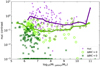 |
Fig. B.1. Nucleus contrast as a function of galaxy stellar mass. The violet dots show the nucleated galaxies, whereas the green circles and crosses denote the non-nucleated galaxies with ΔBIC > 0 and ΔBIC < 0, respectively. The newly identified nucleated galaxies possess both the ΔBIC > 0 and nucleated symbols. For comparison, the solid lines show the moving averages for the nucleated and ΔBIC > 0 sub-samples. Those with nucleus contrast below 10−3 are shown as triangles along the x-axis. |
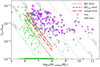 |
Fig. B.2. Similar to Fig. 15, but based on multi-component models. The marker size denotes the nucleus contrast (i.e. larger markers denote higher contrasts). |
B.1. Detection limit
To quantify the effects of low S/N in detecting nuclei, we first explored the BIC and BICres by testing their effectiveness in detecting nucleus components in a controlled manner. To do so, we first created synthetic galaxy images with a range of galaxy stellar masses (106 M⊙ < M∗,galaxy < 108 M⊙) and nucleus stellar masses (104 M⊙ < M∗,nuc < 105 M⊙). We modelled each synthetic galaxy with a single Sérsic for the disc component and a PSF for the nucleus component. To ensure the synthetic galaxies appear realistic for a given galaxy stellar mass, we calculated and use the scaling relations of Sérsic parameters based on the Sérsic+PSF decomposition models (i.e. the moving averages in Fig. E.1). The galaxy stellar mass was converted to total r′ band magnitude via moving averages, whereas the nucleus total magnitude was calculated using the following approximation:
where M*, nuc/M*, galaxy denotes the nucleus stellar mass fraction and fnuc/fgalaxy is the ratio of nucleus to galaxy total fluxes. Each nucleus component was placed at the centre of the galaxy, creating synthetic images of nucleated galaxies. All the synthetic galaxies have a face-on orientation and include realistic FDS noise based on their sigma images (constructed from the expected instrumental and photon noises).
For each galaxy, we conducted single Sérsic and Sérsic+PSF decompositions to calculate their ΔBIC values for BIC and BICres. The point at which ΔBIC< 0 implies that the method does not find significant improvement in fitting the Sérsic+PSF model over the single Sérsic model at the given nucleus stellar mass. In other words, the method does not find a nucleus, and a nucleus of this stellar mass would not be detected in our sample. In Fig. B.3, we show the ΔBIC values for a grid of galaxy and nucleus stellar masses. We find a weak trend in the nucleus and galaxy stellar mass: ΔBIC = 0 for BIC and BICres, such that the detection limit can be approximated as M*, nuc ≈ 104.2 M⊙ for the BIC, and M*, nuc ≈ 104.8 M⊙ for BICres for dwarfs. In Fig. B.4, we show the synthetic nucleated galaxies with M*, galaxy = 107 M⊙ and different M*, nuc, including the limiting cases. In principle, the BIC method of nucleus detection alone should be complete down to M*, nuc ≳ 104.2 M⊙. However, this should be considered as a lower limit due to the simplicity of the synthetic galaxies and the closeness of the galaxy structures to the functions used in the decompositions. In practice, the detection limit is likely closer to the limit from visual inspections. From visual inspection of the images and residuals of the synthetic galaxies, we estimate the limit to be M*, nuc ≈ 104.5 M⊙. It is worth noting that we do not account for other factors such as extinction due to dust, which can increase the nucleus detection limit. Moreover, our estimated detection limits are likely constrained by the seeing of our data. For high-resolution data, such as from the HST, it is likely that the higher nucleus contrast would be able to push the nucleus detection limit to lower masses than in this work. In the context of the GC in-spiral formation channel, the lowest mass nuclei in our sample are already comparable to low-mass GCs. However, it is uncertain if lower mass GCs can survive the process of dynamical friction towards the galaxy centre before they evaporate (due to tidal stripping of stars; see e.g. Fujii et al. 2006). The question of whether lower mass nuclei can exist in low-mass dwarfs requires further investigation with high-resolution data.
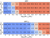 |
Fig. B.3. ΔBIC values for BIC (upper) and BICres (lower) of synthetic nucleated galaxies with varying nucleus and galaxy stellar masses. The ΔBIC values are annotated in each square. ΔBIC> 0 (red) implies that a nucleus of the given stellar mass would be detected, whereas ΔBIC< 0 (blue) would not be detected. The dashed vertical lines denote the jump between nucleated and non-nucleated synthetic galaxies. |
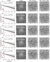 |
Fig. B.4. Examples of synthetic nucleated galaxies with M*, galaxy = 107 M⊙ and various M*, nuc (see the middle rows of Fig. B.3). The first column shows the surface brightness profiles, where the grey points denote the surface brightness from individual pixels of the images. The galaxy (black), nucleus (red), and combined (white) profiles come from the Sérsic+PSF models. The second column shows the inner Re of the galaxy with 27 > μ > 22 mag arcsec−2, with the nucleus contrast (Eq. B.1) annotated. The third and fourth columns show the residual images from subtracting the single Sérsic and Sérsic+PSF models, respectively. The BIC values for each model are annotated in the images. The detection limits for the BIC, visual inspection, and BICres are estimated as 104.2 M⊙, 104.5 M⊙, and 104.8 M⊙, respectively. |
Appendix C: Comparison of nucleation with ACSFCS
Here, we compare our nucleation label with that of the ACSFCS, specifically the work of Turner et al. (2012), which focused on the nucleation of 43 early-type galaxies with BT ≤ 15.5 from the FCC. We first cross-matched the galaxies with our sample and find that nine of the ACSFCS galaxies are not in our catalogue (FCC026, FCC043, FCC063, FCC095, FCC152, FCC204, FCC324, IC2006, NGC1340), either because they are not within the FDS coverage or they were not deemed cluster members in the selection cuts of Venhola et al. (2018). Of the remaining 34 matched galaxies, we find that they are massive (108.7 M⊙ < M* < 1011.4 M⊙), and the majority (26) exhibit stellar structures, such as bulges and bars, based on our multi-component models. In total, we find that the nucleation labels agree for 29 out of 34 galaxies, and of those that are nucleated, their nuclei are relatively massive (< M*, nuc > = 107.1 ± 0.6 M⊙). In Table C.1, we list the five galaxies with differing nucleation labels, and our remarks for each case. Additionally, we show their galaxy images as well as the residuals from the multi-component models with and without a nucleus component in Fig. C.1. Overall, the agreement between our nucleation label and those of Turner et al. (2012) suggests that our nucleation detection is robust.
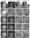 |
Fig. C.1. Five galaxies with opposing nucleation labels between Turner et al. (2012) and this work. We show our galaxy images from the FDS (column 1) and the ACSFCS (column 2), as well as the residuals based on the multi-component models with (column 3) and without (column 4) a nucleus component. The nucleation labels from Turner et al. (2012) and this work are annotated in column 2 and column 3, respectively (Y=nucleated, N=non-nucleated). The white regions denote masked regions. All the images have widths of 20 arcsec. |
Comparison of nucleation with Turner et al. (2012).
Appendix D: Uncertainty of nucleus colours
To estimate the uncertainty in the nucleus magnitudes, we considered two sources: the S/N and the PSF model. The first source is most prominent for faint nuclei, where the low S/N can affect the best-fit nucleus magnitude. We estimated this uncertainty by taking the formal GALFIT uncertainties. The second source of uncertainty comes from the PSF model used to fit the nuclei. To estimate this uncertainty, we created a new set of PSFs in the g′, r′, and i′ bands for each nucleated galaxy to use in decompositions. The new PSFs were created by first producing a catalogue of sources using Source Extractor on (Bertin & Arnouts 1996) the galaxy postage stamp images. The catalogue was then used as an input for PSF Extractor (PSFEx, Bertin 2011), which selects suitable sources to model the PSF from. We configured PSFEx to select sources with 3 pix < SAMPLE_FWHMRANGE < 12 pix, SAMPLE_VARIABILITY = 0.2, SAMPLE_MINSN = 10, and SAMPLE_MAXELLIP = 0.2, and the resulting PSF is over-sampled by a factor of 2 (i.e. PSF_SAMPLING = 0.5). In principle, the resultant PSFs from PSFEx can be used for decompositions, but the limited number of selected sources from some postage stamp images led to clear non-axisymmetric variations. To proceed, we fitted 2D Gaussians to the resultant PSFs from PSFEx to create smooth, axisymmetric PSFs, with which were re-ran the multi-component decompositions.
In Fig. D.1, we compare the PSFs created in Su et al. (2021) and the Gaussian fits. Both PSFs are axisymmetric and appear to be very similar within the HWHM, but they differ at larger radii due to the extended tail of the Su et al. (2021) PSF. As a result, the nucleus magnitudes derived from Gaussian PSFs are systematically fainter than the magnitudes from the extended PSFs. However, the systematic offsets cancel out when we calculate the colours (see Fig. D.2), so we estimated the uncertainty in nucleus colours as the difference in colours derived from the decompositions using the two different PSFs.
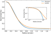 |
Fig. D.1. Comparison of PSF profiles from FDS25 field (orange; from Su et al. 2021) and the Gaussian fits from the postage stamp image of FDS25_0000 (blue) in the r′ band. The small inset plot shows the profiles in logarithmic axes. |
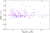 |
Fig. D.2. Nucleus g′−r′ colour derived from Su et al. (2021) PSFs minus the colour derived from the Gaussian PSFs for each nucleated galaxy, as a function of nucleus stellar mass (same as in Fig. 19) for all nucleated galaxies in our sample. Nuclei with values beyond the axis limits are denoted as triangles along the x-axes. |
Appendix E: Early-type galaxy properties
In Fig. E.1, we show the host galaxy quantities of early-type nucleated and non-nucleated galaxies for which the p values are > α, which implies that the null hypothesis (that the two sub-samples are drawn from the same distribution) cannot be rejected with confidence for these quantities. We also include the concentration index C, which did have p values < α, but this is most likely due to the fact that the nuclei were included in the calculations of C.
All Tables
All Figures
|
Fig. 1. Overview of Fornax galaxies, split between Fornax main cluster (blue) and Fornax A group (orange). The dashed circles denote the virial radius for the Fornax main cluster (∼2 deg = 0.7 Mpc) and the Fornax A group (∼1 deg = 0.35 Mpc) (Drinkwater et al. 2001). The black dots denote galaxies with a nucleus. |
| In the text | |
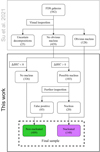 |
Fig. 2. Flow chart of our final galaxy sample. See Sect. 2.3 for details. |
| In the text | |
|
Fig. 3. Histograms of host galaxy stellar masses for nucleated (violet) and non-nucleated (green) galaxies in the Fornax main cluster and Fornax A group. The dashed histogram denotes the distribution of newly identified nucleated galaxies (see Sect. 2.3). Bins with widths of 0.5 dex were used. |
| In the text | |
|
Fig. 4. Examples of BIC false positives (i.e. ΔBIC > 0 but no nucleus). We show the images (left) and residuals based on the multi-component model without (centre) and with (right) a nucleus component. The white regions denote masked regions. The images in the first column have widths of 4Re and surface brightness limits from 18–27 mag arcsec2, whereas the residual images have widths of 20 arcsec and are limited from –1 to 1 mag arcsec2 in surface brightness. The red circles have a radius of the average PSF FWHM × 2. The galaxy stellar masses are annotated in the first column. |
| In the text | |
|
Fig. 5. Nucleation fraction as a function of host galaxy stellar mass for the Fornax main cluster (blue) and the Fornax A group (orange). The shaded regions denote the 68% binomial confidence interval based on the Wilson score interval (Wilson 1927). For both sub-samples, a bin width of 1 dex was used and the number of galaxies per bin is labelled in the plot. Due to the low number of galaxies, we omit bins with M* > 1010 M⊙ from the Fornax A group and M* > 1011 M⊙ from the Fornax main cluster. |
| In the text | |
|
Fig. 6. Nucleation fraction between the Fornax main cluster (blue) and the Fornax A group (orange) as a function of projected distance (using NGC1399 and NGC1316 as the centre for the Fornax main cluster and Fornax A group, respectively). The shaded regions denote the 68% binomial confidence interval. The number of galaxies in each bin are annotated in the plot. The dashed vertical lines denote the same limits as in Fig. 1. |
| In the text | |
|
Fig. 7. g′−r′ (upper) and g′−i′ (lower) as a function of host galaxy stellar mass. Filled circles are galaxies with nucleus contrast > 1, whereas open circles denote those with nucleus contrast < 1. The marker size denotes the nucleus contrast (see Eq. (B.1)), with bigger points denoting higher nucleus contrast. The solid lines denote the moving (median) averages of the solid points, which were calculated using a bin width of 2 dex, and moved in steps of 0.2 dex. The shaded regions denote the corresponding standard error of the mean (SEM) in the moving averages. Nuclei with values beyond the axis limits are denoted as triangles along the x-axes. The individual error bars were estimated in Appendix D. |
| In the text | |
|
Fig. 8. Nucleus g′−r′ colour as a function of nucleus contrast (see Eq. (B.1)) for nuclei of early-type galaxies. The marker size denotes the nucleus contrast. The dotted vertical line denotes the limit of nucleus contrast = 1, which loosely separates nuclei with high and low scatter in colour. |
| In the text | |
|
Fig. 9. Difference in colour between nucleus and its host galaxy as a function of the host galaxy stellar mass. We show both g′−r′ (pink) and g′−i′ (gold) colours based on the multi-component decomposition models. The moving averages were calculated using a bin width of 2 dex and moved in steps of 0.2 dex. The shaded regions denote the SEM. The marker size denotes the nucleus contrast. The uncertainties were estimated by propagating the nuclei colour uncertainties (see Appendix D) and the galaxy colour uncertainties calculated in Su et al. (2021; see their Table 1). |
| In the text | |
|
Fig. 10. Similar to Fig. 7, but showing the difference in colour between the nucleus and its host galaxy as a function of the projected distance. The marker size denotes the nucleus contrast. Unlike Fig. 7, here we only show galaxies in the Fornax main cluster. |
| In the text | |
|
Fig. 11. Nucleus stellar mass as a function of the host galaxy stellar mass. We applied two estimates for the nucleus stellar mass: from r′ band nucleus flux fractions (violet) and Eq. (1) (light brown). The linear fits for both estimates are shown as solid lines. For comparison, we also include the relations from Neumayer et al. (2020; their Eq. (1)) and Georgiev et al. (2016; their early-type sample) as dashed and dash-dotted black lines. The nucleus stellar mass based on Eq. (1) for FDS12_0367 and FDS15_0232 have been omitted due to too faint g′ and i′ band nucleus magnitudes. |
| In the text | |
|
Fig. 12. Nucleus flux fraction as a function of host galaxy stellar mass for all nucleated early-type galaxies. The moving average (violet) was calculated using a bin width of 2 dex, and moved in steps of 0.2 dex (based on log10(fnuc/ftotal) instead). The shaded region denotes the 1σ uncertainty within the moving average bins. The dashed and dot-dashed black lines denote the relation from Neumayer et al. (2020; their Eq. (1)) and Georgiev et al. (2016; their early-type sample), respectively. The dotted and dot-dashed red lines denote the estimated detection limits based on BIC and visual inspection, respectively. The dotted grey lines denote constant nucleus stellar masses. |
| In the text | |
|
Fig. 13. Structural quantities of the nucleated (violet) and non-nucleated (green) early-type galaxies in the Fornax main cluster and Fornax A group. Column (1): structural quantities as functions of the galaxy stellar mass. The black lines denote the moving averages (median). Column (2): residual quantities, calculated as the measured quantities minus moving average from Col. (1). The solid lines denote the moving averages of the residual quantities. The dashed grey vertical lines denote the range where both samples overlap in stellar mass. Column (3): histograms of the residual quantities between nucleated and non-nucleated galaxies within the overlapping stellar mass range. The coloured dotted lines denote the median value of each sub-sample. For brevity, here we show quantities of interest. The full plot with all considered quantities can be found in Appendix E. |
| In the text | |
|
Fig. 14. Residual |
| In the text | |
|
Fig. 15. Nucleus flux fraction as a function of host stellar mass, based on Sérsic+PSF models. Nucleated galaxies are shown in violet and non-nucleated galaxies are shown in green. Those with a fitted nucleus total magnitude of 35 mag are shown as triangles along the x-axis. The dotted, dot-dashed, and dashed red lines are the estimated BIC, visual, and BICres detection limits, respectively, based on our synthetic nucleation tests (see Sect. B.1). |
| In the text | |
|
Fig. 16. Accuracy of BIC (upper) and BICres (lower) in classifying nucleated and non-nucleated early-type galaxies. True (i.e. correct) and false (i.e. incorrect) classifications are denoted by circles and crosses, respectively. Galaxies where GALFIT fails to find a nucleus (i.e. the triangles from Fig. 15) have been omitted. The BIC classification accuracies are shown in Table 4. |
| In the text | |
|
Fig. 17. Comparison of different NSC formation mechanisms with our nucleated early-type galaxies. The violet points, solid line, and shaded region denote our nucleated galaxies (same as in Fig. 12). We consider the maximum NSC mass via tidal compression of gas (i.e. an upper limit; red; Emsellem & van de Ven 2008), GC in-spiral (orange and cyan; Gnedin et al. 2014 and Antonini et al. 2015, respectively), and a combination of GC in-spiral and galaxy evolution models (blue; Antonini et al. 2015). The black hole scaling relation (green; Greene et al. 2020) is included to illustrate the evolution of black holes. The dotted portion of the coloured lines denote an extrapolation of the original relation. The dotted grey lines denote constant nucleus stellar masses. |
| In the text | |
|
Fig. 18. Structural quantities of nucleated (violet) and non-nucleated (green) early-type galaxies in the Fornax main cluster only, as a function of the projected distance. Only galaxies with overlapping stellar mass are shown (i.e. Col. (4) from Fig. 13). The measured (left) and residual (i.e. mass-trend corrected; right) quantities are shown. The solid lines are based on linear fits to the data and are only meant as visual guides to the Spearman’s rank correlation coefficient, rs. For each quantity, the rs and associated p values are annotated in the corresponding sub-plots. |
| In the text | |
|
Fig. 19. g′−r′ colour as a function of stellar mass for GCs (grey), UCDs (crimson), and nuclei (violet). As in Fig. 7, the nuclei with nucleus contrast > 1 are shown as filled circles, whereas nuclei with nucleus contrast < 1 are shown as open circles. The upper and right panels show the stellar mass and g′−r′ distributions, respectively. The nuclei uncertainties are the same as in Fig. 7. The UCD uncertainties are generally within the size of the points, and hence they are omitted. |
| In the text | |
|
Fig. 20. Distribution of projected cluster-centric distance for GCs (grey), UCDs (crimson), and nuclei (violet). Here, only nuclei from early-type galaxies in the Fornax main cluster are shown. The upper panel shows the cumulative distribution of all the compact objects, respectively. The lower panel shows the cumulative distributions of the low- (dotted) and high- (dashed) mass sub-samples of UCDs split at M* = 106.6 M⊙ and the nuclei within the accompanying UCD stellar mass ranges. The dotted blue line denotes the virial radius of the Fornax main cluster. |
| In the text | |
|
Fig. 21. UCD fraction (fUCD = NUCD/(NUCD + Nnuc)) as a function of projected cluster-centric distance for the Fornax (blue) and Virgo (black) clusters. We used a virial radius of 1.55 Mpc for the Virgo cluster (Ferrarese et al. 2012). The shaded regions show the 1σ binomial uncertainty. The dotted and dash-dotted green lines show the predicted UCD fractions depending on whether the UCD progenitor galaxies contain gas or not, respectively. |
| In the text | |
|
Fig. A.1. Twenty galaxies labelled as nucleated in this work (see Sect. 2.3). Column 1 (4) shows the galaxy images with widths of 5Re, with the galaxy stellar masses annotated. Column 2 (5) shows the residual images (widths of 10 arcsec) based on the multi-component models without a nucleus component. Column 3 (6) shows the galaxy surface brightness from individual pixels (grey) and the azimuthally averaged surface brightness profiles from multi-component models with (red) and without (black) a nucleus component. |
| In the text | |
|
Fig. B.1. Nucleus contrast as a function of galaxy stellar mass. The violet dots show the nucleated galaxies, whereas the green circles and crosses denote the non-nucleated galaxies with ΔBIC > 0 and ΔBIC < 0, respectively. The newly identified nucleated galaxies possess both the ΔBIC > 0 and nucleated symbols. For comparison, the solid lines show the moving averages for the nucleated and ΔBIC > 0 sub-samples. Those with nucleus contrast below 10−3 are shown as triangles along the x-axis. |
| In the text | |
|
Fig. B.2. Similar to Fig. 15, but based on multi-component models. The marker size denotes the nucleus contrast (i.e. larger markers denote higher contrasts). |
| In the text | |
|
Fig. B.3. ΔBIC values for BIC (upper) and BICres (lower) of synthetic nucleated galaxies with varying nucleus and galaxy stellar masses. The ΔBIC values are annotated in each square. ΔBIC> 0 (red) implies that a nucleus of the given stellar mass would be detected, whereas ΔBIC< 0 (blue) would not be detected. The dashed vertical lines denote the jump between nucleated and non-nucleated synthetic galaxies. |
| In the text | |
|
Fig. B.4. Examples of synthetic nucleated galaxies with M*, galaxy = 107 M⊙ and various M*, nuc (see the middle rows of Fig. B.3). The first column shows the surface brightness profiles, where the grey points denote the surface brightness from individual pixels of the images. The galaxy (black), nucleus (red), and combined (white) profiles come from the Sérsic+PSF models. The second column shows the inner Re of the galaxy with 27 > μ > 22 mag arcsec−2, with the nucleus contrast (Eq. B.1) annotated. The third and fourth columns show the residual images from subtracting the single Sérsic and Sérsic+PSF models, respectively. The BIC values for each model are annotated in the images. The detection limits for the BIC, visual inspection, and BICres are estimated as 104.2 M⊙, 104.5 M⊙, and 104.8 M⊙, respectively. |
| In the text | |
|
Fig. C.1. Five galaxies with opposing nucleation labels between Turner et al. (2012) and this work. We show our galaxy images from the FDS (column 1) and the ACSFCS (column 2), as well as the residuals based on the multi-component models with (column 3) and without (column 4) a nucleus component. The nucleation labels from Turner et al. (2012) and this work are annotated in column 2 and column 3, respectively (Y=nucleated, N=non-nucleated). The white regions denote masked regions. All the images have widths of 20 arcsec. |
| In the text | |
|
Fig. D.1. Comparison of PSF profiles from FDS25 field (orange; from Su et al. 2021) and the Gaussian fits from the postage stamp image of FDS25_0000 (blue) in the r′ band. The small inset plot shows the profiles in logarithmic axes. |
| In the text | |
|
Fig. D.2. Nucleus g′−r′ colour derived from Su et al. (2021) PSFs minus the colour derived from the Gaussian PSFs for each nucleated galaxy, as a function of nucleus stellar mass (same as in Fig. 19) for all nucleated galaxies in our sample. Nuclei with values beyond the axis limits are denoted as triangles along the x-axes. |
| In the text | |
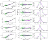 |
Fig. E.1. Same as Fig. 13, but for the host properties for which the p values are > α. |
| In the text | |
Current usage metrics show cumulative count of Article Views (full-text article views including HTML views, PDF and ePub downloads, according to the available data) and Abstracts Views on Vision4Press platform.
Data correspond to usage on the plateform after 2015. The current usage metrics is available 48-96 hours after online publication and is updated daily on week days.
Initial download of the metrics may take a while.