| Issue |
A&A
Volume 664, August 2022
|
|
|---|---|---|
| Article Number | A110 | |
| Number of page(s) | 17 | |
| Section | Extragalactic astronomy | |
| DOI | https://doi.org/10.1051/0004-6361/202142228 | |
| Published online | 12 August 2022 | |
Properties of IR-selected active galactic nuclei
1
Instituto de Astronomía Teórica y Experimental, (IATE, CONICET-UNC), Córdoba, Argentina
e-mail: This email address is being protected from spambots. You need JavaScript enabled to view it.
2
Observatorio Astronómico de Córdoba, Universidad Nacional de Córdoba, Laprida 854, X5000BGR Córdoba, Argentina
Received:
15
September
2021
Accepted:
29
March
2022
Abstract
Context. Active galactic nuclei (AGNs) of galaxies play an important role in the life and evolution of galaxies through the impact they exert on certain properties and on the evolutionary path of galaxies. It is well known that infrared (IR) emission is useful for selecting galaxies with AGNs, although it has been observed that there is contamination by star-forming galaxies.
Aims. We investigate the properties of galaxies that host AGNs that are identified at mid- (MIR) and near-IR wavelengths. The sample of AGNs selected at IR wavelengths was confirmed using optical spectroscopy and X-ray photometry. We study the near-UV, optical, near-IR and MIR properties, as well as the [O III] λ5007 luminosity, black hole mass, and morphology properties of optical and IR colour-selected AGNs.
Methods. We selected AGN candidates using two MIR colour selection techniques: a power-law emission method, and a combination of MIR and near-IR selection techniques. We confirmed the AGN selection with two line diagnostic diagrams that use the ratio [O III]/Hβ and the emission line width σ[O III] (kinematics–excitation diagram, KEx) and the host galaxy stellar mass (mass–excitation diagram, MEx), as well as X-ray photometry.
Results. According to the diagnostic diagrams, the methods with the greatest success in selecting AGNs are those that use a combination of a mid- and near-IR selection technique and a power-law emission. The method that uses a combination of MIR and near-IR observations selects a large number of AGNs and is reasonably efficient in the success rate (61%) and total number of AGNs recovered. We also find that the KEx method presents contamination of star-forming galaxies within the AGN selection box. According to morphological studies based on the Sérsic index, AGN samples have higher percentages of galaxy morphologies with bulge+disk components than galaxies without AGNs.
Key words: galaxies: active / infrared: galaxies / quasars: emission lines
© ESO 2022
1. Introduction
Active galactic nuclei (AGN) are compact regions at the centre of massive galaxies, perhaps in all of them, that emit large amounts of radiation of non-thermal origin. The origin of this large energy emission has been connected with the presence of a massive black hole at the centre of the galaxies (Zel’dovich & Novikov 1964; Rees 1984). Since their discovery (Schmidt 1963), AGNs have become a fundamental part of understanding the origin and evolution of galaxies. The identification is fundamental for the study of host galaxy properties and to study the evolutionary processes that galaxies undergo throughout their lives. The connection between various parameters related to the black hole and its host galaxy is well known, although their physical sizes differ by several orders of magnitude. This includes the relation between the black hole mass and the bulge mass (Magorrian et al. 1998; Wandel 1999; McLure & Dunlop 2000; Häring & Rix 2004; Graham & Scott 2015; Ding et al. 2020), between black hole mass and the velocity dispersion (Ferrarese & Merritt 2000; Gebhardt et al. 2000; Merritt & Ferrarese 2001; Beifiori et al. 2012), and even also with the host galaxy mass (Bandara et al. 2009).
Some studies showed that the selection of AGNs in the UV, optical, and even in X-ray surveys missed several relatively dust-obscured AGNs and almost the entire heavily obscured Compton-thick AGN population (Gilli et al. 2007; Daddi et al. 2007; Treister et al. 2009). It is well known that the selection in the infrared (IR) is a potentially powerful way to identify a variety of AGNs, including obscured AGNs (Hickox & Alexander 2018, and references therein). Moreover, the spectral energy distribution (SED) of AGNs in the mid-IR (MIR) is very different from that of normal galaxies and stars (Assef et al. 2018). According to the observed redshift range, the emission in the IR can come from structures close to the black hole, such as the torus (observed at low redshifts, i.e. z ≤ 1.5) as well as from the accretion disk (at z ≥ 1.5, Chung et al. 2014; Assef et al. 2018). After the advent of the Spitzer Space Telescope, large samples of AGNs could be obtained with the IRAC camera, which operated with filters centred at [3.6], [4.5], [5.8], and [8.0] μm (Lacy et al. 2004; Stern et al. 2005; Hickox et al. 2007; Donley et al. 2007, 2008, 2012; Park et al. 2010; Assef et al. 2011; Mendez et al. 2013; Bornancini et al. 2017; Chang et al. 2017; Bornancini & García Lambas 2018, 2020). The first investigations include Eisenhardt et al. (2004), who discovered a sequence of objects in the [3.6]−[4.5] vs. [5.8]−[8.0] colour–colour diagram formed by compact objects identified in the [3.6] μm filter. Preliminary spectroscopy of these unresolved sources suggested that they are a mixture of broad-lined quasars (QSOs) and starburst galaxies (Eisenhardt et al. 2004). Following this idea, Lacy et al. (2004) identified the position of QSOs detected in the Sloan Digital Sky Survey (SDSS) in a log(S8.0/S4.5) vs. log(S5.8/S3.6) (where Sν is the flux density at the frequency ν) diagram and presented a colour-cut criterion in order to select them. Another well-known MIR-based method of AGN selection was that presented by Stern et al. (2005). These authors used a similar approach to establish an empirical criterion to separate active galaxies from other sources based on the distribution of nearly 10 000 spectroscopically identified sources from the AGN and Galaxy Evolution Survey (Kochanek et al. 2012). It is well known that in MIR spectra, AGNs are often characterised by a power law (Sν ∝ να, where α is the spectral index) in their SEDs at rest-frame optical, near-IR, and MIR wavelengths (Neugebauer et al. 1979; Elvis et al. 1994; Alonso-Herrero et al. 2006; Donley et al. 2007; Chang et al. 2017). This emission may be caused by non-thermal processes in the nuclear region and by thermal emission due to various nuclear dust components (Rieke & Lebofsky 1981).
The optical and UV light emitted by the accretion disk located near the black hole is absorbed by a dust structure around them, which reprocesses it and re-emits the radiation at IR wavelengths. According to the unified model (Antonucci 1993; Urry & Padovani 1995), this structure formed by dust would have the appearance of a torus, although several studies suggested that the shape is not so regular (Alonso-Herrero et al. 2011; Audibert et al. 2017), and it could even have considerable sizes (Goulding et al. 2012; Donley et al. 2018). The re-emission of the radiation produced can be described with a power law from 1 to 10 μm (which is the coverage sampled by the four IRAC filters), showing a thermal bump that peaks around 10 μm. Some authors stated that AGNs have a variety of slopes ranging from α = −1 for selected QSOs in the optical (Elvis et al. 1994), while others suggested that QSOs have indices ranging from −0.5 to −2 (Ivezić et al. 2002; Barmby et al. 2006). In star-forming (SF) galaxies, they were expected to have α ≃ +2 (Barmby et al. 2006). This method was used by several authors to select samples of AGNs (Lacy et al. 2004, 2007; Alonso-Herrero et al. 2006; Polletta et al. 2006; Donley et al. 2007, 2008, 2012; Park et al. 2010; Chang et al. 2017; Bornancini & García Lambas 2020).
It is well known that some IR-selection methods for AGNs also select other galaxy types as contaminants and also fail to detect some AGN types. Mendez et al. (2013) studied the Spitzer/IRAC and X-ray selection methods for AGNs identified in four large fields, the Cosmological Evolution Survey (COSMOS, Scoville et al. 2007), the XMM Large Scale Structure survey (XMM-LSS, Pierre et al. 2004), the European Large Area Infrared Space Observatory (ES1-S1, Oliver et al. 2000), and the Chandra Deep Field South (CDFS, Giacconi et al. 2001) surveys. They found that the selected sample of galaxies according the Stern et al. (2005) method is contaminated by SF galaxies at z ∼ 0.3 and by quiescent galaxies at z ∼ 1.1. As noted by Donley et al. (2012), the two selection methods proposed by Lacy et al. (2007) and Stern et al. (2005) are contaminated by galaxies that are classified as pure starburst galaxies as determined by Spitzer InfraRed Spectrograph observations. Although the effect is greater at high redshifts, it is also observed for galaxies in the redshift range of 0.5 < z < 1. Based on simulations, Sajina et al. (2005) found higher contamination from intermediate-redshift sources dominated by polycyclic aromatic hydrocarbon near the limits of the Lacy et al. (2004) AGN selection region. They are commonly identified with a wide variety of objects, including dusty starbursts and quiescent and low-metallicity galaxies. Georgantopoulos et al. (2008) found that AGN selection methods based on either colours or power-law spectra would fail to detect a large fraction of Compton-thick AGN candidates. In a similar way, Park et al. (2010) analysed the properties of power-law and X-ray emission from AGNs and found that only 22% of the X-ray AGNs are detected by the power-law AGN selection method.
In this paper we analyse the properties of galaxies hosting AGNs that are identified at IR wavelengths and were confirmed by means of optical spectroscopy and X-ray photometry. We use four MIR and near-IR methods according to the criteria of Lacy et al. (2004), Stern et al. (2005), Chang et al. (2017), and Messias et al. (2012) and two line diagnostic diagrams that use the quotient [O III]/Hβ and the emission line width σ[O III] (Zhang & Hao 2018) and the host galaxy stellar mass (Juneau et al. 2014).
This paper is organised as follows: In Sect. 2 we present all datasets we used, and in Sect. 3 we detail the different MIR and near-IR (Ks) AGN selection methods. In Sect. 4 we analyse the KEx and MEx line diagnostic diagrams for AGNs. In Sect. 5 we explore the X-ray emission and the different MIR and near-IR methods and line diagnostic diagram properties for AGNs. We study the properties of AGNs selected by KEx and MEx diagnostic diagrams in Sect. 6. In Sect. 7 we study the X-ray properties, black hole mass, accreting properties, and the morphology of AGNs selected through the MEx diagram. Finally, the summary and discussion of our study are presented in Sect. 8.
We use the AB magnitude system throughout (Oke & Gunn 1983) and assume a ΛCDM cosmology with H0 = 70 km s−1 Mpc−1, ΩM = 0.3, and ΩΛ = 0.7.
2. Datasets
Our main goal is to study the galaxy properties of four different MIR and near-IR selection methods and two line diagnostic diagrams that use the emission line quotient [O III]/Hβ and the emission line width σ[O III] (KEx diagram; Zhang & Hao 2018) and [O III]/Hβ vs. stellar mass (MEx diagram; Juneau et al. 2011, 2014). For this study, it is necessary to consider catalogues with spectral data in order to measure line widths and emission line quotients. We selected our AGN sample in the COSMOS field (Scoville et al. 2007) from the COSMOS20151 catalogue (Laigle et al. 2016) and from the zCOSMOS redshift survey (Lilly et al. 2007, 2009). The COSMOS is a deep, wide area, multi-wavelength survey that contains observational information of more than one million galaxies over a 2 square degree region centred at (RA,Dec) = (10h00m28.6s, 2°12′21″). The COSMOS2015 (Laigle et al. 2016) catalogue provides photometric data from 0.24 μm to 500 μm, which includes GALEX FUV and in the near-UV (NUV) observations (Zamojski et al. 2007; Capak et al. 2007); u* observations using the Canada-France-Hawaii telescope (CFHT) and the MegaCam instrument (Sanders et al. 2007); B, V, g, r′, i+, z++ broad bands; IA427, IA464, IA484, IA505, IA527, IA574, IA624, IA679, IA709, IA738, IA767, and IA827, intermediate bands, and NB711, NB816 narrow bands from the COSMOS-20 survey using the Subaru Suprime-Cam (Taniguchi et al. 2007, 2015); near-IR Y, J, H, Ks-band data taken with WIRCam and Ultra-VISTA (McCracken et al. 2010, 2012); six Spitzer IRAC/MIPS bands, 3.6, 4.5, 5.8, 8.0, 24, and 70 μm (Sanders et al. 2007; Le Floc’h et al. 2009; Ashby et al. 2013, 2015), and Herschel PACS/SPIRE 100, 160, 250, 350, and 500 μm (Oliver et al. 2012; Lutz et al. 2011).
zCOSMOS (Lilly et al. 2009) is a large spectroscopic survey obtained through more than 600 hours of observations with the Visible Multi Object Spectrograph (VIMOS) mounted on the Very Large Telescope (VLT) at the European Southern Observatory (ESO) in Chile. This redshift survey is divided into two parts: the zCOSMOS-bright and the zCOSMOS-deep. The first was designed to yield a high and fairly uniform sampling rate (about 70%; Knobel et al. 2012), with a high success rate in measuring redshifts approaching 100% at 0.5 < z < 0.8, covering the approximately 1.7 deg2 of the COSMOS field. The second part, zCOSMOS-deep, observed a small number of galaxies selected to mostly lie at higher redshifts, 1.5 < z < 3.0. We used the last spectroscopic release zCOSMOS (DR3), which contains redshift data from 20 689 galaxies at 0.2 < z < 1.2 selected to have IAB < 22.5 mag. This catalogue provides a full set of extracted one-dimensional spectra, plus a catalogue that contains the 1D spectra filenames, the I-band magnitudes used for the selection, and the measured redshifts and the redshift confidence class parameter.
Several spectroscopic redshift catalogues are available such as DEIMOS 10k (Hasinger et al. 2018), MUSE Wide survey (Urrutia et al. 2019), FMOS-COSMOS (Silverman et al. 2015; Kashino et al. 2019), and the MOSFIRE Deep Evolution Field Survey (Kriek et al. 2015) (see Alarcon et al. 2021 for a complete sample list). We only used the zCOSMOS-bright survey because it represents a homogeneous catalogue using the same selection criteria and with very good completeness.
We first selected sources within the spectroscopic redshift range 0.3 ≤ zsp ≤ 0.9 from the zCOSMOS DR3-bright catalogue with good redshift estimates. This catalogue provides a confident class parameter that includes insecure and probable redshift (class 1 and 2, respectively), one broad AGN redshift (class 18), one line redshift (class 9), and secure and very secure redshifts (class 3 and 4, respectively). Each confidence class is also assigned a confidence decimal, which is derived from repeated observations and for the consistency or otherwise with photometric redshifts. The confidence decimal ranges from .1 (spectroscopic and photometric redshifts are not consistent at the level of 0.04(1 + z)), .3 (special case for classes 18 and 9, consistent with photo-z only after the redshift is changed to the alternative redshift), .4 (no photometric redshift available) to .5, (spectroscopic redshift consistent within 0.04(1 + z) of the photometric redshift). We selected all sources with 3.x and 4.x, where x can take the values 1, 3, 4, and 5. The lower limit of the redshift range we used, which is z = 0.3, corresponds to the limit used by the KEx and MEx line diagnostic diagrams proposed by Zhang & Hao (2018) and Juneau et al. (2014), while the upper limit of z = 0.9 was chosen because it is the detection limit of the observed [OIII]λ5007 line in the spectral range 5550–9450 Å of the VIMOS spectrograph. We call this sample of galaxies with good spectroscopic redshift determinations the zCOSMOS-good; it contains 8633 sources. We then correlated these spectroscopic sources with those of the zCOSMOS15 (Laigle et al. 2016) catalogue in order to obtain the stellar mass (estimated using the MASS_BEST parameter) and other photometric data, such as rest-frame absolute magnitudes MNUV, Mr, MJ, MKs, and the four IRAC bands.
3. MIR and near-IR AGN sample selection
In order to study the selection of AGNs at different MIR and near-IR wavelengths, we used four methods from Lacy et al. (2004), Stern et al. (2005), Chang et al. (2017), and Messias et al. (2012). The first three MIR methods use IRAC bands ([3.6], [4.5], [5.8], and [8.0] μm), and we refer to them throughout the paper as L04, S05, and Ch17, while the method of Messias et al. (2012) (M12) uses a combination of the Ks+IRAC colour criterion (KI criterion). L04 studied the colour distribution of objects according to the flux ratios using the four IRAC bands of the Spitzer Space Telescope: the ratio 8.0/4.5 μm vs. the ratio 5.8/3.6 μm. In this diagram, they separated the objects with blue continua from those with red continua. They observed two clear sequences: one sequence formed by objects with blue colours in S5.8/S3.6 and very red colours in S8.0/S4.5. The first sequence was identified with galaxies at low redshifts (z < 0.2) and the second sequence had red colours in both pairs of filters, and its location matched the region occupied by QSOs identified in the SDSS survey.
In Fig. 1 we plot the 2D density maps representing MIR and near-IR colours for galaxies in the zCOSMOS-good sample. In the left panel we plot the [4.5]−[8.0] vs. [3.6]−[5.8] colour–colour diagram. The dotted line box represents the area proposed by Lacy et al. (2004) to select AGN samples according to the following relation:
 (1)
(1)
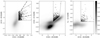 |
Fig. 1. MIR and near-IR colour–colour diagrams and the selection of AGNs for different photometric methods. The left panel shows the criteria of Lacy et al. (2004) (dotted lines) and Chang et al. (2017) (dashed-point lines). The middle panel shows the criterion of Stern et al. (2005), and the right panel shows the criterion of Messias et al. (2012). In each panel we show the 2D density maps that represent galaxies with spectroscopic redshifts with confidence classes 3 and 4 taken from the zCOSMOS DR3 survey. The pre-selected AGNs are represented with black circles. |
where ∧ is the logical AND operator.
In the same panel of the figure, we also plot the Chang et al. (2017) colour–colour cuts of AGNs selected by their MIR power-law emission (dash-dotted line region). They defined power-law sources whose IRAC four-band SEDs are well fit by a line of slope α < −0.5, where Sν ∝ να. These authors defined a selection box that groups the vast majority of AGNs with a power-law emission. We used Fig. 1 of Chang et al. (2017) to obtain limiting lines to define the AGN selection box, which has the following form:
![Mathematical equation: $$ \begin{aligned}&\Bigl ([4.5]{-}[8.0]\Bigr )< 2.22\times \Bigl ([3.6]{-}[5.8]\Bigr )+1.01, \nonumber \\&\Bigl ([4.5]{-}[8.0] < 8.67\times \Bigl ([3.6]{-}[5.8]\Bigr ){-}0.38, \nonumber \\&\Bigl ([4.5]{-}[8.0]>{-}0.27\times \Bigl ([3.6]{-}[5.8]\Bigr )+0.2, \nonumber \\&\Bigl ([4.5]{-}[8.0]\Bigr ) > 0.31\times \Bigl ([3.6]{-}[5.8]\Bigr ){-}0.06. \end{aligned} $$](/articles/aa/full_html/2022/08/aa42228-21/aa42228-21-eq2.gif) (2)
(2)
In the middle panel of Fig. 1, we show the colour–colour [3.6]−[4.5] vs. [5.8]−[8.0] diagram with the selection box represented by dashed lines, showing the selection criterion of Stern et al. (2005). These authors proposed this criterion based on previous results found by Eisenhardt et al. (2004), who noted a vertical spur in the diagram formed mostly by sources that are spatially unresolved in the 3.6 μm images and the location of broad- and narrow-band AGNs selected from the AGEIS survey. These authors proposed the following empirical criteria to separate AGNs from other sources identified in the AEGIS survey2:
![Mathematical equation: $$ \begin{aligned}&\Bigl ([5.8]{-}[8.0] \Bigr )>{-}0.07 \wedge \nonumber \\&\Bigl ([3.6]{-}[4.5]\Bigr )>0.2\times \Bigl ([5.8]{-}[8.0]\Bigr ){-}0.15\wedge \nonumber \\ &\Bigl ([3.6]{-}[4.5]\Bigr )> 2.5\times \Bigl ([5.8]{-}[8.0]\Bigr ){-}2.3. \end{aligned} $$](/articles/aa/full_html/2022/08/aa42228-21/aa42228-21-eq3.gif) (3)
(3)
Finally, the right panel shows the combined near-IR and MIR Ks − [4.5] vs. [4.5]−[8.0] galaxy colours and the selection criteria according to Messias et al. (2012). In the figure, the pre-selected AGNs are represented by black circles. These authors found that this criterion is ideal as AGN/non-AGN diagnostics at z ≲ 1 based on the predictions by the most recent galaxy and AGN templates. The selection criterion is defined by the following simple conditions:
![Mathematical equation: $$ \begin{aligned} \Bigl (K_s-\left[4.5\right]\Bigr )>0 \wedge \Bigl (\left[4.5\right]\!{-}\!\left[8.0\right]\Bigr )>0 \end{aligned} $$](/articles/aa/full_html/2022/08/aa42228-21/aa42228-21-eq4.gif) (4)
(4)
According to these methods, we pre-selected the following number of candidates for AGNs: 490, 78, 362, and 133 sources conforming to the criteria of L04, Ch17, S05, and M12, respectively (see Table 1).
Number of AGN candidates according to the MIR and near-IR methods of L04, Ch17, S05, and M12.
We analyse the completeness of the spectroscopic sample as a function of the IR magnitudes and colours in the appendix.
Donley et al. (2012) presented a different AGN selection criterion according to a power-law emission observed in the IRAC MIR bands. We did not use this method because it only selects a small percentage of AGNs. The area determined by this criterion is smaller and is contained within the selection criteria of Ch17, pre-selecting only 36 AGN candidates.
4. KEx and MEx diagnostic diagrams
Juneau et al. (2011, 2014) and Zhang & Hao (2018) presented the two line diagnostic diagrams to classify and separate AGNs from star-forming and composite galaxies. First, Juneau et al. (2011) introduced the MEx diagnostic diagram to identify AGNs in galaxy samples at intermediate redshift. These authors used a modified version of the Baldwin–Phillips–Terlevich (BPT; Baldwin et al. 1981) diagram, which involves [N II] λ6584/Hα and [O III]l/Hβ quotient lines to separate AGNs and star-forming and composite galaxies. Since the quotient [N II] λ6584/Hα moves to the near-IR wavelengths for z > 0.4, they proposed to replace it for the host galaxy stellar mass. Juneau et al. (2014) introduced a small correction to the line ratios between AGNs and other galaxy types. This new calibration was obtained using the SDSS-DR7 instead of the previous DR4 release (Juneau et al. 2011) and an emission line signal-to-noise ratio criterion that is applied to the line ratios rather than individual lines. We used the criterion of Juneau et al. (2014).
In a similar way, Zhang & Hao (2018) proposed the KEx diagram to diagnose the ionisation source and physical properties of AGNs and star-forming galaxies. This approach uses the [O III]l/Hβ line ratio and the [O III] λ5007 emission line width (σ[O III]) instead of stellar mass as in Juneau et al. (2011, 2014). This approach shares a logic similar to that of Juneau et al. (2011, 2014), who proposed replacing [N II]/Hα in the BPT diagram with the σ[O III] to separate AGNs from star-formation using the main galaxy sample of SDSS DR7 to calibrate the diagram at low and high redshifts.
In order to select AGNs, we used custom fitting tasks adapted from the IRAF3splot package to measure the [O III] λ5007 and Hβ emission lines of the AGN candidates obtained from the pre-selection methods in the MIR and near-IR wavelengths. For these spectroscopic measurements, we only considered those with a signal-to-noise ratio greater than 3 in the [O III] λ5007 and Hβ lines. All lines were well fitted using Gaussian profiles. After applying this criterion, we observed that 18, 8, 18, and 23% of the spectral line measurements were rejected using the methods proposed by L04, S05, Ch17, and M12, respectively. Some objects were rejected because the S/N values were too low, and others because only one of the [O III] λ5007 or Hβ emission lines was observed. The final number of AGN candidates with measured lines is 400, 64, 332, and 102 according to the methods of L04, Ch17, S05, and M12.
In Fig. 2 we plot the KEx (left panel) and the MEx (right panel) diagrams for AGN candidates pre-selected using the L04, S05, Ch17, and M12 methods. We also outline in each panel the areas that separate the star-forming galaxies from the composite and AGN samples according to Zhang & Hao (2018) and Juneau et al. (2014), respectively. For the KEx diagram, the empirical lines are
![Mathematical equation: $$ \begin{aligned} \log ([\mathrm {O}\,{\small {\text{III}}} ]/\mathrm{H}{\beta }) =-2\times \log \sigma _{[\mathrm {O}\,{\small {\text{III}} ]}}+4.2, \wedge \log ([\mathrm {O}\,{\small {\text{III}}} ]/\mathrm{H}{\beta }) =0.3. \end{aligned} $$](/articles/aa/full_html/2022/08/aa42228-21/aa42228-21-eq5.gif) (5)
(5)
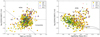 |
Fig. 2. Emission line diagnostic diagrams. Left panel: KEx and the right panel the MEx diagram. The circles, squares, crosses, and triangles represent pre-selected AGNs according to the methods of L04, S05, Ch17, and M12, respectively. The regions in both diagrams that are marked with dashed lines show the location of AGNs, composites, and star-forming galaxies. |
The demarcation lines used in the MEx diagram (Juneau et al. 2014) are the following:
 (6)
(6)
where y ≡ log([O III]l/Hβ) and x ≡ log(M⋆), and the coefficients are

Similarly, the lower curve is given by
 (7)
(7)
The coefficients are

We quote in Tables 2 and 3 the percentage of AGNs and composite and star-forming galaxies according to the methods proposed by L04, Ch17, S05, and M12, using the KEx and MEx diagrams, respectively. The final numbers of pure AGNs for the different selecting criteria of L04, Ch17, S05, and M12 are 132, 36, 113, and 54 objects using the KEx diagram and 101, 33, 67, and 63 objects using the MEx diagram.
Percentage of AGNs and composite and star-forming galaxies selected using the MIR and near-IR methods according to the KEx criteria (Zhang & Hao 2018).
Percentage of AGNs and composite and star-forming galaxies selected using the MIR and near-IR methods according to the MEx criteria (Juneau et al. 2014).
Figure 3 shows the Venn diagrams for the selected AGNs using the KEx and MEx diagrams according to the different selection methods in MIR and near-IR. The methods with the highest overlap are those of Ch17 and M12.
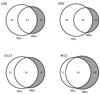 |
Fig. 3. Venn diagrams showing the number and overlap for pre-selected AGNs according to the L04, S05, Ch17, and M12 methods and also selected using the KEx and MEx diagrams. The area and overlap of each circle are proportional to the total number of each sample. Areas that represent AGNs that were only identified according to the MEx diagram are shown in grey. |
In Fig. 4 we show the spectroscopic redshift distribution for these AGNs selected following the different MIR and near-IR methods using the KEx (left panel) and MEx (right panel) diagrams. The S05 method preferably selects AGNs at lower redshifts (z < 0.5), according to the KEx and MEx diagrams. Up to z = 0.9, the remaining MIR and near-IR methods select a similar fraction of AGNs.
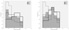 |
Fig. 4. Spectroscopic redshift distribution for AGNs selected according the different MIR and near-IR methods using the KEx (left panel) and MEx (right panel) diagrams. Dotted and shaded histograms represent the distributions using the methods proposed by S05 and L04, and solid and dashed line histograms show the methods proposed by M12 and Ch17, respectively. |
5. X-ray, near-UV, optical and mid- and near-IR properties
5.1. X-ray emission
We carried out an analysis of the X-ray emission of the pre-selected AGN sample using MIR and near-IR methods. We cross-correlated our pre-selected AGN catalogues with the X-ray catalogue presented by Civano et al. (2016). This catalogue is the COSMOS-Legacy Survey, a 4.6 Ms Chandra program on the 2.2 deg2 of the COSMOS field. in Table 4 we present the number of X-ray sources detected according to the MIR and near-IR methods of L04, Ch17, S05, and M12. We found 14%, 40%, 13%, and 38% of the sources with X-ray emission according to the pre-selection methods in the MIR and near-IR of L04, Ch17, S05, and M12, respectively.
Number of AGN candidates with X-ray emission according to the MIR and near-IR methods of L04, Ch17, S05, and M12.
In Fig. 5 we plot the distribution of pre-selected AGNs with X-ray emission using the KEx (left panel) and MEx (right panel) diagrams. The success rate of the mid-IR/near-IR methods in finding objects with X-ray emission without making any luminosity cut is somewhat lower than the AGN percentage obtained by either the KEx or MEx method.
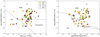 |
Fig. 5. Sources detected with X-ray emission for AGNs pre-selected according the different MIR and near-IR methods using the KEx (left panel) and MEx (right panel) diagrams. |
This may be due to the fact that there are many obscured AGNs in our sample whose X-ray emission is blocked by a large amount of dust (e.g., Compton-thick AGNs). Although it is also known that a high percentage of X-ray sources is located outside the selection criteria in the MIR (e.g., for the S05 criteria, see e.g., Mendez et al. 2013). The percentages of AGNs, composites, and SFs with X-ray emission for each MIR and near-IR method can be found in Tables 5 and 6 using the KEx and MEx diagrams.
Percentage of AGNs and composites and star-forming galaxies with X-ray emission selected using MIR and near-IR methods according to the KEx criteria.
Percentage of AGNs and composites and star-forming galaxies with X-ray emission selected using MIR and near-IR methods according to the MEx criteria.
In Fig. 6 we plot the Venn diagrams for the selected AGNs using the KEx and MEx diagrams with X-ray emission, according to the different selection methods in MIR and near-IR. Only a low percentage of sources overlap between the different MIR methods using the KEx and MEx diagnostic diagrams. The MIR methods with the greatest success in selecting X-ray AGNs are those of L04 and S05 (∼79%) using the MEx line diagnostic diagram. When no distinction is made between the pre-selected AGNs using MIR and near-IR methods, the MEx diagram presents a higher success rate to select AGNs with X-ray emission (76%) than those selected using the KEx diagram (71.7%).
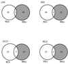 |
Fig. 6. Venn diagrams showing AGNs with X-ray emission according to the L04, S05, Ch17, and M12 methods and also selected using the KEx and MEx diagrams. |
5.2. Stellar mass and Ks-band absolute magnitude
In order to study the photometric properties of the MIR and near-IR selected AGNs, we analysed the stellar mass and the Ks-band absolute magnitude properties. We used the MASS_BEST estimator from the COSMOS2015 catalogue, which is estimated using the SED fitting techniques (Laigle et al. 2016). Figure 7 shows these two parameters for AGNs selected using the KEx and MEx diagrams in the left and right panels, respectively. In each of the plots we included AGNs pre-selected using the MIR and near-IR methods of L04, S05, Ch17, and M12. In the left panel of Fig. 7, the AGNs selected according to the S05 method present a large fraction of low-luminosity and low-mass objects compared to the other methods. The horizontal lines in this panel show the stellar mass completeness obtained by Laigle et al. (2016) for the regions called 𝒜Deep (dotted lines) and 𝒜UD in the redshift range 0.35 < z < 0.65 and 0.65 < z < 0.95, respectively (see Table 6 in Laigle et al. 2016).
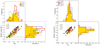 |
Fig. 7. AGN host stellar mass vs. absolute Ks-band magnitude using the KEx (left panel) and the MEx (right panel) line diagnostic methods. The horizontal dashed line shows the stellar mass completeness obtained by Laigle et al. (2016) for the regions called 𝒜Deep (dotted lines) and 𝒜UD in the redshift range 0.35 < z < 0.65 and 0.65 < z < 0.95, respectively. The upper and right panels in each figure show the absolute Ks band and the stellar mass distributions for each sample. Circles, squares, crosses, and triangles represent pre-selected AGNs according to the methods of S05, L04, Ch17, and M12, respectively. |
Some parameters may present bimodalities in their distributions. In order to test the existence of bimodality in the colour and/or mass distributions, we used two independent tests: a Gaussian mixture modelling (GMM), and the dip tests. The GMM statistics were first implemented by Muratov & Gnedin (2010). This code uses information from three different statistic tools: the kurtosis, the distance from the mean peaks (D), and the likelihood ratio test (LRT) in order to quantify the probability that the distributions are better described by a bimodal than a unimodal distribution. According to this code, the requirement for a distribution to be considered bimodal is to obtain a negative value for the kurtosis, the separation of the peaks, D, defined as  (where μx and σx are the mean and standard deviations of the two peaks of the proposed bimodal distribution), which is required to be greater than 2 and p(χ2) < 0.001, a p-value, which gives the probability of obtaining the same χ2 from a unimodal distribution. The dip test was originally proposed by Hartigan & Hartigan (1985), and unlike the GMM test, it has the benefit of being insensitive to the assumption of Gaussianity. The dip test measures multimodality based on the cumulative distribution of the input sample and is defined as the maximum distance between the cumulative input distribution and the best-fitting unimodal distribution. This test is similar to the Kolmogorov–Smirnov test, but the dip test searches specifically for a flat step in the cumulative distribution function, which corresponds to a dip in the histogram representation. The code was presented in Muratov & Gnedin (2010) and provides a parameter that represent the significance level at which a unimodal distribution can be rejected4.
For the sample of pre-selected AGNs, according to the S05 method and using the KEx diagram, we find bimodality in the MKs and stellar mass distributions, according to the following values obtained using the GMM code: kurtosis = − 1.01, μ1 = −20.71 ± 0.13, μ2 = −22.70 ± 0.32, D = 3.0 ± 0.5 and p(χ2) < 0.001 for the MKs distribution and kurtosis = − 1.02, μ1 = 9.50 ± 0.10, μ2 = 10.75 ± 0.15, D = 3.8 ± 0.4 and p(χ2) < 0.001 for the stellar mass distribution. Using the dip code, we find p = 0.78 and p = 0.83 for the MKs and stellar mass distributions, respectively. In both cases, we did not include any sources below the stellar mass limit according to Laigle et al. (2016). For the remaining objects selected from the KEx diagram and according to the methods of L04, Ch17, and M12, the two codes did not yield values corresponding to bimodal distributions for stellar mass and MKs values, while the stellar mass and MKs distributions for AGNs obtained according to the MEx diagram (Fig. 7, right panel) are not bimodal for all samples of MIR and near-IR selected AGNs, according to the GMM test.
5.3. Quiescent and star-forming galaxy samples
Williams et al. (2009) employed a rest-frame colour–colour selection technique using purely photometric data to identify samples of quiescent and star-forming galaxies at redshifts z ≲ 2. The quiescent samples tend to be early-type galaxies forming a different red sequence in the colour–colour observed in the UVJ diagram. Many authors have used this diagram to separate populations of predominantly blue colour star-forming galaxies from red and quiescent galaxies using a variety of rest-frame colours with similar filters (Patel et al. 2011; Arnouts et al. 2013; Ilbert et al. 2013; Straatman et al. 2016; Fang et al. 2018).
Figure 8 shows the rest-frame MNUV − Mr vs. Mr − MJ colour–colour diagrams for AGNs pre-selected using the L04, S05, Ch12, and M12 methods for AGNs obtained from KEx and MEx diagrams (left and right panels, respectively). The dashed lines represent the boundaries that separate regions occupied by quiescent and star-forming galaxies taken from Ilbert et al. (2013). In each figure, we also included the corresponding colour distributions for each MIR and near-IR methods (upper and right panels). We also included a sample of galaxies taken from zCOSMOS-good with 0.3 ≤ zsp ≤ 0.9 and without any pre-selected AGNs according to L04, S05, Ch17, and M12 methods (grey dots and dotted histograms). Hereafter we call this sample zCOSMOS non-AGN.
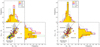 |
Fig. 8. Rest-frame (MNUV − Mr) vs. (Mr − MJ) colour–colour diagram for AGN host galaxies selected according to the KEx (left panel) and the MEx (right panel) line diagnostic methods. Dashed lines mark regions that separate quiescent (upper left corner) and star-forming galaxies. The symbols are the same as in Fig. 7. The zCOSMOS non-AGN sample, a comparison sample of galaxies with a similar mass distribution at 0.3 ≤ zsp ≤ 0.9, is represented by grey points. Colour distributions are included in the upper and right panels. The comparison sample is represented by dotted grey circles. |
Spitler et al. (2014) studied the high-redshift massive galaxy population in the ZFOURGE survey. They used an U − V vs. V − J colour–colour diagram in order to analyse the quiescent and star-forming galaxy populations. They split the star-forming sample into two groups: one with high dust content (V − J > 1.2), and the other with low dust content (V − J < 1.2). We used this separation criterion to transform the colours V − J into R − J through the linear relation found between the two colours using our zCOSMOS-good sample,

The majority of the AGNs selected by the IR methods are located within the locus where the star-forming galaxies reside. The S05 sample presents a considerable fraction of blue objects located in the region populated by SF galaxies with low dust content in both MNUV − Mr and Mr − MJ colours for the sample of AGNs selected according to the KEx diagram. On the other hand, AGNs selected according to the MEx diagram do not present a locus of objects in the area occupied by low dust content star-forming galaxies as observed in the KEx diagram. This excess of sources with low dust content observed in the methods of L04 and S05 according to the KEx diagram is shown by the large number of objects that do not present overlap, as we showed in Fig. 3.
Without distinguishing between AGNs that were pre-selected using MIR and near-IR methods, we find that only 5.4% and 11.5% of AGNs are located in the quiescent region according to the KEx and MEx diagrams, respectively. Within the observed bimodality in galaxy colours, some authors affirmed that there would be a transition population between the red and blue populations, the so-called the green valley galaxies (Wyder et al. 2007; Salim et al. 2007; Salim 2014). This region is thought to represent a transition in the life of galaxies ranging from blue galaxies with high star formation rates to passive galaxies with predominantly red colours (Salim et al. 2007; Salim 2014). According to some authors, the limit values that define this region are between 3 < MNUV − Mr < 5 (Salim et al. 2007), 3.5 < MNUV − Mr < 4.5 (Salim et al. 2009), or 3.2 < MNUV − Mr < 4.1 (Mendez et al. 2011) for galaxies at 0.4 < z < 1.2, which coincides for a sample of galaxies at low redshifts studied by Coenda et al. (2018) with similar host stellar masses. In the left panel of Fig. 8, we find that the colours of the AGN samples selected using the KEx diagram are located mostly in the blue branch of the colour–colour diagram, while the sample of AGNs selected using the MEx diagram are located near the green valley, although with slightly bluer colours than the average position of green valley galaxies.
The colour distribution for the zCOSMOS non-AGN sample shows a clear bimodality. using the GMM code, we found the following values: kurtosis = −0.888, μ1 = 1.9 ± 0.03, μ2 = 4.60 ± 0.06, D = 3.43 ± 0.11, and p(χ2) < 0.001, while using the dip test, we found p = 1.0. For the sample of AGNs selected using the KEx diagram, we find that the Mr − MJ colour distributions according to the Ch17 and M12 are not bimodal, while the corresponding colour distribution of S05 is bimodal according to the GMM and dip codes. We obtained the following values using the GMM code: kurtosis = − 0.68, μ1 = 0.35 ± 0.05, μ2 = 0.92 ± 0.10, D = 3.0 ± 0.6, p(χ2) < 0.001, and p = 0.9. The sample of L04 presents a moderate bimodality according to the p-value p(χ2) = 0.22 and p = 0.15 using the GMM and dip codes, respectively. For the MNUV − Mr colour distribution, the results obtained with the GMM code shows that the S05 method is not bimodal, while the M12 and Ch17 methods present a moderately bimodality (p(χ2) = 0.117 and 0.09, and p = 0.31 and p = 0.1, using the GMM and dip tests, respectively), and the L04 method presents a bimodal colour distribution with the following values: kurtosis = − 0.68, μ1 = 1.43 ± 0.10, μ2 = 2.9 ± 0.15, D = 2.3 ± 0.3, and p(χ2) < 0.001 using the GMM code. Using the dip test, we obtained p = 0.76. For the case of the AGNs selected using the MEx diagram (right panel of the Fig. 8), all colour distributions are well represented by unimodal distributions. For the Mr − MJ colours, the distributions are well characterised with μ = 0.91 ± 0.01 and σ = 0.28 ± 0.04, while for the MNUV − Mr colour distribution, we find μ = 3.0 ± 0.1 and σ = 0.83 ± 0.03.
5.4. AGN MIR colour–colour diagram
In this section we study the MIR IRAC four-colour position of each AGN according to the MIR and near-IR methods. In Fig. 9 we plot the MIR colour–colour diagrams for pre-selected AGNs according to the methods of L04 and Ch17 (small dots). We also include in the same plot the corresponding [4.5]−[8.0] and [3.6]−[5.8] AGN candidate colours using the methods of S05 (squares) and M12 (pentagons). The region marked with dashed and dot-dashed lines show the selection criteria of L04 and Ch17, respectively. Horizontal dotted lines show the correction of +0.25 magnitudes proposed by Lacy et al. (2007). These authors presented a small modification to the AGN selection box, moving the log(S5.8/S3.6) cut by +0.1 compared to Lacy et al. (2004) in order to remove possible non-AGN contaminants. As these authors claimed, the exact position of this cut is not critical and the line diagnostics made through KEx and MEx diagrams eliminate other possible contaminants. We calculated the percentages of AGNs, composites, and SF galaxies of the objects within the rectangle defined by the difference between the selection boxes of L04 and L07 (see Fig. 9). According to the KEx diagram, we find (AGNs, composites, and SF) = (30,48,22)% and using the MEx diagram (AGNs, composites, and SFs) = (19,16,65)%. We find that the percentages of the different galaxy types are similar to those found by L04 (see Tables 1 and 2). We therefore use the criterion of L04 instead of the criterion presented in Lacy et al. (2007). We also plot a solid line that represents the power-law locus, that is, the line on which a source with a perfect power-law SED would fall. Filled circles along this line denote power-law slopes from α = −0.5 (lower left) to α = −3.0 (upper right). Some dots corresponding to the S05 criterion fall outside the L04 and Ch17 boxes. These have bluer colours in both [3.6]−[5.8] [4.5]−[8.0] and are faint in the Ks-band on average compared to the remaining MIR and near-IR methods. These sources seem to continue the power law towards positive values of α. As stated in Barmby et al. (2006), AGN-dominated objects would have red power laws with α < 0 (preferentially with α < −0.5; Donley et al. 2007, 2008), while star-dominated galaxies would have blue SEDs with α ∼ +2. This evidence together with the results in Figs. 7 and 8 indicates that some of the objects selected according to the method proposed by S05 represent low-mass faint star-forming (with a possible weak AGN component) galaxies at lower redshifts.
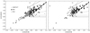 |
Fig. 9. Mid-IR ([4.5]−[8.0] vs. [3.6]−[5.8]) colour–colour diagrams for AGNs selected according the methods present by L04 and Ch17 (small dots). We also included the AGN colours using the methods present by S05 (squares) and M12 (pentagons). The region marked with dashed and dot-dashed lines show the selection criteria of L04 and Ch17, respectively. Horizontal dotted lines shows a correction of +0.25 magnitudes proposed by Lacy et al. (2007). The line with filled black circles indicates the locus of sources whose spectrum can be described as a power law with α = −0.5 (lower left) to α = −3.0 (upper right). |
6. Properties of AGNs selected by KEx and MEx diagnostic diagrams
In this section we study the AGN properties according to the KEx and MEx diagrams without distinguishing between the pre-selected AGNs using MIR and near-IR methods. In Fig. 10 we show the KEx and MEx diagrams for the sample of MIR and near-IR pre-selected AGNs using the methods of L04, S05, Ch17, and M12. The vertical bar indicates the [O III] luminosity values for each AGN. We calculated the [O III] luminosity using the standard formula
![Mathematical equation: $$ \begin{aligned} L_{[\mathrm {O}\,{\small{\text{III}}} ]}=\frac{4\pi d^2_{\rm L}}{(1+z)}f_{[\mathrm {O}\,{\small{\text{III}}}]} ,\end{aligned} $$](/articles/aa/full_html/2022/08/aa42228-21/aa42228-21-eq12.gif) (8)
(8)
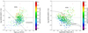 |
Fig. 10. Kinematics (left panel) and mass-excitation (right panel) diagrams for sources selected according to MIR and near-IR methods proposed by S05, L04, Ch17, and M12. The vertical bar represents the [O III] λ5007 luminosity of each source. The horizontal dotted line in the right panel shows the limit at y = 0.3 that separate AGNs in the KEx diagram. |
where dL is the luminosity distance, and f[O III] is the [O III] λ5007 line flux.
Due to the redshift range of the AGN sample and the spectral coverage 5550–9450 Å of the VIMOS data that we used, we did not correct the [O III] λ5007 flux to account for the absorption due the narrow-line region itself (see e.g., Maiolino et al. 1998; Bassani et al. 1999; Vignali et al. 2006, 2010; Panessa et al. 2006; Lamastra et al. 2009). This reddening correction uses the Hα/Hβ Balmer decrement, and we have only Hα emission up to z ∼ 0.4.
Objects in the KEx diagram (left panel of Fig. 10) that are located in the area in which AGNs reside have higher [O III] luminosities than objects that are located in areas populated by star-forming and composite galaxies. In the right panel of Fig. 10, we plot the MEx diagram for AGNs pre-selected in the MIR and near-IR wavelengths. We also included a horizontal line at log([O III]/Hβ) = 0.3 that represents the limit for the vast majority of AGNs selected using the KEx diagram. According to this diagram, we find that the objects located in the region populated by star-forming galaxies around the coordinate (log(Stellar mass), log([O III]/Hβ)) = (9.4, 0.6) also have higher [O III] luminosities than those found in the AGN sample. The [O III] emission in AGNs might come from the narrow-line region, but also from the HII regions of SF galaxies. As postulated by Zhang & Hao (2018), the [O III] emission from AGNs traces the bulge kinematics, while in star-forming galaxies, it comes from HII regions located in the disk.
In order to establish whether these objects are AGNs as determined by the KEx diagram or star-forming galaxies with high [O III] luminosities according to the MEx diagram, we used a sample of star-forming galaxies with extreme emission lines taken from Amorín et al. (2015). These authors studied a sample of 183 extreme emission-line galaxies (EELGs) at redshift 0.11 ≲ z ≲ 0.93 selected from the 20k zCOSMOS survey with unusually large emission line equivalent widths and high specific star formation rates. These objects were identified with compact, low-mass, low-metallicity, vigorously star-forming systems associated with luminous and higher-z counterparts of nearby HII galaxies and blue compact dwarfs. In order to elucidate this difference, we plot in Fig. 11 the KEx (left panel) and MEx (right panel) diagrams for a sample of star-forming galaxies with extreme emission lines with 0.3 ≤ zsp ≤ 0.9 taken from Amorín et al. (2015). For the case of the KEx diagram, we measured the width of the [O III] λ5007 emission line (σ[O III]) as described in Sect. 3. The vertical bar represents the [O III] luminosities with the same scale as in Fig. 10. The right panel of Fig. 11 shows that all these SF galaxies have log([O III]/Hβ) > 0.3 and high [O III] luminosity values, some even higher than observed for AGNs in Fig. 10. All SF forming galaxies selected in the Amorín et al. (2015) catalogue are located within the boundaries of the SF galaxies according to the MEx diagram. However, the same sample of SF galaxies is found within the region populated by AGNs according to the KEx method. This shows that the width of OIII used in the KEx diagram does not allow a clear separation between the emission of the [O III] λ5007 lines coming from the AGN from that originating in the HII regions of galaxies with high star formation rates.
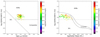 |
Fig. 11. Kinematics (left panel) and mass-excitation (right panel) diagrams for extreme emission line star-forming galaxies taken from Amorín et al. (2015). The vertical bar represents the [O III] λ5007 luminosity of the sources. The horizontal dotted line in the right panel shows the limit at y = 0.3 that separates AGNs in the kinematics-excitation diagram. |
7. X-ray emission, black hole mass, and morphology of the AGNs selected through the MEx diagram
We have shown that the KEx diagram presents great contamination by SF galaxies within the limits that demarcate the selection of AGNs. In this section, we analyse the AGN properties selected only according to the MEx diagram.
7.1. AGN X-ray emission properties
We investigate here the X-ray properties of AGNs. The hardness ratio (HR) is an indication of the spectral shape and can be used to separate obscured and unobscured AGNs in the X-ray wavelengths. For this reason, we use the HR measurements from the catalogue of Civano et al. (2016), which is defined as
 (9)
(9)
where H and S are the count rates in the hard and soft bands, respectively.
In Fig. 12 we plot the HR as a function of rest-frame hard X-ray luminosity for each MIR and near-IR method using the MEx diagram, which is calculated as
 (10)
(10)
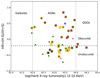 |
Fig. 12. Hardness ratio as a function of hard (2–10 keV) X-ray luminosity. Vertical dashed lines show the typical separation for normal galaxies, AGNs, and quasars used in the X-rays. The symbols are the same as in Fig. 4. |
where dL is the luminosity distance (cm), fX is the X-ray flux (erg s−1 cm−2) in the hard band, and the photon index was assumed to be Γ = 1.8 (Tozzi et al. 2006).
The dashed horizontal line shows the HR value (HR = −0.2) for a source with a neutral hydrogen column density, NH > 1022 cm2 (Civano et al. 2012), which is used by several authors (Gilli et al. 2009; Treister et al. 2009; Marchesi et al. 2016) to separate obscured and unobscured sources in the X-rays at all redshifts. Vertical dashed lines show the typical separations used in the X-rays following Treister et al. (2009) for normal galaxies (LX < 1042 erg s−1), AGNs (1042 < LX < 1044 erg s−1) and quasars (LX > 1044 erg s−1).
For each MIR and near-IR method, we find the percentage of obscured (HR > −0.2) sources of 52, 54, 65, and 71% according to the methods proposed by L04, Ch17, S05, and M12, respectively. Without distinguishing between AGNs pre-selected using MIR and near-IR methods, we find 59.13% and 40.87% of obscured and unobscured AGNs, respectively. We also performed the same calculations for the sample of X-ray sources taken from Civano et al. (2016) with 0.3 ≤ zsp ≤ 0.9. In this sample, we find very similar results of obscured (50.6%) and unobscured (49.4%) sources. By comparison, we found that our AGN samples selected according the S05 and M12 methods, also identified in the MEx diagram, have 15–21% excess of obscured objects (HR > −0.2).
7.2. Black hole and AGN accreting properties
In this section we study the black hole mass and accretion properties of AGNs selected using different diagnostic diagrams. We estimated the black hole mass of AGNs from the width of the [O III] λ5007, following the relation presented in Nelson (2000),
![Mathematical equation: $$ \begin{aligned} \log (M_{\rm BH})=(3.7\pm 0.7)\times \mathrm {log}(\sigma _{\rm [\mathrm{O}\,{\small {\text{III}}} ]})-(0.5\pm 0.1) ,\end{aligned} $$](/articles/aa/full_html/2022/08/aa42228-21/aa42228-21-eq15.gif) (11)
(11)
where the MBH, the black hole mass, is in units of M⊙ and σ[O III] (calculated as FWHM[O III]/2.35) in km s−1. These authors used the stellar velocity dispersion σ⋆ or σ[O III] in an equivalent way due to their assumption that for most AGNs the forbidden line kinematics are dominated by virial motion in the host galaxy bulge.
This evidence is based on the results obtained by Nelson & Whittle (1996), who found a moderately strong correlation between FWHM[O III] and σ⋆ for the majority of Seyfert galaxies, indicating roughly equal absorption and emission-line widths. Following these premises, we plot in Fig. 13 the black hole mass distributions for AGNs selected using the MEx diagram according to the MIR and near-IR methods of L04, S05, Ch17, and M12. AGNs selected using the MEx diagram show similar log(BH mass) distributions for all AGNs selected in the MIR and near-IR wavelengths. We also included the cumulative fraction distributions for each of the MIR and near-IR methods (top left panel), in order to highlight the differences between the distributions.
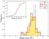 |
Fig. 13. Distributions of black hole mass for each MIR and near-IR method using the MEx diagram. The inset box represents the cumulative fraction distribution of the MIR and near-IR methods. |
Figure 14 shows grey contours representing the [O III] λ5007 luminosity vs. black hole mass for AGNs selected using the MEx line diagnostic diagrams. Dashed line contours are data taken from highly accreting QSOs selected from the SDSS DR7 survey from Negrete et al. (2018). Dotted lines from upper to lower right indicate ∼100%, ∼10%, and ∼1% of the Eddington limit, respectively, assuming bolometric correction of 3500 for L[O III] (Heckman et al. 2004; Choi et al. 2009). These extreme accreting QSOs were selected according to the FWHM of the broad component (BC) of Hβ (HβBC) and the ratio of the equivalent width of Fe II and HβBC (specifically with RFeII > 1, Negrete et al. 2018). The peak of this distribution coincides with the line indicating sources with ∼10% of the Eddington limit. For the sample of AGNs identified using the MEx diagrams, the peak of the distribution is only above the line correspond for sources with ∼1% of the Eddington limit. In the figure, our AGN sample according to the MEx diagnostic diagrams have black hole mass distributions similar to those found in highly accreting QSOs at similar redshifts, although the [O III] λ5007 luminosity values are ∼0.7 dex lower on average than the highly accreting QSO sample.
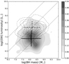 |
Fig. 14. OIII λ5007 luminosity vs. black hole mass for AGNs selected according to the MIR and near-IR methods using the MEx line diagnostic diagrams (grey contours). Dashed line contours represent the corresponding values for highly accreting QSOs. Point lines from upper to lower right indicate ∼100%, ∼10%, and ∼1% of the Eddington limit, respectively, assuming bolometric correction 3500 for OIII luminosity (Heckman et al. 2004; Choi et al. 2009). Solid and dashed line bars represent the mean and 1σ values for our sample of AGNs and for the sample of highly accreting QSOs, respectively. |
7.3. Morphology
An important tool in diagnostic galaxy evolution is the galaxy morphology. In this section we analyse the different AGN host morphology properties according to parametric methods, such as the Sérsic index and non-parametric statistics, such as the Gini coefficient and the asymmetry.
7.3.1. Sérsic index
Griffith et al. (2012) presented a photometric and morphological database using publicly available data obtained with the ACS instrument on board the Hubble Space Telescope, the Advanced Camera for Surveys General Catalog (ACS-GC). These authors calculated morphological parameters such as the Sérsic index (Sérsic 1963) using an automated fitting method called GALAPAGOS (Häußler et al. 2011), which is compound by the GALFIT (Peng et al. 2002) and SExtractor (Bertin & Arnouts 1996) codes. We cross-correlated our AGN sample with this catalogue using a matching radius of 1 arcsec. We found that 97% of our AGNs selected by the MEx diagram are presented in the catalogue. In Fig. 15 we plot the MIR colour–colour diagram for pre-selected AGNs according to the methods present by L04, S05, Ch17, and M12 for AGNs obtained using the MEx diagram. The region marked with dashed and dot-dashed lines show the selection criteria of L04 and Ch17, respectively. We included a relative grey scale showing the Sérsic index values of each source.
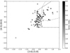 |
Fig. 15. MIR colour–colour diagrams for pre-selecting AGNs according the methods presented by L04, S05, Ch17, and M12 using the MEx line diagnostic diagram. The region marked with dashed and dot-dashed lines show the selection criteria of L04 and Ch17, respectively. The vertical bar shows the corresponding values for the Sérsic index. |
We restricted the Sérsic index to be in the range 0.2 < n < 8, and we divided the galaxies into three classes, according to Griffith & Stern (2010): sources with 0.2 < n < 1.5 comprised of late-types or spirals, those with 1.5 ≤ n ≤ 2.5 comprised of galaxies with blended morphologies with bulge+disk components, and with 2.5 < n < 8 generally comprised of ellipticals or early-type galaxies. We did not consider extreme Sérsic model profiles n = 0.2 and n = 8, which probably correspond to erroneous fits or systematics.
Griffith & Stern (2010) investigated the optical morphologies of AGN candidates identified at MIR, X-ray, and radio wavelengths. They defined six samples of AGNs called IRAC1, IRAC2, XMM1, XMM2, VLA1, and VLA2. The IRAC1 sample consists of the brighter MIR AGN candidates selected to the 5σ depth of the original IRAC Shallow Survey with MIR criteria proposed by Stern et al. (2005). The IRAC2 consists of a fainter sample of objects detected in all four IRAC bands down to the full 5σ depth of the Spitzer Deep Wide-Field Survey, but not already detected in the IRAC1 sample. The XMM1 sample consists of sources with soft (0.5–2.0 keV) X-ray fluxes S0.5 − 2.0 = 5.0 × 10⁻¹⁵ erg cm−2 s−1 and the fainter sample, XMM2, of sources with S0.5 − 2.0 < 5.0 × 10⁻¹⁵ erg cm−2 s−1. The radio VLA1 (Very Large Array 1) consists of brighter sources, with flux densities greater than or equal to 1 mJy (S1.4 ≥ 1.0 mJy) and VLA2, of fainter sources, with flux densities within 0.3 ≤ S1.4 < 1.0 mJy. We also constructed a sub-sample of AGNs that we call G10z, obtained from the Griffith & Stern (2010) catalogue using the same redshift cuts (0.3 ≤ zph ≤ 0.9, estimated using photometric redshifts) as our AGN samples.
Table 7 shows the percentage of sources found according to their Sérsic index values separated into three classes using the MEx diagram, the bright and faint samples obtained with IRAC, XMM, and VLA, and the G10z sample. Comparing our n values with other MIR, X-ray, and radio selected AGNs, we find that AGNs selected in the fashion of MEx diagram have similar percentages of late types or spirals (with 0.2 < n < 1.5), spiral/late-type galaxies with bulge+disk components (with 1.5 ≤ n ≤ 2.5), and galaxies with blended morphologies with bulge+disk components with 2.5 < n < 8 as the IRAC1 and IRAC2 selection methods. We also find similar percentages between our AGNs for the three classifications according to the Sérsic index values and the G10z sample with similar redshift distributions, although the sample of weak and bright sources detected in radio wavelengths (VLA1 and VLA2) presents a higher percentage of objects with early-type morphologies than the sample of AGNs according to the MEx diagram.
Percentage of sources found according to Sérsic index values, separated into three classes using the MEx diagram, and IRAC1, IRAC2, XMM1, XMM2, VLA1 and VLA2 samples from Griffith & Stern (2010).
7.3.2. Gini coefficient and asymmetry index
Non-parametric approaches to quantitative morphology have been developed over the last years by several authors (Abraham et al. 1996; Conselice 2003; Lotz et al. 2004, 2008; Cassata et al. 2007; Tasca et al. 2009). Conselice (2003) presented the CAS parameters: the concentration index, the asymmetry, and clumpiness. The asymmetry parameter A quantifies the degree to which the light of a galaxy is rotationally symmetric. The value of A is calculated by rotating a galaxy through 180° and subtracting this rotated galaxy from the original and comparing the absolute value of the residuals of this subtraction to the original galaxy flux (Conselice et al. 2000). Zero a symmetry would correspond to a completely symmetric galaxy, typically of elliptical types with smooth light profiles, and asymmetry = 1 would correspond to a totally asymmetric one, such as spiral galaxies, irregular types, or galaxies with major merger signatures.
Other parameters were later added, such as the Gini coefficient and the M20 parameter (Lotz et al. 2004, 2008). The Gini coefficient, first introduced by Abraham et al. (2003), is a statistical tool originally used in economics for measuring the distribution of wealth within a population, and was found useful in astrophysics to determine the quantitative measurement of inequality of galaxy light distribution between pixels. Gini = 1 would mean that all the light is in one pixel, while Gini = 0 would mean that every pixel has an equal share. The Gini coefficient is a good marker of an overall smoothness, and therefore it can be a good probe of a merger process in general.
The morphological measures we used were obtained from the catalogue presented by Cassata et al. (2007), which provides information of non-parametric diagnostics of galaxy structure using the Hubble Space Telescope ACS for 232 022 galaxies up to F814W = 25 mag. In Fig. 16 we plot the Asymmetry vs. the Gini coefficient for AGNs selected using the MEx diagnostic diagram. The horizontal dashed lines at log(asymmetry) < − 0.46 (Conselice 2003) shows the dividing line above which objects are expected to be major mergers. The vertical dotted line at log(Gini) < − 0.3 (Abraham et al. 2007) separates early-type galaxies to the right. Dashed line contours in the figure represent the morphological values observed for galaxies in the zCOSMOS-non-AGN sample.
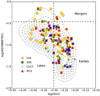 |
Fig. 16. log(asymmetry) vs. log(Gini) coefficient for AGNs selected using the MEx method. Symbols are the same as in the other figures. Dashed lines show the regions populated by mergers and late- and early-types galaxies. Dashed line contours represent galaxies taken from the zCOSMOS-non-AGN identified in the Cassata et al. (2007) catalogue. |
A visual inspection performed of AGNs using the ACS F814W images shows that spiral galaxies preferentially lie in the low-Gini low-asymmetry region of Fig. 16, although many spiral galaxies with predominant bulges also occupy the region established for early types. This result agrees with some works that showed that late-type galaxies occupy a large scattered zone to the left and right (occupied by early types) of the line log(Gini) < − 0.3 (Abraham et al. 2007; Kartaltepe et al. 2010). Despite this, AGNs denominate the area populated by late-types to that defined by log(asymmetry) < − 0.46 and log(Gini) < − 0.3.
Without distinguishing between AGNs that were pre-selected using the MIR and near-IR methods, we find the following percentages: (early, late, and merger) = (67.5, 23.2, and 9.3)%. For the sample of control galaxies zCOSMOS non-AGN, we find (early, late, and merger) = (44.3, 49.7, and 6)%. The percentage of late-type galaxies in the MEx AGN sample is lower than a half when compared to the control sample of galaxies without AGNs. On the other hand, the percentages of early types and mergers are one and a half times as high as in the control sample.
8. Summary and discussions
We have studied four selection methods in the MIR and near-IR wavelengths: the IRAC colour–colour cuts proposed by Lacy et al. (2004) and Stern et al. (2005), according to a power-law emission (Chang et al. 2017) and a combination of MIR and near-IR emission and based on the predictions by galaxy and AGN templates (Messias et al. 2012). We employed the line diagnostic diagrams that use the [O III]/Hβ line ratio and the [O III]l line width, the kinematic-excitation diagram (Zhang & Hao 2018), stellar mass, and the mass-excitation diagram (Juneau et al. 2011, 2014). The main results are summarised below:
Of the four MIR and near-IR methods we analysed, two (L04 and S05) have high contamination by SF and composite galaxies: between 60 and 70% of contamination of SF according to the MEx diagnostic diagram and ∼50% of composite galaxies according to KEx diagram. These methods were also reported by other authors as contaminated by SF galaxies (Sajina et al. 2005; Donley et al. 2012; Mendez et al. 2013; Kirkpatrick et al. 2013).
The methods with the greatest success in selecting AGNs, according to the diagnostic diagrams, are those presented by M12 and Ch17, with a success rate ranging from 48 to 56%. The method proposed by M12 selects a large number of AGNs (63 according to the MEX method) and appears to be reasonably efficient in the success rate (61%) and total number of AGN recovered. These results agree with those found by Messias et al. (2012), who determined with the help of colour tracks for various galaxy type models that the contamination by normal galaxies appears to be significantly reduced in comparison to L04 and S05 methods.
We find that the S05 method selects a considerable percentage of predominantly blue, low-mass, and low redshift objects with MIR spectra that follow positive blue slopes (α ≥ 0). These are characteristic of star-dominated sources at low redshifts, which generally exhibit positive IRAC power-law emission following the Rayleigh-Jeans tail of the black-body spectrum (Park et al. 2010). This effect is greater when AGNs are selected according to the KEx method compared to the MEx method, which when using stellar masses, allows a better distinction between low-mass galaxies with high star formation from pure AGNs.
By analysing the colours in the near-UV and optical (MNUV − Mr) and according to the KEx diagram, the method proposed by S05 selects a high fraction of objects identified with SF galaxies with low dust content.
According to the KEx and MEx diagrams, the MNUV − Mr colour distributions of most AGNs are bluer than those found for the green valley galaxies, which is more noticeable in the KEx diagram. Similar results were found by Hickox et al. (2009) in a sample of IRAC-selected AGNs using optical colours. These authors found that IRAC-selected AGNs are found throughout the galaxy colour–magnitude space, with a few hosts on the red sequence and a predominant population towards blue colours with respect to the green valley.
With respect to the KEx and MEx line diagnostic diagrams, from the analysis of the [O III] λ5007 luminosity and the MNUV − Mr colour, we find that the KEx diagram, which uses the width of the [O III] λ5007 line, probably does not allow a clear separation between the emission of the [O III] lines coming from an AGN from that originating in the HII regions of galaxies with high star formation rates. As noted by Zhang & Hao (2018), the explanation for the KEx method would consist of assuming that the width of the [O III] λ5007 line correlates with the stellar velocity dispersion (σ⋆). This would be correlated with the mass of the bulge and the stellar mass of the galaxy. Although several works have postulated the correlation between [O III] λ5007 and σ⋆ (Nelson 2000; Ho 2009; Komossa & Xu 2007), some works did not find this close correlation (Boroson 2003; Botte et al. 2005; Bennert et al. 2018; Sexton et al. 2019). Particularly, Botte et al. (2005) found that the width of the [O III] λ5007 line typically overestimates the stellar velocity dispersion. Therefore, the width of the [O III] λ5007 line would not be a good indicator to separate SF galaxies from pure AGNs.
According to the pre-selection methods in the MIR and near-IR of L04, S05, Ch17, and M12, we find that between 15% and 40% of objects have X-ray emission. Comparing the results obtained in a sub-sample of sources with 0.3 < z < 0.9 and X-ray emission in Civano et al. (2016), we found that the AGN samples according to the S05 and M12 methods (also identified according to the MEx diagram) have an excess of between 15 and 21% of obscured objects (HR > −0.2).
AGNs selected using MIR and near-IR methods according to the MEx diagrams have black holes with masses similar to highly accreting QSOs at similar redshifts, but are ∼0.7 dex less luminous in [O III] λ5007 luminosity.
The majority of hosts of AGNs identified using MEx diagrams are early-type galaxies. When compared to a suitable control sample with non-AGN galaxies with similar stellar mass and redshift distributions, we find that MEx-selected AGNs are 50% more probably found in early types and in galaxies with major merger signatures.
Studies of large samples of galaxies with AGNs are important to unravel the mechanisms of galaxy formation and evolution. To develop such studies we must discover what types of sources are identified by all various AGN selection techniques. In the last years several techniques were developed for the selection of AGNs in the IR wavelengths. In this work we find that a combination of criteria in the MIR and/or near-IR together with the use of line diagnostic diagrams that use the galaxy stellar mass offer a very good selection criteria for AGNs without contaminants such as normal galaxies or with high star-formation rates. These results will be used in future studies to analyse the environments and properties of different samples of AGNs.
The catalogue can be downloaded from ftp://ftp.iap.fr/pub/from_users/hjmcc/COSMOS2015/
Magnitudes presented in Stern et al. (2005) are referred to the Vega system and they were converted to the AB system using the relations taken from Zhu et al. (2011): ([3.6], [4.5], [5.8], [8.0])AB = ([3.6], [4.5], [5.8], [8.0])Vega + (2.79, 3.26, 3.73, 4.40).
IRAF (Image Reduction and Analysis Facility, Tody 1993) is distributed by the National Optical Astronomy Observatories, which is operated by the Association of Universities for Research in Astronomy (AURA) under cooperative agreement with the National Science Foundation (NSF).
Both GMM and dip test codes can be download from http://www-personal.umich.edu/~ognedin/gmm/
Acknowledgments
We thank the anonymous referee for his/her useful comments and suggestions. This work was partially supported by the Consejo Nacional de Investigaciones Científicas y Técnicas (CONICET) and the Secretaría de Ciencia y Tecnología de la Universidad Nacional de Córdoba (SeCyT). Based on data products from observations made with ESO Telescopes at the La Silla Paranal Observatory under ESO programme ID 179.A-2005 and on data products produced by TERAPIX and the Cambridge Astronomy Survey Unit on behalf of the UltraVISTA consortium. Based on zCOSMOS observations carried out using the Very Large Telescope at the ESO Paranal Observatory under Programme ID: LP175.A-0839 (zCOSMOS). This research has made use of the VizieR catalogue access tool, CDS, Strasbourg, France (DOI: 10.26093/cds/vizier). The original description of the VizieR service was published in 2000, A&AS 143, 23.
References
- Abraham, R. G., Tanvir, N. R., Santiago, B. X., et al. 1996, MNRAS, 279, L47 [Google Scholar]
- Abraham, R. G., van den Bergh, S., & Nair, P. 2003, ApJ, 588, 218 [NASA ADS] [CrossRef] [Google Scholar]
- Abraham, R. G., Nair, P., McCarthy, P. J., et al. 2007, ApJ, 669, 184 [NASA ADS] [CrossRef] [Google Scholar]
- Alarcon, A., Gaztanaga, E., Eriksen, M., et al. 2021, MNRAS, 501, 6103 [NASA ADS] [CrossRef] [Google Scholar]
- Alonso-Herrero, A., Pérez-González, P. G., Alexander, D. M., et al. 2006, ApJ, 640, 167 [Google Scholar]
- Alonso-Herrero, A., Ramos Almeida, C., Mason, R., et al. 2011, ApJ, 736, 82 [NASA ADS] [CrossRef] [Google Scholar]
- Amorín, R., Pérez-Montero, E., Contini, T., et al. 2015, A&A, 578, A105 [NASA ADS] [CrossRef] [EDP Sciences] [Google Scholar]
- Antonucci, R. 1993, ARA&A, 31, 473 [Google Scholar]
- Arnouts, S., Le Floc’h, E., Chevallard, J., et al. 2013, A&A, 558, A67 [NASA ADS] [CrossRef] [EDP Sciences] [Google Scholar]
- Ashby, M. L. N., Willner, S. P., Fazio, G. G., et al. 2013, ApJ, 769, 80 [Google Scholar]
- Ashby, M. L. N., Willner, S. P., Fazio, G. G., et al. 2015, ApJS, 218, 33 [NASA ADS] [CrossRef] [Google Scholar]
- Assef, R. J., Kochanek, C. S., Ashby, M. L. N., et al. 2011, ApJ, 728, 56 [NASA ADS] [CrossRef] [Google Scholar]
- Assef, R. J., Stern, D., Noirot, G., et al. 2018, ApJS, 234, 23 [Google Scholar]
- Audibert, A., Riffel, R., Sales, D. A., Pastoriza, M. G., & Ruschel-Dutra, D. 2017, MNRAS, 464, 2139 [NASA ADS] [CrossRef] [Google Scholar]
- Baldwin, J. A., Phillips, M. M., & Terlevich, R. 1981, PASP, 93, 5 [Google Scholar]
- Bandara, K., Crampton, D., & Simard, L. 2009, ApJ, 704, 1135 [NASA ADS] [CrossRef] [Google Scholar]
- Barmby, P., Alonso-Herrero, A., Donley, J. L., et al. 2006, ApJ, 642, 126 [NASA ADS] [CrossRef] [Google Scholar]
- Bassani, L., Dadina, M., Maiolino, R., et al. 1999, ApJS, 121, 473 [NASA ADS] [CrossRef] [Google Scholar]
- Beifiori, A., Courteau, S., Corsini, E. M., & Zhu, Y. 2012, MNRAS, 419, 2497 [NASA ADS] [CrossRef] [Google Scholar]
- Bennert, V. N., Loveland, D., Donohue, E., et al. 2018, MNRAS, 481, 138 [NASA ADS] [CrossRef] [Google Scholar]
- Bertin, E., & Arnouts, S. 1996, A&AS, 117, 393 [NASA ADS] [CrossRef] [EDP Sciences] [Google Scholar]
- Bornancini, C., & García Lambas, D. 2018, MNRAS, 479, 2308 [Google Scholar]
- Bornancini, C., & García Lambas, D. 2020, MNRAS, 494, 1189 [Google Scholar]
- Bornancini, C. G., Taormina, M. S., & Lambas, D. G. 2017, A&A, 605, A10 [EDP Sciences] [Google Scholar]
- Boroson, T. A. 2003, ApJ, 585, 647 [NASA ADS] [CrossRef] [Google Scholar]
- Botte, V., Ciroi, S., di Mille, F., Rafanelli, P., & Romano, A. 2005, MNRAS, 356, 789 [NASA ADS] [CrossRef] [Google Scholar]
- Capak, P., Abraham, R. G., Ellis, R. S., et al. 2007, ApJS, 172, 284 [NASA ADS] [CrossRef] [Google Scholar]
- Cassata, P., Guzzo, L., Franceschini, A., et al. 2007, ApJS, 172, 270 [Google Scholar]
- Chang, Y.-Y., Le Floc’h, E., Juneau, S., et al. 2017, ApJS, 233, 19 [Google Scholar]
- Choi, Y.-Y., Woo, J.-H., & Park, C. 2009, ApJ, 699, 1679 [NASA ADS] [CrossRef] [Google Scholar]
- Chung, S. M., Kochanek, C. S., Assef, R., et al. 2014, ApJ, 790, 54 [Google Scholar]
- Civano, F., Elvis, M., Brusa, M., et al. 2012, ApJS, 201, 30 [Google Scholar]
- Civano, F., Marchesi, S., Comastri, A., et al. 2016, ApJ, 819, 62 [Google Scholar]
- Coenda, V., Martínez, H. J., & Muriel, H. 2018, MNRAS, 473, 5617 [NASA ADS] [CrossRef] [Google Scholar]
- Conselice, C. J. 2003, ApJS, 147, 1 [NASA ADS] [CrossRef] [Google Scholar]
- Conselice, C. J., Bershady, M. A., & Jangren, A. 2000, ApJ, 529, 886 [NASA ADS] [CrossRef] [Google Scholar]
- Daddi, E., Alexander, D. M., Dickinson, M., et al. 2007, ApJ, 670, 173 [NASA ADS] [CrossRef] [Google Scholar]
- Ding, X., Silverman, J., Treu, T., et al. 2020, ApJ, 888, 37 [NASA ADS] [CrossRef] [Google Scholar]
- Donley, J. L., Rieke, G. H., Pérez-González, P. G., Rigby, J. R., & Alonso-Herrero, A. 2007, ApJ, 660, 167 [Google Scholar]
- Donley, J. L., Rieke, G. H., Pérez-González, P. G., & Barro, G. 2008, ApJ, 687, 111 [NASA ADS] [CrossRef] [Google Scholar]
- Donley, J. L., Koekemoer, A. M., Brusa, M., et al. 2012, ApJ, 748, 142 [Google Scholar]
- Donley, J. L., Kartaltepe, J., Kocevski, D., et al. 2018, ApJ, 853, 63 [NASA ADS] [CrossRef] [Google Scholar]
- Eisenhardt, P. R., Stern, D., Brodwin, M., et al. 2004, ApJS, 154, 48 [Google Scholar]
- Elvis, M., Wilkes, B. J., McDowell, J. C., et al. 1994, ApJS, 95, 1 [Google Scholar]
- Fang, J. J., Faber, S. M., Koo, D. C., et al. 2018, ApJ, 858, 100 [NASA ADS] [CrossRef] [Google Scholar]
- Ferrarese, L., & Merritt, D. 2000, ApJ, 539, L9 [Google Scholar]
- Gebhardt, K., Bender, R., Bower, G., et al. 2000, ApJ, 539, L13 [Google Scholar]
- Georgantopoulos, I., Georgakakis, A., Rowan-Robinson, M., & Rovilos, E. 2008, A&A, 484, 671 [NASA ADS] [CrossRef] [EDP Sciences] [Google Scholar]
- Giacconi, R., Rosati, P., Tozzi, P., et al. 2001, ApJ, 551, 624 [Google Scholar]
- Gilli, R., Comastri, A., & Hasinger, G. 2007, A&A, 463, 79 [NASA ADS] [CrossRef] [EDP Sciences] [Google Scholar]
- Gilli, R., Zamorani, G., Miyaji, T., et al. 2009, A&A, 494, 33 [NASA ADS] [CrossRef] [EDP Sciences] [Google Scholar]
- Goulding, A. D., Alexander, D. M., Bauer, F. E., et al. 2012, ApJ, 755, 5 [Google Scholar]
- Graham, A. W., & Scott, N. 2015, ApJ, 798, 54 [Google Scholar]
- Griffith, R. L., & Stern, D. 2010, AJ, 140, 533 [NASA ADS] [CrossRef] [Google Scholar]
- Griffith, R. L., Cooper, M. C., Newman, J. A., et al. 2012, ApJS, 200, 9 [NASA ADS] [CrossRef] [Google Scholar]
- Häring, N., & Rix, H.-W. 2004, ApJ, 604, L89 [Google Scholar]
- Hartigan, J. A., & Hartigan, P. M. 1985, Ann. Stat., 13, 70 [Google Scholar]
- Hasinger, G., Capak, P., Salvato, M., et al. 2018, ApJ, 858, 77 [Google Scholar]
- Häußler, B., Barden, M., Bamford, S. P., & Rojas, A. 2011, in Astronomical Data Analysis Software and Systems XX, eds. I. N. Evans, A. Accomazzi, D. J. Mink, & A. H. Rots, ASP Conf. Ser., 442, 155 [NASA ADS] [Google Scholar]
- Heckman, T. M., Kauffmann, G., Brinchmann, J., et al. 2004, ApJ, 613, 109 [Google Scholar]
- Hickox, R. C., & Alexander, D. M. 2018, ARA&A, 56, 625 [Google Scholar]
- Hickox, R. C., Jones, C., Forman, W. R., et al. 2007, ApJ, 671, 1365 [NASA ADS] [CrossRef] [Google Scholar]
- Hickox, R. C., Jones, C., Forman, W. R., et al. 2009, ApJ, 696, 891 [Google Scholar]
- Ho, L. C. 2009, ApJ, 699, 638 [NASA ADS] [CrossRef] [Google Scholar]
- Ilbert, O., McCracken, H. J., Le Fèvre, O., et al. 2013, A&A, 556, A55 [NASA ADS] [CrossRef] [EDP Sciences] [Google Scholar]
- Ivezić, Ž., Menou, K., Knapp, G. R., et al. 2002, AJ, 124, 2364 [CrossRef] [Google Scholar]
- Juneau, S., Dickinson, M., Alexander, D. M., & Salim, S. 2011, ApJ, 736, 104 [Google Scholar]
- Juneau, S., Bournaud, F., Charlot, S., et al. 2014, ApJ, 788, 88 [NASA ADS] [CrossRef] [Google Scholar]
- Kartaltepe, J. S., Sanders, D. B., Le Floc’h, E., et al. 2010, ApJ, 721, 98 [NASA ADS] [CrossRef] [Google Scholar]
- Kashino, D., Silverman, J. D., Sanders, D., et al. 2019, ApJS, 241, 10 [Google Scholar]
- Kirkpatrick, A., Pope, A., Charmandaris, V., et al. 2013, ApJ, 763, 123 [NASA ADS] [CrossRef] [Google Scholar]
- Knobel, C., Lilly, S. J., Iovino, A., et al. 2012, ApJ, 753, 121 [Google Scholar]
- Kochanek, C. S., Eisenstein, D. J., Cool, R. J., et al. 2012, ApJS, 200, 8 [Google Scholar]
- Komossa, S., & Xu, D. 2007, ApJ, 667, L33 [NASA ADS] [CrossRef] [Google Scholar]
- Kriek, M., Shapley, A. E., Reddy, N. A., et al. 2015, ApJS, 218, 15 [NASA ADS] [CrossRef] [Google Scholar]
- Lacy, M., Storrie-Lombardi, L. J., Sajina, A., et al. 2004, ApJS, 154, 166 [Google Scholar]
- Lacy, M., Petric, A. O., Sajina, A., et al. 2007, AJ, 133, 186 [Google Scholar]
- Laigle, C., McCracken, H. J., Ilbert, O., et al. 2016, ApJS, 224, 24 [Google Scholar]
- Lamastra, A., Bianchi, S., Matt, G., et al. 2009, A&A, 504, 73 [NASA ADS] [CrossRef] [EDP Sciences] [Google Scholar]
- Le Floc’h, E., Aussel, H., Ilbert, O., et al. 2009, ApJ, 703, 222 [Google Scholar]
- Lilly, S. J., Le Fèvre, O., Renzini, A., et al. 2007, ApJS, 172, 70 [Google Scholar]
- Lilly, S. J., Le Brun, V., Maier, C., et al. 2009, ApJS, 184, 218 [Google Scholar]
- Lotz, J. M., Primack, J., & Madau, P. 2004, AJ, 128, 163 [NASA ADS] [CrossRef] [Google Scholar]
- Lotz, J. M., Davis, M., Faber, S. M., et al. 2008, ApJ, 672, 177 [NASA ADS] [CrossRef] [Google Scholar]
- Lutz, D., Poglitsch, A., Altieri, B., et al. 2011, A&A, 532, A90 [NASA ADS] [CrossRef] [EDP Sciences] [Google Scholar]
- Magorrian, J., Tremaine, S., Richstone, D., et al. 1998, AJ, 115, 2285 [Google Scholar]
- Maiolino, R., Salvati, M., Bassani, L., et al. 1998, A&A, 338, 781 [NASA ADS] [Google Scholar]
- Marchesi, S., Civano, F., Elvis, M., et al. 2016, ApJ, 817, 34 [Google Scholar]
- McCracken, H. J., Capak, P., Salvato, M., et al. 2010, ApJ, 708, 202 [NASA ADS] [CrossRef] [Google Scholar]
- McCracken, H. J., Milvang-Jensen, B., Dunlop, J., et al. 2012, A&A, 544, A156 [NASA ADS] [CrossRef] [EDP Sciences] [Google Scholar]
- McLure, R. J., & Dunlop, J. S. 2000, MNRAS, 317, 249 [NASA ADS] [CrossRef] [Google Scholar]
- Mendez, A. J., Coil, A. L., Lotz, J., et al. 2011, ApJ, 736, 110 [NASA ADS] [CrossRef] [Google Scholar]
- Mendez, A. J., Coil, A. L., Aird, J., et al. 2013, ApJ, 770, 40 [Google Scholar]
- Merritt, D., & Ferrarese, L. 2001, MNRAS, 320, L30 [NASA ADS] [CrossRef] [Google Scholar]
- Messias, H., Afonso, J., Salvato, M., Mobasher, B., & Hopkins, A. M. 2012, ApJ, 754, 120 [Google Scholar]
- Muratov, A. L., & Gnedin, O. Y. 2010, ApJ, 718, 1266 [Google Scholar]
- Negrete, C. A., Dultzin, D., Marziani, P., et al. 2018, A&A, 620, A118 [NASA ADS] [CrossRef] [EDP Sciences] [Google Scholar]
- Nelson, C. H. 2000, ApJ, 544, L91 [NASA ADS] [CrossRef] [Google Scholar]
- Nelson, C. H., & Whittle, M. 1996, ApJ, 465, 96 [NASA ADS] [CrossRef] [Google Scholar]
- Neugebauer, G., Oke, J. B., Becklin, E. E., & Matthews, K. 1979, ApJ, 230, 79 [NASA ADS] [CrossRef] [Google Scholar]
- Oke, J. B., & Gunn, J. E. 1983, ApJ, 266, 713 [NASA ADS] [CrossRef] [Google Scholar]
- Oliver, S., Rowan-Robinson, M., Alexander, D. M., et al. 2000, MNRAS, 316, 749 [Google Scholar]
- Oliver, S. J., Bock, J., Altieri, B., et al. 2012, MNRAS, 424, 1614 [NASA ADS] [CrossRef] [Google Scholar]
- Panessa, F., Bassani, L., Cappi, M., et al. 2006, A&A, 455, 173 [NASA ADS] [CrossRef] [EDP Sciences] [Google Scholar]
- Park, S. Q., Barmby, P., Willner, S. P., et al. 2010, ApJ, 717, 1181 [NASA ADS] [CrossRef] [Google Scholar]
- Patel, S. G., Kelson, D. D., Holden, B. P., Franx, M., & Illingworth, G. D. 2011, ApJ, 735, 53 [NASA ADS] [CrossRef] [Google Scholar]
- Peng, C. Y., Ho, L. C., Impey, C. D., & Rix, H.-W. 2002, AJ, 124, 266 [Google Scholar]
- Pierre, M., Valtchanov, I., Altieri, B., et al. 2004, J. Cosmol. Astropart. Phys., 2004, 011 [Google Scholar]
- Polletta, M. D. C., Wilkes, B. J., Siana, B., et al. 2006, ApJ, 642, 673 [Google Scholar]
- Rees, M. J. 1984, ARA&A, 22, 471 [Google Scholar]
- Rieke, G. H., & Lebofsky, M. J. 1981, ApJ, 250, 87 [NASA ADS] [CrossRef] [Google Scholar]
- Sajina, A., Lacy, M., & Scott, D. 2005, ApJ, 621, 256 [Google Scholar]
- Salim, S. 2014, Serb. Astron. J., 189, 1 [NASA ADS] [CrossRef] [Google Scholar]
- Salim, S., Rich, R. M., Charlot, S., et al. 2007, ApJS, 173, 267 [NASA ADS] [CrossRef] [Google Scholar]
- Salim, S., Dickinson, M., Michael Rich, R., et al. 2009, ApJ, 700, 161 [NASA ADS] [CrossRef] [Google Scholar]
- Sanders, D. B., Salvato, M., Aussel, H., et al. 2007, ApJS, 172, 86 [Google Scholar]
- Schmidt, M. 1963, Nature, 197, 1040 [Google Scholar]
- Scoville, N., Aussel, H., Brusa, M., et al. 2007, ApJS, 172, 1 [Google Scholar]
- Sérsic, J. L. 1963, Boletin de la Asociacion Argentina de Astronomia La Plata Argentina, 6, 41 [Google Scholar]
- Sexton, R. O., Canalizo, G., Hiner, K. D., et al. 2019, ApJ, 878, 101 [NASA ADS] [CrossRef] [Google Scholar]
- Silverman, J. D., Kashino, D., Sanders, D., et al. 2015, ApJS, 220, 12 [NASA ADS] [CrossRef] [Google Scholar]
- Spitler, L. R., Straatman, C. M. S., Labbé, I., et al. 2014, ApJ, 787, L36 [NASA ADS] [CrossRef] [Google Scholar]
- Stern, D., Eisenhardt, P., Gorjian, V., et al. 2005, ApJ, 631, 163 [Google Scholar]
- Straatman, C. M. S., Spitler, L. R., Quadri, R. F., et al. 2016, ApJ, 830, 51 [NASA ADS] [CrossRef] [Google Scholar]
- Taniguchi, Y., Scoville, N., Murayama, T., et al. 2007, ApJS, 172, 9 [Google Scholar]
- Taniguchi, Y., Kajisawa, M., Kobayashi, M. A. R., et al. 2015, PASJ, 67, 104 [NASA ADS] [Google Scholar]
- Tasca, L. A. M., Kneib, J. P., Iovino, A., et al. 2009, A&A, 503, 379 [NASA ADS] [CrossRef] [EDP Sciences] [Google Scholar]
- Tody, D. 1993, in Astronomical Data Analysis Software and Systems II, eds. R. J. Hanisch, R. J. V. Brissenden, & J. Barnes, ASP Conf. Ser., 52, 173 [Google Scholar]
- Tozzi, P., Gilli, R., Mainieri, V., et al. 2006, A&A, 451, 457 [NASA ADS] [CrossRef] [EDP Sciences] [Google Scholar]
- Treister, E., Cardamone, C. N., Schawinski, K., et al. 2009, ApJ, 706, 535 [NASA ADS] [CrossRef] [Google Scholar]
- Urrutia, T., Wisotzki, L., Kerutt, J., et al. 2019, A&A, 624, A141 [NASA ADS] [CrossRef] [EDP Sciences] [Google Scholar]
- Urry, C. M., & Padovani, P. 1995, PASP, 107, 803 [NASA ADS] [CrossRef] [Google Scholar]
- Vignali, C., Alexander, D. M., & Comastri, A. 2006, MNRAS, 373, 321 [NASA ADS] [CrossRef] [Google Scholar]
- Vignali, C., Alexander, D. M., Gilli, R., & Pozzi, F. 2010, MNRAS, 404, 48 [NASA ADS] [Google Scholar]
- Wandel, A. 1999, ApJ, 519, L39 [NASA ADS] [CrossRef] [Google Scholar]
- Williams, R. J., Quadri, R. F., Franx, M., van Dokkum, P., & Labbé, I. 2009, ApJ, 691, 1879 [NASA ADS] [CrossRef] [Google Scholar]
- Wyder, T. K., Martin, D. C., Schiminovich, D., et al. 2007, ApJS, 173, 293 [Google Scholar]
- Zamojski, M. A., Schiminovich, D., Rich, R. M., et al. 2007, ApJS, 172, 468 [NASA ADS] [CrossRef] [Google Scholar]
- Zel’dovich, Y. B., & Novikov, I. D. 1964, Sov. Phys. Doklady, 9, 246 [Google Scholar]
- Zhang, K., & Hao, L. 2018, ApJ, 856, 171 [NASA ADS] [CrossRef] [Google Scholar]
- Zhu, G., Blanton, M. R., Burles, S. M., et al. 2011, ApJ, 726, 110 [NASA ADS] [CrossRef] [Google Scholar]
Appendix A: Completeness of the AGN spectroscopic sample as a function of MIR magnitudes and colours
In this section we analyse the completeness of the AGN spectroscopic sample as a function of MIR magnitudes and colours. First, we investigate the dependence of the fraction of sources on spectroscopic redshift and [8.0] μm magnitude, which is the ultimate selection band in the MIR. We calculate the percentage of objects with [8.0] μm < 22.9 (which is the average limiting magnitude according to Laigle et al. 2016) and 0.3 ≤zphot ≤ 0.9 that have reliable spectroscopic redshifts (sample zCOSMOS-good) according to L04, Ch17, S05, and M12 (43%, 37%, 41%, and 35%, respectively).
We also investigated a possible dependence on the colours and the fraction of objects with spectroscopic redshifts. In Figure A.1 we plot MIR and near-IR colour-colour diagrams and the selection of AGNs according to the criterion of L04 and Ch17 (left panel), S05 (middle panel), and M12 (right panel). The vertical colour bar represents the fraction of objects with accurate spectroscopic redshifts (zCOSMOS-good sample) and the sample of objects with MIR and near-IR detections and 0.3≤ zphot ≤ 0.9.
 |
Fig. A.1. MIR and near-IR colour-colour diagrams and the selection of AGNs for different photometric methods of L04 (dashed lines) and Ch17 (dot-dashed lines, left panel), S05 (middle panel), and M12 (right panel). The vertical bar represents the fraction of objects with good redshift estimates (zCOSMOS-good) and the sample of objects within the MIR and near-IR limiting magnitudes and with 0.3≤ zphot ≤ 0.9. |
Although as expected, the fraction of sources with zspec decays for red MIR colours, we find that the fractions of AGNs selected according to the methods of L04, Ch17, S05, and M12 are 0.38, 0.30, 0.36 and 0.33 on average, respectively. These results show that our AGN samples were selected without strong selection biases among the different methods in the MIR and near-IR.
All Tables
Number of AGN candidates according to the MIR and near-IR methods of L04, Ch17, S05, and M12.
Percentage of AGNs and composite and star-forming galaxies selected using the MIR and near-IR methods according to the KEx criteria (Zhang & Hao 2018).
Percentage of AGNs and composite and star-forming galaxies selected using the MIR and near-IR methods according to the MEx criteria (Juneau et al. 2014).
Number of AGN candidates with X-ray emission according to the MIR and near-IR methods of L04, Ch17, S05, and M12.
Percentage of AGNs and composites and star-forming galaxies with X-ray emission selected using MIR and near-IR methods according to the KEx criteria.
Percentage of AGNs and composites and star-forming galaxies with X-ray emission selected using MIR and near-IR methods according to the MEx criteria.
Percentage of sources found according to Sérsic index values, separated into three classes using the MEx diagram, and IRAC1, IRAC2, XMM1, XMM2, VLA1 and VLA2 samples from Griffith & Stern (2010).
All Figures
|
Fig. 1. MIR and near-IR colour–colour diagrams and the selection of AGNs for different photometric methods. The left panel shows the criteria of Lacy et al. (2004) (dotted lines) and Chang et al. (2017) (dashed-point lines). The middle panel shows the criterion of Stern et al. (2005), and the right panel shows the criterion of Messias et al. (2012). In each panel we show the 2D density maps that represent galaxies with spectroscopic redshifts with confidence classes 3 and 4 taken from the zCOSMOS DR3 survey. The pre-selected AGNs are represented with black circles. |
| In the text | |
|
Fig. 2. Emission line diagnostic diagrams. Left panel: KEx and the right panel the MEx diagram. The circles, squares, crosses, and triangles represent pre-selected AGNs according to the methods of L04, S05, Ch17, and M12, respectively. The regions in both diagrams that are marked with dashed lines show the location of AGNs, composites, and star-forming galaxies. |
| In the text | |
|
Fig. 3. Venn diagrams showing the number and overlap for pre-selected AGNs according to the L04, S05, Ch17, and M12 methods and also selected using the KEx and MEx diagrams. The area and overlap of each circle are proportional to the total number of each sample. Areas that represent AGNs that were only identified according to the MEx diagram are shown in grey. |
| In the text | |
|
Fig. 4. Spectroscopic redshift distribution for AGNs selected according the different MIR and near-IR methods using the KEx (left panel) and MEx (right panel) diagrams. Dotted and shaded histograms represent the distributions using the methods proposed by S05 and L04, and solid and dashed line histograms show the methods proposed by M12 and Ch17, respectively. |
| In the text | |
|
Fig. 5. Sources detected with X-ray emission for AGNs pre-selected according the different MIR and near-IR methods using the KEx (left panel) and MEx (right panel) diagrams. |
| In the text | |
|
Fig. 6. Venn diagrams showing AGNs with X-ray emission according to the L04, S05, Ch17, and M12 methods and also selected using the KEx and MEx diagrams. |
| In the text | |
|
Fig. 7. AGN host stellar mass vs. absolute Ks-band magnitude using the KEx (left panel) and the MEx (right panel) line diagnostic methods. The horizontal dashed line shows the stellar mass completeness obtained by Laigle et al. (2016) for the regions called 𝒜Deep (dotted lines) and 𝒜UD in the redshift range 0.35 < z < 0.65 and 0.65 < z < 0.95, respectively. The upper and right panels in each figure show the absolute Ks band and the stellar mass distributions for each sample. Circles, squares, crosses, and triangles represent pre-selected AGNs according to the methods of S05, L04, Ch17, and M12, respectively. |
| In the text | |
|
Fig. 8. Rest-frame (MNUV − Mr) vs. (Mr − MJ) colour–colour diagram for AGN host galaxies selected according to the KEx (left panel) and the MEx (right panel) line diagnostic methods. Dashed lines mark regions that separate quiescent (upper left corner) and star-forming galaxies. The symbols are the same as in Fig. 7. The zCOSMOS non-AGN sample, a comparison sample of galaxies with a similar mass distribution at 0.3 ≤ zsp ≤ 0.9, is represented by grey points. Colour distributions are included in the upper and right panels. The comparison sample is represented by dotted grey circles. |
| In the text | |
|
Fig. 9. Mid-IR ([4.5]−[8.0] vs. [3.6]−[5.8]) colour–colour diagrams for AGNs selected according the methods present by L04 and Ch17 (small dots). We also included the AGN colours using the methods present by S05 (squares) and M12 (pentagons). The region marked with dashed and dot-dashed lines show the selection criteria of L04 and Ch17, respectively. Horizontal dotted lines shows a correction of +0.25 magnitudes proposed by Lacy et al. (2007). The line with filled black circles indicates the locus of sources whose spectrum can be described as a power law with α = −0.5 (lower left) to α = −3.0 (upper right). |
| In the text | |
|
Fig. 10. Kinematics (left panel) and mass-excitation (right panel) diagrams for sources selected according to MIR and near-IR methods proposed by S05, L04, Ch17, and M12. The vertical bar represents the [O III] λ5007 luminosity of each source. The horizontal dotted line in the right panel shows the limit at y = 0.3 that separate AGNs in the KEx diagram. |
| In the text | |
|
Fig. 11. Kinematics (left panel) and mass-excitation (right panel) diagrams for extreme emission line star-forming galaxies taken from Amorín et al. (2015). The vertical bar represents the [O III] λ5007 luminosity of the sources. The horizontal dotted line in the right panel shows the limit at y = 0.3 that separates AGNs in the kinematics-excitation diagram. |
| In the text | |
|
Fig. 12. Hardness ratio as a function of hard (2–10 keV) X-ray luminosity. Vertical dashed lines show the typical separation for normal galaxies, AGNs, and quasars used in the X-rays. The symbols are the same as in Fig. 4. |
| In the text | |
|
Fig. 13. Distributions of black hole mass for each MIR and near-IR method using the MEx diagram. The inset box represents the cumulative fraction distribution of the MIR and near-IR methods. |
| In the text | |
|
Fig. 14. OIII λ5007 luminosity vs. black hole mass for AGNs selected according to the MIR and near-IR methods using the MEx line diagnostic diagrams (grey contours). Dashed line contours represent the corresponding values for highly accreting QSOs. Point lines from upper to lower right indicate ∼100%, ∼10%, and ∼1% of the Eddington limit, respectively, assuming bolometric correction 3500 for OIII luminosity (Heckman et al. 2004; Choi et al. 2009). Solid and dashed line bars represent the mean and 1σ values for our sample of AGNs and for the sample of highly accreting QSOs, respectively. |
| In the text | |
|
Fig. 15. MIR colour–colour diagrams for pre-selecting AGNs according the methods presented by L04, S05, Ch17, and M12 using the MEx line diagnostic diagram. The region marked with dashed and dot-dashed lines show the selection criteria of L04 and Ch17, respectively. The vertical bar shows the corresponding values for the Sérsic index. |
| In the text | |
|
Fig. 16. log(asymmetry) vs. log(Gini) coefficient for AGNs selected using the MEx method. Symbols are the same as in the other figures. Dashed lines show the regions populated by mergers and late- and early-types galaxies. Dashed line contours represent galaxies taken from the zCOSMOS-non-AGN identified in the Cassata et al. (2007) catalogue. |
| In the text | |
|
Fig. A.1. MIR and near-IR colour-colour diagrams and the selection of AGNs for different photometric methods of L04 (dashed lines) and Ch17 (dot-dashed lines, left panel), S05 (middle panel), and M12 (right panel). The vertical bar represents the fraction of objects with good redshift estimates (zCOSMOS-good) and the sample of objects within the MIR and near-IR limiting magnitudes and with 0.3≤ zphot ≤ 0.9. |
| In the text | |
Current usage metrics show cumulative count of Article Views (full-text article views including HTML views, PDF and ePub downloads, according to the available data) and Abstracts Views on Vision4Press platform.
Data correspond to usage on the plateform after 2015. The current usage metrics is available 48-96 hours after online publication and is updated daily on week days.
Initial download of the metrics may take a while.