| Issue |
A&A
Volume 664, August 2022
|
|
|---|---|---|
| Article Number | A19 | |
| Number of page(s) | 16 | |
| Section | Cosmology (including clusters of galaxies) | |
| DOI | https://doi.org/10.1051/0004-6361/202140887 | |
| Published online | 03 August 2022 | |
The BINGO project
VI. H I halo occupation distribution and mock building
1
Center for Theoretical Physics of the Universe, Institute for Basic Science (IBS), Daejeon 34126, Korea
e-mail: This email address is being protected from spambots. You need JavaScript enabled to view it.
2
Instituto de Física, Universidade de São Paulo, CP 66.318, CEP 05315-970 São Paulo, Brazil
3
Instituto Nacional de Pesquisas Espaciais, Av. dos Astronautas 1758, Jardim da Granja, São José dos Campos, SP, Brazil
4
Department of Physics and Astronomy, University College London, Gower Street, London WC1E 6BT, UK
5
Center for Gravitation and Cosmology, College of Physical Science and Technology, Yangzhou University, Yangzhou 225009, PR China
6
School of Physics and Astronomy, Shanghai Jiao Tong University, Shanghai 200240, PR China
7
IFSA Collaborative Innovation Center, Shanghai Jiao Tong University, Shanghai 200240, PR China
8
Unidade Acadêmica de Física, Universidade Federal de Campina Grande, R. Aprígio Veloso, Bodocongó, 58429-900 Campina Grande, PB, Brazil
9
Max-Planck-Institut für Astrophysik, Karl-Schwarzschild Str. 1, 85741 Garching, Germany
10
Technische Universität München, Physik-Department T70, James-Franck-Straße 1, 85748 Garching, Germany
11
Instituto de Física, Universidade de Brasília, Brasília, DF, Brazil
12
School of Aeronautics and Astronautics, Shanghai Jiao Tong University, Shanghai 200240, PR China
13
Departamento de Física, Universidade Federal da Paraíba, Caixa Postal 5008, 58051-970 João Pessoa, Paraíba, Brazil
14
Centro de Gestão e Estudos Estratégicos – CGEE, SCS Quadra 9, Lote C, Torre C s/n Salas 401-405, 70308-200 Brasília, DF, Brazil
15
Department of Physics and Electronics, Rhodes University, PO Box 94, Grahamstown 6140, South Africa
16
Shanghai Astronomical Observatory, Chinese Academy of Sciences, Shanghai 200030, PR China
17
Kavli IPMU (WPI), UTIAS, The University of Tokyo, 5-1-5 Kashiwanoha, Kashiwa, Chiba 277-8583, Japan
Received:
25
March
2021
Accepted:
14
June
2021
Abstract
Context. BINGO (Baryon Acoustic Oscillations from Integrated Neutral Gas Observations) is a radio telescope designed to survey from 980 MHz to 1260 MHz, observe the neutral hydrogen (H I) 21 cm line, and detect the baryon acoustic oscillation signal with the intensity mapping technique. Here we present our method for generating mock maps of the 21 cm intensity mapping signal that cover the BINGO frequency range and related test results.
Aims. We would like to employ N-body simulations to generate mock 21 cm intensity maps for BINGO and study the information contained in 21 cm intensity mapping observations about structure formation, H I distribution and H I mass-halo mass relation.
Methods. We fit an H I mass-halo mass relation from the ELUCID semianalytical galaxy catalog and applied it to the Horizen Run 4 halo catalog to generate the 21 cm mock map, which is called HOD. We also applied the abundance-matching method and matched the Horizen Run 4 galaxy catalog with the H I mass function measured from ALFALFA, to generate the 21 cm mock map, which is called HAM.
Results. We studied the angular power spectrum of the mock maps and the corresponding pixel histogram. The comparison of two different mock map generation methods (HOD and HAM) is presented. We provide the fitting formula of ΩHi, H I bias, and the lognormal fitting parameter of the maps, which can be used to generate similar maps. We discuss the possibility of measuring ΩHi and H I bias by comparing the angular power spectrum of the mock maps and the theoretical calculation. We also discuss the redshift space distortion effect, the nonlinear effect, and the bin size effect in the mock map.
Conclusions. By comparing the angular power spectrum measured from two different types of mock maps and the theoretical calculation, we find that the theoretical calculation can only fit the mock result at large scales. At small scales, neither the linear calculation nor the halofit nonlinear calculation can provide an accurate fitting, which reflects our poor understanding of the nonlinear distribution of H I and its scale-dependent bias. We have found that the bias is highly sensitive to the method of populating H I in halos, which also means that we can place constraints on the H I distribution in halos by observing 21 cm intensity mapping. We also illustrate that only with thin frequency bins (such as 2 MHz), we can discriminate the Finger-of-God effect. All of our investigations using mocks provide useful guidance for our expectation of BINGO experiments and other 21 cm intensity mapping experiments.
Key words: telescopes / methods: observational / radio continuum: general / cosmology: observations
© ESO 2022
1. Introduction
The spin-flip of electrons in neutral hydrogen (H I) emits or absorbs photons at a wavelength of 21 cm and therefore indicates their location in the Universe. As a tracer of the underlying matter density field, 21 cm intensity mapping can reveal the tomographic baryon acoustic oscillation signal in a cheap and fast fashion (Wyithe et al. 2008). Several different experiments have therefore been proposed to measure the 21 cm intensity map, such as CHIME (Vanderlinde & Chime Collaboration 2014), Tianlai (Chen 2012), BINGO (Wuensche & the BINGO Collaboration 2019), FAST (Bigot-Sazy et al. 2016; Smoot & Debono 2017; Hu et al. 2020), and the SKA (Santos et al. 2015). By analyzing the large-scale structure of the Universe using 21 cm intensity mapping, we can gain a better understanding of dark matter and dark energy (Kovetz et al. 2017), which is crucial for understanding the Universe. A more detailed overview of BINGO project is described in the our companion Papers I and II (Abdalla et al. 2022a; Wuensche et al. 2022).
At low redshift, H I is mostly contained inside galaxies and dark matter halos (Villaescusa-Navarro et al. 2018). Since z ∼ 10, the UV photons from first-generation stars started reionizing the Universe. At z < 5, the Universe has been mostly ionized (Becker et al. 2001; Fan et al. 2006a,b). H I can be protected in high-density regions (Prochaska et al. 2005; Wolfe et al. 2005; Zafar et al. 2013), because the column depth is sufficient for self-shielding (Pritchard & Loeb 2012). The state-of-the-art hydrodynamic simulation IllustrisTNG (Villaescusa-Navarro et al. 2018) has shown that more than 95% H I gas is inside the virial radius of the dark matter halo.
Therefore it is valid to assume that H I gas traces the distribution of galaxies and to use the distribution of galaxies and dark matter halos to estimate the distribution of H I gas with high-resolution N-body simulations. Zhang et al. (2020) used the ELUCID simulation (Wang et al. 2016) together with a semianalytical model (Luo et al. 2016) to construct the H I mock. They studied the redshift-space distortion (RSD) effect and shot noise for intensity mapping.
By observing the 21 cm emission line of H I, we can determine the redshift of the emission source. Then, we can estimate the distance of the sources by applying Hubble’s law. However, these are not the real distances of the sources. The redshift of the source is mainly contributed by the recessional velocity and the peculiar velocity. The estimate of the position of the source is distorted by the peculiar velocity. This distortion is known as RSD effect. Because the peculiar velocity of the H I gas is mainly affected by gravity from the clustering of matter, the RSD effect also contains rich information about the large-scale structure. The RSD effect has been used to measure the growth factor of the Universe (Icaza-Lizaola et al. 2020), test General Relativity (Jullo et al. 2019; Anagnostopoulos et al. 2019) and test different cosmological models (Costa et al. 2017; An et al. 2019; Yang et al. 2019; Cheng et al. 2020). The forecast of constraints from BINGO is described in our companion Paper VII (Costa et al. 2022).
The RSD effect can be classified into two parts, the Kaiser effect (Kaiser 1987) and the Finger-of-God (FoG) effect (Jackson 1972). The moving of matter toward high-density regions under gravity leads to the Kaiser effect. The Kaiser effect is dominant at large scales. It squeezes the distribution of galaxies in the line-of-sight direction. On the other hand, the random motion of matter inside high-density regions introduces the FoG effect; this is dominant at small scales. It elongates the distribution of galaxies, causing them to look like fingers pointing at the observer. The RSD effect in 21 cm intensity mapping is well studied in Sarkar & Bharadwaj (2019) and was later improved in Zhang et al. (2020).
Various factors contribute to the 21 cm intensity map. The leading terms are the distribution of H I gas in real space and the RSD effect (Hall et al. 2013). The contributions from gravitational redshift, the integrated Sachs-Wolfe effect, gravitational lensing, etc. can be neglected in this consideration. However, a more detailed study of these effects might be necessary in future experiments with higher sensitivity and resolution. The position and velocity information of halos and galaxies from simulations is sufficient to create a mock 21 cm intensity map for BINGO.
In Sect. 2 we give the overview of the goals and methods of building a mock map. We introduce the H I halo occupation distribution (HOD) model built from the ELUCID simulation in Sect. 3. To validate the HOD model and the halo mass resolution, we test our method using the ELUCID simulation in Sect. 4. In Sect. 5 we introduce the method of building a full-sky 21 cm intensity mock map. The measurements of the mock are presented in Sect. 6. Finally, we summarize the key points of this study and discuss future works in Sect. 7. This is the sixth in a series of companion papers presenting the BINGO project. Companion Paper I is the project paper (Abdalla et al. 2022a), Paper II describes the instrument (Wuensche et al. 2022), Paper III the optics (Abdalla et al. 2022b), Paper IV the simulations (Liccardo et al. 2022), Paper V the data analysis, correlations and component separation (Fornazier et al. 2022), and Paper VII the forecasts (Costa et al. 2022).
2. Overview
It is very popular in cosmological surveys to use simulated mocks to mimic real observations before the observations are taken. There are two main purposes for building the mock: First, to provide a mock data challenge, test the entire data analysis pipeline, and test whether we obtain the correct constraints of the cosmological parameters; Second, to construct the covariance matrix, which is essential to understand the source of error and the uncertainty range of the parameter constraints.
For 21 cm intensity mapping, the data product of the mock is the brightness temperature distribution at the 2D spherical surface at different redshifts. This data product consists of the following four components:
-
Signal: It is the 21 cm emission from extragalactic sources. It mainly comes from H I gas in the galaxies and dark matter halos.
-
Foreground: It is contributed by radio wave emission in the Milky Way and the extra-galactic sources. It mainly consists of synchrotron radiation and free-free emission.
-
Noise: It includes thermal noise, shot noise and other sources of noise.
-
Mask: The mask that covers part of the sky to remove foreground that is too strong, usually around very bright stars or directly toward the Milky Way, and to account for unobserved regions.
We only discuss the 21 cm signal here. The other three components are discussed in our companion Papers IV and V (Liccardo et al. 2022; Fornazier et al. 2022). In order to generate the mock 21 cm intensity map, the key part is determining the distribution of H I. There are six ways to generate the H I gas distribution:
-
In the hydro way, the gas particle properties are directly read out from hydrodynamic simulations, such as IllustrisTNG (Villaescusa-Navarro et al. 2018).
-
SAM uses the H I gas-mass information from a semianalytical galaxy catalog based on N-body simulations, such as ELUCID (Zhang et al. 2020).
-
N-body uses the empirical H I mass-halo mass relation to populate H I gas in dark matter halos, such as HIR4 (Asorey et al. 2020).
-
Fast halo again relates the H I mass to the halo mass using empirical relations, but the dark matter halo catalog is generated by a fast simulation method, such as COLA-HALO (Koda et al. 2016).
-
The model populates the H I mass in the lognormal dark matter density distribution (Alonso et al. 2014; Xavier et al. 2016) or even in a Gaussian realization (Asorey et al. 2020).
-
The Poisson halo uses the empirical H I mass-halo mass relation to populate H I gas in dark matter halos, but the subresolution dark matter halos are generated by Poisson sampling in dark matter density fields measured in N-body simulations (Seehars et al. 2016).
Clearly, the hydro way is the most expensive and accurate method. However, it is too expensive to construct a full-sky mock. Even the currently best hydrodynamic simulation cannot fulfill our requirement. A semianalytical galaxy catalog is built from merger tree traced by N-body simulations, which requires a subhalo identification. The SAM method is less accurate than the hydrodynamic simulation, but more efficient. Populating the H I mass in dark matter halos identified from N-body simulation or fast simulations is even more efficient, but less accurate. Using dark matter halos that are Poisson-sampled from a dark matter density field can largely reduce the requirement of the simulation resolution, which is very useful for a large-scale application. The lognormal (Gaussian) density generation method is the most efficient of these six methods, but it is the least accurate. We need to find the balance between accuracy and efficiency for the different purpose of mock building. We also note that when a full-sky light cone from z = 0.12 to z = 0.45 is constructed without using the periodic boundary, the box size of this simulation will be larger than 2.4 Gpc h−1. Currently, we do not have a large-scale hydrodynamic simulation like this. We therefore introduce our empirical relations from the IllustrisTNG and ELUCID semianalytical model and apply it to the Horizon Run 4 simulation (Kim et al. 2015) light cone to generate the mock map. This method can also be applied to fast halo-generation catalogs to calculate the covariance matrix in the future.
3. HI halo occupation distribution
3.1. ELUCID SAM catalog
We used the semianalytical galaxy catalog from the ELUCID N-body simulation (Wang et al. 2016; Luo et al. 2016). The ELUCID simulation is an N-body simulation with 30723 particles in a periodic cubic box of 500 h−1 Mpc on a side. WMAP5 cosmology (Dunkley et al. 2009) was assumed in the ELUCID simulation. By following the merger tree of dark matter halos in the simulations, Luo et al. (2016) constructed the galaxy catalog using their semianalytical model, which considered physical process such as gas cooling, star formation and supernova feedback. To study the H I gas halo occupation distribution, we used the position, velocity, H I mass, and dark matter halo mass of the galaxies from the galaxy catalog. The lower limit of the dark matter halo mass is about 1.85 × 10⁹ M⊙ h−1. We assumed that all the H I mass in the Universe is inside galaxies and their hosting halos, concentrated in the center of the galaxies. As described in Villaescusa-Navarro et al. (2018), it was shown from IllustrisTNG simulation (Naiman et al. 2018; Nelson et al. 2018, 2019; Pillepich et al. 2018; Springel et al. 2018) results that at z < 3.0, more than 90% of the H I gas is inside the galaxies and more than 95% of the H I mass is inside the halos. Therefore this assumption is reasonable.
This galaxy catalog also includes information about whether the galaxy is the central galaxy of the halo or a satellite galaxy. This allows us to further separate the galaxies into central galaxies and satellite galaxies for further discussion. Although IllustrisTNG is currently the best hydrodynamic simulation, its box size is still quite small (205 Mpc h−1 at most for the IllustrisTNG-300 simulation and smaller for the other IllustrisTNG simulations). Therefore a larger box size simulation like that of ELUCID with a high particle resolution can provide better statistics of the H I halo occupation distribution in very massive clusters. The 21 cm intensity mapping using a semianalytical model galaxy catalog from the MDPL2 simulation was considered (Cunnington et al. 2020). However, the MDPL2 simulation can only resolve halos with mass > 3 × 10¹⁰ M⊙ h−1 (Klypin et al. 2016), one order of magnitude higher than the ELUCID simulation. Without sufficient resolution, it will be hard to define the H I distribution in low-mass halos such as 109 M⊙ h−1. The ELUCID SAM (semianalytical model) catalog is a good choice to study the H I halo occupation distribution at the high and low-mass end. We used this catalog to study the H I distribution in halos throughout this section.
3.2. Central and satellite galaxies
In general, gas cannot efficiently cool and form galaxies in too massive dark matter halos or too low-mass dark matter halos. However, because their formation history is different, central galaxies and satellite galaxies can host a very different fraction of H I gas. Padmanabhan & Refregier (2017) provided a halo model and an H I mass-halo mass relation, but the subhalos inside the main halos were not taken into account separately. An H I mass-halo mass relation was provided by Guo et al. (2017) that was fit to ∼16 000 galaxies in the range of 0.0025 < z < 0.05 from ALFALFA. The importance of satellite galaxies was illustrated in an updated halo model by Paul et al. (2018). By studying the different H I gas distribution in satellite galaxies and central galaxies using the SAM galaxy catalog at different redshifts, we hope to provide a different H I mass-halo mass relation that is more suitable for our redshift range. We show the number of galaxies as a function of their H I mass and host halo mass in Fig. 1, measured from the ELUCID SAM catalog at z = 0. For central galaxies, it is more abundant with a less massive host halo and lower H I mass. This is easy to understand because low-mass halos are more abundant, and the H I mass is positively correlated to the halo mass if the halo mass is not more massive than ∼1012 M⊙ h−1.
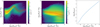 |
Fig. 1. Number of galaxies as a function of their host halo mass and H I mass in the ELUCID SAM catalog. The number in logarithmic scale is represented by different colors. We show the result of central (satellite) galaxies in the left (middle) panel. The mean value and standard deviation are shown together with the color map to illustrate the trend more clearly. The average number of satellite galaxies in each halo as a function of mass is shown in the right panel. |
Together with the number of galaxies represented by different color, we also show the mean value and the standard deviation in Fig. 1. The mean H I mass of the central galaxies clearly peaks around host halo mass Mhalo = 1011.6 M⊙ h−1. Below this, the H I mass is positively correlated to the halo mass, and beyond this peak, the H I mass drops with higher halo mass until Mhalo ∼ 1013 M⊙ h−1. The mean H I mass of satellite galaxies depends weakly on the halo mass. With higher halo mass, the number of satellite galaxies rises up quickly, and the standard deviation of their H I mass also increases. Therefore the total H I mass in a dark matter halo consists of the contribution of the central galaxies and satellite galaxies, which is different for different halo masses.
The H I mass function measured from the ELUCID SAM catalog at z = 0 is shown in Fig. 2. We show the mass function of satellite galaxies and central galaxies separately, as well as the total H I mass function. The Schechter function given in Martin et al. (2010) is shown as a red curve for comparison. The SAM H I mass function fits the Schechter function at MHI > 108 h−1 M⊙ well, but deviates from it at the low-mass end. Overall, the SAM catalog still provides a reasonably similar mass function to that fit from ALFALFA observation.
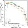 |
Fig. 2. H I mass function measured from the ELUCID SAM catalog at z = 0. The result of central (satellite) galaxy is shown in blue (orange), and the total result is shown in green. The red curve shows the Schechter function provided by Martin et al. (2010), which represents the fitting function of ALFALFA observation. Overall, the H I mass function between the SAM and observation is consistent. |
3.3. HI mass-halo mass relation
To generate the mock 21 cm map, the data product from N-body simulations or fast simulations is usually a dark matter halo catalog. The most popular and simplest information in the halo catalog are the position, the velocity, and the mass of the halo. Therefore it is most useful if we can find an H I mass-halo mass relation that provides the H I mass as a function of halo mass. Figure 3 shows that for low-mass halos, the main contribution to the H I mass comes from the central galaxies, and for high-mass halos, the main contribution comes from satellite galaxies. Although massive halos contain more H I mass in the central galaxies than in every individual satellite galaxies on average, the number of satellite galaxies is so huge that they still contribute most of the H I mass to massive halos. It is very important to consider the satellite galaxy contribution of H I mass in massive halos, which is ignored in HIR4 mock (Asorey et al. 2020). We also compared the H I mass-halo mass relation to the observational results (Guo et al. 2020) at z = 0. The results from the ELUCID galaxy catalog fit to the observation relatively well.
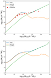 |
Fig. 3. H I mass-halo mass relation at two different redshifts. Upper (lower) panel: H I mass-halo mass relation at z = 0(0.66). The total H I mass is shown as a blue curve, the contribution from central galaxies is shown in orange and the contribution from satellite galaxies is shown in green. Regardless of whether it is at z = 0 or 0.66, the central galaxy always contributes the most H I mass to low-mass halos, and satellite galaxies contribute most of the H I mass in high-mass halos. We also show the observed H I mass-halo mass relation as red dots at z = 0 (Guo et al. 2020) for comparison. |
We first fit the measured H I mass-halo mass relation from the ELUCID SAM catalog using a linear function plus a Gaussian function with free parameters a, b, c, d, and f. Then we derived the parameters as functions of redshift z by assuming that the parameters are linearly related to redshift in 0 < z < 0.66. Then we determined the following analytical formula, which can easily be applied to halo catalogs with the information of the halo mass,
 (1)
(1)
where z is the redshift, mHi is the H I mass in units of M⊙ h−1, and m is the halo mass in units of M⊙ h−1. The halo mass definition is based on a friends-of-friends (FoF) halo finding algorithm, and the linking length is 0.2 times the mean particle separation distance. The fitting result is shown in Fig. 4. The H I mass-halo mass relation is very similar between z = 0 and z = 0.66, therefore the assumption that the parameters are linearly related to redshift in 0 < z < 0.66 is reasonable.
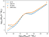 |
Fig. 4. Fit of the measured H I mass-halo mass relation from the ELUCID SAM catalog. The analytical formula is shown as solid lines. The best-fit curve is in the mass range 1010 M⊙ h−1 < Mhalo < 1015 M⊙ h−1. |
4. Tests with ELUCID
4.1. Halo mass threshold
When the mock H I distribution is built, the mass resolution and box size of the halo catalog we use is usually limited. We need to know the effect of a limited mass resolution on the H I power spectrum. This effect can be quantified by the bias of H I gas in the mass-limited sample. The H I gas traces the matter distribution in a biased way. We usually use the bias parameter bHi to describe the difference between H I distribution and the matter distribution. Similarly, the dark matter halos also trace matter distribution in a biased way, and the halo bias is b. It has been addressed in HIR4 (Asorey et al. 2020) that the bias of the H I power spectrum can be calculated as the weighted average of the halo bias,
 (2)
(2)
where b(m, z) represents the halo bias, mHi is the H I mass and m is the halo mass. The halo bias can be calculated by the empirical formula calibrated by N-body simulations (Tinker et al. 2010). The halo bias we used here is scale independent, which means that the resulted H I bias model is also scale independent. In other words, if the H I bias is scale dependent, our bias model cannot provide a proper description.
With the high-resolution ELUCID simulation, we can shed light on whether a scale-independent bias model is a proper description. We selected the galaxies according to their host halo mass with a mass threshold m > 5 × 10⁹ M⊙ h−1, 1 × 10¹⁰ M⊙ h−1, 1 × 10¹¹ M⊙ h−1, 1 × 10¹² M⊙ h−1. In Fig. 5 we show the H I power spectrum of the selected samples and the full sample in the left panel and in the right panel we show the ratio of the H I power spectrum of the selected samples and the full sample. The linear matter power spectrum calculated using Eisenstein & Hu (1998) is shown for reference in cyan color in the left panel. Considering the RSD effect, the positions of the galaxies (x) are mapped to redshift space (s) using the plane-parallel approximation
 (3)
(3)
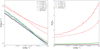 |
Fig. 5. Comparison of power spectrum with different halo mass threshold. On the left, we show the H I power spectrum. On the right, we show the ratio of the power spectrum of the sample with a halo mass threshold and the full sample. The solid curves show the results in real space and the dashed curves show the results in redshift space. Different colors denote different samples with different thresholds. We also include the linear matter power spectrum for reference in cyan color on the left. |
where vlos is the peculiar velocity of the galaxies along line-of-sight. The redshift-space results are shown as dashed lines in Fig. 5. We deducted the shot noise power for the illustration and for the calculation of the power spectrum ratio. Only when the ratio of power spectrum is close to a constant can we safely use the scale-independent halo bias to calculate the H I bias. Considering a scale of 1 degree in the sky, which corresponds to k ∼ 0.5 h Mpc−1 at z ∼ 0.12, the power spectrum ratio of m > 1011 M⊙ h−1 from k ∼ 0 to k ∼ 0.5 h Mpc−1 is close to a constant, but in the m > 1012 M⊙ h−1 case, the ratio cannot be well represented by a constant.
Therefore we conclude that the halo mass resolution to create a mock 21 cm intensity map requires at least ∼1011 M⊙ h−1. The finer the mass resolution, the better.
4.2. Repopulate HI mass
We used the H I mass-halo mass relation introduced in Sect. 3.3 to repopulate the main halos in the ELUCID simulation at z = 0 with H I gas in order to test the performance of our H I HOD model. We generated three types of H I maps and calculated their power spectrum.
-
We used the galaxy (halo) positions in real space, treated the galaxies (halos) as point masses, and calculated the H I distribution in the SAM (HOD) catalog.
-
We used the galaxy (halo) positions in redshift space, treated the galaxies (halos) as point masses, and calculated the H I distribution in the SAM (HOD) catalog.
-
We used the galaxy (halo) positions in redshift space, treated the galaxies (halos) as extended mass due to the H I velocity dispersion inside the galaxies (halos), and calculated the H I distribution in the SAM (HOD) catalog.
We modeled the H I velocity dispersion inside galaxies at z = 0 as
 (4)
(4)
which was also used in Zhang et al. (2020), and is derived from the IllustrisTNG simulation (Villaescusa-Navarro et al. 2018). Usually, we did not consider the H I velocity dispersion inside galaxies (halos) when we created the mock 21 cm intensity map using N-body simulations. Zhang et al. (2020) pointed out that with the proper consideration of this H I velocity dispersion, we can describe the H I mass distribution in redshift space more realistically. Therefore, we made these three types of H I maps for the test. The results are shown in Fig. 6. The power spectrum is shown in the left panel and the ratio of the HOD model and the SAM catalog is shown in the right panel. In the left panel, the dashed lines represent the H I power spectrum measured from the HOD model and the solid lines show the results of the original SAM catalog. The HOD model can recover the H I power spectrum in the SAM catalog overall within a 10% (20%) accuracy up to k = 0.5 h Mpc−1 (k = 0.8 h Mpc−1). Therefore we have validated the method of the HOD model to populate dark matter halos with H I mass.
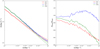 |
Fig. 6. Comparison of the power spectrum of the HOD model and the SAM catalog. On the left, we show the H I power spectrum. The solid lines represent the power spectrum measured from the SAM galaxy catalog, and the dashed lines represent the power spectrum measured from the HOD model. “Real” means the real-space point-mass power spectrum, “red” means the redshift-space point-mass power spectrum, and “red2” means the redshift-space inside the galaxy H I distribution modeled power spectrum (Zhang et al. 2020). On the right, we show the power spectrum ratio of the results of the HOD model and the SAM galaxy catalog. |
5. Mock building with HR4
5.1. Horizon Run 4 catalog
Horizon Run 4 (HR4 for short) is a cosmological N-body simulation with a cubic box size of 3150 Mpc h−1 and 63003 particles (Kim et al. 2015). The HR4 simulation adopted the WMAP5 ΛCDM cosmology, where Ωm = 0.26, ΩΛ = 0.74, h = 0.72, σ8 = 0.79, and ns = 0.96 (Dunkley et al. 2009). The halos are identified with an FoF algorithm with a linking length equal to 0.2 times the particle mean distance in the HR4 simulation. At least 30 particles are required to identify a halo. This means that the minimum halo mass is 2.7 × 10¹¹ M⊙ h−1.
We used the halo light cone catalog and the mock galaxy light cone catalog to generate our mock 21 cm intensity map. In order to generate a full-sky light cone catalog, we typically use the periodic boundary conditions of the simulations to pile up simulation boxes to obtain a deep light cone. This technique introduces some duplicate structures. However, the HR4 simulation box size is so large that there are no periodic structures in z < 0.6 in the full-sky light cone catalog.
The redshift range of BINGO is 0.127 < z < 0.449. Our mock map therefore contains no duplicate structure. In summary, there are four steps in making the mock map.
-
First, we populated H I gas in the galaxy (halo) catalog and calculated the H I density distribution ρHi.
-
Then we calculated the brightness temperature
 (5)
(5)where ρc is the critical density of the Universe (Villaescusa-Navarro et al. 2018).
-
Then we rescaled the map according to the required ΩHi.
-
Finally we smoothed the brightness temperature map with a Gaussian kernel with a full width at half maximum (FWHM) of 40 arcmin, which is due to the beam of BINGO.
5.2. Abundance matching
Halo abundance matching (HAM) and subhalo abundance matching (SHAM) have been widely used to link dark matter halos to galaxies in observations. Under the assumption that more luminous galaxies (with higher H I mass) are populated inside more massive halos (subhalo), we can populate the halos in the simulations with galaxies. This was adopted to generate the HR4 galaxy catalog (Hong et al. 2016). The HR4 galaxy catalog provides the position, velocity, and an “artificial mass-like quantity”, which is also used to estimate the galaxy luminosity with abundance matching. We used the Schechter form of the H I mass function measured from the ALFALFA catalog (Martin et al. 2010),
 (6)
(6)
where mHi is in units of M⊙. We also calculated the abundance of galaxy “mass” in the redshift range 0.127 < z < 0.449 in the HR4 galaxy light cone catalog. By matching the abundance of the galaxy “mass” and the H I mass function, we obtained a H I mass-galaxy “mass” relation. In this way, we populated H I mass in the galaxy catalog. The measurement of the H I mass function from ALFALFA is made at z = 0, which is not compatible with the light cone catalog. It is just an approximate way of populating H I mass in galaxies. Then we sliced the catalog into redshift bins of 10 MHz each. We calculated the density of H I in each redshift using HEALPix pixelization (Gorski et al. 2005) with Nside = 256. Finally, using Eq. (5), we calculated the brightness temperature distribution. This set of mock map is labelled HAM mock map in the following sections.
In Fig. 7, we show a Mollweide projection of the brightness temperature map in the 990 MHz−1000 MHz bin in units of mK as an example. The map represents the H I distribution in real space.
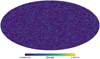 |
Fig. 7. Mollweide projection of the brightness temperature map using the abundance-matching method to populate H I gas in galaxies in real space from 990 MHz to 1000 MHz. |
5.3. HOD population
The abundance-matching method has the following shortcomings: First, Using the H I mass function at z = 0 to match all galaxies at different redshifts is not adequate because the evolution with redshift is ignored and the H I mass is mismatched. Second, The assumption that a galaxy with a higher mass has a higher H I mass may not hold. Third, It is not convenient to calculate the bias from theory to compare with the mock map. Fourth, If only FoF halo catalog (without subhalo catalog) is available, this abundance-matching method does not apply, while many fast simulations only provide FoF halo catalog. Therefore we need to use the HOD approach to obtain the mock map.
With the FoF halo light cone catalog from the HR4 simulation, we can use the H I mass-halo mass relation described by Eq. (1) to populate the H I mass in the halo catalog. We followed the same process as described in the last subsection. We separated the catalog into 30 bins and pixelized the full sky map using HEALPix with Nside = 256. We obtained the brightness temperature map and show it in Fig. 8. This Mollweide projection map extends from 990 MHz to 1000 MHz and represents the real-space distribution of H I gas, in the same way as Fig. 7. Comparing these two maps, we can see that different ways of populating H I gas in galaxies (halos) lead to different results. Although the map looks very similar at a large scale, the brightness temperature fluctuation in the HAM map is much higher than that in the HOD map. This illustrates the different bias of the H I distribution. With the abundance-matching method, H I gas is more clustered than in the HOD method. A more detailed discussion is provided in Sect. 6. With intensity mapping, we can distinguish different ways of H I clustering and occupation in halos.
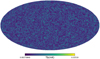 |
Fig. 8. Mollweide projection of the brightness temperature map using the HOD method to populate H I gas in halos in real space from 990 MHz to 1000 MHz. |
5.4. Redshift-space distortion
The intensity map we observe is binned according to frequency, which is determined by the redshift of the 21 cm emission source. Thus, we observe in redshift space rather than real space. We need to consider not only the redshift of emission sources due to the Hubble flow, but also the redshift contribution from the peculiar velocity of the sources. The positions of the 21 cm emission sources are different in redshift space from the positions in real space. This is known as RSD effect, which consists of the Kaiser effect at large scale (Kaiser 1987) and FoG effect at small scale (Jackson 1972). We considered two possible sources of the RSD effect in the mock map.
-
The peculiar velocity of galaxies (halos) as a point source, which mainly contributes to the Kaiser effect,
-
The velocity dispersion inside the halos, which mainly contributes to the FoG effect.
In Fig. 9, we show the Mollweide projection mock map of the brightness temperature adopting the point-source assumption in the upper panel. The result of additionally considering the velocity dispersion is shown in the lower panel. Under the point-source assumption, it is easy to adopt the RSD effect because the redshift of the source can be calculated by
 (7)
(7)
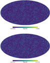 |
Fig. 9. Mollweide projection of the brightness temperature map using the HOD method to populate H I gas in halos in redshift space from 990 MHz to 1000 MHz. We only considered the velocity of halos as a point source in the upper panel, which mainly only contains Kaiser effect. Lower panel: we considered the velocity dispersion of H I gas in the sources, which means that the FoG effect is taken into account. |
where z is the redshift of the point source calculated according to its distance to the observer and Hubble’s law, which is provided in the light cone catalog, vr is the peculiar velocity along the line-of-sight direction, and c is the speed of light. Then we can bin the sources according to their redshift z′, calculate the H I density with Nside = 256 HEALPix pixelization and calculate the corresponding brightness temperature. When this is compared to the real-space mock map after considering the RSD effect, some of the sources are moved away from their real-space frequency range, and some of them are moved into the frequency bin. Thus, this shows slightly different large-scale structures in the real space mock map and in the redshift-space mock map.
The mock map considering the velocity dispersion of H I gas in halos is built following the steps described below.
-
We calculated the velocity dispersion of H I gas in each halo according to the halo mass m and real redshift z,
 (8)
(8)which was fitted from IllustrisTNG simulation (Villaescusa-Navarro et al. 2018) and adopted in Zhang et al. (2020) (this fitting formula uses multiple data points at different redshifts, and the calculated result at z = 0 is not exactly the same as Eq. (4)).
-
We calculated the corresponding comoving distance variance
 .
. -
For a given redshift bin from z1 to z2, where z1 < z2, we calculated the corresponding comoving distance range from s1 to s2, and selected the halos within the range s1 − 3δs and s2 + 3δs in redshift space,
-
We calculated the H I mass contribution w from the selected halos in this given bin for a given halo at sh,
 (9)
(9) -
We calculated the H I density in this bin and the related brightness temperature.
In this way, we assumed that the mass distribution of H I in one halo in redshift space follows a Gaussian distribution. This process can provide a rough estimate of FoG effect in the mock map.
5.5. Rescale the map
The average brightness temperature  can be calculated from the mock maps at different redshifts. It also represents the H I abundance ΩHi because the mean temperature is proportional to it. The relation of
  and ΩHi is
 (10)
(10)
Because we neglected the contribution from halos whose mass is lower than the resolution in the mock map, we may have missed some of the H I gas in small halos. On the other hand, we may also have overestimated the H I mass in halos in the comparison to the real observation for various reasons, for instance, we may have overestimated the H I mass-halo mass relation. Therefore we need to rescale the maps to meet the requirement of ΩHi. We can rescale the maps according to the required ΩHi value by applying 
6. Results of the mock
6.1. Angular power spectra
We address the effect of different ways of linking H I gas with galaxies (halos) and the effect of RSD an angular power spectrum in this subsection. We also determine whether we can identify this difference with the BINGO telescope.
In Fig. 10, we showed the zoom-in view of a 10 × 10 deg2 brightness temperature map of the full-sky mock map from 990 MHz to 1000 MHz. We compared the map generated using the HOD method (labeled HOD) and the abundance-matching method (labeled HAM) and rescaled the HAM map to the same ΩHi as the HOD map (labeled Re-HAM). We also showed the map smoothed with a Gaussian kernel with an FWHM = 40 arcmin. The same color map is shown in each row for comparison. The Tb contrast in the HAM map is clearly much higher than that in the HOD map, which can be more easily identified in the Re-HAM map. In the HAM map, more H I gas is located inside clusters than in the HOD map. Because the bias of high-mass halos is higher than that of low-mass halos, we expect that with the same ΩHi, the angular power spectrum of the mock map generated with the abundance-matching method is higher than the map generated using HOD.
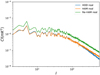 |
Fig. 10. Zoom-in view of the central 10 × 10 deg2 brightness temperature distribution of the mock map from 990 MHz to 1000 MHz. |
Figure 11 verifies our expectation. Re-HAM and HOD share the same ΩHi, but the angular power spectrum of the Re-HAM mock map is much higher than that of the HOD mock map. The HAM mock shows a very similar angular power spectrum to the HOD mock by coincidence. Moreover, at large l (l > 200), the real-space angular power spectrum of the HAM mock is slighter larger than the HOD mock. This phenomenon is also shown in Fig. 6. We know that in the HOD mock, the H I gas is assumed to be located at the center of the halo, without any substructures. In the mocks that contain subhalos, however, the subhalo distribution inside the main halos leads to additional clustering at small scales, which is known as the one-halo term. This can be seen when the HR4 HAM mock and HR4 HOD mock in Fig. 11 are compared. It can also be seen when ELUCID SAM mock and ELUCID HOD mock in Fig. 6 are compared. Therefore it is expected that at small scales, the real-space power spectrum of HOD mock has a smaller amplitude as the HAM mock or SAM mock in real space. However, when RSD effect is considered, because the subhalos in halos also move randomly in the frame of the center of mass of the main halo, the FoG effect suppresses the power spectrum at small scales. Thus, in the red mock, the higher power from the one-halo term and the lower power from the FoG counter each other, and the power spectrum of the HOD mock and SAM from the ELUCID simulation approach each other. Furthermore, in the red2 mock, the FoG effect is taken into account in the HOD mock, and the difference between HOD and SAM is again revealed.
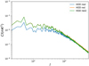 |
Fig. 11. Comparison of the angular power spectrum of the HOD mock, HAM mock, and Re-HAM mock in real space. With the same ΩHi, the Re-HAM mock has a higher angular power spectrum than the HOD mock, which means that it has a higher bias. Although very close at large scales, HAM mock has higher angular power spectrum than the HOD mock at small scales because of the substructures in the HAM mock. |
In Fig. 12, we show the comparison of the HOD real-space mock (labeled “real”), the HOD redshift-space point-source mock (labeled “red”), and HOD redshift-space mock that includes the FoG effect (labeled “red2”). The angular power spectrum difference between the real and the red mock is clear at large scales because of the Kaiser effect, but the difference between the red mock and the red2 mock due to FoG effect at small scales is not significant. This is because of the bin width of the mock is 10 MHz, that corresponds to more than 20 Mpc h−1, while the typical velocity dispersion is not higher than 1000 km s−1, which roughly corresponds to 10 Mpc h−1 in redshift space. Therefore the power spectrum suppression introduced by the velocity dispersion is averaged out by the large bin width.
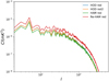 |
Fig. 12. Comparison of the angular power spectrum of the HOD mock in real space and redshift space. The power in redshift space is higher than in real space at large scales because of the Kaiser effect. Regardless of whether we treat the H I gas in halos as point sources (red) or extended sources due to internal velocity dispersion (red2) in redshift space, the difference between them is not significant. |
In Fig. 13, we compare the angular power spectrum of the mocks smoothed by a Gaussian kernel with an FWHM = 40 arcmin, which is the beam size of BINGO. After smoothing, the difference at small scales is easily covered. The difference of the bias can still be clearly identified by comparing HOD mock and Re-HAM mock, which share the same ΩHi value. Therefore we can answer the questions raised at the beginning of this subsection.
-
Different ways of linking H I gas with galaxies (halos) lead to a different bias and one-halo term. The bias difference can be seen in the total power of angular power spectrum and the difference of one-halo term can be seen at small scales.
-
The Kaiser effect leads to a higher angular power spectrum at large scales. The FoG effect leads to a suppression of the power spectrum at small scales, but cannot be distinguished due to 10 MHz bin size.
-
Gaussian kernel smoothing eliminates the difference at small scales, but the bias difference shown at all scales and the Kaiser effect shown at large scales can still be easily identified.
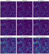 |
Fig. 13. Angular power spectrum of the HOD mock, HAM mock, and Re-HAM mock in redshift space. Re-HAM mock is clearly higher due to a higher bias. The difference between the HAM mock and HOD mock due to the one-halo term and the difference between red mock and red2 mock due to the FoG effect at small scales is not significant because of smoothing introduced by the Gaussian kernel with an FWHM = 40 arcmin. |
6.2. Pixel histogram
We have shown that the brightness temperature fluctuation in the HAM mock is higher than in the HOD mock in Fig. 10. More quantitatively, we calculated the histogram of the pixels in the unsmoothed mock map. In the upper panel of Fig. 14, we show the histogram of the pixels. We excluded all the pixels that are zero. As expected, there are more extremely high brightness temperature pixels in the HAM mock than in the HOD mock.
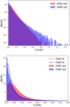 |
Fig. 14. Pixel histogram of the brightness temperature distribution of the mock map from 990 MHz to 1000 MHz in redshift space. Upper panel: histogram comparison of the HOD map and the HAM map from 0 mK to 1.5 mK. Lower panel: we zoom in to the range from 0 mK to 0.4 mK. The lognormal fitted curves are also shown. The HAM map clearly has more extremely high brightness temperature pixels, as expected from Fig. 10. |
On the other hand, the lognormal distribution was widely used to simulate dark matter tracer fields (Xavier et al. 2016), which is the 21 cm intensity map in our case. We calculated the histogram of the pixels from 0 mK to 0.4 mK and fit them with the lognormal distribution using the stats routine in scipy (Virtanen et al. 2020). The result is shown in the lower panel of Fig. 14. We found that the lognormal distribution can represent the measured results from our mock map reasonably well. This means that using a lognormal distribution to simulate the brightness temperature map is reasonable, but has clear limitations as well.
The difference between the pixel histogram of the HOD mock and the HAM mock shows that the way in which the H I gas is distributed inside the halos can largely affect the intensity map, not only in the angular power spectrum, but also in other statistical measurements.
6.3. Lognormal fitting
The lognormal distribution can provide a reasonable fitting to the pixel histogram of the mock map, both in redshift space and in real space. Furthermore, after we considered the 40 arcmin Gaussian kernel smoothing for the mock map, we found that the lognormal function can fit the pixel histogram very well. We illustrate one slice as an example in Fig. 15. We fit the histogram by a lognormal distribution using the stats routine in scipy (Virtanen et al. 2020). For every redshift bin, we fit the histogram with the lognormal distribution and show the parameters in Fig. 15. The lognormal probability density function is
 (11)
(11)
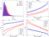 |
Fig. 15. Pixel histogram of the brightness temperature distribution and related lognormal fitting results. Upper left panel: histogram of the pixels of the brightness temperature distribution of the redshift-space mock map from 990 MHz to 1000 MHz smoothed by a 40 arcmin Gaussian kernel. After smoothing, the histogram can be very well fit by the lognormal distribution. The fitted parameters, s, loc, and scale, are shown as a function of the redshift (frequency) in the other three panels. For each of them we also fit a parabola function, which is a good fit. The lognormal fitted parameters are shown in red for the HOD mock and in blue for the HAM mock. Crosses represent the real-space mock and dots the redshift-space mock. The parabola fitting curves are shown in red for the HOD mock and in blue for the HAM mock. Solid lines show the real-space mock, and dashed lines show the redshift-space mock. |
where the x variable is given by Tb in our case.
We used the parabola function, f(z)=a + bz + cz2 to fit these three parameters of the lognormal distribution as a function of redshift z. The fit results are given in Table 1.
Parabola fitting parameters of lognormal parameters as a function of redshift z.
Based on these parameters, a similar mock map can be generated using the lognormal distribution (Xavier et al. 2016). This is helpful for further study and comparison.
6.4. Effect of the bin size
As discussed in Sect. 6.1, different ways of populating H I gas in galaxies (halos) will lead to different biases and one-halo term, and the bin width of 10 MHz will largely wipe out the FoG effect. One step further, it is interesting to ask whether if we used a different bin width, for example, 2 MHz or 5 MHz, the conclusion would be. A more significant FoG effect might be visible, or a different small scale power introduced by the one-halo term with a smaller bin width. To answer this question, we generated the mock map with the HOD and HAM method in a 2 MHz bin width and 5 MHz bin width, following the same steps as we used to generate the 10 MHz bin width mock map.
In Fig. 16 we show the comparison of the angular power spectrum of the mocks with 10 MHz, 5 MHz, and 2 MHz. For better comparison, we took the frequency range from 990 MHz to 1000 MHz, which consists of one bin in the 10 MHz mock, two bins in the 5 MHz mock, and five bins in the 2 MHz mock. We took the average of the angular power spectrum measured from this one (two and five) bin(s) of 10 (5 and 2) MHz mocks. We also amplified the results to keep the curves of different bin width separated for better illustration. The higher angular power spectrum of the HAM mocks compared to the HOD mocks at small scales (l > 100) is evident. The angular power spectrum of the HOD mocks compared to HAM mocks is lower by more than 10% at l > 300. It is also obvious that the difference hardly depends on the bin width. This is expected because regardless of whether the difference of the small-scale power is due to scale-dependent bias or the one-halo term, it is isotropic. The width of the frequency bin is expected to play only a little role in the power spectrum.
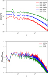 |
Fig. 16. Comparison of HOD and HAM mocks in real space shown with 10 (5 and 2) MHz in red (blue and green). Upper panel: HOD results are shown as thick solid lines, and the HAM results are shown as faint solid lines. For better illustration, we artificially amplified the curves by 0.5 (1 and 2) times for 10 (5 and 2) MHz results. Lower panel: ratio of the angular power spectrum of the HOD mocks and HAM mocks. Clearly, HAM mocks have a higher angular power spectrum at small scales, and it depends weakly on the bin width. |
In contrast, the FoG effect is anisotropic. The FoG effect points toward the line-of-sight direction. We expect to see a stronger suppression due to the FoG effect at small scales with a smaller bin width because there is less smoothing. The result is shown in Fig. 17, which is exactly what we have expected. We assumed a point source in the red mock and took the velocity dispersion into account in the red2 mock. Therefore the FoG effect is modeled in the red2 mock. The FoG effect is very clear in the 2 MHz mock, it is weaker in the 5 MHz mock, and it is almost indistinguishable in the 10 MHz mock. We conclude that a smaller frequency bin width is very effective in identifying the FoG effect in 21 cm intensity-mapping observations. However, we also note that with a smaller bin width, the noise level is also higher. Therefore it is an open question whether we can identify the FoG effect in the real observations with BINGO.
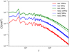 |
Fig. 17. Comparison of the red (point-source assumption) HOD mock and the red2 (velocity dispersion induced FoG effect modeled) HOD mock shown with 10 (5 and 2) MHz in red (blue and green). The red results are shown as thick solid lines, and the red2 results are shown as faint solid lines. For better illustration, we artificially amplified the curves by 0.5 (1 and 2) times for 10 (5 and 2) MHz results. The FoG suppression at small scales is clearer with a smaller bin width. |
6.5. Comparison with UCLCl
When we take the mock maps and the measured angular power spectrum as a real observation, we need a fast model prediction to compare this with the map and see whether we can fit it to the observation. This is essential for parameter fitting and cosmological parameter constraints. UCLCl (Unified Cosmological Library for Cℓs) is a package that calculates the angular power spectra (McLeod et al. 2017; Loureiro et al. 2019) from the power spectrum of density fluctuations through
 (12)
(12)
where Wl(k) is the window function that absorbs all the processes involved in the evolution, convolution, and the projection effects, and Δ2(k) is the dimensionless matter power spectrum. By using the linear perturbation calculation of the matter power spectrum, we obtain the linear angular power spectrum. By using the halofit nonlinear correction (Takahashi et al. 2012), we can take the one-halo term nonlinear effect into account. We calculated the angular power spectrum using the UCLCl package with the cosmological parameters consistent with the HOD mock.
In Fig. 18, we compare the results of the UCLCl and our HOD mock measurements in redshift space. The point-source assumption was taken in this HOD mock for comparison. The HOD mock results are higher than the linearly calculated results, but they are lower than the halofit corrected results at small scales. At large scales, the UCLCl results are consistent with the HOD mock except for the obvious fluctuations due to cosmic variance. At lower redshift (higher frequency), we can see a larger small-scale nonlinear correction than at higher redshift (lower frequency). There are two reasons for this. One reason is that at higher redshift, the one-halo term plays a smaller role than at lower redshift. The other reason is that at lower redshift, the shell of the H I distribution that we can measure is closer to us, which means that at lower redshifts we can see more details from small scales with the same angular resolution when compared to higher redshift shells.
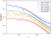 |
Fig. 18. Angular power spectrum of the HOD mocks (solid faint curves) compared to the calculation with the UCLCl code with a linear calculation (dashed lines) and halofit nonlinear correction (dotted lines) in redshift space. Red (orange, green, and blue) lines show the result from 960 (1050, 1150, and 1160) MHz to 970 (1060, 1160, and 1260) MHz, averaged at 965 (1055, 1155, and 1255) MHz, which are amplified by 0.25 (0.5, 1, and 2) times for better illustration. HOD mock measurements are higher than the linear calculation, but lower than the halofit calculation at small scales. |
If we take the HOD mock as a benchmark, the linear case has underestimated the angular power spectrum at small scales and the halofit correction has overestimated the angular power spectrum. At higher redshift, the UCLCl calculation is closer to the measurements of the HOD mock. At l < 80, the UCLCl linearly calculated results, which adopted the linear bias assumption, can fit the HOD mock from 1250 MHz to 1260 MHz. From 960 MHz to 970 MHz, the UCLCl linear calculation can fit the HOD mock result up to l < 200. This comparison clearly tells us the shortcoming of our modeling for the 21 cm intensity-mapping angular power spectrum using the UCLCl package. Without further improvement in the modeling at small scales and a better understanding of the H I distribution in halos, it is hard to use the full information of the angular power spectrum at l > 80 at the lowest redshift and l > 200 at the highest redshift for BINGO.
6.6. HI bias and abundance
The overall amplitude of the angular power spectra of 21 cm intensity mapping is closely related to ΩHi and bHi. Therefore, observations constrain these parameters. The detailed forecast is provided in our companion Paper VII (Costa et al. 2022). Here we provide the answer of the mock map for the future parameter fitting and pipeline building. We calculated the ΩHi in each mock map by adding all the H I mass in each redshift bin, and then divided it by the volume of each bin. We show ΩHi as a function of frequency (redshift) in Fig. 19. The measurement of the HOD mock is shown as dotted lines, and the HAM mock is shown as dashed lines. The population of the H I mass is different in the real-space mock map and the in the redshift-space mock map in the same frequency bin because of RSD effect. We illustrate the result of real-space mock and redshift-space mock in different colors, but there is clearly little difference between real space and redshift space. The RSD has little effect on the ΩHi in each bin. We provided a parabola fitting to the real-space mocks, which gives
 (13)
(13)
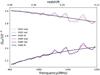 |
Fig. 19. ΩHi as a function of frequency (redshift) in our mock map. The dotted lines show the result of the HOD mock, and the dashed curves show the result of the HAM mock. “Real” means the real-space mock, and “red” means the redshift-space mock under the point-source assumption. The solid black lines show the parabola fitting results to the real-space mock. |
for the HOD mock and
 (14)
(14)
for the HAM mock, shown as solid black lines.
For the HOD mock, we used the publicly available python package COLOSSUS (Diemer 2018) to calculate the bias of each halo using the empirical relation provided by Tinker et al. (2010), and by considering the following relation in real space:
 (15)
(15)
we estimated the bias of the HAM mock. We show the bias bHi as a function of frequency (redshift) in Fig. 20. The crosses represent the result of the HOD mock and the dots represent the result of the HAM mock. Because the real-space and redshift-space results are almost identical, we just show the results of the real-space mock for better illustration. Similarly, we also provide the parabola fitting results
 (16)
(16)
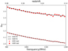 |
Fig. 20. bHi as a function of frequency (redshift) in our mock map. The crosses show the result of the HOD mock and the dots show the result of the HAM mock. The real-space and redshift-space mock bias are measured, and they are almost identical. The solid black lines show the parabola fitting results. |
for the HOD mock and
 (17)
(17)
for the HAM mock, shown as solid black lines. The large difference in the bias of the HOD mock and the HAM mock shows that different ways of H I gas occupation can lead to a very different linear bias, which is observable in the angular power spectrum. The 21 cm intensity mapping can also tell us about the H I gas distribution, which is related to the galaxy formation and evolution.
The fitting formula has three advantages.
-
It is useful when the map is to be reproduced with other methods, such as a Gaussian realization or FLASK, which can easily generate a large number of realizations to construct a covariance matrix.
-
It can largely reduce the number of free parameters for ΩHi and bHi with the fitting formula, when maps at many different redshifts are used.
-
This fitting formula is independent of the number of bins. It is useful when we need to change the number of bins.
7. Summary and discussion
We have introduced the method of building mock 21 cm intensity maps using N-body simulation data. In summary, we have achieved the following points:
-
We used the ELUCID N-body simulation and its semianalytical galaxy catalog to study the H I halo occupation distribution. We concluded that for halos less massive than 1012 M⊙ h−1, the main contribution of H I gas comes from the central galaxies. For halos more massive than 1013 M⊙ h−1, the main contribution of H I gas comes from the satellite galaxies. Neglecting the H I contribution in satellite galaxies is not a good approximation.
-
We provided a good fitting formula of the H I mass-halo mass relation. This facilitates populating H I gas in dark matter halos. The fitting function is given by Eq. (1).
-
The HOD method was verified using the ELUCID simulation by comparing it to the SAM galaxy catalog. With a 10% accuracy, the power spectrum of the HOD-repopulated H I distribution is correct up to k = 0.4 h Mpc−1.
-
The mass resolution of the N-body simulation can lead to scale-dependent bias. With the halo mass limit down to about 1011 M⊙ h−1, the linear bias assumption, which assumes a constant bias number, is still valid. The linear bias assumption is not valid with the 1012 M⊙ h−1 halo mass limit. This sets a resolution requirement for the N-body simulation to be used to build the H I mock map.
-
Using HR4 simulation, we built the full-sky 21 cm intensity mock maps that extend from 960 MHz to 1260 MHz, and cover the range of BINGO (from 980 MHz to 1260 MHz). Both the HOD method and abundance-matching (HAM) method were applied to obtain two types of mocks.
-
The RSD was taken into consideration, we introduced a method that considers the point-source RSD and a method that considers the velocity dispersion to account for the FoG effect.
-
The lognormal distribution can provide a reasonable fitting to the pixel histogram of the mock map. If the map is smoothed by a 40 arcmin Gaussian kernel, the fitting will be very good.
-
We provided the lognormal fitting parameters for our mock maps. A further parabola fitting to the lognormal parameters as functions of redshift was made. The fitting results are given. It is easy to realize a similar brightness temperature distribution with the distribution using our parameters.
-
We discussed the effect of Gaussian beam smoothing, RSD, and the difference of the HOD mock and HAM mock by comparing the angular power spectrum. Different bias and Kaiser effect can be distinguished. The nonlinear effect at small scales and the FoG effect are not important if the 40 arcmin Gaussian smoothing is taken into account.
-
The effect of different frequency bin sizes was discussed. The FoG effect can be more easily identified with a smaller bin size. A different bin size has little effect on distinguishing between HOD mock and HAM mock.
-
The theoretical calculation was made using the UCLCl package and was compared to our mock map measurements. We found that the UCLCl results can fit the mock at large scales, but it failed at small scales. The lower the redshift, the worse. They fit well at l < 80 for the highest frequency bin and at l < 200 for the lowest frequency bin of BINGO. The linear theory calculation has underestimated the angular power spectra at small scales and the halofit nonlinear correction has overestimated it. We need a better modeling to make full use of the whole range of the angular power spectra.
-
We provided the measurement of ΩHi and bHi as a function of frequency (redshift) in the HOD mock and HAM mock. The parabola function can provide very good fit to the measurements. The fit functions for each case are listed in Sect. 6.6.
In addition to constraining cosmological parameters, 21 cm intensity mapping is expected to constrain the astrophysical processes related to H I gas. There is no conclusion about the best method. HAM and HOD, these two different methods we to populate H I gas in halos, can be regarded as valid tests. Because we can distinguish HAM from HOD using 21 cm intensity mapping by constraining the bias parameter, it proves the ability of distinguishing the H I population in halos. The mock we generated here will serve as the source signal to test the BINGO data analysis pipeline. This will include parameter fitting, BAO signal fitting and many other methods developed for intensity mapping.
The method we introduced here will be useful in building mocks based on fast simulations such as COLA-HALO (Koda et al. 2016). After generating hundreds of mocks, we can measure the covariance matrix, which is essential to estimate the cosmological parameters. On the other hand, this methodo can also be applied for other 21 cm intensity-mapping experiments such as the SKA. As a next step, we will combine the foreground, noise and mask of BINGO to generate a more realistic mock map to test our data analysis pipeline. In the future, we will also include more effects that might change the map, such as radio point sources, lensing effects, and gravitational redshift. By continuously making more realistic mock maps, we can improve the understanding of intensity mapping and provide a better data challenge for the pipeline.
Acknowledgments
This work was supported by the Ministry of Science and Technology of China (grant nos. 2018YFA0404601) and National Natural Science Foundation of China (grant nos. 11973033, 11835009). The BINGO project is supported by FAPESP grant 2014/07885-0; the support from CNPq is also gratefully acknowledged (E.A.). C.A.W. acknowledges a CNPq grant 2014/313.597. T.V. acknowledges CNPq Grant 308876/2014-8. J.Z. was supported by IBS under the project code, IBS-R018-D1. C.P.N. would like to thank São Paulo Research Foundation (FAPESP), grant 2019/06040-0, for financial support. A.A.C. acknowledges financial support from the China Postdoctoral Science Foundation, grant number 2020M671611. F.B.A. acknowledges the UKRI-FAPESP grant 2019/05687-0, and FAPESP and USP for Visiting Professor Fellowships where this work has been developed. R.G.L. thanks CAPES (process 88881.162206/2017-01) and the Alexander von Humboldt Foundation for the financial support. A.R.Q., F.A.B., L.B., and M.V.S. acknowledge PRONEX/CNPq/FAPESQ-PB (Grant no. 165/2018). H.X. and Z.Z. are supported by the Ministry of Science and Technology of China (grant nos. 2018YFA0404601 and 2020SKA0110200), and the National Science Foundation of China (grant nos. 11621303, 11835009 and 11973033). K.S.F.F. thanks São Paulo Research Foundation (FAPESP) for financial support through grant 2017/21570-0. V.L. acknowledges the postdoctoral FAPESP grant 2018/02026-0. L.S. is supported by the National Key R&D Program of China (2020YFC2201600). The Kavli IPMU is supported by World Premier International Research Center Initiative (WPI), MEXT, Japan.
References
- Abdalla, E., Ferreira, E. G. M., Landim, R. G., et al. 2022a, A&A, 664, A14 (Paper I) [NASA ADS] [CrossRef] [EDP Sciences] [Google Scholar]
- Abdalla, F. B., Marins, A., Motta, P., et al. 2022b, A&A, 664, A16 (Paper III) [NASA ADS] [CrossRef] [EDP Sciences] [Google Scholar]
- Alonso, D., Ferreira, P. G., & Santos, M. G. 2014, MNRAS, 444, 3183 [NASA ADS] [CrossRef] [Google Scholar]
- An, R., Costa, A. A., Xiao, L., Zhang, J., & Wang, B. 2019, MNRAS, 489, 297 [NASA ADS] [CrossRef] [Google Scholar]
- Anagnostopoulos, F. K., Basilakos, S., & Saridakis, E. N. 2019, Phys. Rev. D, 100, 083517 [NASA ADS] [CrossRef] [Google Scholar]
- Asorey, J., Parkinson, D., Shi, F., et al. 2020, MNRAS, 495, 1788 [NASA ADS] [CrossRef] [Google Scholar]
- Becker, R. H., Fan, X., White, R. L., et al. 2001, AJ, 122, 2850 [NASA ADS] [CrossRef] [Google Scholar]
- Bigot-Sazy, M. A., Ma, Y. Z., Battye, R. A., et al. 2016, in HI Intensity Mapping with FAST, eds. L. Qain, & D. Li, ASP Conf. Ser., 502, 41 [NASA ADS] [Google Scholar]
- Chen, X. 2012, Int. J. Mod. Phys. Conf. Ser., 12, 256 [NASA ADS] [CrossRef] [Google Scholar]
- Cheng, G., Ma, Y., Wu, F., Zhang, J., & Chen, X. 2020, Phys. Rev. D, 102, 043517 [NASA ADS] [CrossRef] [Google Scholar]
- Costa, A. A., Xu, X.-D., Wang, B., & Abdalla, E. 2017, JCAP, 2017, 028 [CrossRef] [Google Scholar]
- Costa, A. A., Landim, R. G., Novaes, C. P., et al. 2022, A&A, 664, A20 (Paper VII) [NASA ADS] [CrossRef] [EDP Sciences] [Google Scholar]
- Cunnington, S., Pourtsidou, A., Soares, P. S., Blake, C., & Bacon, D. 2020, MNRAS, 496, 415 [NASA ADS] [CrossRef] [Google Scholar]
- Diemer, B. 2018, ApJS, 239, 35 [NASA ADS] [CrossRef] [Google Scholar]
- Dunkley, J., Komatsu, E., Nolta, M. R., et al. 2009, ApJS, 180, 306 [NASA ADS] [CrossRef] [Google Scholar]
- Eisenstein, D. J., & Hu, W. 1998, ApJ, 496, 605 [Google Scholar]
- Fan, X., Strauss, M. A., Becker, R. H., et al. 2006a, AJ, 132, 117 [NASA ADS] [CrossRef] [Google Scholar]
- Fan, X., Carilli, C. L., & Keating, B. 2006b, ARA&A, 44, 415 [Google Scholar]
- Fornazier, K. S. F., Abdalla, F. B., Remazeilles, M., et al. 2022, A&A, 664, A18 (Paper V) [NASA ADS] [CrossRef] [EDP Sciences] [Google Scholar]
- Gorski, K. M., Hivon, E., Banday, A. J., et al. 2005, ApJ, 622, 759 [Google Scholar]
- Guo, H., Li, C., Zheng, Z., et al. 2017, ApJ, 846, 61 [NASA ADS] [CrossRef] [Google Scholar]
- Guo, H., Jones, M. G., Haynes, M. P., & Fu, J. 2020, ApJ, 894, 92 [NASA ADS] [CrossRef] [Google Scholar]
- Hall, A., Bonvin, C., & Challinor, A. 2013, Phys. Rev. D, 87, 064026 [NASA ADS] [CrossRef] [Google Scholar]
- Hong, S. E., Park, C., & Kim, J. 2016, ApJ, 823, 103 [NASA ADS] [CrossRef] [Google Scholar]
- Hu, W., Wang, X., Wu, F., et al. 2020, MNRAS, 493, 5854 [NASA ADS] [CrossRef] [Google Scholar]
- Icaza-Lizaola, M., Vargas-Magaña, M., Fromenteau, S., et al. 2020, MNRAS, 492, 4189 [NASA ADS] [CrossRef] [Google Scholar]
- Jackson, J. C. 1972, MNRAS, 156, 1P [CrossRef] [Google Scholar]
- Jullo, E., de la Torre, S., Cousinou, M. C., et al. 2019, A&A, 627, A137 [NASA ADS] [CrossRef] [EDP Sciences] [Google Scholar]
- Kaiser, N. 1987, MNRAS, 227, 1 [Google Scholar]
- Kim, J., Park, C., L’Huillier, B., & Hong, S. E. 2015, J. Korean Astron. Soc., 48, 213 [Google Scholar]
- Klypin, A., Yepes, G., Gottlöber, S., Prada, F., & Heß, S. 2016, MNRAS, 457, 4340 [Google Scholar]
- Koda, J., Blake, C., Beutler, F., Kazin, E., & Marin, F. 2016, MNRAS, 459, 2118 [NASA ADS] [CrossRef] [Google Scholar]
- Kovetz, E. D., Viero, M. P., Lidz, A., et al. 2017, ArXiv e-prints [arXiv:1709.09066] [Google Scholar]
- Liccardo, V., de Mericia, E. J., Wuensche, C. A., et al. 2022, A&A, 664, A17 (Paper IV) [NASA ADS] [CrossRef] [EDP Sciences] [Google Scholar]
- Loureiro, A., Moraes, B., Abdalla, F. B., et al. 2019, MNRAS, 485, 326 [NASA ADS] [CrossRef] [Google Scholar]
- Luo, Y., Kang, X., Kauffmann, G., & Fu, J. 2016, MNRAS, 458, 366 [NASA ADS] [CrossRef] [Google Scholar]
- Martin, A. M., Papastergis, E., Giovanelli, R., et al. 2010, ApJ, 723, 1359 [NASA ADS] [CrossRef] [Google Scholar]
- McLeod, M., Balan, S. T., & Abdalla, F. B. 2017, MNRAS, 466, 3558 [NASA ADS] [CrossRef] [Google Scholar]
- Naiman, J. P., Pillepich, A., Springel, V., et al. 2018, MNRAS, 477, 1206 [Google Scholar]
- Nelson, D., Pillepich, A., Springel, V., et al. 2018, MNRAS, 475, 624 [Google Scholar]
- Nelson, D., Springel, V., Pillepich, A., et al. 2019, Comput. Astrophys. Cosmol., 6, 2 [Google Scholar]
- Padmanabhan, H., & Refregier, A. 2017, MNRAS, 464, 4008 [NASA ADS] [CrossRef] [Google Scholar]
- Paul, N., Choudhury, T. R., & Paranjape, A. 2018, MNRAS, 479, 1627 [NASA ADS] [CrossRef] [Google Scholar]
- Pillepich, A., Nelson, D., Hernquist, L., et al. 2018, MNRAS, 475, 648 [Google Scholar]
- Pritchard, J. R., & Loeb, A. 2012, Rep. Progr. Phys., 75, 086901 [CrossRef] [Google Scholar]
- Prochaska, J. X., Herbert-Fort, S., & Wolfe, A. M. 2005, ApJ, 635, 123 [NASA ADS] [CrossRef] [Google Scholar]
- Santos, M., Bull, P., Alonso, D., et al. 2015, Advancing Astrophysics with the Square Kilometre Array (AASKA14), 19 [Google Scholar]
- Sarkar, D., & Bharadwaj, S. 2019, MNRAS, 487, 5666 [NASA ADS] [CrossRef] [Google Scholar]
- Seehars, S., Paranjape, A., Witzemann, A., et al. 2016, JCAP, 2016, 001 [CrossRef] [Google Scholar]
- Smoot, G. F., & Debono, I. 2017, A&A, 597, A136 [NASA ADS] [CrossRef] [EDP Sciences] [Google Scholar]
- Springel, V., Pakmor, R., Pillepich, A., et al. 2018, MNRAS, 475, 676 [Google Scholar]
- Takahashi, R., Sato, M., Nishimichi, T., Taruya, A., & Oguri, M. 2012, ApJ, 761, 152 [Google Scholar]
- Tinker, J. L., Robertson, B. E., Kravtsov, A. V., et al. 2010, ApJ, 724, 878 [NASA ADS] [CrossRef] [Google Scholar]
- Vanderlinde, K., & Chime Collaboration 2014, BAAS, 46, 101.02 [Google Scholar]
- Villaescusa-Navarro, F., Genel, S., Castorina, E., et al. 2018, ApJ, 866, 135 [NASA ADS] [CrossRef] [Google Scholar]
- Virtanen, P., Gommers, R., Oliphant, T. E., et al. 2020, Nat. Meth., 17, 261 [Google Scholar]
- Wang, H., Mo, H. J., Yang, X., et al. 2016, ApJ, 831, 164 [Google Scholar]
- Wolfe, A. M., Gawiser, E., & Prochaska, J. X. 2005, ARA&A, 43, 861 [NASA ADS] [CrossRef] [Google Scholar]
- Wuensche, C. A., & the BINGO Collaboration 2019, J. Phys. Conf. Ser., 1269, 012002 [NASA ADS] [CrossRef] [Google Scholar]
- Wuensche, C. A., Villela, T., Abdalla, E., et al. 2022, A&A, 664, A15 (Paper II) [NASA ADS] [CrossRef] [EDP Sciences] [Google Scholar]
- Wyithe, J. S. B., Loeb, A., & Geil, P. M. 2008, MNRAS, 383, 1195 [Google Scholar]
- Xavier, H. S., Abdalla, F. B., & Joachimi, B. 2016, MNRAS, 459, 3693 [NASA ADS] [CrossRef] [Google Scholar]
- Yang, W., Shahalam, M., Pal, B., Pan, S., & Wang, A. 2019, Phys. Rev. D, 100, 023522 [NASA ADS] [CrossRef] [Google Scholar]
- Zafar, T., Péroux, C., Popping, A., et al. 2013, A&A, 556, A141 [NASA ADS] [CrossRef] [EDP Sciences] [Google Scholar]
- Zhang, J., Costa, A. A., Wang, B., et al. 2020, ApJ, 895, 34 [NASA ADS] [CrossRef] [Google Scholar]
All Tables
Parabola fitting parameters of lognormal parameters as a function of redshift z.
All Figures
|
Fig. 1. Number of galaxies as a function of their host halo mass and H I mass in the ELUCID SAM catalog. The number in logarithmic scale is represented by different colors. We show the result of central (satellite) galaxies in the left (middle) panel. The mean value and standard deviation are shown together with the color map to illustrate the trend more clearly. The average number of satellite galaxies in each halo as a function of mass is shown in the right panel. |
| In the text | |
|
Fig. 2. H I mass function measured from the ELUCID SAM catalog at z = 0. The result of central (satellite) galaxy is shown in blue (orange), and the total result is shown in green. The red curve shows the Schechter function provided by Martin et al. (2010), which represents the fitting function of ALFALFA observation. Overall, the H I mass function between the SAM and observation is consistent. |
| In the text | |
|
Fig. 3. H I mass-halo mass relation at two different redshifts. Upper (lower) panel: H I mass-halo mass relation at z = 0(0.66). The total H I mass is shown as a blue curve, the contribution from central galaxies is shown in orange and the contribution from satellite galaxies is shown in green. Regardless of whether it is at z = 0 or 0.66, the central galaxy always contributes the most H I mass to low-mass halos, and satellite galaxies contribute most of the H I mass in high-mass halos. We also show the observed H I mass-halo mass relation as red dots at z = 0 (Guo et al. 2020) for comparison. |
| In the text | |
|
Fig. 4. Fit of the measured H I mass-halo mass relation from the ELUCID SAM catalog. The analytical formula is shown as solid lines. The best-fit curve is in the mass range 1010 M⊙ h−1 < Mhalo < 1015 M⊙ h−1. |
| In the text | |
|
Fig. 5. Comparison of power spectrum with different halo mass threshold. On the left, we show the H I power spectrum. On the right, we show the ratio of the power spectrum of the sample with a halo mass threshold and the full sample. The solid curves show the results in real space and the dashed curves show the results in redshift space. Different colors denote different samples with different thresholds. We also include the linear matter power spectrum for reference in cyan color on the left. |
| In the text | |
|
Fig. 6. Comparison of the power spectrum of the HOD model and the SAM catalog. On the left, we show the H I power spectrum. The solid lines represent the power spectrum measured from the SAM galaxy catalog, and the dashed lines represent the power spectrum measured from the HOD model. “Real” means the real-space point-mass power spectrum, “red” means the redshift-space point-mass power spectrum, and “red2” means the redshift-space inside the galaxy H I distribution modeled power spectrum (Zhang et al. 2020). On the right, we show the power spectrum ratio of the results of the HOD model and the SAM galaxy catalog. |
| In the text | |
|
Fig. 7. Mollweide projection of the brightness temperature map using the abundance-matching method to populate H I gas in galaxies in real space from 990 MHz to 1000 MHz. |
| In the text | |
|
Fig. 8. Mollweide projection of the brightness temperature map using the HOD method to populate H I gas in halos in real space from 990 MHz to 1000 MHz. |
| In the text | |
|
Fig. 9. Mollweide projection of the brightness temperature map using the HOD method to populate H I gas in halos in redshift space from 990 MHz to 1000 MHz. We only considered the velocity of halos as a point source in the upper panel, which mainly only contains Kaiser effect. Lower panel: we considered the velocity dispersion of H I gas in the sources, which means that the FoG effect is taken into account. |
| In the text | |
|
Fig. 10. Zoom-in view of the central 10 × 10 deg2 brightness temperature distribution of the mock map from 990 MHz to 1000 MHz. |
| In the text | |
|
Fig. 11. Comparison of the angular power spectrum of the HOD mock, HAM mock, and Re-HAM mock in real space. With the same ΩHi, the Re-HAM mock has a higher angular power spectrum than the HOD mock, which means that it has a higher bias. Although very close at large scales, HAM mock has higher angular power spectrum than the HOD mock at small scales because of the substructures in the HAM mock. |
| In the text | |
|
Fig. 12. Comparison of the angular power spectrum of the HOD mock in real space and redshift space. The power in redshift space is higher than in real space at large scales because of the Kaiser effect. Regardless of whether we treat the H I gas in halos as point sources (red) or extended sources due to internal velocity dispersion (red2) in redshift space, the difference between them is not significant. |
| In the text | |
|
Fig. 13. Angular power spectrum of the HOD mock, HAM mock, and Re-HAM mock in redshift space. Re-HAM mock is clearly higher due to a higher bias. The difference between the HAM mock and HOD mock due to the one-halo term and the difference between red mock and red2 mock due to the FoG effect at small scales is not significant because of smoothing introduced by the Gaussian kernel with an FWHM = 40 arcmin. |
| In the text | |
|
Fig. 14. Pixel histogram of the brightness temperature distribution of the mock map from 990 MHz to 1000 MHz in redshift space. Upper panel: histogram comparison of the HOD map and the HAM map from 0 mK to 1.5 mK. Lower panel: we zoom in to the range from 0 mK to 0.4 mK. The lognormal fitted curves are also shown. The HAM map clearly has more extremely high brightness temperature pixels, as expected from Fig. 10. |
| In the text | |
|
Fig. 15. Pixel histogram of the brightness temperature distribution and related lognormal fitting results. Upper left panel: histogram of the pixels of the brightness temperature distribution of the redshift-space mock map from 990 MHz to 1000 MHz smoothed by a 40 arcmin Gaussian kernel. After smoothing, the histogram can be very well fit by the lognormal distribution. The fitted parameters, s, loc, and scale, are shown as a function of the redshift (frequency) in the other three panels. For each of them we also fit a parabola function, which is a good fit. The lognormal fitted parameters are shown in red for the HOD mock and in blue for the HAM mock. Crosses represent the real-space mock and dots the redshift-space mock. The parabola fitting curves are shown in red for the HOD mock and in blue for the HAM mock. Solid lines show the real-space mock, and dashed lines show the redshift-space mock. |
| In the text | |
|
Fig. 16. Comparison of HOD and HAM mocks in real space shown with 10 (5 and 2) MHz in red (blue and green). Upper panel: HOD results are shown as thick solid lines, and the HAM results are shown as faint solid lines. For better illustration, we artificially amplified the curves by 0.5 (1 and 2) times for 10 (5 and 2) MHz results. Lower panel: ratio of the angular power spectrum of the HOD mocks and HAM mocks. Clearly, HAM mocks have a higher angular power spectrum at small scales, and it depends weakly on the bin width. |
| In the text | |
|
Fig. 17. Comparison of the red (point-source assumption) HOD mock and the red2 (velocity dispersion induced FoG effect modeled) HOD mock shown with 10 (5 and 2) MHz in red (blue and green). The red results are shown as thick solid lines, and the red2 results are shown as faint solid lines. For better illustration, we artificially amplified the curves by 0.5 (1 and 2) times for 10 (5 and 2) MHz results. The FoG suppression at small scales is clearer with a smaller bin width. |
| In the text | |
|
Fig. 18. Angular power spectrum of the HOD mocks (solid faint curves) compared to the calculation with the UCLCl code with a linear calculation (dashed lines) and halofit nonlinear correction (dotted lines) in redshift space. Red (orange, green, and blue) lines show the result from 960 (1050, 1150, and 1160) MHz to 970 (1060, 1160, and 1260) MHz, averaged at 965 (1055, 1155, and 1255) MHz, which are amplified by 0.25 (0.5, 1, and 2) times for better illustration. HOD mock measurements are higher than the linear calculation, but lower than the halofit calculation at small scales. |
| In the text | |
|
Fig. 19. ΩHi as a function of frequency (redshift) in our mock map. The dotted lines show the result of the HOD mock, and the dashed curves show the result of the HAM mock. “Real” means the real-space mock, and “red” means the redshift-space mock under the point-source assumption. The solid black lines show the parabola fitting results to the real-space mock. |
| In the text | |
|
Fig. 20. bHi as a function of frequency (redshift) in our mock map. The crosses show the result of the HOD mock and the dots show the result of the HAM mock. The real-space and redshift-space mock bias are measured, and they are almost identical. The solid black lines show the parabola fitting results. |
| In the text | |
Current usage metrics show cumulative count of Article Views (full-text article views including HTML views, PDF and ePub downloads, according to the available data) and Abstracts Views on Vision4Press platform.
Data correspond to usage on the plateform after 2015. The current usage metrics is available 48-96 hours after online publication and is updated daily on week days.
Initial download of the metrics may take a while.