| Issue |
A&A
Volume 661, May 2022
|
|
|---|---|---|
| Article Number | A65 | |
| Number of page(s) | 8 | |
| Section | Cosmology (including clusters of galaxies) | |
| DOI | https://doi.org/10.1051/0004-6361/202140276 | |
| Published online | 02 May 2022 | |
Comparison of hydrostatic and lensing cluster mass estimates: A pilot study in MACS J0647.7+7015
1
Dipartimento di Fisica, Sapienza Universitá di Roma, Piazzale Aldo Moro 5, 00185 Roma, Italy
2
Instituto de Astrofísica de Canarias (IAC), C/ Vía Láctea s/n, 38205 La Laguna, Tenerife, Spain
3
Universidad de La Laguna, Departamento de Astrofísica, C/ Astrofísico Francisco Sánchez s/n, 38206 La Laguna, Tenerife, Spain
4
Univ. Grenoble Alpes, CNRS, LPSC-IN2P3, 53 avenue des Martyrs, 38000 Grenoble, France
e-mail: This email address is being protected from spambots. You need JavaScript enabled to view it.
5
Institute of Astrophysics, Foundation for Research and Technology-Hellas, 71110 Heraklion, Greece
6
Department of Physics, and Institute for Theoretical and Computational Physics, University of Crete, 70013 Heraklion, Greece
7
Kavli Institute for Astrophysics and Space Research, Massachusetts Institute of Technology, Cambridge, MA 02139, USA
8
IRAP-Roche, 9 avenue du Colonel Roche, BP 44346, 31028 Toulouse Cedex 4, France
Received:
2
January
2021
Accepted:
17
December
2021
Abstract
The detailed characterization of scaling laws relating the observables of a cluster of galaxies to their mass is crucial for obtaining accurate cosmological constraints with clusters. In this paper, we present a comparison between the hydrostatic and lensing mass profiles of the cluster MACS J0647.7+7015 at z = 0.59. The hydrostatic mass profile is obtained from the combination of high resolution NIKA2 thermal Sunyaev-Zel’dovich and XMM-Newton X-ray observations of the cluster. The lensing mass profile, on the other hand, is obtained from an analysis of the CLASH lensing data based on the lensing convergence map. We find significant variation in the cluster mass estimate depending on the observable, the modeling of the data, and the knowledge of the cluster’s dynamical state. This might lead to significant systematic effects on cluster cosmological analyses for which only a single observable is generally used. From this pilot study, we conclude that the combination of high resolution Sunyaev-Zel’dovich, X-ray, and lensing data could allow us to identify and correct for these systematic effects. This would constitute a very interesting extension of the NIKA2 SZ Large Program.
Key words: gravitational lensing: weak / gravitational lensing: strong / cosmology: observations / X-rays: galaxies: clusters / large-scale structure of Universe
© A. Ferragamo et al. 2022
 Open Access article, published by EDP Sciences, under the terms of the Creative Commons Attribution License (https://creativecommons.org/licenses/by/4.0), which permits unrestricted use, distribution, and reproduction in any medium, provided the original work is properly cited.
1. Introduction
Clusters of galaxies are the largest gravitationally bound objects in the Universe and constitute the last step of the hierarchical process of structure formation (see Kravtsov & Borgani 2012, for a review). Therefore, their abundance in mass and redshift and their spatial distribution are powerful cosmological probes. Cluster cosmology is particularly sensitive to the primordial density fluctuations and the expansion history and matter content of the Universe (see Allen et al. 2011, for a review). Clusters are primarily composed of a dark matter halo, hot baryonic gas, and individual galaxies, which correspond to about 85, 12, and 3% of their total mass, respectively. Thanks to this multicomponent nature, the detection and study of clusters of galaxies can be performed via a large number of complementary observables across wavelengths: optical and IR emission from the galaxies in the cluster (Bahcall 1977), gravitational lensing effects from radio to optical wavelengths (see Bartelmann 2010, for a review), X-ray emission from the hot baryonic gas (Sarazin 1988; Böhringer & Werner 2010), and the thermal Sunyaev-Zel’dovich (tSZ) effect at microwave and millimeter wavelengths (Sunyaev & Zel’dovich 1972, 1980).
In the last decade, large catalogues of clusters of galaxies have been made available at different wavelengths, leading to a large number of cosmological studies (e.g., Planck Collaboration XX 2014; Planck Collaboration XXI 2014; Böhringer & Chon 2015; de Haan et al. 2016; Böhringer et al. 2017; Pacaud et al. 2018; Bocquet et al. 2019; Costanzi et al. 2019; Abbott et al. 2020). From these studies, which are based mainly on cluster number counts as a function of mass and redshift, it can be concluded that cosmological parameter constraints from galaxy clusters may be affected by systematic uncertainties. These uncertainties come from both the theoretical and observational modeling of clusters (see Salvati et al. 2020, for a recent summary).
On the one hand, the modeling of the halo mass function from numerical simulations is not unique and may lead to uncertainties of about 10% on the final cosmological parameters. On the other hand, cluster masses are inferred from cluster observables, either directly or via scaling relations. These mass estimates may both be affected by observational and modeling statistical and systematic uncertainties (see Pratt et al. 2019; Ruppin et al. 2019a, for a review). The Planck 2013 and 2015 results have allowed for a direct comparison between cluster-based cosmology and cosmology based on the cosmic microwave background (CMB); discrepancy between the two has been shown at about the 2σ level (Planck Collaboration XX 2014; Planck Collaboration XXI 2014; Planck Collaboration XXIV 2016; Planck Collaboration XXII 2016; Bolliet et al. 2018), which was slightly reduced for the Planck 2018 CMB results (Planck Collaboration I 2020). From the cluster analysis point of view, likely explanations for this discrepancy are deviations from the self-similarity and hydrostatic equilibrium (HE) assumptions at the origin of the scaling relations that link the total mass of the cluster to the cluster tSZ emission (Planck Collaboration Int. XI 2013; Planck Collaboration Int. III 2013). For example, one would expect redshift evolution of the scaling laws due to the cluster’s dynamical state and variations in the environmental conditions (e.g., Salvati et al. 2019). Such evolution has generally not been taken into account to date as most scaling laws have been derived from low redshift clusters (e.g., Planck Collaboration Int. III 2013). In particular, cluster dynamical state variations induce significant variations (see Gianfagna et al. 2021, and references therein) in the hydrostatic mass bias, which relates the hydrostatic mass to the total mass of the cluster. For the most disturbed clusters, the self-similarity approximation may not be valid.
The identification of the dynamical state of clusters requires resolved observations as well as realistic simulations of clusters so that robust indicators can be identified (De Petris et al. 2020). Thermal Sunyaev-Zel’dovich and X-ray cluster observations can be used to identify inhomogeneities in the intracluster medium (ICM), such as over-pressure or high temperature regions as well as shocks. Equivalently, the spatial distribution and velocity of the galaxies in the cluster as well as the gravitational lensing estimates of the cluster gravitational potential can be used to identify substructures. Moreover, these different observables will lead to independent cluster mass estimates with different systematic uncertainties (see Pratt et al. 2019, for a detailed description).
As a consequence, to extend scaling laws to high redshift clusters, there is a need for high resolution observations of a representative sample of clusters at different wavelengths. This will be the case for the NIKA2 SZ Large Program (LPSZ) sample that is composed of 45 Planck and ACT SZ-selected clusters in the 0.5 < z < 0.9 redshift range (Mayet et al. 2020; Macias-Pérez et al. 2017). NIKA2 is a new-generation continuum camera installed at the IRAM 30 m single-dish telescope (Adam et al. 2018; Calvo et al. 2016). The combination of a large field of view (6.5 arcmin), a high angular resolution (17.7 arcsec at 150 GHz), and a high sensitivity of 8 mJy s1/2 at 150 GHz provides the NIKA2 camera with unique tSZ mapping capabilities (Perotto et al. 2020). High resolution X-ray maps of the NIKA2 Large Program clusters are also being obtained using the XMM-Newton satellite. Furthermore, the LPSZ will be extended with complementary optical and IR data, which are expected to be obtained from archive data and/or on-purpose observations. Moreover, a NIKA2 LPSZ twin sample composed of synthetic clusters extracted from a hydrodynamical simulation data set are also available (Ruppin et al. 2019b).
As a demonstration of the interest of these multiwavelength observations, we present in this paper a comparison between the hydrostatic and lensing mass profiles of the cluster MACS J0647.7+7015, also known as PSZ2 G144.83+25.11. The former is obtained from the combination of low resolution Planck tSZ, high resolution NIKA2 SZ, and XMM-Newton X-ray observations of the cluster (Ruppin et al. 2018). The latter is obtained from a reanalysis of the CLASH lensing data (Zitrin et al. 2015). The paper is organized as follows. Section 2 presents the different hydrostatic mass estimates used in this work. In Sect. 3 we discuss the estimation of the lensing mass profile. The comparison of the different mass profile estimates is presented in Sect. 4. Finally, we draw conclusions in Sect. 5.
2. Hydrostatic mass profile
In this section we discuss and compare different hydrostatic mass radial profiles for the MACS J0647.7+7015 cluster. They were determined from various estimates of the ICM pressure, temperature, and electron density radial profiles obtained using the Planck and NIKA2 tSZ data and the XMM-Newton X-ray observations as presented in Ruppin et al. (2018). Here, we briefly describe the most important steps of the analysis and present extra material not included in Ruppin et al. (2018).
2.1. tSZ-based pressure profile estimates
The tSZ-based pressure profile estimates for the ICM of MACS J0647.7+7015 were obtained by Ruppin et al. (2018) from a combination of the NIKA2 cluster surface brightness map at 150 GHz (Ruppin et al. 2018) and the Planck Compton parameter map (Planck Collaboration XXII 2016). From the NIKA2 brightness map it was found that the tSZ signal exhibits an elliptical morphology with a major axis oriented along the east-west direction and a thermal pressure excess in the southwest region. As this over-pressure region might have a significant impact on the determination of the hydrostatic mass of the cluster, two different thermal pressure profile estimates were considered, by excluding or not excluding the over-pressure region. In both cases, the thermal pressure profiles were extracted by Ruppin et al. (2018) via a Monte Carlo Markov chain (MCMC) analysis, accounting for instrumental properties. Following the work of Ruppin et al. (2017), the deprojected cluster pressure profile was constrained non-parametrically from the cluster core (R ∼ 0.02 R500) to its outskirts (R ∼ 3 R500). The best-fit non-parametric pressure profile was also fitted to a parametric generalized Navarro-Frenk-White (gNFW) model (Nagai et al. 2007) in order to be able to extrapolate at large cluster-centric radii. The derived pressure profiles and best-fit gNFW models are presented in Fig. 1. We observe that the pressure profiles are well measured up to 9 Mpc from the center of the cluster, which is well beyond the expected R500 radius for the cluster.
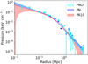 |
Fig. 1. Pressure profiles derived from the full 150 GHz map (cyan, PNO, cyan) and excluding the over-pressure region (PN, blue). The dots and error bars correspond to the non-parametric fit to the SZ. The shadow region represents the best-fit gNFW model to the non-parametric pressure profiles. We also show in red the universal pressure profile (Arnaud et al. 2010) for the cluster (PA10). |
In summary, we consider in this work three tSZ-based estimates of the ICM thermal pressure profile of MACS J0647.7+7015: (1) a NIKA2-Planck combined analysis including the over-pressure region (PNO), (2) a NIKA2-Planck combined analysis excluding the over-pressure region (PN), and (3): the universal pressure profile (PA10; Arnaud et al. 2010). The last, which is also presented in Fig. 1, was obtained by fitting a gNFW model to the data with the slope parameters a, b, and c fixed to the universal pressure profile values (Arnaud et al. 2010) and P0 and rp as free parameters.
2.2. X-ray-based electron density and pressure profiles
Deep X-ray observations of MACS J0647.7+7015 by XMM-Newton (effective exposure time of ∼68 ks) permit the reconstruction of both the electron density and temperature profiles, from which the pressure profile can also be determined. We used the data presented in Ruppin et al. (2018) that were processed using the standard procedures presented, for example, in Bartalucci et al. (2017). We notice that, as shown by Ruppin et al. (2018), no significant over-density region was identified in the southwest region of MACS J0647.7+7015 in the XMM-Newton X-ray surface brightness map. However, we considered two estimates of the electron density radial profile obtained by excluding or not the over-pressure region. The former was already presented in Ruppin et al. (2018). In both cases, the same procedure was used to constrain the gas density profile from the XMM-Newton observations, and it is described in detail in Pratt et al. (2010) and Planck Collaboration Int. III (2013).
The deprojected gas density profiles were fitted by a simplified Vikhlinin et al. (2006) parametric model given by
![Mathematical equation: $$ \begin{aligned} n_{\rm e}(r) = n_{\rm e0} \left[1+\left(\frac{r}{r_{\rm c}}\right)^2\right]^{-3 \beta /2} \left[1+\left(\frac{r}{r_{\rm s}}\right)^{\gamma }\right]^{-\epsilon /2\gamma }, \end{aligned} $$](/articles/aa/full_html/2022/05/aa40276-21/aa40276-21-eq1.gif) (1)
(1)
where ne0 is the central gas density, rc is the core radius, and rs is the transition radius at which an additional steepening in the profile occurs. The β and ϵ parameters define the inner and the outer profile slopes, respectively. The γ parameter gives the width of the transition in the profile. The value of the γ parameter was fixed to 3 since it provides a good description of all the clusters considered in the analysis of Vikhlinin (2006).
The XMM-Newton data can also be used to estimate the cluster pressure profile by combining the gas density profiles discussed above and the gas temperature determined from the spectroscopic observations via a deprojection procedure as presented in Pratt et al. (2010) and Planck Collaboration Int. III (2013). We used two X-ray-based thermal pressure profile estimates for MACS J0647.7+7015: (1) including the over-pressure region (PXO) and (2) excluding the over-pressure region (PX). The latter was already presented in Ruppin et al. (2018). These two pressure profiles allow us to assess the consistency between the X-ray and tSZ views of the ICM. We show in the top row of Fig. 2 the electronic density and temperature as directly derived from the XMM-Newton data set. The dark and light green dots (and error bars) correspond to the profiles derived from the full cluster data and excluding the over-pressure, respectively. In the bottom row we show the derived pressure profile with the same color scheme. It should be noted that in this analysis we are limited by the extension of the temperature profile, which can be computed up to about 1.3 Mpc (full data) and 1 Mpc (excluding over-pressure). In the following, the hydrostatic mass profile for the X-ray-only results are extrapolated linearly beyond this radius.
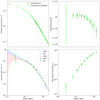 |
Fig. 2. Electron density, temperature, pressure, and hydrostatic mass profiles as derived from the XMM-Newton X-ray data. The dark and light green dots represent the profile computed using the full cluster emission and masking the over-pressure area, respectively. We also show for comparison the PN, PNO, and PA10 pressure profiles presented in Fig. 1. |
2.3. Estimation of the hydrostatic mass profile
Assuming HE, the total mass enclosed within the radius r is given by
 (2)
(2)
where G is the gravitational constant, mp the proton mass, μgas = 0.61 the mean molecular weight of the gas, and ne and Pe the cluster gas electron density and pressure radial profiles.
The hydrostatic mass profile of MACS J0647.7+7015 computed using Eq. (2) is shown in Fig. 3 for the five pressure profiles discussed above: PN, PNO, PA10, PX, and PXO. In terms of electron density, we used the electron density profiles discussed above including (in combination with PNO, PA10, and PXO) or excluding (in combination with PN and PX) the over-pressure region. As discussed above, the extension of the hydrostatic mass profiles for the X-ray-only estimate was limited by the temperature profiles, and they were then extrapolated linearly beyond 1.3 Mpc and 1 Mpc for the analysis, including and excluding the over-pressure region, respectively. To derive the combined X-ray and tSZ hydrostatic mass profiles, the non-parametric pressure estimates were previously fitted to a gNFW model (see Fig. 1), and estimates of the pressure derivative were obtained from the best-fit models.
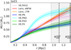 |
Fig. 3. Combined X-ray and tSZ hydrostatic mass profile computed using three different electron pressure estimates: (1) non-parametric fit using the full 150 GHz NIKA2 map (HE over-pressure, PNO, cyan), (2) non-parametric fit masking the over-pressure region (HE, PN, blue), and (3) the universal Arnaud et al. (2010) pressure profile for this cluster (pink, PA10). Also shown are reconstructed X-ray-only hydrostatic mass profiles, excluding (PX, dark green) and including over-pressure (PXO, bright green), as well as a reconstructed lensing mass profile for the eNFW (red) and LTM models (orange). The vertical dotted line represents the maximum radius at which the lensing data are available. The dashed lines show the characteristic radii |


We observe significant differences between the three tSZ- and X-ray-based estimates (for PN, PNO, and PA10), even at the large radii at which the cluster masses are traditionally given in the literature, R500 and R200. We remind the reader that when including the over-pressure region the tSZ data are significantly not circularly symmetric, thus breaking the hypothesis made for the computation of the pressure and hydrostatic mass profiles. In addition, we find that the two X-ray-only-based estimates (for PXO and PX) are consistent with each other and with the PN-based estimate. The over-pressure does not seem to affect the measured X-ray brightness.
We present in Table 1 estimates of the characteristic radius,  , and of the hydrostatic mass at this radius,
  , for the PN, PNO, and PA10 pressure profiles. We notice that the estimates for the PXO and PX pressure profiles are consistent with those of the PN one. We observe in the table that there are significant differences in the estimate of the characteristic mass and the radius, which are either related to the over-pressure region or to the differences in the modeling of the pressure profile. These mass estimates can also be compared to results in the literature based on integrated quantities as
  based on L500 (Piffaretti et al. 2011) and
  based on YSZ (Planck Collaboration XXVII 2016). Although here we only present results for a single cluster, these differences in the mass estimates are illustrative of the systematic uncertainties one would encounter when deriving the hydrostatic mass of a cluster for which we do not have high resolution observations. These uncertainties need to be accounted for when deriving scaling relations relating the cluster integrated observables (Y500 and
  ) to the hydrostatic mass. In the following, we define
  as the characteristic radius,
  , for the PN pressure profile estimate and use it for comparison with the lensing estimate discussed in Sect. 3.
R500 and M500 as derived from the hydrostatic mass profiles for the PN, PNO, PA10, PXO, and PX pressure profile estimates.
3. Lensing mass density profile
In this section we discuss the reconstruction of the lensing mass density profile of MACS J0647.7+7015 using data from the Hubble Space Telescope (Postman et al. 2012).
3.1. Data and preprocessing
Our analysis is based on the joint weak and strong lensing convergence map (hereafter κ-map) of MACS J0647.7+7015 obtained by Zitrin et al. (2015) in their study of the 25 CLASH clusters (Postman et al. 2012). In Zitrin et al. (2015) the authors considered two different parametrizations for the lens model: (1) a light-trace-mass (LTM) density profile and (2) a pseudo isothermal elliptical mass distribution plus an elliptical Navarro-Frenk-White (PIEMD+eNFW) density profile (Navarro et al. 1996). More details on these two approaches can be found in Zitrin et al. (2009, 2013a,b, 2015). Although we considered both parametrizations, we limit our presentation here to the analysis of the κ-map corresponding to the second approach as we find equivalent results. The PIEMD+eNFW κ-map of MACS J0647.7+7015 delivered by Zitrin et al. (2015) exhibits an elliptical morphology, with a somewhat larger ellipticity than the tSZ NIKA2 map of the cluster, and with the major axis pointing slightly northward.
The convergence, κ, is a measure of the projected mass density per unit of critical density at sky position θ:
 (3)
(3)
with
 (4)
(4)
where Dl, Ds, and Dls are the angular diameter distance between, respectively, the observer and the lens, the observer and the source, and the source and the lens. The θ is the 2D angular separation with respect to the cluster center.
Using Eqs. (3) and (4), and assuming that the background sources are at a redshift of zs = 2 (Zitrin et al. 2011, 2015), we can directly compute the projected mass density profile, Σ(r), from the κ-map by averaging the signal in rings of increasing distance from the center of the cluster, which is taken to be the same as the center used in the hydrostatic mass analysis. In the left panel of Fig. 4 we show the projected mass density profile obtained by averaging the PIEMD+eNFW κ-map within 60 rings logarithmically spaced up to a distance from the center of the cluster of 2.3 arcmin, corresponding to a physical radius of R ∼ 1 Mpc (black points). The uncertainties in the projected mass density profile are computed from the standard deviation in each bin in order to account, to first order, for the observed ellipticity in the PIEMD+eNFW κ-map.
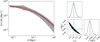 |
Fig. 4. Lensing analysis. Left: projected lensing mass density profile as a function of radius from the PIEMD+eNFW κ-map Zitrin et al. (2015) lens model (black points). Also shown are our best-fit projected NFW profile and 1σ uncertainties (red line and shaded area). The 2D sky angular separation from the cluster center has been converted to radial distance (in Mpc) using the angular distance at the cluster redshift. Right: 2D and 1D posterior probability distributions for the c200 and rs parameters of the 3D mass profile as obtained from the MCMC analysis. |
3.2. Three-dimensional mass profile reconstruction
From the projected lensing mass density we can reconstruct the 3D density profile of the cluster, which we parametrize by using a 3D Navarro-Frenk-White (NFW; Navarro et al. 1996) density profile. Assuming spherical symmetry for the cluster, and using Eqs. (7)–(9) from Bartelmann (1996), the projected 3D NFW density profile is given by
 (5)
(5)
as a function of the NFW model parameters ρs and rs, where x = r/rs and ρs = δc ρc. We define
 (6)
(6)
where c200 = r200/rs is the concentration parameter and ρc the critical density of the Universe.
We fitted the numerical projected mass density profile from Fig. 4 to the model in Eq. (5) using as free parameters the characteristic cluster radius, rs, and the concentration parameter, c200. We performed an MCMC analysis to obtain the best-fit parameters. In particular, we used the emcee MCMC software implemented in Python by Foreman-Mackey et al. (2013) and Goodman & Weare (2010). We ran the MCMC code using 100 walkers until the convergence criteria proposed by Gelman & Rubin (1992) were fulfilled for all the model parameters. The 2D and 1D posterior probability distributions for rs and c200 are shown in the right panel of Fig. 4. The marginalized best-fit values are rs = 0.56 ± 0.07 Mpc and c200 = 3.68 ± 0.29. For comparison, we also show in the left panel of Fig. 4 our best-fit model, including 1σ uncertainties.
Using these best-fit parameters and uncertainties, we computed the lensing mass profile of MACS J0647.7+7015, which we display in Fig. 3. For illustration, the corresponding  kpc is shown. We also find
  kpc. From the mass profile we obtain
  and the virial mass
  . We notice that from the analysis of the LTM κ-map we find slightly larger masses, but they are consistent within uncertainties:
  . Combining the two estimates we obtain
  . We assumed that the difference between the two models is a good representation of the modeling’s systematic uncertainties. The derived lensing masses are consistent with the one obtained by Umetsu et al. (2014),
  ; in their analysis they combined the strong and weak lensing constraints of a fraction of 20 CLASH clusters and fitted a stacked density profile.
However, our best-fit value of the concentration parameter is more than 2σ larger than theirs. Similar conclusions can be drawn from the comparison to the results recently obtained by Umetsu et al. (2018), who found  = (11.73 ± 3.79) × 1014 M⊙ using an eNFW model.
We observe that there is good consistency between the different lensing mass estimates. However, we must stress here the fact that numerical simulations indicate that lensing mass estimates may be affected by systematic uncertainties (see Pratt et al. 2019, for a review). Among them, the uncertainties induced by the mass modeling are probably well represented by the scatter within the different estimates presented here. On the contrary, others, such as those induced by the uncertainties on the redshift and shape of the cluster galaxies and on the choice of background galaxies, are difficult to estimate for the data used in this paper.
4. Discussion
4.1. Gas to lensing mass fraction
From the electron density profile described in Sect. 2.2 we can compute the gas mass profile. Using the lensing mass profile, we computed the gas to lensing mass fraction  , which is presented in Fig. 5 as a function of the normalized radius, assuming
  as a reference. As neither the electron density nor the lensing mass profile estimates reach large radii, we believe that the steep increase in the gas fraction observed at those radii is most probably due to a computational artifact. Uncertainties at the 1σ level are shown. We find that at
  the gas fraction is fgas = 0.084 ± 0.009. This value is compatible with the results of Pratt et al. (2016) from an X-ray analysis. It is also marginally in agreement with the results found from the MUSIC hydro-dynamical simulations (Sembolini et al. 2013), the results obtained by Chiu et al. (2018) from their analyses of 91 South Pole Telescope selected clusters, and the results of Planck Collaboration Int. V (2013) on intermediate and low redshift clusters.
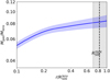 |
Fig. 5. Gas to lensing mass fraction and uncertainties (blue line and violet shaded area). |
Furthermore, by assuming a stellar fraction of ∼6% (Chiu et al. 2018) and that the lensing mass estimate is a good proxy for the total mass of the cluster, the resulting baryon fraction is in agreement with the one from Planck Collaboration VI (2020).
4.2. Comparison of the hydrostatic and lensing mass profiles
In Fig. 3 we directly compare the five estimates of the hydrostatic mass profiles and the lensing mass profiles derived in Sects. 2.3 and 3. We can observe significant differences between these profiles. We see that in the case of the joint tSZ and X-ray estimates, the over-pressure region significantly increases the hydrostatic mass profile estimate (HE, PNO), as discussed in Ruppin et al. (2018). Such an increase results in a larger cluster hydrostatic mass for a given fixed characteristic cluster radius. The estimate of M500 from the lensing analysis is smaller but is consistent with the one from the hydrostatic analysis when including the over-pressure (HE, PNO), and nearly a factor of two larger than the one obtained when excluding the over-pressure (HE,PN). They are also a factor of two larger than the ones obtained from the X-ray-only estimates, both excluding (HE, PX) and including (HE, PXO) the over-pressure region.
In Fig. 3 we also show the cluster characteristic radius as computed from the hydrostatic mass profile excluding the over-pressure region (HE, PN),  , and the one derived from the lensing mass profile,
  . We observe that the two estimates are significantly different.
The effects discussed above add an extra layer of complexity to the cosmological use of the hydrostatic mass estimates. They show that in practice: (1) the estimates of R500 and, as a consequence, M500 may vary significantly, and (2) the details of the dynamical state of the cluster significantly modify the estimates of the cluster properties and their inter-comparison between different cluster observables. The consequences of the presence of the over-pressure are very different on the hydrostatic mass estimates derived from the tSZ and X-ray joint analysis and from the X-ray-only analysis. The study of these systematic effects cannot rely on a single cluster and must be undertaken on a representative sample of clusters. This is one of the major scientific goals of the NIKA2 LPSZ (Mayet et al. 2020; Macias-Pérez et al. 2017).
4.3. Hydrostatic to lensing mass bias
From the results on the gas to lensing mass fraction, it seems that the lensing mass might be a good estimate of the total mass of the cluster. Therefore, it is interesting to infer a hydrostatic to lensing mass bias. In Fig. 6 we show the ratio between the hydrostatic mass profile and the lensing mass profile for the five pressure profile estimates discussed in Sect. 2. We observe that the MHE/Mlens ratio varies from the inner part of the cluster to the outskirts. In particular, we find a clear peak for the three hydrostatic mass profile estimates based on the joint tSZ and X-ray analysis, which is probably due to the sharp change in slope that biases toward larger values of the hydrostatic mass in the inner part of the cluster. Significant gradients are also observed in the MHE/Mlens ratio between  and
and  , but it becomes constant at very large radii, typically on the order of R200. We note that for these large radii the lensing mass profile is not directly measured but is extrapolated from the best-fit model.
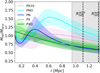 |
Fig. 6. Hydrostatic to lensing mass ratio for the hydrostatic mass profile estimates for the different pressure profile estimates presented in Sect. 2.3. Uncertainties at the 1σ level are shown as shaded areas of the corresponding color. |
We computed the hydrostatic to lensing mass bias from the MHE/Mlens ratio for a given characteristic radius, R500. We defined it as  following the notation in Planck Collaboration XX (2014), Planck Collaboration XXII (2016) for the hydrostatic mass bias. Building on the discussion presented in the previous section, we expect this value to vary significantly for the different estimates of the hydrostatic mass. As the estimates of R500 vary significantly, and to further illustrate the possible systematic uncertainties in cosmological analyses, we computed this hydrostatic to lensing mass bias for the two estimates of the characteristic radius, R500, discussed above:
  and
and  . The main results are given in Table 2. We observe in the table that the hydrostatic to lensing mass bias varies significantly, undergoing both positive and negative bias. These differences are mainly due to the differences in the hydrostatic mass profiles discussed above. However, we also stress the fact that to compute the hydrostatic to lensing mass bias, a common choice of the characteristic radius has to be made, and this can introduce further systematic uncertainties. In Table 2 we observe that for this cluster the hydrostatic to lensing mass bias is consistent within uncertainties for the two extreme choices of the characteristic radius, R500.
Hydrostatic to lensing mass bias, BHE − lens, computed from the ratio of the hydrostatic and lensing mass profiles.
5. Summary and conclusions
We have presented in this paper a high resolution multiwavelength analysis of the cluster of galaxies MACS J0647.7+7015. This analysis is a pilot study for the exploitation of the cluster sample from the NIKA2 LPSZ, which will consist of a sample of 45 clusters (24 of which have been already observed) with redshift ranging from 0.5 to 0.9 and expected masses, M500, from 1014 to 1015 M⊙.
We have used high and low resolution tSZ observations from the NIKA2 (Ruppin et al. 2018) and Planck (Planck Collaboration XXII 2016) experiments, X-ray data from the XMM-Newton satellite, and the lensing reconstruction obtained from the Hubble Space Telescope CLASH project (Zitrin et al. 2015). From the projected observables and using MCMC techniques, we have been able to derive to high accuracy the 3D hydrostatic and lensing mass profiles beyond the R500 characteristic radius of the cluster. Following the analysis of Ruppin et al. (2018), we computed the hydrostatic mass profile including and excluding the over-pressure region that they identified for different combinations of the tSZ and X-ray data and for the universal profile model (Arnaud et al. 2010). We find significant differences between the different estimates of the hydrostatic mass. These differences are related to the assumptions on the dynamical state of the cluster (including or excluding the over-pressure region), the observables used (tSZ and X-ray joint analysis versus X-ray-only analysis), and the pressure profile models considered.
From the comparison of the hydrostatic and lensing mass profiles of MACS J0647.7+7015 we discuss systematic uncertainties in the estimates of the characteristic quantities that represent the cluster, such as the characteristic radius (R500), the hydrostatic and lensing masses ( and
and  ) at that radius, their ratio, and the gas fraction. We find that the hydrostatic mass estimates, M500, at the characteristic radius, R500, vary by factors of up to two depending on the dynamical state of the cluster (including or excluding the over-pressure region), the choice of the data used (combined tSZ and X-ray versus X-ray-only analyses), and the pressure profile estimate. We also find that the hydrostatic mass estimates are, as expected, smaller overall than those obtained from the lensing mass profile but for the joint tSZ and X-ray analysis when the over-pressure is considered. Equivalently, the estimates of R500 vary by up to 30%. This makes the comparison between different mass estimates given in the literature difficult if no high resolution mass profiles are available. Moreover, these variations can lead to important systematics in the scaling relations used for cosmological analyses and should be accounted for.
We also computed the MACS J0647.7+7015 gas to lensing fraction at a fixed characteristic radius, R500, and find that it is in a marginal agreement with the results of Planck Collaboration Int. V (2013) on intermediate and low redshift clusters. However, by assuming that the lensing mass is a good proxy for the total mass of the cluster and assuming a stellar fraction of ∼6%, the resulting baryon fraction is compatible with the cosmic one (Planck Collaboration VI 2020).
Finally, we conclude that the above results demonstrate the need for detailed multiwavelength high resolution observations of a representative cluster sample at high redshift, as expected from the NIKA2 LPSZ, in order to fully characterize the mass-observable scaling relations used in cosmological cluster analyses.
Acknowledgments
We thank M. Arnaud, C. Combet and G. Pratt for very useful comments and discussions. This work has been funded by the European Union’s Horizon 2020 research and innovation program under grant agreement number 687312. V.P. also acknowledges support from the European Research Council under the European Union’s Horizon 2020 research and innovation program, under grant agreement No 771282. We also acknowledge funding from the ENIGMASS French LabEx (F.R.).
References
- Abbott, T. M. C., Aguena, M., Alarcon, A., et al. 2020, Phys. Rev. D, 102, 023509 [Google Scholar]
- Adam, R., Adane, A., Ade, P. A. R., et al. 2018, A&A, 609, A115 [NASA ADS] [CrossRef] [EDP Sciences] [Google Scholar]
- Allen, S. W., Evrard, A. E., & Mantz, A. B. 2011, ARA&A, 49, 409 [Google Scholar]
- Arnaud, M., Pratt, G. W., Piffaretti, R., et al. 2010, A&A, 517, A92 [CrossRef] [EDP Sciences] [Google Scholar]
- Bahcall, N. A. 1977, ARA&A, 15, 505 [Google Scholar]
- Bartalucci, I., Arnaud, M., Pratt, G. W., et al. 2017, A&A, 608, A88 [NASA ADS] [CrossRef] [EDP Sciences] [Google Scholar]
- Bartelmann, M. 1996, A&A, 313, 697 [NASA ADS] [Google Scholar]
- Bartelmann, M. 2010, Class. Quant. Grav., 27, 233001 [CrossRef] [Google Scholar]
- Bocquet, S., Dietrich, J. P., Schrabback, T., et al. 2019, ApJ, 878, 55 [Google Scholar]
- Böhringer, H., & Chon, G. 2015, A&A, 574, L8 [NASA ADS] [CrossRef] [EDP Sciences] [Google Scholar]
- Böhringer, H., & Werner, N. 2010, A&ARv, 18, 127 [Google Scholar]
- Böhringer, H., Chon, G., Retzlaff, J., et al. 2017, AJ, 153, 220 [Google Scholar]
- Bolliet, B., Comis, B., Komatsu, E., & Macías-Pérez, J. F. 2018, MNRAS, 477, 4957 [NASA ADS] [CrossRef] [Google Scholar]
- Calvo, M., Benoît, A., Catalano, A., et al. 2016, J. Low Temp. Phys., 184, 816 [CrossRef] [Google Scholar]
- Chiu, I., Mohr, J. J., McDonald, M., et al. 2018, MNRAS, 478, 3072 [Google Scholar]
- Costanzi, M., Rozo, E., Simet, M., et al. 2019, MNRAS, 488, 4779 [NASA ADS] [CrossRef] [Google Scholar]
- de Haan, T., Benson, B. A., Bleem, L. E., et al. 2016, ApJ, 832, 95 [NASA ADS] [CrossRef] [Google Scholar]
- De Petris, M., Ruppin, F., Sembolini, F., et al. 2020, Eur. Phys. J. Web Conf., 228, 00008 [CrossRef] [EDP Sciences] [Google Scholar]
- Foreman-Mackey, D., Conley, A., Meierjurgen Farr, W., et al. 2013, Astrophysics Source Code Library [record ascl:1303.002] [Google Scholar]
- Gelman, A., & Rubin, D. B. 1992, Stat. Sci., 7, 457 [Google Scholar]
- Gianfagna, G., De Petris, M., Yepes, G., et al. 2021, MNRAS, 502, 5115 [NASA ADS] [CrossRef] [Google Scholar]
- Goodman, J., & Weare, J. 2010, Commun. Appl. Math. Comput. Sci., 5, 65 [Google Scholar]
- Kravtsov, A. V., & Borgani, S. 2012, ARA&A, 50, 353 [Google Scholar]
- Macias-Pérez, J. F., Adam, R., Ade, P., et al. 2017, Proceedings of the European Physical Society Conference on High Energy Physics, 42 [Google Scholar]
- Mayet, F., Adam, R., Ade, P., et al. 2020, Eur. Phys. J. Web Conf., 228, 00017 [Google Scholar]
- Nagai, D., Kravtsov, A. V., & Vikhlinin, A. 2007, ApJ, 668, 1 [Google Scholar]
- Navarro, J. F., Frenk, C. S., & White, S. D. M. 1996, ApJ, 462, 563 [Google Scholar]
- Pacaud, F., Pierre, M., Melin, J. B., et al. 2018, A&A, 620, A10 [NASA ADS] [CrossRef] [EDP Sciences] [Google Scholar]
- Perotto, L., Ponthieu, N., Macías-Pérez, J. F., et al. 2020, A&A, 637, A71 [NASA ADS] [CrossRef] [EDP Sciences] [Google Scholar]
- Piffaretti, R., Arnaud, M., Pratt, G. W., Pointecouteau, E., & Melin, J. B. 2011, A&A, 534, A109 [NASA ADS] [CrossRef] [EDP Sciences] [Google Scholar]
- Planck Collaboration XX. 2014, A&A, 571, A20 [NASA ADS] [CrossRef] [EDP Sciences] [Google Scholar]
- Planck Collaboration XXI. 2014, A&A, 571, A21 [NASA ADS] [CrossRef] [EDP Sciences] [Google Scholar]
- Planck Collaboration XXII. 2016, A&A, 594, A22 [NASA ADS] [CrossRef] [EDP Sciences] [Google Scholar]
- Planck Collaboration XXIV. 2016, A&A, 594, A24 [NASA ADS] [CrossRef] [EDP Sciences] [Google Scholar]
- Planck Collaboration XXVII. 2016, A&A, 594, A27 [NASA ADS] [CrossRef] [EDP Sciences] [Google Scholar]
- Planck Collaboration I. 2020, A&A, 641, A1 [NASA ADS] [CrossRef] [EDP Sciences] [Google Scholar]
- Planck Collaboration VI. 2020, A&A, 641, A6 [NASA ADS] [CrossRef] [EDP Sciences] [Google Scholar]
- Planck Collaboration Int. III. 2013, A&A, 550, A129 [NASA ADS] [CrossRef] [EDP Sciences] [Google Scholar]
- Planck Collaboration Int. V. 2013, A&A, 550, A131 [NASA ADS] [CrossRef] [EDP Sciences] [Google Scholar]
- Planck Collaboration Int. XI. 2013, A&A, 557, A52 [NASA ADS] [CrossRef] [EDP Sciences] [Google Scholar]
- Postman, M., Coe, D., Benítez, N., et al. 2012, ApJS, 199, 25 [Google Scholar]
- Pratt, G. W., Arnaud, M., Piffaretti, R., et al. 2010, A&A, 511, A85 [NASA ADS] [CrossRef] [EDP Sciences] [Google Scholar]
- Pratt, G. W., Pointecouteau, E., Arnaud, M., & van der Burg, R. F. J. 2016, A&A, 590, L1 [NASA ADS] [CrossRef] [EDP Sciences] [Google Scholar]
- Pratt, G. W., Arnaud, M., Biviano, A., et al. 2019, Space Sci. Rev., 215, 25 [Google Scholar]
- Ruppin, F., Adam, R., Comis, B., et al. 2017, A&A, 597, A110 [NASA ADS] [CrossRef] [EDP Sciences] [Google Scholar]
- Ruppin, F., Mayet, F., Pratt, G. W., et al. 2018, A&A, 615, A112 [NASA ADS] [CrossRef] [EDP Sciences] [Google Scholar]
- Ruppin, F., Mayet, F., Macías-Pérez, J. F., & Perotto, L. 2019a, MNRAS, 490, 784 [NASA ADS] [CrossRef] [Google Scholar]
- Ruppin, F., Sembolini, F., De Petris, M., et al. 2019b, A&A, 631, A21 [NASA ADS] [CrossRef] [EDP Sciences] [Google Scholar]
- Salvati, L., Douspis, M., Ritz, A., Aghanim, N., & Babul, A. 2019, A&A, 626, A27 [NASA ADS] [CrossRef] [EDP Sciences] [Google Scholar]
- Salvati, L., Douspis, M., & Aghanim, N. 2020, A&A, 643, A20 [NASA ADS] [CrossRef] [EDP Sciences] [Google Scholar]
- Sarazin, C. L. 1988, X-ray Emission from Clusters of Galaxies (Cambridge: Cambridge University Press) [Google Scholar]
- Sembolini, F., Yepes, G., De Petris, M., et al. 2013, MNRAS, 429, 323 [NASA ADS] [CrossRef] [Google Scholar]
- Sunyaev, R. A., & Zel’dovich, Y. B. 1972, Astrophys. Space Phys. Res., 4, 173 [Google Scholar]
- Sunyaev, R. A., & Zel’dovich, Y. B. 1980, ARA&A, 18, 537 [NASA ADS] [CrossRef] [Google Scholar]
- Umetsu, K., Medezinski, E., Nonino, M., et al. 2014, ApJ, 795, 163 [NASA ADS] [CrossRef] [Google Scholar]
- Umetsu, K., Sereno, M., Tam, S.-I., et al. 2018, ApJ, 860, 104 [Google Scholar]
- Vikhlinin, A. 2006, ApJ, 640, 710 [NASA ADS] [CrossRef] [Google Scholar]
- Vikhlinin, A., Kravtsov, A., Forman, W., et al. 2006, ApJ, 640, 691 [Google Scholar]
- Zitrin, A., Broadhurst, T., Umetsu, K., et al. 2009, MNRAS, 396, 1985 [NASA ADS] [CrossRef] [Google Scholar]
- Zitrin, A., Broadhurst, T., Barkana, R., Rephaeli, Y., & Benítez, N. 2011, MNRAS, 410, 1939 [NASA ADS] [Google Scholar]
- Zitrin, A., Menanteau, F., Hughes, J. P., et al. 2013a, ApJ, 770, L15 [NASA ADS] [CrossRef] [Google Scholar]
- Zitrin, A., Meneghetti, M., Umetsu, K., et al. 2013b, ApJ, 762, L30 [NASA ADS] [CrossRef] [Google Scholar]
- Zitrin, A., Fabris, A., Merten, J., et al. 2015, ApJ, 801, 44 [Google Scholar]
All Tables
R500 and M500 as derived from the hydrostatic mass profiles for the PN, PNO, PA10, PXO, and PX pressure profile estimates.
Hydrostatic to lensing mass bias, BHE − lens, computed from the ratio of the hydrostatic and lensing mass profiles.
All Figures
|
Fig. 1. Pressure profiles derived from the full 150 GHz map (cyan, PNO, cyan) and excluding the over-pressure region (PN, blue). The dots and error bars correspond to the non-parametric fit to the SZ. The shadow region represents the best-fit gNFW model to the non-parametric pressure profiles. We also show in red the universal pressure profile (Arnaud et al. 2010) for the cluster (PA10). |
| In the text | |
|
Fig. 2. Electron density, temperature, pressure, and hydrostatic mass profiles as derived from the XMM-Newton X-ray data. The dark and light green dots represent the profile computed using the full cluster emission and masking the over-pressure area, respectively. We also show for comparison the PN, PNO, and PA10 pressure profiles presented in Fig. 1. |
| In the text | |
|
Fig. 3. Combined X-ray and tSZ hydrostatic mass profile computed using three different electron pressure estimates: (1) non-parametric fit using the full 150 GHz NIKA2 map (HE over-pressure, PNO, cyan), (2) non-parametric fit masking the over-pressure region (HE, PN, blue), and (3) the universal Arnaud et al. (2010) pressure profile for this cluster (pink, PA10). Also shown are reconstructed X-ray-only hydrostatic mass profiles, excluding (PX, dark green) and including over-pressure (PXO, bright green), as well as a reconstructed lensing mass profile for the eNFW (red) and LTM models (orange). The vertical dotted line represents the maximum radius at which the lensing data are available. The dashed lines show the characteristic radii |
| In the text | |
|
Fig. 4. Lensing analysis. Left: projected lensing mass density profile as a function of radius from the PIEMD+eNFW κ-map Zitrin et al. (2015) lens model (black points). Also shown are our best-fit projected NFW profile and 1σ uncertainties (red line and shaded area). The 2D sky angular separation from the cluster center has been converted to radial distance (in Mpc) using the angular distance at the cluster redshift. Right: 2D and 1D posterior probability distributions for the c200 and rs parameters of the 3D mass profile as obtained from the MCMC analysis. |
| In the text | |
|
Fig. 5. Gas to lensing mass fraction and uncertainties (blue line and violet shaded area). |
| In the text | |
|
Fig. 6. Hydrostatic to lensing mass ratio for the hydrostatic mass profile estimates for the different pressure profile estimates presented in Sect. 2.3. Uncertainties at the 1σ level are shown as shaded areas of the corresponding color. |
| In the text | |
Current usage metrics show cumulative count of Article Views (full-text article views including HTML views, PDF and ePub downloads, according to the available data) and Abstracts Views on Vision4Press platform.
Data correspond to usage on the plateform after 2015. The current usage metrics is available 48-96 hours after online publication and is updated daily on week days.
Initial download of the metrics may take a while.