| Issue |
A&A
Volume 660, April 2022
|
|
|---|---|---|
| Article Number | A69 | |
| Number of page(s) | 25 | |
| Section | Extragalactic astronomy | |
| DOI | https://doi.org/10.1051/0004-6361/202142627 | |
| Published online | 13 April 2022 | |
Stellar masses, sizes, and radial profiles for 465 nearby early-type galaxies: An extension to the Spitzer survey of stellar structure in Galaxies (S4G)⋆
1
Space Physics and Astronomy Research Unit, University of Oulu, Oulu 90014, Finland
e-mail: a.emery.watkins@gmail.com
2
Centre for Astrophysics Research, School of Physics, Astronomy and Mathematics, University of Hertfordshire, Hatfield AL10 9AB, UK
3
Astrophysics Research Institute, Liverpool John Moores University, IC2, Liverpool Science Park, 146 Brownlow Hill, Liverpool L3 5RF, UK
4
Finnish Centre of Astronomy with ESO (FINCA), University of Turku, Vesilinnantie 5, 20014 Turku, Finland
5
Specim, Spectral Imaging Ltd., Elektroniikkatie 13, 90590 Oulu, Finland
6
Departamento de Astrofísica, Universidad de La Laguna, 38200 La Laguna, Tenerife, Spain
7
Instituto de Astrofísica de Canarias, 38205 La Laguna, Tenerife, Spain
8
Department for Physics, Engineering Physics and Astrophysics, Queen’s University, Kingston, ON K7L 3N6, Canada
9
Department of Physics and Astronomy, University of Alabama, Box 870324, Tuscaloosa, AL 35487, USA
10
Aix Marseille Univ, CNRS, CNES, LAM, Marseille, France
11
Kavli Institute for Astronomy and Astrophysics, Peking University, Beijing 100871, PR China
12
Department of Astronomy, School of Physics, Peking University, Beijing 100871, PR China
13
University of Louisville, Department of Physics and Astronomy, 102 Natural Science Building, 40292 KY, Louisville, USA
14
Department of Astronomy and Atmospheric Sciences, Kyungpook National University, Daegu 41566, Korea
15
IPAC, Mail Code 314-6, Caltech, 1200 E. California Blvd., Pasadena, CA 91125, USA
16
Valongo Observatory, Federal University of Rio de Janeiro, Ladeira Pedro Antônio, 43, Saúde CEP, 20080-090 Rio de Janeiro, RJ, Brazil
17
Kapteyn Astronomical Institute, University of Groningen, PO Box 800, 9700 AV Groningen, The Netherlands
18
NASA Headquarters Mary W. Jackson Building, 300 E Street SW, Washington, DC 20546, USA
19
Steward Observatory and Department of Astronomy, University of Arizona, 933 N. Cherry Ave., Tucson, AZ 85721, USA
Received:
9
November
2021
Accepted:
18
January
2022
Context. The Spitzer Survey of Stellar Structure in Galaxies (S4G) is a detailed study of over 2300 nearby galaxies in the near-infrared (NIR), which has been critical to our understanding of the detailed structures of nearby galaxies. Because the sample galaxies were selected only using radio-derived velocities, however, the survey favored late-type disk galaxies over lenticulars and ellipticals.
Aims. A follow-up Spitzer survey was conducted to rectify this bias, adding 465 early-type galaxies (ETGs) to the original sample, to be analyzed in a manner consistent with the initial survey. We present the data release of this ETG extension, up to the third data processing pipeline (P3): surface photometry.
Methods. We produce curves of growth and radial surface brightness profiles (with and without inclination corrections) using reduced and masked Spitzer IRAC 3.6 μm and 4.5 μm images produced through Pipelines 1 and 2, respectively. From these profiles, we derive the following integrated quantities: total magnitudes, stellar masses, concentration parameters, and galaxy size metrics. We showcase NIR scaling relations for ETGs among these quantities.
Results. We examine general trends across the whole S4G and ETG extension among our derived parameters, highlighting differences between ETGs and late-type galaxies (LTGs). The latter are, on average, more massive and more concentrated than LTGs, and subtle distinctions are seen among ETG morphological subtypes. We also derive the following scaling relations and compare them with previous results in visible light: mass-size (both half-light and isophotal), mass-concentration, mass-surface brightness (central, effective, and within 1 kpc), and mass-color.
Conclusions. We find good agreement with previous works, though some relations (e.g., mass-central surface brightness) will require more careful multicomponent decompositions to be fully understood. The relations between mass and isophotal radius and between mass and surface brightness within 1 kpc, in particular, show notably small scatter. The former provides important constraints on the limits of size growth in galaxies, possibly related to star formation thresholds, while the latter–particularly when paired with the similarly tight relation for LTGs–showcases the striking self-similarity of galaxy cores, suggesting they evolve little over cosmic time. All of the profiles and parameters described in this paper will be provided to the community via the NASA/IPAC database on a dedicated website.
Key words: galaxies: evolution / galaxies: photometry / galaxies: elliptical and lenticular, cD / galaxies: structure / galaxies: statistics / galaxies: spiral
Full Table A.1, as well as all derived photometric properties and images (including masks and weight maps) are available at the CDS via anonymous ftp to cdsarc.u-strasbg.fr (130.79.128.5) or via http://cdsarc.u-strasbg.fr/viz-bin/cat/J/A+A/660/A69
© ESO 2022
1. Introduction
Over cosmic time, galaxies acquire and process baryons, turning into stars and redistributing those stars through interactions with neighboring systems or through their own internal gravitational processes. Under Λ cold dark matter (ΛCDM) cosmology (White & Rees 1978; Frenk et al. 1985), galaxies form via the hierarchical merging of dark matter halos, which in the early Universe served as the potential wells into which baryons initially settled. Given the hierarchical nature of the merging, the centers of galaxies likely formed first, and subsequent gas or satellite accretions (e.g., Kauffmann et al. 1993; Bendo & Barnes 2000; Aguerri et al. 2001; Balcells et al. 2003; Bournaud et al. 2007; Athanassoula et al. 2016) and secular evolution (e.g., Combes & Sanders 1981; Kormendy 1982; Fathi & Peletier 2003; Kormendy & Kennicutt 2004; Athanassoula 2005) then conspired to modify both these centers and the structures built atop them in complex collisional and dissipational interactions. Nearby galaxies display the present end results of these interactions; therefore, detailed study of the stellar structure of nearby galaxies is critical to understanding galaxy evolution.
It was to this end that the Spitzer Survey of Stellar Structure in Galaxies (S4G; Sheth et al. 2010) was carried out, providing excellent quality deep imaging of over 2300 galaxies within ∼40 Mpc, in a wavelength regime, the near-infrared (NIR), that suffers little from dust extinction (Draine & Lee 1984; Calzetti 2001) and contains few emission or absorption features (e.g., Willner et al. 1977; Tokunaga et al. 1991; Kaneda et al. 2007). Stellar mass-to-light ratios are also nearly constant across stellar populations in this wavelength regime, making this imaging a nearly direct tracer of stellar mass (e.g., Pahre et al. 2004; Jun & Im 2008; Peletier et al. 2012; Meidt et al. 2014; Driver et al. 2016). The survey has been indispensible to the study of galaxy evolution, having resulted in over one hundred published papers (e.g., Buta et al. 2010 Comerón et al. 2011; Martín-Navarro et al. 2012; Zaritsky et al. 2013; Laine et al. 2014, 2016; Herrera-Endoqui et al. 2015; Kim et al. 2016; Laurikainen & Salo 2017; Bouquin et al. 2018; Díaz-García et al. 2019; İkz et al. 2020). Yet, until now, it has suffered from a serious bias: the velocity cut in the original survey used only radio measurements, thereby excluding gas-poor–mostly early-type–galaxies.
Early-type galaxies (ETGs), being typically gas- and dust-poor and dominated by evolved stellar populations, are often referred to as “red and dead”. This is an unfortunate term, connoting a lack of interesting properties or phenomena. The term ETG–referring to the classification scheme of increasing morphological complexity proposed by Hubble (1926) – covers both the disk-dominated and rotation-supported lenticular (S0) galaxies, as well as the more pressure-supported elliptical (E) galaxies. What the exact relationship is linking these two classes with each other–and with their more gas-rich, late-type galaxy (LTG) counterparts–is a long-standing question.
For example, given their many similarities with late-type spirals (including bulge-to-total mass or light ratios, range of bulge luminosities, bar properties, and kinematics; e.g., Laurikainen et al. 2011; Cappellari et al. 2011a; Kormendy & Bender 2012), S0 galaxies may have formed from LTGs through the removal or rapid consumption of gas and dust. S0s also form a parallel morphological sequence with spirals (Spitzer & Baade 1951; van den Bergh 1976; Laurikainen et al. 2011; Cappellari et al. 2011a; Kormendy & Bender 2012), lending further credence to this idea. Detailed photometric analysis has also provided evidence linking the two disk galaxy classes; Laurikainen et al. (2010) found that the sizes and masses of bulges in both early- and late-type disk galaxies correlate strongly with those of the disk, suggesting a similar kind of concurrent evolution (see also: Kormendy & Kennicutt 2004; Aguerri et al. 2005), and disk scaling relations between S0s and LTGs also appear similar (e.g., Eliche-Moral et al. 2015).
Even if the two are evolutionarily linked, however, the precise mechanisms behind the transformation from LTG to ETG are still open to debate. Because of the relative abundance of S0s in galaxy clusters, one such long-favored mechanism is infall into dense environments (e.g., Gunn et al. 1972; Dressler 1980; Moore et al. 1996; Bekki et al. 2002). This seems to happen quite early; detailed study of nearby cluster S0 stellar populations frequently shows quenching epochs over 10 Gyr ago (e.g., Sil’chenko 2013; Comerón et al. 2016; Katkov et al. 2019). However, isolated field S0s, though rare, do exist (Karachentsev et al. 2010), ruling out cluster or group infall as the sole formation pathway. Falcón-Barroso et al. (2019) also argued that simple quenching and fading of stellar populations is unlikely to be the dominant spiral–S0 transformation mechanism given the differences in angular momentum between the classes (with simulations suggesting major mergers may instead explain these S0 kinematics; Querejeta et al. 2015), though such quenching may still occur in low-density environments (e.g., Rizzo et al. 2018). Environmental influence may not be necessary either; Saha & Cortesi (2018) showed that galaxies with properties very similar to S0s can form in isolation, via instabilities in gaseous disks. Burstein et al. (2005) also argued that the relative K-band luminosities of S0s and spirals demonstrate that direct quenching, while feasible in individual cases, may not be the dominant transformation mechanism either. Indeed, detailed comparisons between environments suggest there may be multiple quenching pathways behind the formation of S0 galaxies (e.g., Wilman & Erwin 2012). Aguerri (2012) provides a thorough review of different proposed S0 formation pathways.
The origins of elliptical galaxies, despite their relatively simple appearances, are likely equally complex. Early theories of elliptical galaxy formation relied on a monolithic collapse (Eggen et al. 1962), via either the low-rotation, dissipational collapse of gas clouds (e.g., Larson 1974a,b, 1975) or the dissipationless collapse of stars formed prior to the gas collapse time (e.g., Gott 1973, 1977; Thuan 1975). As ΛCDM cosmology came into favor, hierarchical models of elliptical galaxy formation did so as well (see the review by de Zeeuw & Franx 1991), and the discussion became more granular. The origin of elliptical galaxy rotation (or the lack thereof), for example, received a lot of focus (Bertola & Capaccioli 1975; Illingworth 1977; Binney 1978; Davies & Illingworth 1983; Wyse & Jones 1984; Barnes 1988) given its strong implications for elliptical galaxy merger histories; indeed, rotation may be critical to understanding ETG formation pathways as a whole (Cappellari 2016).
From simulations, it became clear that major mergers of gas-poor disk galaxies can result in remnants that look very much like elliptical galaxies, albeit with nearly zero net rotation (e.g., Toomre 1977; White 1983; Barnes 1988, 1990; Hernquist 1992). The prevalence of elliptical galaxies in dense environments (e.g., Oemler 1974; Dressler 1980; Cappellari et al. 2011b; Calvi et al. 2012) also points toward mergers or interactions as key formation mechanisms. Elliptical galaxies also show a diversity in their core profiles that might result from varying merger histories, with some showing continuous Sérsic profiles, while the most luminous ellipticals show central light deficits (e.g., King & Minkowski 1966; Gudehus 1973; Davies et al. 1983; Kormendy & Bender 1996; Faber et al. 1997; Ravindranath et al. 2001; Emsellem et al. 2007; Kormendy et al. 2009; Dullo & Graham 2012; Krajnović 2015; Krajnović et al. 2020, and many others). Others still show central light enhancements (e.g., Kormendy 1999; Côté et al. 2006; Kormendy et al. 2009). Core light deficits may result from scouring by supermassive black hole (SMBH) pairs (e.g., Begelman et al. 1980; Ebisuzaki et al. 1991; Milosavljević & Merritt 2001; Thomas et al. 2014) donated by merged galaxies (implying at least one major merger event), while core enhancements might occur through central starbursts induced by dissipative mergers (e.g., Mihos & Hernquist 1994; Kormendy 1999; Kormendy et al. 2009). Mergers may also be necessary to explain a seeming coupling of baryonic and dark matter kinematics in some ETGs if one assumes a constant stellar initial mass function (IMF), albeit with some dependence on local environment (Wegner et al. 2012; Corsini et al. 2017); otherwise, a nonuniversal IMF is required.
Mergers thus appear to be important for elliptical galaxy formation for most of cosmic history, but the dominant type of merger history remains ambiguous. Contrary to expectations from a major-merger formation scenario (Nipoti et al. 2003; Hopkins et al. 2008; Bezanson et al. 2009; Naab et al. 2009), mass evolution of ellipticals has been slow relative to size evolution (e.g., Trujillo et al. 2007; Buitrago et al. 2008; van Dokkum et al. 2008; Szomoru et al. 2012), and metallicity gradients in elliptical outskirts (particularly in low-luminosity ellipticals) are quite flat (e.g., Peletier et al. 1990; La Barbera et al. 2004; den Brok et al. 2011). Both indicate that, for most of cosmic history, elliptical galaxies may have grown via a complex series of minor mergers (e.g., Bournaud et al. 2007; Naab et al. 2009). Kim et al. (2012) and Ramos et al. (2015) also showed that tidal debris in their sample of ellipticals, when present, makes up only a small fraction (∼10%) of the hosts’ total mass, again implying a contribution primarily from minor mergers. Indeed, even the most well-behaved classical ellipticals show noticeable deviations from simple Sérsic profiles (e.g., Schombert 1986), suggesting perhaps a more piecemeal evolutionary history (Schombert 2015). The most massive ellipticals, however, typically show less rotational support (Cappellari et al. 2007) and more frequently have cored light deficits compared to low-mass ellipticals (Lauer et al. 2007; Kormendy et al. 2009), implying that they resulted from larger-mass-ratio mergers (though in the case of disk mergers, dissipational processes may be necessary to produce realistic kinematics in the resulting remnants; e.g., Thomas et al. 2009). Davari et al. (2017) also showed that high-redshift progenitors of massive ellipticals (red nuggets) often have surrounding disks that are mostly destroyed by z = 0.5, which should only occur under strong gravitational perturbations. Elliptical galaxy formation pathways thus seem to have a mass dependence. That said, one commonality all of these varied scenarios must reproduce is that they must somehow conspire to yield galaxies that fall on the tight scaling relation linking their structure and kinematics known as the fundamental plane (Djorgovski & Davis 1987; Dressler et al. 1987).
Given the unique contribution of ETGs to the overall picture of galaxy evolution, the S4G Team carried out an additional Spitzer survey to fill in the initial S4G’s morphological gap (S4G+, Spitzer project ID 10043; Sheth et al. 2013). To avoid confusion, as these new observations are an extension of the S4G, we hereafter refer to the full survey to date (the original S4G and the new ETG extension) as S4G+ETG. This new survey echoed the initial survey’s methodology, now targeting an additional 465 ETGs with the Spitzer Space Telescope’s (Werner et al. 2004) Infrared Array Camera (IRAC; Fazio et al. 2004) in the 3.6 μm and 4.5 μm bands. This new sample selection used the same criteria as the S4G, but rectified one of its blind spots: distance estimates based only on radio-derived redshifts, which excluded many ETGs.
With these new data in hand, we continue the S4G data processing by conducting the same photometric analyses applied to the previous 2352 S4G galaxies as part of Pipeline 3 (hereafter, P3; see Muñoz-Mateos et al. 2015, hereafter MM2015). This includes: intensity and surface brightness profiles, position angle and ellipticity profiles, total magnitudes, stellar masses, measures of central concentration, and measures of galaxy size. MM2015 provides in their Introduction a long list of the applications of this type of structural analysis, all of which remain applicable to this ETG extension sample (which includes still both disk and elliptical galaxies). This will lead into future analyses of this sample as well, including a detailed study of morphology (morphological classifications already having been completed by R. Buta, which are used throughout this paper) and multicomponent decompositions. In an era of large-scale deep surveys, most of which are primarily focused on probing large cosmic volumes (e.g., the Hyper-Suprime Cam Subaru Strategic Program, the Vera C. Rubin Observatory’s Legacy Survey of Space and Time, the Roman Space Telescope, and the Euclid Mission; Aihara et al. 2018; Ivezić et al. 2019; Spergel et al. 2015; Laureijs et al. 2010), it is critical to have a complete census of massive galaxies at redshift z = 0 for a current evolutionary end-state comparison. This is ultimately what the S4G hopes to provide.
This paper is organized as follows. In Sect.2, we discuss the S4G+ETG sample selection, observing strategy, and give a brief overview of the data reduction steps. In Sect. 3, we describe our photometric analyses. Section 4 provides an overview of the photometric parameter distributions for the entire sample, isolating ETGs for comparison. In Sect. 5, we showcase our results via a number of different scaling relations derived using the aforementioned photometric parameters. We discuss what we supply to the community and where to find it in Sect. 6, and finally provide a summary of our results in Sect. 7.
This paper presents an introduction to the S4G+ETG sample and the quantities derived from P3. Given the extraordinarily broad scope of the topic, more detailed investigations into the relations demonstrated in this paper will be published in future papers.
2. S4G ETG extension sample, observations, and data reduction
Developed by the original S4G Team, who also carried out the observations, the S4G ETG extension sample (initially denoted S4G+) followed the S4G selection criteria. This includes all galaxies in the HyperLEDA database (Paturel et al. 2003) with radial velocities v < 3000 km s−1, total extinction-corrected blue magnitudes mB, corr < 15.5, blue isophotal diameters D25 > 1 0, and Galactic latitude |b|≥30°. Previously, only radio-derived velocities were used (Sheth et al. 2010), biasing the sample toward gas-rich LTGs. To resolve this, the ETG extension included visual-band spectroscopic redshifts as well for galaxies with morphological type T ≤ 0.
We note, however, that this T-type criterion induced another previously unnoticed bias, as it excludes an additional 425 LTGs lacking radio velocity measurements. We are currently addressing this bias using ground-based i-band observations, which, due to the vastly different observing strategy and data reduction procedure, will be the subject of a future paper.
In total, S4G+ETG contains 2817 galaxies. Among these are 690 galaxies with HyperLEDA Hubble T ≤ 0, 225 of which were already present in the initial 2352 galaxy S4G sample (Muñoz-Mateos et al. 2015; Salo et al. 2015). This left an additional 465 ETGs to be subsequently observed as part of Spitzer proposal ID 10043 (Sheth et al. 2013). Among these are the following Milky Way satellites: ESO 351-30 (Sculptor Dwarf), ESO 356-4 (Fornax Dwarf), PGC 88608 (Sextans Dwarf), UGC 5470 (Leo I Dwarf), UGC 6253 (Leo II Dwarf), and UGC 10822 (Draco Dwarf). These galaxies are fully resolved into individual stars with the Spitzer IRAC resolution and hence cannot be analyzed using the surface photometry methods we describe here. Therefore, we applied the P3 procedure we describe below to 459 ETGs total, of which ∼67% and ∼33% are classified in HyperLEDA as S0s and Es, respectively. For our results and discussion, we focus on ETGs as a population, and therefore include all of the ETGs in the full S4G+ETG sample that are not MW satellites (684 in total).
We show the distribution of the HyperLEDA T-types used to select this sample in the left panel of Fig. 1, demonstrating two peaks at T = −3 (S0−) and T = −5 (E). Morphological classifications in HyperLEDA come from a compilation of sources, including indirect estimates derived from concentration indices, and hence can be somewhat unreliable. We thus derived our own morphological classifications based on the 3.6 μm images as in Buta et al. (2015), the distribution of which is shown in the rightmost panel in Fig. 1 for comparison. On closer visual inspection, not all of the ETG extension galaxies are best classified as ETGs (T > 0 for 75 galaxies in our new classifications), so, given this discrepancy, we opt to use our own classifications for the remainder of this paper in lieu of those found in HyperLEDA. We will make these new classifications available alongside all other quantities we have derived from this sample; we show a subsample of the full morphology table in the Appendix.
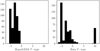 |
Fig. 1. HyperLEDA T-type distribution (left panel) and T-type distribution from 3.6 μm classifications by R. Buta (right panel) for the 465 newly observed ETGs in the S4G+ETG sample. We use the Buta T-types for the remainder of this paper, given their improved accuracy. |
The new observations mirrored the original 2352-galaxy S4G sample observing strategy. In summary, we observed all 465 new galaxies with the Spitzer IRAC camera in both 3.6 μm and 4.5 μm during the post-cryogenic mission, with total on-source exposure times of 8 × 23.6 s px−1 for channel 1 (3.6 μm) and 8 × 26.8 s px−1 for channel 2 (4.5 μm). For galaxies with diameters < 3 3, we split exposures into two visits separated by at least 30 days to allow the telescope to rotate to a new orientation, both as an aid in correcting large-scale defects (asteroid or satellite streaks, scattered light) and to allow for subpixel sampling. For galaxies with diameters ≥3
 3, we used an 8-position dither (also split between two visits separated by ≥30 days), with 146
 6 offsets applied between the maps and frame times of 30 s at each position. A more detailed description of the observation strategy can be found in Sheth et al. (2010).
The initial data processing procedure is described in detail in MM2015, but we provide a brief summary here. Pipeline 1 (P1) creates science-ready mosaics by matching the background levels of individual exposures, then combines the images using standard dithering and drizzle procedures (Fruchter & Hook 2002). The final mosaics have a pixel scale of 0 75 and units of MJy sr−1. The S4G uses the AB magnitude system (Oke 1974); hence, the magnitude zeropoint for both 3.6 μm and 4.5 μm is 21.0967 mag, translating to a surface brightness zeropoint of 20.4720 mag arcsec−2.
Pipeline 2 (P2) produces masks of contaminating sources, including foreground stars, background galaxies, or scattered light artifacts. Proper masking is crucial for measuring accurate surface photometry of extended sources, particularly at low surface brightness (see, e.g., the Appendix of Watkins et al. 2019). For the S4G, we first automatically generate three different masks using SExtractor (Bertin & Arnouts 1996) on the 3.6 μm mosaic images, with high, medium, and low detection thresholds in order to identify sources both far from the target galaxy and overlapping in projection with the galaxy. The best of these – for example, high-threshold masks are necessary for objects embedded within galaxies to avoid masking galaxy light, while low-threshold masks help reduce the impact of low-surface-brightness scattered light artifacts – is then visually identified and subsequently edited by hand (using a custom IDL editing code; see Salo et al. 2015) to improve masking of diffuse wings of stellar point spread functions (PSFs) or to remove masks targeting bright parts of the galaxy such as bar ansae or HII regions. Once completed, we transfer these masks to the 4.5 μm images. The masks typically suffice for both detectors without changes; nonetheless, we visually inspect the 4.5 μm masks to ensure no such changes are required. These masked mosaic images are then ready for the third pipeline, described below.
The 2D structural multicomponent decomposition analysis, Pipeline 4 (P4), for the S4G+ETG galaxies will be presented in a forthcoming article (Comerón et al., in prep.). Nevertheless, we make use here of their single-component GALFIT (Peng et al. 2002, 2010) models where the galaxy light distribution is fitted with a single Sérsic law. In these decompositions, the same PSF-function (covering the inner 30″ × 30″) and the same method for constructing the sigma-images are used as in Salo et al. (2015) for the original S4G sample. The galaxy centers, and the isophotal ellipticity and position angles, were fixed to values determined before the decomposition analysis, leaving the total magnitude, effective radius and Sérsic n parameter as free parameters of the fit. In Sect. 5.1 below we will compare the concentration derived from the n parameter and the total Sérsic-fit magnitudes with those obtained directly from light profiles. We also utilize the Sérsic fits in an approximate deconvolution of the observed light profiles (Sect. 3.2).
3. P3: Surface photometry
Pipeline 3 derives galaxy centroids, sky backgrounds, asymptotic magnitudes, and isophotal properties such as surface brightness profiles, isophotal radii, and concentration indices. To maintain consistency across the whole S4G, we adhered closely to the methodology of MM2015, which we briefly summarize here. To improve the accuracy of our results, however, and to account for necessary changes in procedure given the steepness of ETG light profiles, we have made some modifications to this methodology, which we describe in detail below.
3.1. Sky measurement and uncertainty
Accurate sky subtraction is critical for correctly measuring both surface brightness profiles (hence isophotal radii) and asymptotic magnitudes and any derived properties. While the random noise of the S4G imaging is quite low (Sheth et al. 2010), the image backgrounds themselves are often dominated by large-scale systematic sources of uncertainty, such as background gradients or scattered light. Because it affords more control, for the ETG sample we chose to use the sky subtraction and uncertainty estimation used in the S4G Pipeline 4 analysis (Salo et al. 2015) in lieu of that described by MM2015.
Briefly, we measured the sky in each image using 10–20 40 px × 40 px (30″ × 30″) boxes, placed far from the galaxy by hand to avoid scattered light, image artifacts, and heavily masked areas. We took the median of the median values of unmasked pixels within each box as the image sky value (hereafter, SKY, to use the nomenclature from Salo et al. 2015) and the standard deviation of these medians as its associated uncertainty (hereafter, DSKY). Finally, we measured the sky root mean square (RMS) as the median of the standard deviations within each box. Although this method is an improvement due to its enhanced control over sky box placement, the derived sky values deviate only slightly (showing a median difference in sky background of 0.003 MJy sr−1 between the P3 and P4 methods) from those of MM2015 (see Fig. 6 of Salo et al. 2015).
3.2. Radial profiles
The P3 analysis relies on radial surface brightness profiles and curves of growth. Again, we generally followed MM2015 in constructing these radial profiles, with some deviations. We first used a custom IDL routine to locate the centroids of the galaxies (which we used to fix the galaxy’s center coordinates), then constructed profiles using the IRAF ellipse task (Jedrzejewski 1987; Busko et al. 1996), varying or holding fixed the ellipticities (ϵ) and position angles (PA). We initially created three different kinds of profiles, as MM2015.
The first used fixed centers, free ϵ and PA, and radial bin widths Δr = 6″. These profiles use wide radial bins for high S/N. We thus used them to robustly measure the outermost structures of each galaxy. From these profiles, we provide values of ϵ and PA at both the μλ = 25.5 and 26.5 mag arcsec−2 isophotes. If one or both of those isophotes was not found (generally due to high background noise), we recorded their values as −999.
The second used fixed centers, free ϵ and PA, and radial bin widths Δr = 2″. These profiles have lower S/N and are less reliable in the galaxies’ outskirts, but provide more detailed information on isophote shapes in the galaxies’ inner regions. The value 2″ was chosen to match the IRAC PSF at 3.6 μm and 4.5 μm and hence reflects one resolution element. These profiles are most useful for assessing the properties of bars and other internal structures. We show an example of these profiles in Fig. 2.
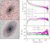 |
Fig. 2. Showcasing examples of radial profiles, as described in Sect. 3.2, using NGC 720. Top left panel: the 3.6 μm image, with masks shown via the red contours. Bottom left panel: the same image, with 2″ radial bin width, variable PA and ϵ isophotal ellipses overlaid in black. The blue ellipse shows B-band R25 from HyperLEDA, while the two red ellipses show our values of R25.5, 3.6 and R26.5, 3.6 (solid and dashed, respectively). Rightmost panels: radial profiles of, from top to bottom: surface brightness, ellipticity, and position angle. The 3.6 μm and 4.5 μm profiles are offset from each other by the amounts shown in the legends to avoid significant overlap. Profiles shown here are truncated in radius compared to those available online, to avoid clutter from poor-quality fits in the far outskirts. Vertical dotted red lines show R25.5, 3.6. |
The last used fixed centers, fixed ϵ and PA, and radial bin widths Δr = 2″: these profiles have parameters fixed to those of the μλ = 25.5 mag arcsec−2 isophotes measured using the Δr = 6″profiles described above. With fixed isophote shapes, these profiles are most useful for measuring disk scalelengths, break radii, and for performing 1D bulge-disk decompositions. With these profiles, we measured the curves of growth, from which we derived asymptotic magnitudes (Sect. 3.3) and derivative values thereof. We note that the use of these profiles relies on the assumption that the μλ = 25.5 mag arcsec−2 isophote shapes accurately reflect those of the disk’s underlying structures, such as spiral arms; more detailed analysis may require a more careful outer isophote selection to ensure this is true.
Generating these profiles required multiple steps. First, IRAF’s ellipse task simply ignores masked pixels, biasing the curves of growth. While there are options to estimate masked flux within IRAF, because many of the sample galaxies have spiral arms, bars, and other such symmetrical structures, we opted instead to estimate masked flux through our own interpolation algorithm, demonstrated in Fig. 3. For this ETG sample only, we interpolated across masks using the galaxy’s azimuthal light profile, measured in one-pixel-wide radial bins from the center outward.
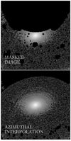 |
Fig. 3. Demonstrating interpolation across masks for a heavily masked galaxy (IC 3381). Top panel: the masked image, while the bottom panel shows the same image but with the galaxy’s light interpolated azimuthally across the masked pixels (see Sect. 3.2). |
We demonstrate this using the galaxy IC 3381, which is contaminated by a bright nearby star and so has been heavily masked. First, in each radial bin we measured the mean and standard deviations within 10-degree-wide azimuthal bins. As a first pass, we linearly interpolated this azimuthal profile across the masked pixels and recorded the median standard deviation among azimuthal bins (hereafter, σrad). In order to preserve any periodicity induced by, for example, bars, we then decomposed the resulting interpolated azimuthal profiles into Fourier modes and used the first m = 20 Fourier modes to more accurately reconstruct the flux across masked pixels. We then added Gaussian noise to the interpolated values, distributed as ∼𝒩(0, σrad). We show an example of this interpolation for the same example galaxy, IC 3381, in the bottom panel of Fig. 3.
With the missing flux now preserved, we constructed radial profiles by running ellipse twice: first, using the software described by Salo et al. (2015) to select sensible starting values for semimajor axis length (SMA), PA, and ϵ, then automatically running unconstrained ellipse fits, in the three manners described above, using these starting parameters. We chose not to constrain the automated fits in order to measure profiles to as low a surface brightness level as possible, but the outskirts of these unconstrained profiles evidently showed large swings in ϵ and PA where the fits were dominated by noise. Therefore, we derived maximum radii for the fits using the point at which the values of ϵ or PA in the Δr = 6″ profiles began to show regular 3σ divergences from their mean values as measured beyond the μ3.6 = 25.5 mag arcsec−2 isophote (or, failing this, where the ellipse uncertainty in these values, beyond μ3.6 = 25.5 mag arcsec−2, first was recorded as INDEF). We chose as the maximum fitting radius 1.2 times this value, which ensures in most cases that profiles reach at least the μ3.6 = 25.5 mag arcsec−2 isophote if the image’s noise limit is below this value, even if the isophotal fits there are poor. We then refit all profiles out to these maximum radii for each galaxy, checking the robustness of each by overplotting the fitted isophotes on the 3.6 μm images of each galaxy. Where the fitting failed (evident when the isophotal shapes were constant even at small radii), we simply reran the fits with different starting SMA until they succeeded. Due to the ETG sample galaxies’ often simple morphology, we needed only rerun in this manner one or two times.
As in MM2015, we provide these fits as ASCII tables (Sect. 6). We provide the same parameters as in MM2015, including harmonic deviations from perfect ellipses and uncertainty estimates. We also include photometric profiles corrected for PSF scattering in the same manner as in MM2015, who used correction factors taken from the IRAC Instrument Handbook1. Briefly, the light from any extended source (e.g., galaxies) in IRAC is a convolution of the astrophysical light distribution and the extended IRAC PSF. This means that, in a given photometric aperture, light from the astrophysical source is both scattered out of the aperture into the PSF wings, and scattered into the aperture from astrophysical sources outside, including other regions of the same galaxy.
Given the complexity of the IRAC PSFs, modeling this effect requires using model galaxies convolved with the measured PSF for each IRAC band. From the IRAC Instrument Handbook, PSF correction factors were measured using single-Sérsic profile model ETGs with sizes ranging up to 200″. For the total flux F within an aperture, these are provided in the following form:

where  is the equivalent elliptical aperture radius in arcseconds, and the constants A, B, and C are equal to 0.82, 0.37, and 0.91 for 3.6 μm and 1.16, 0.433, and 0.94 for 4.5 μm. Likewise, as shown by MM2015, the correction for the surface brightness within an elliptical aperture Iobs can be made via a series expansion of Eq. (1):

These correction factors are nominally accurate to within ∼10%; however, they may also contain systematic errors given the limited kinds of models used to derive them. We therefore now also include a second correction for each galaxy in our tables. Using the GALFIT Sérsic fit parameters from the fortcoming P4 analysis, we constructed both the theoretical non-convolved and the PSF-convolved 2D model images, MODEL and PSF ⊗ MODEL, respectively. We made the convolution with the same symmetrized PSF that Comerón et al. (2018) used, obtained from the data in Hora et al. (2012). To make sure the PSF has sufficient coverage, we continued the PSF tails so that the final coverage was 450″ × 450″. We then performed IRAF ellipse fits to both the non-convolved and convolved model images, using the same ellipticity and PA as for the observed profile. We denote these profiles as Inon − convolved and Iconvolved, giving an estimate

Here f is the infinite aperture correction used to correct flux of extended sources (f = 0.944 for 3.6 μm and 0.937 for 4.5 μm; Reach et al. 2005). The correction for the total flux F has the same form.
We note that in this analysis we ignored the small difference in the orientation parameters used in P4 (Salo et al. 2015) compared to our current ones: they were also estimated from IRAF ellipse profiles, but, instead of using a fixed isophotal level, correspond to the visually selected outer isophote.
Figure 4 shows example profiles using each kind of aperture correction, for comparison. We note here that, for consistency across the full S4G+ETG sample, we derived all P3 values using the aperture correction from MM2015; however, because it is tailored to specific galaxies, we recommend any future analyses using these profiles are done with the revised corrections. The choice has no noticeable impacts on the results presented in this paper; it primarily results in very slight deviations in our derived magnitudes, well below the photometric uncertainty. It does not impact any of our broader scientific conclusions. We make these new corrections available along with our data release.
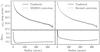 |
Fig. 4. Comparing aperture corrections for a single radial surface brightness profile. Left panels: the effect of the aperture correction described by MM2015. The black line shows the unaltered surface brightness profile for NGC 720, while the gray line shows the same profile after the aperture correction is applied. Bottom left panel: the difference between the two (unaltered−corrected). Right panels are the same as the left panels but show our more robust aperture correction using GALFIT models (see Sect. 3.2). We derived all magnitudes and related quantities using the MM2015 correction, to maintain consistency with that study; however, for any future analysis using our data sets, we recommend instead using the revised correction. |
Finally, we corrected all magnitudes and surface brightnesses for Galactic extinction using the extinction tables from Schlafly & Finkbeiner (2011). These corrections are typically extremely small (< 0.01 mag), but we include them in the interest of accuracy.
3.3. Asymptotic magnitudes
To derive asymptotic magnitudes, we followed MM2015, using each galaxy’s curve of growth (hereafter, c.o.g.). We derived a given galaxy’s c.o.g. as the cumulative sum of the galaxy’s flux within elliptical apertures of constant ϵ and PA, grown in semimajor axis in steps of 2″ and corrected for PSF effects using Eq. (1). Given the depth of the S4G+ETG, for most galaxies in our sample the relationship between the local gradient and the magnitude enclosed within each elliptical aperture becomes roughly linear near the outskirts of the c.o.g. We therefore fit a line between the local gradient and the magnitude in this linear regime; the y-intercept of this line is, by definition, the asymptotic magnitude.
Figure 5 shows examples of the c.o.g (top panels) and linear fits (inset panels) for two galaxies with different radial extents and luminosities. Particularly for galaxies with small angular sizes (hence few points in their surface brightness profiles) and low luminosities (low S/N at all radii), it is not always clear whether we are indeed reaching the flat part of the c.o.g. Additionally, because many galaxies in our sample are ellipticals with steep luminosity profiles (Sérsic n > 2), the slopes become approximately linear only at very large radii. For each galaxy, we therefore hand-picked the limits within which to fit these lines.
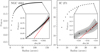 |
Fig. 5. Example curves of growth for two galaxies, one bright with a large angular size (NGC 4564, left), the other faint with a small angular size (IC 271, right). Black points in the main panels show the total magnitudes enclosed within each radius (bin width 2″). The inset panels show the local gradients in the outskirts of the curves of growth. Red dashed lines show fits to the linear parts of these gradients chosen by eye; the y-intercepts of these red lines are the asymptotic magnitudes. Gray shaded regions show the 1σ (dark gray) and 2σ (light gray) perturbations to the curves of growth from adjusting the sky subtraction (see Sect. 3.3). |
This contributes some uncertainty into the final derived magnitudes, but this uncertainty is quite small compared to the systematic uncertainty induced by the sky subtraction. Because the c.o.g. relies on summing flux in concentric apertures, a slight under- (over-)subtraction of the sky will result in a positive (negative) gradient in the outermost areas of the galaxy disk, where the sky level becomes comparable to the galaxy disk brightness, thus potentially altering the y-intercept used to derive the magnitude. To derive the uncertainties associated with the sky subtraction, we subtracted from each c.o.g. 1000 different sky levels randomly sampled from a normal distribution ∼𝒩(SKY, DSKY) (see Sect. 3.1). We took the 1σ amplitude of the variation in the final derived asymptotic magnitudes as this sky uncertainty, using our initial hand-picked fitting limits to derive y-intercepts for every perturbation. The gray shaded regions in the subpanels of Fig. 5 show the effects of these perturbations, with the dark and light gray regions showing the 1σ and 2σ variations on the c.o.g., respectively. We provide these systematic uncertainties in addition to the photometric uncertainties.
To measure absolute magnitudes, we derived distances (again following MM2015) by either taking the average of all redshift-independent distance estimates for each galaxy from the NASA Extragalactic Database (NED)2, if available (60.4% of the new sample), or by taking the average of all redshift distances available from HyperLEDA (Paturel et al. 2003).
We derived stellar masses using these distances and asymptotic magnitudes following the dust-corrected (Meidt et al. 2012) expression given by Eq. (8) of Querejeta et al. (2015):

where ℳ* is in solar masses, Fλ are the total fluxes in Jy, and D is the distance to the galaxy in Mpc. This expression was derived using the independent component analysis technique demonstrated by Meidt et al. (2012). This differs from MM2015, who used the value ℳ*/L3.6 = 0.56 from Eskew et al. (2012). We found the impact of this choice to be almost unnoticeable. One might expect some noticeable differences given that Querejeta et al. (2015) had few ETGs available for their calibration, but ETGs are also relatively dust-poor compared to LTGs (e.g., Skibba et al. 2011), and hence any dust corrections should be, and seemingly are, slight.
In the following cases, the target galaxy overlaps strongly in projection with another, much brighter object: ESO 400-30, NGC 3636, NGC 4269, NGC 5846A, and PGC 93119. The c.o.g. method is incapable of correctly measuring asymptotic magnitudes for such galaxies, as their flux cannot be disentangled from that of their brighter neighbors. We will therefore obtain more accurate magnitudes for these galaxies at a future date through 2D decompositions (Pipeline 4), taking into account both the galaxy and its neighbor simultaneously. For now, we urge caution regarding the magnitudes we provide for these particular galaxies.
3.4. Concentration indices
The radial distribution of light–the light concentration–is easily measurable and, when used in conjunction with galaxy asymmetry and clumpiness (Conselice 2003), can serve as a quantitative alternative to visual morphological class (e.g., Hubble 1926; Morgan & Mayall 1957; Morgan 1958; Okamura et al. 1984; Kent 1985; Abraham et al. 1994; Bershady et al. 2000; Conselice 2003, 2006; Taylor-Mager et al. 2007; Holwerda et al. 2014). In elliptical galaxies, the light concentration – being explicitly related to the Sérsic index n (e.g., Bershady et al. 2000; Trujillo et al. 2001) – correlates with galaxy luminosity (e.g., Caon et al. 1993; Conselice 2003; Ferrarese et al. 2006; Mahajan et al. 2015; Graham 2019 and thereby with stellar mass, suggesting that the light profile is somehow indicative of an elliptical galaxy’s evolutionary history. It is thus a rather useful first measure of a given galaxy’s intrinsic properties.
Again following MM2015, we measured the following two concentration parameters: C31 (de Vaucouleurs et al. 1977) and C82 (Kent 1985), defined as:
where Rx is the radius containing x% of the total luminosity of the galaxy (see also Fraser 1972). As in MM2015 and Bershady et al. (2000), to avoid assumptions about the shapes of the light profiles, we measured Rx from the c.o.g. Also, in constrast with, for example, Bershady et al. (2000), we extrapolated the galaxies’ total luminosities out to infinity rather than measuring them within set apertures.
3.5. Galaxy sizes
ETG mass-size relations are of considerable interest, particularly given their connection to ETG formation and evolution mechanisms (e.g., Daddi et al. 2005; Trujillo et al. 2007; van Dokkum et al. 2008; van der Wel et al. 2014). Recently, the mass-size relation for galaxies generally has come under additional scrutiny due to the recent rediscovery of sometimes abundant populations of extremely extended but low-mass galaxies in clusters, originally identified by Binggeli et al. (1985) in the Virgo Cluster, now broadly referred to as ultra-diffuse galaxies (e.g., van Dokkum et al. 2015; Koda et al. 2015; Mihos et al. 2015; Iodice et al. 2020). Depending on the size metric used, such galaxies either appear as extreme outliers in the mass-size relation or show little difference from other dwarf galaxies (Chamba et al. 2020), leading to the argument that a more physically motivated definition of galaxy size (e.g., based on star formation thresholds) is called for (Trujillo et al. 2020, and references therein).
For our ETGs, we provide 3.6 μm and 4.5 μm half-light (or effective) radii, as well as two isophotal radii: R25.5 and R26.5, denoting the radii at which the galaxy’s surface brightness profiles reach 25.5 and 26.5 AB mag arcsec−2, respectively. As NIR imaging is such a close tracer of stellar mass, the effective radius is nearly equivalent to the half-mass radius, while R25.5, 3.6 and R26.5, 3.6 denote the ∼ 3.6 ℳ⊙ pc−2 and ∼ 1.5 ℳ⊙ pc−2 surface mass density contours, respectively (using the ℳ/L calibration from Eskew et al. 2012). We measure all radii along the galaxies’ major axes; hence, all radii are deprojected. We also derive isophotal radii both from the raw and inclination-corrected surface brightness profiles.
We measured the half-light radii in the same manner as the concentration parameters described above, taking them as the radii at which the c.o.g. reaches 50% of the galaxies’ total flux (converted from the asymptotic magnitudes). We measured the isophotal radii directly from the Δr = 6″ surface brightness profiles described in Sect. 3.2 (i.e., using elliptical apertures), to take advantage of the improved S/N. Given these profiles’ rather coarse sampling, we interpolated the exact radii between the two bins that enclose the desired isophote. We recorded as well the full isophotal parameters at each radius (PA and ϵ), interpolated in the same manner. If the background noise precluded our ability to find either a 25.5 or 26.5 mag arcsec−2 isophote for a given galaxy, we recorded these values as −999 (for 3.6 μm, 20 cases and 177 cases, respectively; for 4.5 μm, 178 and 204 cases, respectively). For the remainder of this paper we focus on the μ3.6 = 25.5 isophotal radii, given their higher S/N.
All of these values – magnitudes, concentrations, sizes, and associated uncertainties (including SKY, DSKY, and RMS) – will be made available in table form on the NASA/IPAC Infrared Science Archive (IRSA), as well as at the CDS. We now showcase them, starting with a summary of observed parameters across the S4G+ETG population, then moving to a variety of NIR scaling relations.
4. Overview: General trends
The top panels in Fig. 6 show the distributions of stellar mass (luminosity), concentration, and size for the entire S4G+ETG sample, with ETGs (T ≤ 0 and T = 11; filled histograms) also displayed separately from the whole sample (unfilled histograms). The bottom panels show individual galaxies’ parameter values as a function of morphological T-type. ETGs are plotted as black points, with the full population plotted underneath in gray. Red solid lines show the median trends, with red dashed lines showing the first and third quartiles.
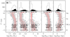 |
Fig. 6. Distributions of the photometric parameters discussed in Sect. 3 (top), and parameter values plotted against morphological T-type (bottom). From left to right: the parameters shown are: decimal logarithm of stellar mass (in solar units); concentration parameter C82 (Eq. (6)); concentration parameter C31 (Eq. (5)); logarithm of the μ3.6, AB = 25.5 mag arcsec−2 isophotal radius in kiloparsecs; and logarithm of the half-light (∼half-mass) radius in kiloparsecs. Solid red lines show the median value of each parameter measured in bins of ΔT = 1, while dashed red lines show the associated first and third quartiles. Unfilled histograms and gray points show distributions for all the galaxies, while filled histograms and black points show distributions for galaxies with T ≤ 0 and T = 11 (ETGs). |
We use T-types from Buta et al. (2015) for the original S4G sample, and new classifications by R. Buta for the ETG extension galaxies. These classifications follow the Comprehensive de Vaucouleurs revised Hubble-Sandage (CVRHS; Buta et al. 2007) system, which follows the de Vaucouleurs revised Hubble-Sandage system (de Vaucouleurs 1959) but is modified to include many additional morphological features. For quick reference, we reproduce the integer T-types associated with each broad morphological classification from Buta et al. (2015) in Table 1. A sample of the full classification table can be found in Table A.1.
Numerical T-types summary.
We focus here on the ETG population, in its context within the general population of nearby galaxies. We replicate a few previous observations. For example, the high-mass end of the galaxy stellar mass function tends to be dominated by ETGs at low redshift (e.g., Baldry et al. 2004; Pozzetti et al. 2010; Calvi et al. 2012), and in our sample the bootstrap median mass (measured as the median of the medians of 10 000 randomly resampled mass distributions, with replacement) of ETGs is indeed higher than that of either LTGs or the total galaxy population (ETGs and LTGs combined): log (ℳ*/ℳ⊙) = 10.15 ± 0.03 for ETGs only, versus 9.63 ± 0.03 for LTGs only, and 9.78 ± 0.02 for all the galaxies, where uncertainties are the 1σ bootstrap uncertainty (measured as the standard deviation of the bootstrapped median values described above) on the median (we use the bootstrap medians and uncertainties in all following comparisons). Bright ETGs also have the highest concentration (C82 = 4.40 ± 0.04 vs. 3.12 ± 0.02 for the whole sample, and C31 = 5.13 ± 0.09 vs. 3.13 ± 0.02). Nearby ETGs are also larger in isophotal size compared to either LTGs or the whole galaxy population (median R25.5 = 12.74 ± 0.36 kpc, vs. R25.5 = 9.91 ± 0.16 kpc for LTGs, and R25.5 = 10.47 ± 0.15 kpc for all the galaxies); combined with the previous point, this results in them having smaller effective radii on average (median Reff = 2.30 ± 0.11 kpc vs. Reff = 4.47 ± 0.08 kpc for all the galaxies; a similar trend was also noted by Jarrett et al. 2003).
More granular trends are also visible. S0s (−3 ≤ T ≤ 0) are undermassive compared to early-type spirals (Sa, Sab, Sb), with median log (ℳ*/ℳ⊙) = 10.23 ± 0.03 compared to log (ℳ*/ℳ⊙) = 10.39 ± 0.01. S0s are closer in mass to Sc galaxies (log (ℳ*/ℳ⊙) = 10.10 ± 0.01). This too was shown previously, by van den Bergh (1998). Most of this low-mass tendency is driven by early-type S0s (S0− and S00), which have median mass log (ℳ*/ℳ⊙) = 10.09 ± 0.05, compared to log (ℳ*/ℳ⊙) = 10.36 ± 0.01 for S0+ and S0a galaxies, making Sc and early-type S0s the most similar in mass. S0s are also smaller on average in isophotal radius (R25.5 = 12.65 ± 0.38 kpc) than all but Sc (R25.5 = 12.62 ± 0.35 kpc) and dwarf galaxies (T ≥ 8, with median R25.5 = 6.49 ± 0.16 kpc), although S0s are more concentrated (hence have smaller Reff) than such dwarf disks. Again, this tendency toward small size among S0s is driven by the early-type S0s (R25.5 = 11.30 ± 0.72 kpc, compared to R25.5 = 13.36 ± 0.63 kpc for late-type S0s).
Many ETGs classified as T = 11, which are morphologically dwarf galaxies, have masses of log (ℳ*/ℳ⊙) > 10.0, suggesting that they are not best classified as dwarfs in terms of their masses. The reason for this is unclear; either their morphological classifications do not match their high stellar masses or the distances we used to derive their masses are incorrect. The median distance to these T = 11 galaxies is 17.6 Mpc; at this distance, a dwarf galaxy with a diameter D25 < 1 kpc would have a angular size of < 12″ and hence should have been excluded from the sample via the criterion of D25 > 1′ (Sect. 2), which biases the sample against dwarf galaxies even within the selected distance constraints (D ≲ 40 Mpc). However, because these T = 11 galaxies tend to follow the rest of the ETGs in each scaling relation we examine, we will defer a detailed discussion of them for future work.
On average, LTGs and ETGs show clear disparities in concentration, as noted already by de Vaucouleurs (1948). Specifically, this disparity sets in for galaxies with T ≤ 3 (Sb), with both concentration parameters rising monotonically with decreasing T below this value (this trend is visible already with the smaller ETG sample from Muñoz-Mateos et al. 2015, e.g., their Fig. 9) save for a slight dip among early-type S0s (−3 ≤ T ≤ −2). Díaz-García et al. (2016) found similar morphological separation using stacked profiles, which was echoed in the central stellar contribution to the circular velocity curves. This likely reflects the similar steady increase in the bulge-to-total luminosity ratio (B/T) with decreasing morphological type observed by, for example, Laurikainen et al. (2010).
5. Scaling relations
Here we showcase several ETG scaling relations derived from the P3 isophotal parameters. We begin with concentration, then move to size, surface brightness, and finally discuss integrated m3.6 − m4.5 colors. At the end of each subsection, we briefly summarize our results.
5.1. Concentration
Particularly for high-redshift galaxies, where individual morphological features are unresolvable, light concentration is useful for separating ETGs and LTGs (e.g., Morgan 1958; de Vaucouleurs & Agüero 1973; Okamura et al. 1984; Kent 1985; Conselice 2003). Concentration also scales with luminosity, showing an almost log-linear relationship for ETGs (e.g., Schombert 1986; Binggeli & Cameron 1991; Graham et al. 2001; Conselice 2003; Kauffmann et al. 2004), which we demonstrate as well in Fig. 7. Structural parameters such as concentration in turn show little dependence on local environment, but environment correlates well with star formation rate (e.g., Kauffmann et al. 2004; van der Wel 2008), suggesting that the structure of the bright, visible parts of galaxies was in place early on in most galaxies (Kauffmann et al. 2004). Still, secular evolution and subsequent star formation episodes can modify galaxy structure over time, so even under this early formation scenario one might expect that galaxies with bars, spiral arms, and other dynamical structures capable of moving mass (e.g., Sellwood & Binney 2002), as well as those with ongoing, widespread star formation, might show the largest scatter in the concentration – stellar mass relation. Indeed, Méndez-Abreu et al. (2021) found that disk galaxy bulges evolve little over cosmic time, while their disks can change dramatically (depending on the central concentration of the galaxy, e.g., Athanassoula et al. 2005). Additionally, Sheth et al. (2008) showed that the distribution of bars among massive S0s at z = 0.84 was quite similar to that of massive S0s at z = 0, suggesting that the disk structures were in place early on in these galaxies; lower-mass LTGs, by contrast, appear to have formed their bars much more gradually during this time, but evidently continued forming stars in their disks much longer than their S0 counterparts. We see evidence for this in Fig. 7. Ellipticals (navy blue points) show a fairly tight correlation; S0s (yellow and gold points) of the same stellar mass scatter toward low C82 values, with the tightest scatter found at the high-mass end; and the scatter and distribution of C82 values among LTGs is quite similar to that of S0s, with the highest scatter at the lowest stellar masses.
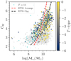 |
Fig. 7. Correlation between concentration and stellar mass. Here and in all subsequent figures with this color scheme, we show ETGs (T ≤ 0) color-coded by T-type, while we show all S4G galaxies in gray. We show dwarf ETGs (T = 11) in cyan. The dashed black line shows a linear fit between log (ℳ*/ℳ⊙) and log (n), converted from C82, for ETGs (Eq. (7)). The red dashed line shows a similar fit, but here n was estimated for each ETG via single-component 2D decompositions (Eq. (8)). |
Though this correlation appears roughly log-linear, it does show some mild curvature, suggesting the true log-linear correlation is between stellar mass and Sérsic index (e.g., Caon et al. 1993; Young & Currie 1994; Graham 2001, 2019; Ferrarese et al. 2006; Savorgnan et al. 2013). We demonstrate this via the black dashed curve in Fig. 7, which we derived by first converting our measured values of C82 for ETGs (colored points) to their corresponding values of n (see, e.g., Graham & Driver 2005; Janz et al. 2014), then fitting the resulting log (ℳ*/ℳ⊙)–n relationship as a line:

We then converted this linear fit back to a relation between log (ℳ*/ℳ⊙) and C82 using the relation between n and C82, which produces the aforementioned black dashed curve. Using the single-component decompositions described in Sect. 2, we also derived empirical values of n for all ETGs for comparison. These too showed a linear relationship with stellar mass, which we overplot in Fig. 7 via the red dashed line (again, converted to C82). This has the form

which has a similar zeropoint but a slope different by nearly a factor of ∼1.5. Even though we are using the PSF-corrected radial profiles to derive C82, the values of n implied by our concentration parameters thus agree poorly with those derived via single-component 2D fits.
We expand on this in the top-left panel of Fig. 8, which shows our C82 values plotted against the values of n for all our ETGs derived from single-component GALFIT decompositions. The solid black line here shows the theoretical relationship between C82 and n, while the dashed line (here and in all subsequent panels) shows the median trend for all the galaxies (again shown in gray) as measured within consecutive equal-width C82 bins. Clearly, at the high-concentration (high-mass) end, the measured values of C82 are too low compared to the theoretical expectation from the measured n.
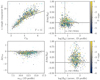 |
Fig. 8. Investigating the divergence between the Sérsic n derived from C82 and that measured from single-component 2D decompositions. Top-left panel: concentration parameter vs. Sérsic index, the latter being derived from single-component 2D decompositions for all S4G galaxies. The solid black line shows the theoretical behavior of C82 for Sérsic profiles of varying n. Here and in subsequent panels, the dashed black line shows the median of points in equal-width bins (bins with fewer than five points are ignored). Bottom-left panel: we show the difference between our asymptotic magnitudes and those derived from decompositions (negative numbers mean the asymptotic magnitudes are fainter). The solid black line here and in the following panels shows a value of 0 (no difference). Top-right panel: difference between R20 derived from single-component decompositions and those derived from our curves of growth for 3.6 μm imaging. The vertical dotted line shows the size of three IRAC 3.6 μm resolution elements. Bottom-right panel: the same as the top-right panel, but shows the behavior of R80. ETG data points are multicolored (with dwarfs in cyan), while LTGs are shown in gray. |
Venhola et al. (2018) found superficially similar behavior for galaxies in the Fornax Cluster region using Fornax Deep Survey (Peletier et al. 2020) u′-, g′-, r′-, and i′-band imaging (see their Fig. 13). Like us, Venhola et al. (2018) observed that the Sérsic n values from single-component GALFIT decompositions were systematically higher than the theoretical values of n estimated from C82. In their case, the aperture magnitudes and the corresponding C82 values were calculated using a region within one Petrosian radius, which was also taken into account in their theoretical n versus C82 relation (the n corresponding to a given C82 is larger than if infinite extent is assumed). They concluded that the offset, seen for all values of n, was due to resolution effects: the GALFIT decompositions included PSF-convolution, whereas the aperture photometry did not3.
We investigate this explicitly in the right two panels of Fig. 8. In these two panels, we show the values Δlog (Rx) = log (Rx, 1 comp.)−log (Rx, c.o.g.), where x is the fraction of light contained within the radius, “1 comp.” represents values derived from single-component decompositions, and “c.o.g.” represents values we derive from the radial curves of growth. We show both components used for C82, the 20% (top-right panel) and 80% (bottom-right panel) flux radii. Vertical dotted lines in each panel show three times the 3.6 μm FWHM; if resolution was purely at fault for the diverging C82–n profiles, because R20 often falls within this limit, it might show the strongest method-to-method difference. However, while Δlog (R20) is systematically slightly positive (albeit with large scatter), the offset is small compared to that of Δlog (R80), for which resolution’s impact should be mild. Resolution does not thus appear to be the driving factor here.
Typically, we find Δlog (R80) > 0, indicating that single-component-fit R80 are systematically ∼1.3 times larger on average (albeit with large scatter) than those derived from the curves of growth. In the bottom-left panel of Fig. 8, we also show the difference between the magnitudes estimated from single-component Sérsic fits and our asymptotic magnitudes. These tend to be negative, meaning single-component fit magnitudes are systematically ∼0.2 mag brighter than asymptotic magnitudes. This, combined with the larger values of R80, suggests that single-component fitting often overestimates the flux in the galaxies’ outskirts. This is expected for disk galaxies, which often show down-bending breaks in their surface brightness profiles (e.g., Pohlen & Trujillo 2006; Erwin et al. 2008). However, from the color distribution of the points, it is clear that the magnitude of the difference is similar for all ETG morphological types. Various studies have shown that elliptical galaxies, much like disks, are poorly characterized by single Sérsic component models (e.g., Schombert 1986; Hopkins et al. 2009), which may result in the behavior we see here.
We provide further evidence for this in Fig. 9. In each panel, we show the difference between decomposition magnitudes – both single- and multicomponent – and asymptotic, c.o.g-derived magnitudes, as a function of C82, for the original S4G sample. Asymptotic magnitudes and C82 here come from MM2015, while multicomponent decomposition magnitudes come from Salo et al. (2015). Both decomposition magnitudes show slight systematic offsets from the asymptotic magnitudes, as well as trends with C82: the higher the concentration, the brighter the estimated decomposition magnitude relative to the asymptotic value. However, this trend is much stronger for the single-component decompositions than for the multicomponent decompositions. Additionally, ∼0.06 magnitudes of the offset in the multicomponent magnitudes arises because these magnitudes were derived directly from the images, without applying the 3.6 μm infinite aperture correction of 0.944 (see Eq. (3), and Reach et al. 2005). This confirms our suspicion that single-component fits are not as reliable as either multicomponent fits or the c.o.g. method for estimating total galaxy magnitudes. Combined with Fig. 8, it is clear that most of the systematic errors in single-component fits occur in the galaxy outskirts.
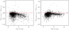 |
Fig. 9. Comparing single- and multicomponent decomposition magnitudes with c.o.g. magnitudes. Left panel: difference between single-component decomposition total magnitudes and asymptotic magnitudes (P3; MM2015), as a function of c.o.g. concentration parameters (P3) for the original S4G sample. Right panel: as the left panel, but showing the difference between multicomponent decomposition total magnitudes (P4; Salo et al. 2015) and asymptotic magnitudes. While both decomposition types show slight offsets from the asymptotic magnitudes on average, as well as downward trends (brighter magnitudes) with increasing concentration, the downward trend in the single-component decompositions is much stronger than that in the multicomponent decompositions. Also, at least ∼0.06 magnitudes of offset in the multicomponent magnitudes arise because we applied no infinite aperture correction to the total flux (see Eq. (3), and Reach et al. 2005). |
In summary, we reproduce well the known trend between C82 and stellar mass for ETGs, thereby reproducing the trend between n and stellar mass (Fig. 7). In comparing our values of C82 derived from radial profiles to those derived from single-component GALFIT decompositions, we find that such decompositions tend to overestimate the concentration and the total flux of these galaxies (Fig. 8). Most of this over-estimate of flux occurs in the galaxy outskirts, in a manner that correlates with the galaxies’ concentration. Multicomponent decompositions fare much better–total magnitude estimates from these agree more closely with radial profile–derived asymptotic magnitudes, with only small systematic differences due to galaxy concentration (Fig. 9).
5.2. Mass-size
The mass-size relation for ETGs has been crucial to understanding the growth of ETGs throughout cosmic history (e.g., Daddi et al. 2005; Longhetti et al. 2007; Toft et al. 2007; Trujillo et al. 2007; Hopkins et al. 2008; van Dokkum et al. 2008; Hopkins et al. 2009; van der Wel et al. 2009; Szomoru et al. 2012; Andreon et al. 2016). A series of gas-poor, low mass-ratio mergers can explain elliptical galaxies’ rapid growth in size compared to stellar mass (e.g., Nipoti et al. 2003; Naab et al. 2009; Szomoru et al. 2012), though dissipational processes seem necessary to explain specific aspects of their evolution (e.g., the tilt in the fundamental plane Hopkins et al. 2008). Typically, size is measured via the effective radius, given the utility of Sérsic functions in describing their light profiles (though see Sect. 5.1), but it has long been known that all galaxies also show correlations between isophotal size and absolute magnitude (or, modulo the mass-to-light ratio, stellar mass; Schombert 1986; Binggeli & Cameron 1991). These correlations are always positive, suggesting that whatever drives the mass evolution of most galaxies drives the size evolution in a similar way.
MM2015 showed the stellar mass-Reff relation for the initial 2352-galaxy S4G sample (their Fig. 15). They demonstrated a clear morphological segregation, with ETGs occupying the lower-right (low-luminosity, compact) corner of the point distribution and the latest type galaxies (Sm, Irr) occupying the lower-left (low-luminosity, extended). We broadly reproduce this trend in Fig. 10. Gray points here are LTGs, while ETGs are color-coded by morphological type. Among ETGs, ellipticals and S0s are mostly intermingled, though for stellar masses ≳ 1010 ℳ⊙, S0s show a mild tendency toward higher Reff than ellipticals at equal stellar mass. ETGs as a population form a visibly tighter stellar mass-Reff relation than LTGs, even including the increase in dispersion emerging below stellar masses ≲ 1010.5 ℳ⊙.
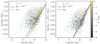 |
Fig. 10. Effective radius mass-size relation. Left panel: our effective radius values (derived from 3.6 μm imaging) plotted against stellar mass, with a linear fit to ETGs with masses > 1010.7 ℳ⊙ shown in black and the z = 0.25 ETG mass-size relation from Newman et al. (2012) shown in green (labeled N12). Right panel: the same as the left, but here Reff has been adjusted by a factor of |

Only the high-mass end of the relation is roughly linear: curvature in the mass-Reff relation is known to result from the dependence of light profile shapes on stellar mass (Sect. 5.1), alongside structural differences between dwarf and massive ETGs (e.g., Graham & Guzmán 2003; Boselli et al. 2008; Janz & Lisker 2008; Kormendy et al. 2009). Massive galaxies are also not well-described by single Sérsic profiles (Figs. 8 and 9), likely leading to divergences even from the theoretical curved relationship described by Graham & Guzmán (2003) and others. For comparison with past studies, however, in Fig. 10 we show a linear fit to the S4G mass-size relation via the black lines, including only those ETGs with stellar masses > 1010.7 ℳ⊙ (126 galaxies total). This has the following form:

We overplot similar fits from two previous studies of nearby galaxies, derived above similar stellar mass thresholds: in the left panel, we show the fit for z = 0.06 ETGs from Table 1 of Newman et al. (2012); and in the right panel, we show the ETG sample fit from Eq. (17) of Shen et al. (2003). These have the following forms:

for the Newman et al. (2012) relation (labeled N12 in Fig. 10), and

for the Shen et al. (2003) relation (labeled S03 in Fig. 10). We have corrected our rightmost panel effective radii by a factor of  (with axial ratios measured at R25.5, 3.6) for this comparison, as Shen et al. (2003) used circular apertures for their photometry (see MM2015).
Our fit is very close to those of both Newman et al. (2012) and Shen et al. (2003). Our derived slope is slightly shallower than those of either study, and our intercept is very close to that of Shen et al. (2003) but noticeably smaller than that of Newman et al. (2012). While this may have physical significance – for example, the change in intercept compared with that of Newman et al. (2012) could imply a size evolution since z = 0.06 – we note that both Newman et al. (2012) and Shen et al. (2003) used Sérsic fits (via GALFIT and from the radial profiles, respectively) to derive their masses and radii, so the differences could also be explained by differences in methodology (see Sect. 5.1). For example, van der Wel et al. (2014) found a substantially different slope of 0.75, which they attribute to differences in sample selection and their use of Petrosian (Petrosian 1976) half-light radii. Additionally, the aforementioned studies used visible light photometry to estimate stellar mass for their z = 0 samples, which can be more subject to, for example, metallicity effects (e.g., Meidt et al. 2014). Within these ambiguities, therefore, we find our fits broadly consistent with those of previous studies, confirming the z = 0 calibration for the observed tendency for the slope in this relation to remain stable since as early as z = 3 (e.g., van der Wel et al. 2014).
We show the stellar mass-isophotal size relation for S4G+ETG galaxies in Fig. 11, using R25.5, 3.6 for the isophotal radii. This relation looks similar when using R26.5, 3.6 or the isophotal radii measured in 4.5 μm, but these have higher scatter due to lower S/N. The left panel shows the relation using unmodified surface brightness profiles, while the right panel shows the relation after correcting the surface brightness profiles to their face-on equivalents. We do this by multiplying the flux in each radial bin by the axial ratio, following Kent (1985); we note that, while such a correction may be an appropriate inclination correction for thin disks, for ETGs, many of which have spheroidal or triaxial shapes, this correction should be considered an isophotal circularization rather than a true inclination correction. The scatter decreases substantially once this correction is applied. Extreme outlier points in the rightmost panel (mostly LTGs) are all nearly edge-on galaxies with unreliable axial ratios. Outliers among the ETGs have a muddier origin; for example, the point at (log (ℳ*/ℳ⊙) = 9.657, log (R25.5, 3.6) = 1.129, shown by the arrow) is IC 3413, a seemingly undisturbed, mildly inclined, and mostly featureless galaxy, though it is a Virgo Cluster member. Deeper imaging of some of these outliers could reveal evidence of tidal interactions, which may move them away from their expected positions in this relation.
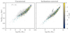 |
Fig. 11. Isophotal mass-size relation. Left panel: the relation between R25.5, 3.6 and stellar mass, in which R25.5, 3.6 was derived from the raw surface brightness profiles. Right panel: the same but with R25.5, 3.6 corrected for inclination, measured from the outermost isophote shapes’ axial ratios. ETG data points are multicolored (with dwarfs in cyan), while LTGs are shown in gray. The arrow indicates the galaxy IC 3413 (see text). |
MM2015 show the stellar mass-size relation for the initial S4G sample in their Fig. 14, again demonstrating clear morphological segregation, which accounts for much of the scatter in the left panel of Fig. 11. Once an inclination correction is applied4, this morphological segregation reduces, as the wider array of axial ratios displayed by thin disk galaxies results in stronger corrections on average compared to the vertically thicker ellipticals. Yet, with only an axial ratio correction applied, the scatter reduces just as much for elliptical galaxies as for S0s, surprising given that ellipticals are usually oblate systems. Possibly this correction is as effective for elliptical galaxies due to their significant rotational support (e.g., Cappellari et al. 2007), which implies that their axial ratios are in some ways reflective of their instrinsic alignments. We show this explicitly in Fig. 12, in which we plot the axial ratios of galaxies overlapping the S4G+ETG and the ATLAS3D (Cappellari et al. 2011a; Emsellem et al. 2011) surveys against their rotational velocity–to–velocity dispersion ratios (V/σe, measured at one effective radius; Emsellem et al. 2011). Even with the ambiguity presented by nearly edge-on galaxies (marked with red circles), there is a clear downward trend, as expected if more rotationally supported galaxies are also intrinsically vertically thinner. We show ellipticals as orange points and S0s as black points – the downward trend is visible using both classes of galaxies.
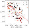 |
Fig. 12. Comparing V/σe values (denoting those measured at 1 Reff) from the ATLAS3D survey to isophotal axial ratios measured at R25.5 for galaxies matching between the S4G+ETG and ATLAS3D samples. Orange points denote elliptical galaxies, while black points denote S0s. The red dashed line shows a linear fit to all points. Points circled in red are edge-on disks (denoted “spindle” by Buta et al. 2015), with unreliable axial ratios. |
The tightness in the stellar mass-isophotal radius relation is noteworthy, and has been mentioned before in studies utilizing different isophotes and photometric bands (e.g., Schombert 1986; Binggeli & Cameron 1991; Saintonge & Spekkens 2011; Hall et al. 2012). Indeed, several papers have recently begun to explore it in the context of star formation thresholds, assessing the shape and scatter of the relation for the radius at which the stellar mass surface density reaches 1 ℳ⊙ pc−2 (Chamba et al. 2020; Trujillo et al. 2020; Sánchez Almeida 2020), which is comparable to previous estimates of star-formation thresholds using gas surface density (3–10 ℳ⊙ pc−2, e.g., Schaye 2004). The scatter in the right panel of Fig. 11 is roughly equivalent to that found by Trujillo et al. (2020), who used g- and r-band imaging from the IAC Stripe82 Legacy Project (Fliri & Trujillo 2016; Román & Trujillo 2018) to derive stellar masses. Comparing to their Fig. 4, the curvature we find in our relation is even quite similar, as is the morphological segregation. This is not particularly surprising, as 3.6 μm imaging is a very close tracer of stellar mass – the 1 ℳ⊙ pc−2 radius explored by these papers corresponds roughly to R27, 3.6. Sánchez Almeida (2020) demonstrated that the likely origin of this low scatter lies in the anticorrelation between Reff and n, and found that it minimizes when using the 2.4 ℳ⊙ pc−2 mass surface density radius (very close to our R25.5, 3.6 ∼ 3.5ℳ⊙ pc−2). Still, the physical origin behind such an optimal value is unknown. More careful analysis of this relation is required (akin to that done by, e.g., Ouellette et al. 2017), which will be the subject of a separate paper.
In summary, we find good agreement with previous studies in the stellar-mass-Reff relation for high-mass ETGs, modulo methodological differences. We also find that the stellar-mass-isophotal radius relation, once the surface brightnesses are corrected for inclination, has very little scatter even among elliptical galaxies, which serves as a secondhand demonstration of their rotational support.
5.3. Surface brightness
While concentration parameters provide an easy-to-measure approximation of galaxy structure, surface brightness profile shapes contain much more detailed information, including the true central surface brightness, μ0. In a typical hierarchical accretion scenario, a galaxy’s core will form early, during a cosmological era in which the horizon was small and therefore mergers were more frequent, whereas the outskirts form later from less frequent mergers (Frenk et al. 1985) and from the reorganization of matter due to secular processes (e.g., Kormendy & Kennicutt 2004). This reorganization process builds the very dense innermost structures that μ0 traces (classical bulges; Sandage 1961). Subsequent secular processes can lead to mass growth in galaxy cores as well, if the bar induces angular momentum loss in the gas and dust (e.g., Athanassoula 1992; Maciejewski et al. 2002; Carles et al. 2016), but the resulting structures are often less dense and more disk-like (pseudobulges or disky bulges, in the nomenclature of Kormendy & Kennicutt 2004; Athanassoula 2005, respectively) than classical bulges. In the absence of star formation, the reorganization of mass in the disk then depends on the growth of bars, whose pattern speeds set the locations of resonances. This in turn depends on a large number of properties of the galaxy (Athanassoula 2003), including the mass and size of the central mass concentration (e.g., Sellwood 1980; Norman et al. 1996; Athanassoula et al. 2005; Debattista et al. 2006; Kataria et al. 2020), which is often small or negligible in S0s (Laurikainen et al. 2007, 2010). Elliptical galaxies lack large-scale bars and the disks necessary to form them; they also have the densest cores, which show little evolution over cosmic time (e.g., Szomoru et al. 2012), implying a two-phase evolutionary process, with early violent growth in the core followed by a slower, merger-fueled growth in the outskirts that had little impact on subsequent core evolution. In the highest-mass ellipticals, however, subsequent core evolution can occur through scouring effects of SMBH mergers and the subsequent reorganization of matter while the systems relax (e.g., Milosavljević & Merritt 2001). Modulo resolution effects (for example, the resolution of our profiles is likely too coarse to accurately probe the SMBH’s sphere of influence), surface brightness profile shapes can reflect all of these complex histories.
For an overall picture, Fig. 13 shows the radial surface brightness profiles of every ETG (T ≤ 0) in the S4G+ETG sample, with radii normalized by Reff, 3.6. We show here the fixed isophotal parameter, 2″ radial bin width curves described in Sect. 3.2. In the left panel, each curve is color-coded by the galaxy’s total stellar mass, while in the right panel the curves are color-coded by T-type. Additionally, to reduce noise in the plot, we truncate each curve at μ3.6 = 27.5.
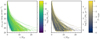 |
Fig. 13. All ETG 3.6 μm surface brightness profiles (fixed isophotal parameters, Δr = 2″; see Sect. 3.2), normalized by effective radius. Left panel: profiles color-coded by total stellar mass, while the right panel shows profiles color-coded by morphological T-type. Surface brightness is converted to mass surface density in the right panel as well, for convenience. Data quality at very low surface brightness is poor, and hence all profiles are truncated at μ3.6, AB = 27.5. |
Mass segregation is clear in the left panel, with high-mass galaxies typically showing higher surface brightnesses than low-mass galaxies at all radii. High-mass galaxies are also larger than low-mass galaxies relative to their effective radii (see also Sect. 5.2). This, combined with the tendency for high-mass ETGs to have more concentrated light profiles (Fig. 7), leads to high-mass ETGs showing longer profiles in this space. By contrast, the profiles are well-mixed by morphological T-type, suggesting that stellar mass is the primary driver behind ETG surface brightnesses. A more detailed examination of individual profiles is evidently necessary to disentangle the various contributions to the shapes of these profiles, including bars, rings, disk breaks (e.g., Pohlen & Trujillo 2006), and cored versus Sérsic ellipticals (e.g., Kormendy & Bender 1996; Faber et al. 1997).
We thus expand on the stellar-mass-surface brightness relation in Fig. 14, in which we plot only the central surface brightnesses μ0, 3.6 of each galaxy against their stellar masses. As in Fig. 8, we show μ0, 3.6 derived both from single-component 2D decompositions, as well as those derived through single-component least-squares fitting to the curves shown in Fig. 13. We correct for PSF effects in the 1D curve fits by using the aperture-corrected profiles described in Sect. 3.2.
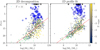 |
Fig. 14. 3.6 μm central surface brightnesses (μ0, 3.6) vs. stellar mass. Left panel: μ0, 3.6 derived from single-component 2D decompositions, while the right panel shows μ0, 3.6 derived by fitting generalized single Sérsic functions to each galaxy’s radial surface brightness profile (fixed isophotal parameter, Δr = 2″, with aperture correction applied; see Sect. 3.2). Galaxies with fitted n > 7 are circled in blue. Linear fits to the two distributions are shown via the red dashed lines, excluding galaxies with ℳ*/ℳ⊙ < 8 and fitted n > 7. Points lying above the axis limits are shown as up-pointing arrows; each of these had fitted n > 7. ETG data points are multicolored (with dwarfs in cyan), while LTGs are shown in gray. |
Either method demonstrates clear stellar mass-μ0 trends, such that higher-mass galaxies have higher central surface brightnesses, in agreement with, for example, Graham (2019, and references therein). Linear fits to these relations result in the following (excluding galaxies with ℳ*/ℳ⊙ < 8 and fitted n > 7):

for the 2D decompositions, and

for the values derived from curve-fitting. The two fits are somewhat similar despite the differing methods used to estimate μ0, 3.6, though the profile-fit slope is noticeably shallower than the decomposition slope.
In both cases, many galaxies with masses between ∼ 109.5 ℳ⊙ and ∼ 1011 ℳ⊙ lie far above the relation, meaning they have large estimated central light enhancements. Most of these have very high fitted Sérsic indices (n > 7, which we have marked using blue circles). Examination of individual profiles shows that these galaxies typically have strong central peaks indicative of large, bright bulges (relative to their disks), which thus dominate the profiles’ curvature. The distribution of these galaxies’ T-types is also heavily weighted toward disks, with the strongest peak at T = 0. Due to the complex structure of disk galaxies (which can host bulges, bars, disks, lenses, rings, nuclear bars, nuclear rings, and even active galactic nuclei), the very high fitted values of n and μ0, 3.6 we find for these galaxies may mostly result from poor fits to the galaxies’ total light profiles.
Among ellipticals, we see some hint of a light deficit for many galaxies with masses > 1010.5 ℳ⊙. The distribution of a fair number of points falls well below the fitted line in this mass regime, seemingly leveling out at a central surface brightness of ∼15 (this is clearer in the right panel of Fig. 14). These may be examples of cored ellipticals, which do tend to be high-mass galaxies (e.g., Kormendy & Bender 1996; Emsellem et al. 2007; Kormendy et al. 2009; Dullo & Graham 2012), though we note that many ellipticals in this mass range lie roughly on or above the best-fit relation as well. Whether the massive galaxies that fall on the relation are truly uncored or not is unclear given the large uncertainties inherent to our estimates of μ0, as evidenced by the many poor, n > 7 fits, described above; higher resolution profiles for the cores, in conjunction with more detailed fitting procedures, are needed to verify this.
Thus, while we broadly reproduce the known relation between stellar mass and μ0, evidently great care is required when estimating the central surface brightnesses of galaxies. As we demonstrated with the concentration index in Sect. 5.1, single-Sérsic component fits can be inaccurate and misleading.
Given this, we also investigate scaling relations using the mean surface brightnesses within fixed radii. We show two scaling relations of this nature in Fig. 15: the mean surface brightness within Reff, ⟨μ3.6, eff⟩ (left panel) and the mean surface brightness within 1 kpc radius, ⟨μ3.6, 1kpc⟩ (right panel), both plotted against stellar mass. The former relation has been demonstrated since photometry of low-mass, low-surface-brightness galaxies became possible, and was always known to have a fairly high scatter (e.g., Impey et al. 1996). A more recent demonstration of this relation came from Sedgwick et al. (2019), who found a correlation between effective r-band surface brightness and stellar mass for core-collapse supernova host galaxies with a slope of ∼ − 1.35. Our regression line is shown in Fig. 15, and has the following form:

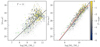 |
Fig. 15. Mean surface brightness within the effective radius (left panel) and within 1 kpc (right panel) vs. stellar mass. The solid black lines in both panels show linear fits to all S4G+ETG galaxies. The dashed red lines in the right panel show fits to only ETGs, separated at log (ℳ*/ℳ⊙) = 10.4 (see text). ETG data points are multicolored, while LTGs are shown in gray. |
where the steeper slope than that of Sedgwick et al. (2019) likely arises from the difference in photometric band and galaxy sample (core-collapse SNe hosts typically being star-forming galaxies). In NIR, ETGs and LTGs both follow similar relations, although below log (ℳ*/ℳ⊙)∼10 ETGs trend slightly higher in effective surface brightness than LTGs of the same stellar mass. This is to be expected, however, as ETGs in this mass range also have smaller Reff on average than LTGs (Fig. 10) and higher C82 (Fig. 7). Much of the scatter in this relation thus might arise from the large range of relative physical radii probed by Reff for galaxies with a variety of photometric profiles.
A more consistent choice of physical radius yields a much tighter correlation, as we demonstrate in the rightmost panel of Fig. 15 via the ⟨μ3.6, 1kpc⟩–log (ℳ*/ℳ⊙) relation. This, too, is a known feature of ETGs; Saracco et al. (2017), for example, found a tight relation between stellar mass and the mass surface density within 1 kpc ( ) among ETGs at a wide range of redshifts (see also Saracco et al. 2012; Tacchella et al. 2016; Arora et al. 2021), indicating that the average core densities of these galaxies have not evolved much during the past ∼10 Gyr (echoing, in a different manner, the results found by Szomoru et al. 2012, and references therein).
The linear fits shown by the red dashed lines mirror those done by Saracco et al. (2017), who found a kink in the  –log (ℳ*/ℳ⊙) relation at log (ℳ*/ℳ⊙)∼10.4. Here we fit only ETGs, with T ≤ 0, for better comparison with that study. Tacchella et al. (2016) found a similar bend using galaxy models from a hydrodynamical cosmological zoom simulation, although they placed its location at log (ℳ*/ℳ⊙)∼10.2. Both find a low-mass-end slope in this relation of nearly 1 and a high-mass-end slope of ∼0.6. If we split our ETG population as Saracco et al. (2017), we find the following linear fits for the low- and high-mass end, respectively:


For easier comparison, we convert our surface brightnesses to stellar mass surface densities using the relation given by Eq. (A.5) from Muñoz-Mateos et al. (2013), which yields


where  is in units of ℳ⊙/kpc2. The low-mass-end fit is very close to that found by Saracco et al. (2017), though we find a slightly shallower high-mass-end fit. Recently, Arora et al. (2021) compared this relation between many different studies, and found that all of them showed similar behavior: LTGs and low-mass ETGs show similar slopes, while high-mass ETGs show a much shallower slope. They replicate this in their own study as well, though they provide a different location for the high-mass bend than either study cited above: log (ℳ*/ℳ⊙)∼10.7.
The bend does appear to be real, and not just a result of increased scatter at the high-mass end of the relation: if we do a similar double-fit for LTGs, we find slopes in the μ3.6–log (ℳ*/ℳ⊙) relation of −2.1 and −1.9 for the low- and high-mass end, respectively, both very similar to the low-mass-end fit for the ETGs despite the higher scatter. Likewise, a fit to the entire S4G+ETG population, shown in black, has the form

which, when converted to mass surface density, has a slope of ∼0.93, very close still to the slope of ∼1.02 given by Saracco et al. (2017) for the low-mass end of their ETG relation, and very similar to the ETG+LTG best-fit slope of 0.91 found by Arora et al. (2021). Both S0s and ellipticals contribute to the bend in the relation at high stellar mass; the relation’s high-mass-end slope is −1.23 including only ellipticals, and −1.28 including only S0s.
The range of values in ⟨μ3.6, 1 kpc⟩ for ETGs above 1010.4 ℳ⊙ are the same as those for LTGs in the same mass range. The most evident morphological divide in this relation lies between ETGs and LTGs below this stellar mass, where ETGs occupy the high-surface-brightness end of the distribution at a given stellar mass, which is interesting if ETGs indeed evolve directly from LTGs. In disk galaxies, 1 kpc is well within the typical sizes of bars and possibly related structures such as rings or lenses (on average, ∼4 kpc; Laurikainen et al. 2011, 2013, and references therein), and hence this metric ⟨μ3.6, 1 kpc⟩ traces the regime of central structure, such as bulges.
If ETGs do evolve directly from LTGs, the bend at high stellar masses could imply that whatever mechanisms causing the evolution increase central densities only in lower-mass galaxies, leaving high-mass ETG cores untouched relative to their LTG ancestors. Kim et al. (2012), for example, found evidence for the immutability of high-mass ETGs by demonstrating that the cores of ETGs in their sample with clear tidal debris lie on the same Kormendy (1977) relation as their undisturbed counterparts. This could be related to bulge formation. The bulge-to-total ratio for S0s increases with increasing galaxy mass (see Fig. 7 of Laurikainen et al. 2010), and, as stated previously, large bulges tend to inhibit bar formation (Kataria et al. 2020, and references therein). This in turn could stabilize gas and dust against angular momentum loss (e.g., Athanassoula 1992; Maciejewski et al. 2002; Carles et al. 2016), or inhibit the formation of inner rings (assuming such structures are related to bar resonances; e.g., Buta & Combes 1996; Rautiainen & Salo 2000; Athanassoula et al. 2010), which are often sites of intense star formation even among S0s (e.g., Comerón 2013). Inner structures, given their deeper gravitational potentials, are less likely to be stripped of gas and dust than disks, meaning central star formation (and thus central mass growth) should outlast disk star formation (and thus disk mass growth) during many quenching scenarios, leading to the higher central surface brightnesses we see here. Otherwise, some subsequent mechanism in high-mass ETGs (both S0s and ellipticals) must act to decrease their core densities relative to their lower-mass counterparts.
In summary, no matter the metric used, ETG stellar mass scales positively with ETG core surface brightnesses, with little dependence on galaxy morphology. We reproduce well the low-scatter log-linear relationship between total stellar mass and the mean stellar mass surface density within 1 kpc, providing further evidence that the cores of ETGs have evolved little over cosmic time. This is also true of LTGs, albeit with subtle differences from ETGs: we find that low-mass ETGs have typically higher core surface brightnesses than LTGs of the same stellar mass, suggesting that whatever mechanism might transform the latter to the former typically halts star formation from the outside-in: disks quench first, followed by bulges.
5.4. m3.6−m4.5 color
The 3.6 μm and 4.5 μm bands are fairly insensitive to star formation history, making the m3.6 − m4.5 color nearly constant across stellar populations (e.g., Bonanos et al. 2010; Meidt et al. 2012, 2014; Querejeta et al. 2015; Williams & Bonanos 2016). Indeed, given how they trace only the Rayleigh-Jeans tail in normal stellar populations, these colors are most often employed in either very low-mass stellar or high-mass planetary studies (e.g., Allers et al. 2006; Luhman et al. 2008), or else are used to trace highly evolved stars (e.g., Mould et al. 2008; Bonanos et al. 2009, 2010; Williams & Bonanos 2016).
Due to a CO absorption feature present in the 4.5 μm band (Cohen et al. 1996), m3.6 − m4.5 can be a tracer of metallicity in integrated stellar populations. In a detailed study of the NIR colors of elliptical galaxies, Peletier et al. (2012) demonstrated that the mass-metallicity relation is traceable in these bands via a slight blueward m3.6 − m4.5 color trend with increasing mass, as lower metallicities yield higher average stellar temperatures, which weaken the absorption in the 4.5 μm band (see also Meidt et al. 2014). Young stellar populations are also hotter. Hence, this relation should be clearer for galaxies with predominantly old stellar populations than for mixed young and old populations. For Peletier et al. (2012), this manifested as a higher scatter in the color–velocity dispersion relation for colors measured within Reff/8 than for those measured within Reff, as many galaxies in their sample had centrally concentrated star formation and dust. However, from synthesized stellar population models calibrated in the NIR using the m3.6 − m4.5 colors of giant stars, Meidt et al. (2014) found that stellar age has an extremely limited impact on these colors (their Figs. 2 and 3), suggesting that dust and other nonstellar emission and absorption processes constitute the primary factor behind this increased dispersion. Stellar age does influence this color when dust emission is taken into account, however, as dust heated by young stars contributes to both 3.6 μm and 4.5 μm luminosities (e.g., Zhu et al. 2010; Meidt et al. 2012; Jarrett et al. 2013; Querejeta et al. 2015), making the exact correlation between m3.6 − m4.5 and stellar population age quite complicated.
We show the correlation between integrated colors and stellar mass in the left panel of Fig. 16, using our 3.6 μm and 4.5 μm asymptotic magnitudes (in the AB system, hence they show an offset from the Vega magnitudes used by Peletier et al. 2012). Despite using asymptotic rather than central colors, we also find a blueward trend with increasing stellar mass for ETGs (shown via the red dashed line, a linear fit to all ETG points; the corresponding Pearson’s correlation coefficient is ρ = −0.136, with p = 0.00015). While Peletier et al. (2012) studied only elliptical galaxies, we find that S0s follow the same trend. LTGs do not; the linear fit to LTGs is shown as a black dotted line, and is nearly flat, with a Pearson’s ρ correlation coefficient that is not statistically significant (p-value = 0.86, meaning the null hypothesis of no correlation cannot be rejected).
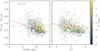 |
Fig. 16. Relationships between m3.6 − m4.5 color and stellar mass (left panel) or concentration (right panel). The dashed red lines show linear fits to the ETG populations only, while dotted black lines shows fits to the LTGs. ETG data points are multicolored, while LTGs are shown in gray. |
In the right panel of Fig. 16, we show the correlation between integrated m3.6 − m4.5 color and the concentration parameter C82 (Eq. (6)). This shows a similar blueward trend (red dashed line; ρ = −0.120, p = 2.67 × 10⁻¹⁰) as the stellar mass correlation, as expected given that C82 correlates already with stellar mass (Fig. 7). Again, LTGs show no significant correlation. They do, however, fall at the tail end of the ETG correlation, appearing as a cloud of points near C82 ∼ 2.6 (corresponding to n = 1). Indeed, a fit to the entire population of S4G+ETG galaxies gives a very similar slope to the ETG fit alone (−0.024 and −0.025, respectively). Meidt et al. (2014) also found that metallicity had the strongest impact on dust-free synthetic stellar population colors, due to CO absorption in the photospheres of giant stars (echoing Peletier et al. 2012, and references therein). Given their lower masses (Fig. 6), LTGs are also on average lower in metallicity (e.g., Tremonti et al. 2004; Gallazzi et al. 2005), so this may be primarily what is driving this behavior. A simple calculation provides evidence for this. From our linear fit

we can predict the expected color difference between the two populations. The median value of C82 for ETGs is 4.40 (Sect. 4), while that of LTGs is 2.96, yielding a difference in C82 of 1.44. The expected color difference from Eq. (20) is thus −0.025 × 1.44 ≈ −0.04 mag. The median color of the ETG sample is −0.48 mag, while that of the LTG sample is −0.42 mag, yielding a median color difference of −0.06 mag, slightly redward from the expectation from the linear relation. If age has little impact on these colors in uncontaminated stellar photosphere emission, the remaining ∼0.02 mag color difference could be attributable to nonstellar emission, which Meidt et al. (2012) showed has a fairly small impact on integrated quantities (of order 10% on stellar mass estimates, for example).
In summary, we replicate the blue-ward m3.6 − m4.5 color trend with stellar mass among ETGs using integrated magnitudes, in contrast to the LTG population, which shows no color trend with mass. This trend leads to a color-concentration relation as well, with LTGs occupying the low-concentration, red-color end of the entire S4G+ETG population, when metallicity and dust effects are taken into consideration.
6. Data online access
As for the initial S4G results (MM2015; Salo et al. 2015; Querejeta et al. 2015), all of our data will be made available online at a dedicated webpage at the NASA/IPAC Infrared Science Archive. We will provide, for each galaxy, the P1 images and weight maps, the P2 masks, and the P3 radial profiles (as ASCII tables). Once they become available, we will also upload the P4 multicomponent decompositions and any additional pipeline products to this same location.
Additionally, we will make all of our derived parameters available in table format: asymptotic magnitudes in both photometric bands (and associated uncertainties), both apparent and absolute; concentration parameters in both photometric bands; stellar masses; distances; effective radii in both photometric bands; local sky estimates in both photometric bands (and associated uncertainties); isophotal radii (R25.5 and R26.5) in both photometric bands; isophotal parameters associated with these radii (position angles and ellipticities); and revised morphological classifications based on the 3.6 μm images. For the sake of reproducibility, we will also include the limits within which we made our linear fits for deriving our asymptotic magnitudes (drawn from the radial profiles). Also following MM2015, we are including ancillary values from NED and HyperLEDA5, including optical colors, gas content, internal kinematics, etc., if the user wishes to define specific subsamples selected according to specific criteria.
Finally, we will also make all of the above tables and FITS images available at the CDS.
7. Summary
We have presented the data release of the ETG extension to the S4G, an NIR survey of nearby galaxies in a wavelength regime (3.6 μm and 4.5 μm) that is a nearly direct tracer of stellar mass. This extension includes newly calibrated images of 465 nearby ETGs not observed during the original S4G. We have now processed these images up through Pipeline 3, which derives surface photometry and associated parameters for each galaxy. This includes radial surface brightness profiles, curves of growth, asymptotic magnitudes (converted as well to stellar masses), effective radii, isophotal radii, and concentration parameters. We also include updated CVRHS morphological classifications for these ETGs.
Using these parameters, we have conducted a preliminary investigation into the following scaling relations:
-
Stellar mass-concentration, in which we show that S0 and elliptical galaxies follow roughly the same correlation, though disk galaxies tend to scatter to lower concentrations at a given stellar mass (which is also true of LTGs). We also demonstrate that single-component fits to ETGs tend to underestimate concentration by overestimating the luminosity of the galaxies’ outskirts. This results in single-component magnitudes that are slightly too bright compared to their empirical counterparts; multicomponent fits are necessary even for these otherwise visually simple elliptical galaxies.
-
Stellar mass-size, including both effective and isophotal radius. We find good agreement with past measures of the mass-effective radius relation for ETGs at z = 0, taking into account methodological differences. We find that the corresponding isophotal radius relation has surprisingly low scatter once galaxy inclination is corrected for, including among the more pressure-supported, triaxial ellipticals.
-
Surface brightness profile shape, including relations between stellar mass and central surface brightness, median surface brightness within the effective radius, and median surface brightness within 1 kpc radius. Surface brightness profiles of high-mass ETGs are brighter and, when normalized by effective radius, more extended than those of low-mass ETGs, but there is no noticeable trend with ETG morphological class. We reproduce the log-linear mass-central surface brightness trend found by other studies, but we note that, as with concentration parameters, single-component fits used to estimate this tend to fall short in galaxies with complex structure, often leading to extreme fitted Sérsic indices. The tightest of these surface brightness scaling relations is between stellar mass and surface brightness within 1 kpc, with little variation even between ETGs and LTGs, suggesting that the central 1 kpc of most galaxies is only mildly affected by whatever processes lead to morphological differentiation over cosmic time.
-
Stellar mass-NIR color, in which we reproduce the tendency for m3.6 − m4.5 to become bluer for higher-mass galaxies, a result of a CO absorption feature in the 4.5 μm band. This trend is echoed in the concentration-color relation, where LTGs form roughly the low-concentration, reddest color tail of the ETG trend.
Altogether, our preliminary look into these scaling relations shows good agreement with those of previous studies, but also includes some details that are worthy of further investigations. All of these images, profiles, and derived parameters will be made available via the NASA/IPAC Infrared Science Archive, and at the CDS.
The galaxies shown in Fig. 13 in Venhola et al. (2018) are mainly background galaxies at distances much larger than the 20 Mpc distance of the Fornax Cluster, making the resolution a more pronounced problem than for our sample, even if the FWHM of the FDS observations was smaller (about 1″ instead our Spitzer 2″).
Acknowledgments
AW acknowledges support from the STFC [ST/S00615X/1]. SC acknowledges funding from the State Research Agency (AEI-MCINN) of the Spanish Ministry of Science and Innovation under the grants “The structure and evolution of galaxies and their central regions” with reference PID2019-105602GB-I00/10.13039/501100011033, and “Thick discs, relics of the infancy of galaxies" with reference PID2020-113213GA-I00. This project has received funding from the European Union’s Horizon 2020 research and innovation programme under the Marie Skłodowska-Curie grant agreement No. 893673 (SDG), as well as grant agreement No. 721463 to the SUNDIAL ITN network (AHS, HS, JHK), from the State Research Agency (AEI-MCINN) of the Spanish Ministry of Science and Innovation under the grant “The structure and evolution of galaxies and their central regions” with reference PID2019-105602GB-I00/10.13039/501100011033, and from the IAC project P/300724 which is financed by the Ministry of Science and Innovation, through the State Budget and by the Canary Islands Department of Economy, Knowledge and Employment, through the Regional Budget of the Autonomous Community. EA and AB gratefully acknowledge financial support from CNES (Centre National d’Études Spatiales, France). LCH is supported by the National Science Foundation of China (11721303 and 11991052) and the National Key R&D Program of China (2016YFA0400702). TK acknowledges support from the Basic Science Research Program through the National Research Foundation of Korea (NRF) funded by the Ministry of Education (NRF-2019R1I1A3A02062242). KMD thanks the support of the Serrapilheira Institute (grant Serra-1709-17357) as well as that of the Brazilian National Council for Scientific and Technological Development (CNPq grant 312702/2017-5) and of the Carlos Chagas Filho Foundation for Supporting Research in the State of Rio de Janeiro (FAPERJ grant E-26/203.184/2017), Brazil. This work is based on observations made with the Spitzer Space Telescope, which was operated by the Jet Propulsion Laboratory, California Institute of Technology under a contract with NASA. Support for this work was provided by NASA through an award issued by JPL/Caltech. This research has made use of the NASA/IPAC Extragalactic Database (NED), which is funded by the National Aeronautics and Space Administration and operated by the California Institute of Technology. This work made use of the Python packages Numpy (Harris et al. 2020), Scipy (Virtanen et al. 2020), and Matplotlib (Hunter 2007). We thank Jarkko Laine for providing us with some of the IRAF scripts used to produce the radial profiles discussed in MM2015, which were critical to us for keeping the methodology consistent across such a gap of time. Finally, we thank the anonymous referee for their valuable feedback.
References
- Abraham, R. G., Valdes, F., Yee, H. K. C., & van den Bergh, S. 1994, ApJ, 432, 75 [NASA ADS] [CrossRef] [Google Scholar]
- Aguerri, J. A. L. 2012, Adv. Astron., 2012, 382674 [NASA ADS] [CrossRef] [Google Scholar]
- Aguerri, J. A. L., Balcells, M., & Peletier, R. F. 2001, A&A, 367, 428 [NASA ADS] [CrossRef] [EDP Sciences] [Google Scholar]
- Aguerri, J. A. L., Elias-Rosa, N., Corsini, E. M., & Muñoz-Tuñón, C. 2005, A&A, 434, 109 [NASA ADS] [CrossRef] [EDP Sciences] [Google Scholar]
- Aihara, H., Armstrong, R., Bickerton, S., et al. 2018, PASJ, 70, S8 [NASA ADS] [Google Scholar]
- Allers, K. N., Jaffe, D. T., van der Bliek, N. S., Allard, F., & Baraffe, I. 2006, in The Spitzer Space Telescope: New Views of the Cosmos, eds. L. Armus, & W. T. Reach, ASP Conf. Ser., 357, 77 [NASA ADS] [Google Scholar]
- Andreon, S., Dong, H., & Raichoor, A. 2016, A&A, 593, A2 [NASA ADS] [CrossRef] [EDP Sciences] [Google Scholar]
- Arora, N., Stone, C., Courteau, S., & Jarrett, T. H. 2021, MNRAS, 505, 3135 [NASA ADS] [CrossRef] [Google Scholar]
- Athanassoula, E. 1992, MNRAS, 259, 345 [Google Scholar]
- Athanassoula, E. 2003, MNRAS, 341, 1179 [Google Scholar]
- Athanassoula, E. 2005, MNRAS, 358, 1477 [NASA ADS] [CrossRef] [Google Scholar]
- Athanassoula, E., Lambert, J. C., & Dehnen, W. 2005, MNRAS, 363, 496 [Google Scholar]
- Athanassoula, E., Romero-Gómez, M., Bosma, A., & Masdemont, J. J. 2010, MNRAS, 407, 1433 [NASA ADS] [CrossRef] [Google Scholar]
- Athanassoula, E., Rodionov, S. A., Peschken, N., & Lambert, J. C. 2016, ApJ, 821, 90 [NASA ADS] [CrossRef] [Google Scholar]
- Balcells, M., Aguerri, J. A. L., & Peletier, R. F. 2003, in The Mass of Galaxies at Low and High Redshift, eds. R. Bender, & A. Renzini, 97 [CrossRef] [Google Scholar]
- Baldry, I. K., Glazebrook, K., Brinkmann, J., et al. 2004, ApJ, 600, 681 [Google Scholar]
- Barnes, J. E. 1988, ApJ, 331, 699 [NASA ADS] [CrossRef] [Google Scholar]
- Barnes, J. E. 1990, Nature, 344, 379 [NASA ADS] [CrossRef] [Google Scholar]
- Begelman, M. C., Blandford, R. D., & Rees, M. J. 1980, Nature, 287, 307 [Google Scholar]
- Bekki, K., Couch, W. J., & Shioya, Y. 2002, ApJ, 577, 651 [Google Scholar]
- Bendo, G. J., & Barnes, J. E. 2000, MNRAS, 316, 315 [Google Scholar]
- Bershady, M. A., Jangren, A., & Conselice, C. J. 2000, AJ, 119, 2645 [NASA ADS] [CrossRef] [Google Scholar]
- Bertin, E., & Arnouts, S. 1996, A&AS, 117, 393 [NASA ADS] [CrossRef] [EDP Sciences] [Google Scholar]
- Bertola, F., & Capaccioli, M. 1975, ApJ, 200, 439 [NASA ADS] [CrossRef] [Google Scholar]
- Bezanson, R., van Dokkum, P. G., Tal, T., et al. 2009, ApJ, 697, 1290 [Google Scholar]
- Binggeli, B., & Cameron, L. M. 1991, A&A, 252, 27 [NASA ADS] [Google Scholar]
- Binggeli, B., Sandage, A., & Tammann, G. A. 1985, AJ, 90, 1681 [Google Scholar]
- Binney, J. 1978, MNRAS, 183, 501 [NASA ADS] [Google Scholar]
- Bonanos, A. Z., Massa, D. L., Sewilo, M., et al. 2009, AJ, 138, 1003 [Google Scholar]
- Bonanos, A. Z., Lennon, D. J., Köhlinger, F., et al. 2010, AJ, 140, 416 [NASA ADS] [CrossRef] [Google Scholar]
- Boselli, A., Boissier, S., Cortese, L., & Gavazzi, G. 2008, A&A, 489, 1015 [CrossRef] [EDP Sciences] [Google Scholar]
- Bouquin, A. Y. K., Gil de Paz, A., Muñoz-Mateos, J. C., et al. 2018, ApJS, 234, 18 [NASA ADS] [CrossRef] [Google Scholar]
- Bournaud, F., Jog, C. J., & Combes, F. 2007, A&A, 476, 1179 [NASA ADS] [CrossRef] [EDP Sciences] [Google Scholar]
- Buitrago, F., Trujillo, I., Conselice, C. J., et al. 2008, ApJ, 687, L61 [Google Scholar]
- Burstein, D., Ho, L. C., Huchra, J. P., & Macri, L. M. 2005, ApJ, 621, 246 [NASA ADS] [CrossRef] [Google Scholar]
- Busko, I. C. 1996, in Astronomical Data Analysis Software and Systems V, eds. G. H. Jacoby, & J. Barnes, ASP Conf. Ser., 101, 139 [Google Scholar]
- Buta, R., & Combes, F. 1996, Fund. Cosmic Phys., 17, 95 [Google Scholar]
- Buta, R. J., Corwin, H. G., & Odewahn, S. C. 2007, The de Vaucouleurs Atlas of Galaxies (Cambridge, UK: Cambridge University Press) [Google Scholar]
- Buta, R. J., Sheth, K., Regan, M., et al. 2010, ApJS, 190, 147 [CrossRef] [Google Scholar]
- Buta, R. J., Sheth, K., Athanassoula, E., et al. 2015, ApJS, 217, 32 [Google Scholar]
- Calvi, R., Poggianti, B. M., Fasano, G., & Vulcani, B. 2012, MNRAS, 419, L14 [NASA ADS] [CrossRef] [Google Scholar]
- Calzetti, D. 2001, PASP, 113, 1449 [Google Scholar]
- Caon, N., Capaccioli, M., & D’Onofrio, M. 1993, MNRAS, 265, 1013 [NASA ADS] [CrossRef] [Google Scholar]
- Cappellari, M. 2016, ARA&A, 54, 597 [Google Scholar]
- Cappellari, M., Emsellem, E., Bacon, R., et al. 2007, MNRAS, 379, 418 [Google Scholar]
- Cappellari, M., Emsellem, E., Krajnović, D., et al. 2011a, MNRAS, 413, 813 [Google Scholar]
- Cappellari, M., Emsellem, E., Krajnović, D., et al. 2011b, MNRAS, 416, 1680 [Google Scholar]
- Carles, C., Martel, H., Ellison, S. L., & Kawata, D. 2016, MNRAS, 463, 1074 [NASA ADS] [CrossRef] [Google Scholar]
- Chamba, N., Trujillo, I., & Knapen, J. H. 2020, A&A, 633, L3 [NASA ADS] [CrossRef] [EDP Sciences] [Google Scholar]
- Cohen, M., Witteborn, F. C., Bregman, J. D., et al. 1996, AJ, 112, 241 [NASA ADS] [CrossRef] [Google Scholar]
- Combes, F., & Sanders, R. H. 1981, A&A, 96, 164 [NASA ADS] [Google Scholar]
- Comerón, S. 2013, A&A, 555, L4 [NASA ADS] [CrossRef] [EDP Sciences] [Google Scholar]
- Comerón, S., Elmegreen, B. G., Knapen, J. H., et al. 2011, ApJ, 741, 28 [CrossRef] [Google Scholar]
- Comerón, S., Salo, H., Peletier, R. F., & Mentz, J. 2016, A&A, 593, L6 [NASA ADS] [CrossRef] [EDP Sciences] [Google Scholar]
- Comerón, S., Salo, H., & Knapen, J. H. 2018, A&A, 610, A5 [NASA ADS] [CrossRef] [EDP Sciences] [Google Scholar]
- Conselice, C. J. 2003, ApJS, 147, 1 [NASA ADS] [CrossRef] [Google Scholar]
- Conselice, C. J. 2006, MNRAS, 373, 1389 [NASA ADS] [CrossRef] [Google Scholar]
- Corsini, E. M., Wegner, G. A., Thomas, J., Saglia, R. P., & Bender, R. 2017, MNRAS, 466, 974 [Google Scholar]
- Côté, P., Piatek, S., Ferrarese, L., et al. 2006, ApJS, 165, 57 [Google Scholar]
- Daddi, E., Renzini, A., Pirzkal, N., et al. 2005, ApJ, 626, 680 [NASA ADS] [CrossRef] [Google Scholar]
- Davari, R. H., Ho, L. C., Mobasher, B., & Canalizo, G. 2017, ApJ, 836, 75 [NASA ADS] [CrossRef] [Google Scholar]
- Davies, R. L., & Illingworth, G. 1983, ApJ, 266, 516 [NASA ADS] [CrossRef] [Google Scholar]
- Davies, R. L., Efstathiou, G., Fall, S. M., Illingworth, G., & Schechter, P. L. 1983, ApJ, 266, 41 [NASA ADS] [CrossRef] [Google Scholar]
- de Vaucouleurs, G. 1948, Ann. Astrophys., 11, 247 [Google Scholar]
- de Vaucouleurs, G. 1959, Handbuch der Physik, 53, 275 [Google Scholar]
- de Vaucouleurs, G. 1977, in Evolution of Galaxies and Stellar Populations, eds. B. M. Tinsley, D. C. Larson, & R. B. Gehret, 43 [Google Scholar]
- de Vaucouleurs, G., & Agüero, E. 1973, PASP, 85, 150 [NASA ADS] [CrossRef] [Google Scholar]
- de Vaucouleurs, G., de Vaucouleurs, A., Corwin, H. G. J., et al. 1991, Third Reference Catalogue of Bright Galaxies (New York, NY USA: Springer) [Google Scholar]
- de Zeeuw, T., & Franx, M. 1991, ARA&A, 29, 239 [NASA ADS] [CrossRef] [Google Scholar]
- Debattista, V. P., Mayer, L., Carollo, C. M., et al. 2006, ApJ, 645, 209 [Google Scholar]
- den Brok, M., Peletier, R. F., Valentijn, E. A., et al. 2011, MNRAS, 414, 3052 [Google Scholar]
- Díaz-García, S., Salo, H., & Laurikainen, E. 2016, A&A, 596, A84 [NASA ADS] [CrossRef] [EDP Sciences] [Google Scholar]
- Díaz-García, S., Salo, H., Knapen, J. H., & Herrera-Endoqui, M. 2019, A&A, 631, A94 [CrossRef] [EDP Sciences] [Google Scholar]
- Djorgovski, S., & Davis, M. 1987, ApJ, 313, 59 [Google Scholar]
- Draine, B. T., & Lee, H. M. 1984, ApJ, 285, 89 [NASA ADS] [CrossRef] [Google Scholar]
- Dressler, A. 1980, ApJ, 236, 351 [Google Scholar]
- Dressler, A., Lynden-Bell, D., Burstein, D., et al. 1987, ApJ, 313, 42 [Google Scholar]
- Driver, S. P., Wright, A. H., Andrews, S. K., et al. 2016, MNRAS, 455, 3911 [NASA ADS] [CrossRef] [Google Scholar]
- Dullo, B. T., & Graham, A. W. 2012, ApJ, 755, 163 [NASA ADS] [CrossRef] [Google Scholar]
- Ebisuzaki, T., Makino, J., & Okumura, S. K. 1991, Nature, 354, 212 [NASA ADS] [CrossRef] [Google Scholar]
- Eggen, O. J., Lynden-Bell, D., & Sandage, A. R. 1962, ApJ, 136, 748 [NASA ADS] [CrossRef] [Google Scholar]
- Eliche-Moral, M. C., Borlaff, A., Beckman, J. E., & Gutiérrez, L. 2015, A&A, 580, A33 [NASA ADS] [CrossRef] [EDP Sciences] [Google Scholar]
- Emsellem, E., Cappellari, M., Krajnović, D., et al. 2007, MNRAS, 379, 401 [Google Scholar]
- Emsellem, E., Cappellari, M., Krajnović, D., et al. 2011, MNRAS, 414, 888 [Google Scholar]
- Erwin, P., Pohlen, M., & Beckman, J. E. 2008, AJ, 135, 20 [Google Scholar]
- Eskew, M., Zaritsky, D., & Meidt, S. 2012, AJ, 143, 139 [NASA ADS] [CrossRef] [Google Scholar]
- Faber, S. M., Tremaine, S., Ajhar, E. A., et al. 1997, AJ, 114, 1771 [NASA ADS] [CrossRef] [Google Scholar]
- Falcón-Barroso, J., van de Ven, G., Lyubenova, M., et al. 2019, A&A, 632, A59 [Google Scholar]
- Fathi, K., & Peletier, R. F. 2003, A&A, 407, 61 [NASA ADS] [CrossRef] [EDP Sciences] [Google Scholar]
- Fazio, G. G., Hora, J. L., Allen, L. E., et al. 2004, ApJS, 154, 10 [Google Scholar]
- Ferrarese, L., Côté, P., Jordán, A., et al. 2006, ApJS, 164, 334 [NASA ADS] [CrossRef] [Google Scholar]
- Fliri, J., & Trujillo, I. 2016, MNRAS, 456, 1359 [Google Scholar]
- Fraser, C. W. 1972, The Observatory, 92, 51 [NASA ADS] [Google Scholar]
- Frenk, C. S., White, S. D. M., Efstathiou, G., & Davis, M. 1985, Nature, 317, 595 [NASA ADS] [CrossRef] [Google Scholar]
- Fruchter, A. S., & Hook, R. N. 2002, PASP, 114, 144 [NASA ADS] [CrossRef] [Google Scholar]
- Gallazzi, A., Charlot, S., Brinchmann, J., White, S. D. M., & Tremonti, C. A. 2005, MNRAS, 362, 41 [Google Scholar]
- Gott, J. R. I. 1973, ApJ, 186, 481 [NASA ADS] [CrossRef] [Google Scholar]
- Gott, J. R. I. 1977, ARA&A, 15, 235 [NASA ADS] [CrossRef] [Google Scholar]
- Graham, A. W. 2001, AJ, 121, 820 [NASA ADS] [CrossRef] [Google Scholar]
- Graham, A. W. 2019, PASA, 36, e035 [NASA ADS] [CrossRef] [Google Scholar]
- Graham, A. W., & Driver, S. P. 2005, PASA, 22, 118 [NASA ADS] [CrossRef] [Google Scholar]
- Graham, A. W., & Guzmán, R. 2003, AJ, 125, 2936 [Google Scholar]
- Graham, A. W., Trujillo, I., & Caon, N. 2001, AJ, 122, 1707 [NASA ADS] [CrossRef] [Google Scholar]
- Gudehus, D. H. 1973, AJ, 78, 583 [NASA ADS] [CrossRef] [Google Scholar]
- Gunn, J. E., Gott, J., & Richard, I. 1972, ApJ, 176, 1 [Google Scholar]
- Hall, M., Courteau, S., Dutton, A. A., McDonald, M., & Zhu, Y. 2012, MNRAS, 425, 2741 [Google Scholar]
- Harris, C. R., Millman, K. J., van der Walt, S. J., et al. 2020, Nature, 585, 357 [NASA ADS] [CrossRef] [Google Scholar]
- Hernquist, L. 1992, ApJ, 400, 460 [NASA ADS] [CrossRef] [Google Scholar]
- Herrera-Endoqui, M., Díaz-García, S., Laurikainen, E., & Salo, H. 2015, A&A, 582, A86 [NASA ADS] [CrossRef] [EDP Sciences] [Google Scholar]
- Holwerda, B. W., Muñoz-Mateos, J. C., Comerón, S., et al. 2014, ApJ, 781, 12 [Google Scholar]
- Hopkins, P. F., Cox, T. J., & Hernquist, L. 2008, ApJ, 689, 17 [NASA ADS] [CrossRef] [Google Scholar]
- Hopkins, P. F., Bundy, K., Murray, N., et al. 2009, MNRAS, 398, 898 [Google Scholar]
- Hora, J. L., Marengo, M., Park, R., et al. 2012, in Space Telescopes and Instrumentation 2012: Optical, Infrared, and Millimeter Wave, eds. M. C. Clampin, G. G. Fazio, H. A. MacEwen, J. Oschmann, & M. Jacobus, SPIE Conf. Ser., 8842, 844239 [NASA ADS] [CrossRef] [Google Scholar]
- Hubble, E. P. 1926, ApJ, 64, 321 [Google Scholar]
- Hunter, J. D. 2007, Comput. Sci. Eng., 9, 90 [NASA ADS] [CrossRef] [Google Scholar]
- İkz, T., Peletier, R. F., Barthel, P. D., & Yeşilyaprak, C. 2020, A&A, 640, A68 [CrossRef] [EDP Sciences] [Google Scholar]
- Illingworth, G. 1977, ApJ, 218, L43 [Google Scholar]
- Impey, C. D., Sprayberry, D., Irwin, M. J., & Bothun, G. D. 1996, ApJS, 105, 209 [Google Scholar]
- Iodice, E., Cantiello, M., Hilker, M., et al. 2020, A&A, 642, A48 [EDP Sciences] [Google Scholar]
- Ivezić, Ž., Kahn, S. M., Tyson, J. A., et al. 2019, ApJ, 873, 111 [Google Scholar]
- Janz, J., & Lisker, T. 2008, ApJ, 689, L25 [Google Scholar]
- Janz, J., Laurikainen, E., Lisker, T., et al. 2014, ApJ, 786, 105 [Google Scholar]
- Jarrett, T. H., Chester, T., Cutri, R., Schneider, S. E., & Huchra, J. P. 2003, AJ, 125, 525 [Google Scholar]
- Jarrett, T. H., Masci, F., Tsai, C. W., et al. 2013, AJ, 145, 6 [Google Scholar]
- Jedrzejewski, R. I. 1987, MNRAS, 226, 747 [Google Scholar]
- Jun, H. D., & Im, M. 2008, ApJ, 678, L97 [CrossRef] [Google Scholar]
- Kaneda, H., Onaka, T., & Sakon, I. 2007, ApJ, 666, L21 [NASA ADS] [CrossRef] [Google Scholar]
- Karachentsev, I. D., Makarov, D. I., Karachentseva, V. E., & Melnyk, O. V. 2010, in Galaxies in Isolation: Exploring Nature Versus Nurture, eds. L. Verdes-Montenegro, A. Del Olmo, & J. Sulentic, ASP Conf. Ser., 421, 69 [NASA ADS] [Google Scholar]
- Kataria, S. K., Das, M., & Barway, S. 2020, A&A, 640, A14 [NASA ADS] [CrossRef] [EDP Sciences] [Google Scholar]
- Katkov, I. Y., Kniazev, A. Y., Kasparova, A. V., & Sil’chenko, O. K. 2019, MNRAS, 483, 2413 [NASA ADS] [CrossRef] [Google Scholar]
- Kauffmann, G., White, S. D. M., & Guiderdoni, B. 1993, MNRAS, 264, 201 [Google Scholar]
- Kauffmann, G., White, S. D. M., Heckman, T. M., et al. 2004, MNRAS, 353, 713 [Google Scholar]
- Kent, S. M. 1985, ApJS, 59, 115 [NASA ADS] [CrossRef] [Google Scholar]
- Kim, T., Sheth, K., Hinz, J. L., et al. 2012, ApJ, 753, 43 [NASA ADS] [CrossRef] [Google Scholar]
- Kim, T., Gadotti, D. A., Athanassoula, E., et al. 2016, MNRAS, 462, 3430 [Google Scholar]
- King, I. R., & Minkowski, R. 1966, ApJ, 143, 1002 [NASA ADS] [CrossRef] [Google Scholar]
- Koda, J., Yagi, M., Yamanoi, H., & Komiyama, Y. 2015, ApJ, 807, L2 [NASA ADS] [CrossRef] [Google Scholar]
- Kormendy, J. 1977, ApJ, 218, 333 [NASA ADS] [CrossRef] [Google Scholar]
- Kormendy, J. 1982, ApJ, 257, 75 [NASA ADS] [CrossRef] [Google Scholar]
- Kormendy, J. 1999, in Galaxy Dynamics– A Rutgers Symposium, eds. D. R. Merritt, M. Valluri, & J. A. Sellwood, ASP Conf. Ser., 182, 124 [Google Scholar]
- Kormendy, J., & Bender, R. 1996, ApJ, 464, L119 [NASA ADS] [CrossRef] [Google Scholar]
- Kormendy, J., & Bender, R. 2012, ApJS, 198, 2 [Google Scholar]
- Kormendy, J., & Kennicutt, R. C. J. 2004, ARA&A, 42, 603 [NASA ADS] [CrossRef] [Google Scholar]
- Kormendy, J., Fisher, D. B., Cornell, M. E., & Bender, R. 2009, ApJS, 182, 216 [Google Scholar]
- Krajnović, D. 2015, in Galaxy Masses as Constraints of Formation Models, eds. M. Cappellari, & S. Courteau, 311, 45 [Google Scholar]
- Krajnović, D., Ural, U., Kuntschner, H., et al. 2020, A&A, 635, A129 [NASA ADS] [CrossRef] [EDP Sciences] [Google Scholar]
- La Barbera, F., Merluzzi, P., Busarello, G., Massarotti, M., & Mercurio, A. 2004, A&A, 425, 797 [NASA ADS] [CrossRef] [EDP Sciences] [Google Scholar]
- Laine, S., Knapen, J. H., Muñoz-Mateos, J.-C., et al. 2014, MNRAS, 444, 3015 [NASA ADS] [CrossRef] [Google Scholar]
- Laine, J., Laurikainen, E., & Salo, H. 2016, A&A, 596, A25 [NASA ADS] [CrossRef] [EDP Sciences] [Google Scholar]
- Larson, R. B. 1974a, MNRAS, 166, 585 [NASA ADS] [CrossRef] [Google Scholar]
- Larson, R. B. 1974b, MNRAS, 169, 229 [NASA ADS] [CrossRef] [Google Scholar]
- Larson, R. B. 1975, MNRAS, 173, 671 [NASA ADS] [CrossRef] [Google Scholar]
- Lauer, T. R., Gebhardt, K., Faber, S. M., et al. 2007, ApJ, 664, 226 [Google Scholar]
- Laureijs, R. J., Duvet, L., Escudero Sanz, I., et al. 2010, Proc. SPIE, 7731, 77311H [NASA ADS] [CrossRef] [Google Scholar]
- Laurikainen, E., & Salo, H. 2017, A&A, 598, A10 [NASA ADS] [CrossRef] [EDP Sciences] [Google Scholar]
- Laurikainen, E., Salo, H., Buta, R., & Knapen, J. H. 2007, MNRAS, 381, 401 [Google Scholar]
- Laurikainen, E., Salo, H., Buta, R., Knapen, J. H., & Comerón, S. 2010, MNRAS, 405, 1089 [NASA ADS] [Google Scholar]
- Laurikainen, E., Salo, H., Buta, R., & Knapen, J. H. 2011, Adv. Astron., 2011 [CrossRef] [Google Scholar]
- Laurikainen, E., Salo, H., Athanassoula, E., et al. 2013, MNRAS, 430, 3489 [NASA ADS] [CrossRef] [Google Scholar]
- Longhetti, M., Saracco, P., Severgnini, P., et al. 2007, MNRAS, 374, 614 [NASA ADS] [CrossRef] [Google Scholar]
- Luhman, K. L., Hernández, J., Downes, J. J., Hartmann, L., & Briceño, C. 2008, ApJ, 688, 362 [NASA ADS] [CrossRef] [Google Scholar]
- Maciejewski, W., Teuben, P. J., Sparke, L. S., & Stone, J. M. 2002, MNRAS, 329, 502 [NASA ADS] [CrossRef] [Google Scholar]
- Mahajan, S., Drinkwater, M. J., Driver, S., et al. 2015, MNRAS, 446, 2967 [NASA ADS] [CrossRef] [Google Scholar]
- Martín-Navarro, I., Bakos, J., Trujillo, I., et al. 2012, MNRAS, 427, 1102 [Google Scholar]
- Meidt, S. E., Schinnerer, E., Knapen, J. H., et al. 2012, ApJ, 744, 17 [NASA ADS] [CrossRef] [Google Scholar]
- Meidt, S. E., Schinnerer, E., van de Ven, G., et al. 2014, ApJ, 788, 144 [Google Scholar]
- Méndez-Abreu, J., de Lorenzo-Cáceres, A., & Sánchez, S. F. 2021, MNRAS, 504, 3058 [CrossRef] [Google Scholar]
- Mihos, J. C., & Hernquist, L. 1994, ApJ, 437, L47 [NASA ADS] [CrossRef] [Google Scholar]
- Mihos, J. C., Durrell, P. R., Ferrarese, L., et al. 2015, ApJ, 809, L21 [Google Scholar]
- Milosavljević, M., & Merritt, D. 2001, ApJ, 563, 34 [Google Scholar]
- Moore, B., Katz, N., Lake, G., Dressler, A., & Oemler, A. 1996, Nature, 379, 613 [Google Scholar]
- Morgan, W. W. 1958, PASP, 70, 364 [NASA ADS] [CrossRef] [Google Scholar]
- Morgan, W. W., & Mayall, N. U. 1957, PASP, 69, 291 [NASA ADS] [CrossRef] [Google Scholar]
- Mould, J., Barmby, P., Gordon, K., et al. 2008, ApJ, 687, 230 [NASA ADS] [CrossRef] [Google Scholar]
- Muñoz-Mateos, J. C., Sheth, K., Gil de Paz, A., et al. 2013, ApJ, 771, 59 [Google Scholar]
- Muñoz-Mateos, J. C., Sheth, K., Regan, M., et al. 2015, ApJS, 219, 3 [Google Scholar]
- Naab, T., Johansson, P. H., & Ostriker, J. P. 2009, ApJ, 699, L178 [Google Scholar]
- Newman, A. B., Ellis, R. S., Bundy, K., & Treu, T. 2012, ApJ, 746, 162 [NASA ADS] [CrossRef] [Google Scholar]
- Nipoti, C., Londrillo, P., & Ciotti, L. 2003, MNRAS, 342, 501 [Google Scholar]
- Norman, C. A., Sellwood, J. A., & Hasan, H. 1996, ApJ, 462, 114 [NASA ADS] [CrossRef] [Google Scholar]
- Oemler, A. J. 1974, ApJ, 194, 1 [NASA ADS] [CrossRef] [Google Scholar]
- Okamura, S., Kodaira, K., & Watanabe, M. 1984, ApJ, 280, 7 [NASA ADS] [CrossRef] [Google Scholar]
- Oke, J. B. 1974, ApJS, 27, 21 [Google Scholar]
- Ouellette, N. N. Q., Courteau, S., Holtzman, J. A., et al. 2017, ApJ, 843, 74 [Google Scholar]
- Pahre, M. A., Ashby, M. L. N., Fazio, G. G., & Willner, S. P. 2004, ApJS, 154, 235 [NASA ADS] [CrossRef] [Google Scholar]
- Paturel, G., Petit, C., Prugniel, P., et al. 2003, A&A, 412, 45 [NASA ADS] [CrossRef] [EDP Sciences] [Google Scholar]
- Peletier, R. F., Davies, R. L., Illingworth, G. D., Davis, L. E., & Cawson, M. 1990, AJ, 100, 1091 [Google Scholar]
- Peletier, R. F., Kutdemir, E., van der Wolk, G., et al. 2012, MNRAS, 419, 2031 [NASA ADS] [CrossRef] [Google Scholar]
- Peletier, R., Iodice, E., Venhola, A., et al. 2020, ArXiv e-prints [arXiv:2008.12633] [Google Scholar]
- Peng, C. Y., Ho, L. C., Impey, C. D., & Rix, H.-W. 2002, AJ, 124, 266 [Google Scholar]
- Peng, C. Y., Ho, L. C., Impey, C. D., & Rix, H.-W. 2010, AJ, 139, 2097 [Google Scholar]
- Petrosian, V. 1976, ApJ, 210, L53 [NASA ADS] [CrossRef] [Google Scholar]
- Pohlen, M., & Trujillo, I. 2006, A&A, 454, 759 [NASA ADS] [CrossRef] [EDP Sciences] [Google Scholar]
- Pozzetti, L., Bolzonella, M., Zucca, E., et al. 2010, A&A, 523, A13 [NASA ADS] [CrossRef] [EDP Sciences] [Google Scholar]
- Querejeta, M., Eliche-Moral, M. C., Tapia, T., et al. 2015, A&A, 579, L2 [NASA ADS] [CrossRef] [EDP Sciences] [Google Scholar]
- Ramos, B. H. F., Menéndez-Delmestre, K., Kim, T., & Sheth, K. 2015, Highlights Astron., 16, 333 [NASA ADS] [Google Scholar]
- Rautiainen, P., & Salo, H. 2000, A&A, 362, 465 [NASA ADS] [Google Scholar]
- Ravindranath, S., Ho, L. C., Peng, C. Y., Filippenko, A. V., & Sargent, W. L. W. 2001, AJ, 122, 653 [Google Scholar]
- Reach, W. T., Megeath, S. T., Cohen, M., et al. 2005, PASP, 117, 978 [NASA ADS] [CrossRef] [Google Scholar]
- Rizzo, F., Fraternali, F., & Iorio, G. 2018, MNRAS, 476, 2137 [Google Scholar]
- Román, J., & Trujillo, I. 2018, Res. Notes. Am. Astron. Soc., 2, 144 [Google Scholar]
- Saha, K., & Cortesi, A. 2018, ApJ, 862, L12 [NASA ADS] [CrossRef] [Google Scholar]
- Saintonge, A., & Spekkens, K. 2011, ApJ, 726, 77 [NASA ADS] [CrossRef] [Google Scholar]
- Salo, H., Laurikainen, E., Laine, J., et al. 2015, ApJS, 219, 4 [Google Scholar]
- Sánchez Almeida, J. 2020, MNRAS, 495, 78 [Google Scholar]
- Sandage, A. 1961, The Hubble Atlas of Galaxies [Google Scholar]
- Saracco, P., Gargiulo, A., & Longhetti, M. 2012, MNRAS, 422, 3107 [NASA ADS] [CrossRef] [Google Scholar]
- Saracco, P., Gargiulo, A., Ciocca, F., & Marchesini, D. 2017, A&A, 597, A122 [NASA ADS] [CrossRef] [EDP Sciences] [Google Scholar]
- Savorgnan, G., Graham, A. W., Marconi, A., et al. 2013, MNRAS, 434, 387 [NASA ADS] [CrossRef] [Google Scholar]
- Schaye, J. 2004, ApJ, 609, 667 [NASA ADS] [CrossRef] [Google Scholar]
- Schlafly, E. F., & Finkbeiner, D. P. 2011, ApJ, 737, 103 [Google Scholar]
- Schombert, J. M. 1986, ApJS, 60, 603 [NASA ADS] [CrossRef] [Google Scholar]
- Schombert, J. M. 2015, AJ, 150, 162 [NASA ADS] [CrossRef] [Google Scholar]
- Sedgwick, T. M., Baldry, I. K., James, P. A., & Kelvin, L. S. 2019, IAU Symp., 355, 2019 [Google Scholar]
- Sellwood, J. A. 1980, A&A, 89, 296 [NASA ADS] [Google Scholar]
- Sellwood, J. A., & Binney, J. J. 2002, MNRAS, 336, 785 [Google Scholar]
- Shen, S., Mo, H. J., White, S. D. M., et al. 2003, MNRAS, 343, 978 [NASA ADS] [CrossRef] [Google Scholar]
- Sheth, K., Elmegreen, D. M., Elmegreen, B. G., et al. 2008, ApJ, 675, 1141 [Google Scholar]
- Sheth, K., Regan, M., Hinz, J. L., et al. 2010, PASP, 122, 1397 [Google Scholar]
- Sheth, K., Armus, L., Athanassoula, E., et al. 2013, Not Dead Yet! Completing Spitzer’s Legacy with Early Type Galaxies, Spitzer Proposal [Google Scholar]
- Sil’chenko, O. 2013, Mem. Soc. Astron. It. Suppl., 25, 93 [Google Scholar]
- Skibba, R. A., Engelbracht, C. W., Dale, D., et al. 2011, ApJ, 738, 89 [NASA ADS] [CrossRef] [Google Scholar]
- Spergel, D., Gehrels, N., Baltay, C., et al. 2015, ArXiv e-prints [arXiv:1503.03757] [Google Scholar]
- Spitzer, L. J., & Baade, W. 1951, ApJ, 113, 413 [NASA ADS] [CrossRef] [Google Scholar]
- Szomoru, D., Franx, M., & van Dokkum, P. G. 2012, ApJ, 749, 121 [Google Scholar]
- Tacchella, S., Dekel, A., Carollo, C. M., et al. 2016, MNRAS, 458, 242 [NASA ADS] [CrossRef] [Google Scholar]
- Taylor-Mager, V. A., Conselice, C. J., Windhorst, R. A., & Jansen, R. A. 2007, ApJ, 659, 162 [NASA ADS] [CrossRef] [Google Scholar]
- Thomas, J., Jesseit, R., Saglia, R. P., et al. 2009, MNRAS, 393, 641 [Google Scholar]
- Thomas, J., Saglia, R. P., Bender, R., Erwin, P., & Fabricius, M. 2014, ApJ, 782, 39 [Google Scholar]
- Thuan, T. X. 1975, Nature, 257, 774 [NASA ADS] [CrossRef] [Google Scholar]
- Toft, S., van Dokkum, P., Franx, M., et al. 2007, ApJ, 671, 285 [CrossRef] [Google Scholar]
- Tokunaga, A. T., Sellgren, K., Smith, R. G., et al. 1991, ApJ, 380, 452 [CrossRef] [Google Scholar]
- Toomre, A. 1977, in Evolution of Galaxies and Stellar Populations, eds. B. M. Tinsley, D. C. Larson, & R. B. Gehret, 401 [Google Scholar]
- Tremonti, C. A., Heckman, T. M., Kauffmann, G., et al. 2004, ApJ, 613, 898 [Google Scholar]
- Trujillo, I., Graham, A. W., & Caon, N. 2001, MNRAS, 326, 869 [Google Scholar]
- Trujillo, I., Conselice, C. J., Bundy, K., et al. 2007, MNRAS, 382, 109 [NASA ADS] [CrossRef] [Google Scholar]
- Trujillo, I., Chamba, N., & Knapen, J. H. 2020, MNRAS, 493, 87 [NASA ADS] [CrossRef] [Google Scholar]
- van den Bergh, S. 1976, ApJ, 206, 883 [NASA ADS] [CrossRef] [Google Scholar]
- van den Bergh, S. 1998, Galaxy Morphology and Classification (Cambridge, NY USA: Cambridge University Press) [CrossRef] [Google Scholar]
- van der Wel, A. 2008, ApJ, 675, L13 [Google Scholar]
- van der Wel, A., Bell, E. F., van den Bosch, F. C., Gallazzi, A., & Rix, H.-W. 2009, ApJ, 698, 1232 [NASA ADS] [CrossRef] [Google Scholar]
- van der Wel, A., Franx, M., van Dokkum, P. G., et al. 2014, ApJ, 788, 28 [Google Scholar]
- van Dokkum, P. G., Franx, M., Kriek, M., et al. 2008, ApJ, 677, L5 [Google Scholar]
- van Dokkum, P. G., Abraham, R., Merritt, A., et al. 2015, ApJ, 798, L45 [NASA ADS] [CrossRef] [Google Scholar]
- Venhola, A., Peletier, R., Laurikainen, E., et al. 2018, A&A, 620, A165 [NASA ADS] [CrossRef] [EDP Sciences] [Google Scholar]
- Virtanen, P., Gommers, R., Oliphant, T. E., et al. 2020, Nat. Methods, 17, 261 [Google Scholar]
- Watkins, A. E., Laine, J., Comerón, S., Janz, J., & Salo, H. 2019, A&A, 625, A36 [NASA ADS] [CrossRef] [EDP Sciences] [Google Scholar]
- Wegner, G. A., Corsini, E. M., Thomas, J., et al. 2012, AJ, 144, 78 [Google Scholar]
- Werner, M. W., Roellig, T. L., Low, F. J., et al. 2004, ApJS, 154, 1 [NASA ADS] [CrossRef] [Google Scholar]
- White, S. D. M. 1983, in Internal Kinematics and Dynamics of Galaxies, ed. E. Athanassoula, IAU Symp., 100, 337 [NASA ADS] [CrossRef] [Google Scholar]
- White, S. D. M., & Rees, M. J. 1978, MNRAS, 183, 341 [Google Scholar]
- Williams, S. J., & Bonanos, A. Z. 2016, A&A, 587, A121 [NASA ADS] [CrossRef] [EDP Sciences] [Google Scholar]
- Willner, S. P., Soifer, B. T., Russell, R. W., Joyce, R. R., & Gillett, F. C. 1977, ApJ, 217, L121 [NASA ADS] [CrossRef] [Google Scholar]
- Wilman, D. J., & Erwin, P. 2012, ApJ, 746, 160 [NASA ADS] [CrossRef] [Google Scholar]
- Wyse, R. F. G., & Jones, B. J. T. 1984, ApJ, 286, 88 [NASA ADS] [CrossRef] [Google Scholar]
- Young, C. K., & Currie, M. J. 1994, MNRAS, 268, L11 [NASA ADS] [CrossRef] [Google Scholar]
- Zaritsky, D., Salo, H., Laurikainen, E., et al. 2013, ApJ, 772, 135 [Google Scholar]
- Zhu, Y.-N., Wu, H., Li, H.-N., & Cao, C. 2010, Res. Astron. Astrophys., 10, 329 [Google Scholar]
Appendix A: Updated ETG morphological classifications
We will make our updated CVRHS (Buta et al. 2007) morphological classifications (Sec. 2) for all of the newly observed ETGs in the S4G+ETG sample available at IPAC and at CDS, alongside all of the other quantities we have discussed in this paper. Table A.1 shows a subsample of the full table we will provide, which will contain morphological classifications for all 465 newly observed galaxies. This includes the full CVRHS classification, outer and inner structure classifications (rings, lenses, barlenses, etc.), the numerical family index corresponding to the presence or absence of a bar, and the numerical T-type (which we have used throughout this paper).
CVRHS classifications for newly observed S4G ETGs
All Tables
All Figures
|
Fig. 1. HyperLEDA T-type distribution (left panel) and T-type distribution from 3.6 μm classifications by R. Buta (right panel) for the 465 newly observed ETGs in the S4G+ETG sample. We use the Buta T-types for the remainder of this paper, given their improved accuracy. |
| In the text | |
|
Fig. 2. Showcasing examples of radial profiles, as described in Sect. 3.2, using NGC 720. Top left panel: the 3.6 μm image, with masks shown via the red contours. Bottom left panel: the same image, with 2″ radial bin width, variable PA and ϵ isophotal ellipses overlaid in black. The blue ellipse shows B-band R25 from HyperLEDA, while the two red ellipses show our values of R25.5, 3.6 and R26.5, 3.6 (solid and dashed, respectively). Rightmost panels: radial profiles of, from top to bottom: surface brightness, ellipticity, and position angle. The 3.6 μm and 4.5 μm profiles are offset from each other by the amounts shown in the legends to avoid significant overlap. Profiles shown here are truncated in radius compared to those available online, to avoid clutter from poor-quality fits in the far outskirts. Vertical dotted red lines show R25.5, 3.6. |
| In the text | |
|
Fig. 3. Demonstrating interpolation across masks for a heavily masked galaxy (IC 3381). Top panel: the masked image, while the bottom panel shows the same image but with the galaxy’s light interpolated azimuthally across the masked pixels (see Sect. 3.2). |
| In the text | |
|
Fig. 4. Comparing aperture corrections for a single radial surface brightness profile. Left panels: the effect of the aperture correction described by MM2015. The black line shows the unaltered surface brightness profile for NGC 720, while the gray line shows the same profile after the aperture correction is applied. Bottom left panel: the difference between the two (unaltered−corrected). Right panels are the same as the left panels but show our more robust aperture correction using GALFIT models (see Sect. 3.2). We derived all magnitudes and related quantities using the MM2015 correction, to maintain consistency with that study; however, for any future analysis using our data sets, we recommend instead using the revised correction. |
| In the text | |
|
Fig. 5. Example curves of growth for two galaxies, one bright with a large angular size (NGC 4564, left), the other faint with a small angular size (IC 271, right). Black points in the main panels show the total magnitudes enclosed within each radius (bin width 2″). The inset panels show the local gradients in the outskirts of the curves of growth. Red dashed lines show fits to the linear parts of these gradients chosen by eye; the y-intercepts of these red lines are the asymptotic magnitudes. Gray shaded regions show the 1σ (dark gray) and 2σ (light gray) perturbations to the curves of growth from adjusting the sky subtraction (see Sect. 3.3). |
| In the text | |
|
Fig. 6. Distributions of the photometric parameters discussed in Sect. 3 (top), and parameter values plotted against morphological T-type (bottom). From left to right: the parameters shown are: decimal logarithm of stellar mass (in solar units); concentration parameter C82 (Eq. (6)); concentration parameter C31 (Eq. (5)); logarithm of the μ3.6, AB = 25.5 mag arcsec−2 isophotal radius in kiloparsecs; and logarithm of the half-light (∼half-mass) radius in kiloparsecs. Solid red lines show the median value of each parameter measured in bins of ΔT = 1, while dashed red lines show the associated first and third quartiles. Unfilled histograms and gray points show distributions for all the galaxies, while filled histograms and black points show distributions for galaxies with T ≤ 0 and T = 11 (ETGs). |
| In the text | |
|
Fig. 7. Correlation between concentration and stellar mass. Here and in all subsequent figures with this color scheme, we show ETGs (T ≤ 0) color-coded by T-type, while we show all S4G galaxies in gray. We show dwarf ETGs (T = 11) in cyan. The dashed black line shows a linear fit between log (ℳ*/ℳ⊙) and log (n), converted from C82, for ETGs (Eq. (7)). The red dashed line shows a similar fit, but here n was estimated for each ETG via single-component 2D decompositions (Eq. (8)). |
| In the text | |
|
Fig. 8. Investigating the divergence between the Sérsic n derived from C82 and that measured from single-component 2D decompositions. Top-left panel: concentration parameter vs. Sérsic index, the latter being derived from single-component 2D decompositions for all S4G galaxies. The solid black line shows the theoretical behavior of C82 for Sérsic profiles of varying n. Here and in subsequent panels, the dashed black line shows the median of points in equal-width bins (bins with fewer than five points are ignored). Bottom-left panel: we show the difference between our asymptotic magnitudes and those derived from decompositions (negative numbers mean the asymptotic magnitudes are fainter). The solid black line here and in the following panels shows a value of 0 (no difference). Top-right panel: difference between R20 derived from single-component decompositions and those derived from our curves of growth for 3.6 μm imaging. The vertical dotted line shows the size of three IRAC 3.6 μm resolution elements. Bottom-right panel: the same as the top-right panel, but shows the behavior of R80. ETG data points are multicolored (with dwarfs in cyan), while LTGs are shown in gray. |
| In the text | |
|
Fig. 9. Comparing single- and multicomponent decomposition magnitudes with c.o.g. magnitudes. Left panel: difference between single-component decomposition total magnitudes and asymptotic magnitudes (P3; MM2015), as a function of c.o.g. concentration parameters (P3) for the original S4G sample. Right panel: as the left panel, but showing the difference between multicomponent decomposition total magnitudes (P4; Salo et al. 2015) and asymptotic magnitudes. While both decomposition types show slight offsets from the asymptotic magnitudes on average, as well as downward trends (brighter magnitudes) with increasing concentration, the downward trend in the single-component decompositions is much stronger than that in the multicomponent decompositions. Also, at least ∼0.06 magnitudes of offset in the multicomponent magnitudes arise because we applied no infinite aperture correction to the total flux (see Eq. (3), and Reach et al. 2005). |
| In the text | |
|
Fig. 10. Effective radius mass-size relation. Left panel: our effective radius values (derived from 3.6 μm imaging) plotted against stellar mass, with a linear fit to ETGs with masses > 1010.7 ℳ⊙ shown in black and the z = 0.25 ETG mass-size relation from Newman et al. (2012) shown in green (labeled N12). Right panel: the same as the left, but here Reff has been adjusted by a factor of |
| In the text | |
|
Fig. 11. Isophotal mass-size relation. Left panel: the relation between R25.5, 3.6 and stellar mass, in which R25.5, 3.6 was derived from the raw surface brightness profiles. Right panel: the same but with R25.5, 3.6 corrected for inclination, measured from the outermost isophote shapes’ axial ratios. ETG data points are multicolored (with dwarfs in cyan), while LTGs are shown in gray. The arrow indicates the galaxy IC 3413 (see text). |
| In the text | |
|
Fig. 12. Comparing V/σe values (denoting those measured at 1 Reff) from the ATLAS3D survey to isophotal axial ratios measured at R25.5 for galaxies matching between the S4G+ETG and ATLAS3D samples. Orange points denote elliptical galaxies, while black points denote S0s. The red dashed line shows a linear fit to all points. Points circled in red are edge-on disks (denoted “spindle” by Buta et al. 2015), with unreliable axial ratios. |
| In the text | |
|
Fig. 13. All ETG 3.6 μm surface brightness profiles (fixed isophotal parameters, Δr = 2″; see Sect. 3.2), normalized by effective radius. Left panel: profiles color-coded by total stellar mass, while the right panel shows profiles color-coded by morphological T-type. Surface brightness is converted to mass surface density in the right panel as well, for convenience. Data quality at very low surface brightness is poor, and hence all profiles are truncated at μ3.6, AB = 27.5. |
| In the text | |
|
Fig. 14. 3.6 μm central surface brightnesses (μ0, 3.6) vs. stellar mass. Left panel: μ0, 3.6 derived from single-component 2D decompositions, while the right panel shows μ0, 3.6 derived by fitting generalized single Sérsic functions to each galaxy’s radial surface brightness profile (fixed isophotal parameter, Δr = 2″, with aperture correction applied; see Sect. 3.2). Galaxies with fitted n > 7 are circled in blue. Linear fits to the two distributions are shown via the red dashed lines, excluding galaxies with ℳ*/ℳ⊙ < 8 and fitted n > 7. Points lying above the axis limits are shown as up-pointing arrows; each of these had fitted n > 7. ETG data points are multicolored (with dwarfs in cyan), while LTGs are shown in gray. |
| In the text | |
|
Fig. 15. Mean surface brightness within the effective radius (left panel) and within 1 kpc (right panel) vs. stellar mass. The solid black lines in both panels show linear fits to all S4G+ETG galaxies. The dashed red lines in the right panel show fits to only ETGs, separated at log (ℳ*/ℳ⊙) = 10.4 (see text). ETG data points are multicolored, while LTGs are shown in gray. |
| In the text | |
|
Fig. 16. Relationships between m3.6 − m4.5 color and stellar mass (left panel) or concentration (right panel). The dashed red lines show linear fits to the ETG populations only, while dotted black lines shows fits to the LTGs. ETG data points are multicolored, while LTGs are shown in gray. |
| In the text | |
Current usage metrics show cumulative count of Article Views (full-text article views including HTML views, PDF and ePub downloads, according to the available data) and Abstracts Views on Vision4Press platform.
Data correspond to usage on the plateform after 2015. The current usage metrics is available 48-96 hours after online publication and is updated daily on week days.
Initial download of the metrics may take a while.