| Issue |
A&A
Volume 659, March 2022
|
|
|---|---|---|
| Article Number | A44 | |
| Number of page(s) | 14 | |
| Section | Planets and planetary systems | |
| DOI | https://doi.org/10.1051/0004-6361/202142471 | |
| Published online | 03 March 2022 | |
Moderately misaligned orbit of the warm sub-Saturn HD 332231 b
1
Instituto de Astrofísica de Andalucía (IAA-CSIC),
Glorieta de la Astronomía s/n,
18008
Granada,
Spain
2
Facultad de Ingeniería y Ciencias, Universidad Adolfo Ibáñez,
Av. Diagonal las Torres 2640,
Peñalolén,
Santiago,
Chile
3
Millennium Institute for Astrophysics,
Santiago,
Chile
e-mail: This email address is being protected from spambots. You need JavaScript enabled to view it.
4
Leiden Observatory, Leiden University,
Postbus 9513,
2300 RA,
Leiden,
The Netherlands
5
Hamburger Sternwarte, Universität Hamburg,
Gojenbergsweg 112,
21029
Hamburg,
Germany
6
Instituto de Astrofísica de Canarias (IAC),
38200
La Laguna,
Tenerife,
Spain
7
Deptartamento de Astrofísica, Universidad de La Laguna (ULL),
38206
La Laguna,
Tenerife,
Spain
8
Universitäts-Sternwarte, Ludwig-Maximilians-Universität München,
Scheinerstrasse 1,
81679
München,
Germany
9
Exzellenzcluster Origins,
Boltzmannstraße 2,
85748
Garching,
Germany
10
Landessternwarte, Zentrum für Astronomie der Universität Heidelberg,
Königstuhl 12,
69117
Heidelberg,
Germany
11
Centro de Astrobiología (CSIC-INTA), ESAC, Camino bajo del castillo s/n,
28692
Villanueva de la Cañada,
Madrid,
Spain
12
Institut für Astrophysik, Georg-August-Universität,
FriedrichHund-Platz 1,
37077
Göttingen,
Germany
13
Institut de Ciències de l’Espai (ICE, CSIC),
Campus UAB, C/Can Magrans s/n,
08193
Bellaterra,
Spain
14
Institut d’Estudis Espacials de Catalunya (IEEC),
08034
Barcelona,
Spain
Received:
18
October
2021
Accepted:
17
November
2021
Abstract
Measurements of exoplanetary orbital obliquity angles for different classes of planets are an essential tool in testing various planet formation theories. Measurements for those transiting planets on relatively large orbital periods (P > 10 d) present a rather difficult observational challenge. Here we present the obliquity measurement for the warm sub-Saturn planet HD 332231 b, which was discovered through Transiting Exoplanet Survey Satellite photometry of sectors 14 and 15, on a relatively large orbital period (18.7 d). Through a joint analysis of previously obtained spectroscopic data and our newly obtained CARMENES transit observations, we estimated the spin-orbit misalignment angle, λ, to be −42.0−10.6+11.3 deg, which challenges Laplacian ideals of planet formation. Through the addition of these new radial velocity data points obtained with CARMENES, we also derived marginal improvements on other orbital and bulk parameters for the planet, as compared to previously published values. We showed the robustness of the obliquity measurement through model comparison with an aligned orbit. Finally, we demonstrated the inability of the obtained data to probe any possible extended atmosphere of the planet, due to a lack of precision, and place the atmosphere in the context of a parameter detection space.
Key words: planets and satellites: individual: HD 332231b / planets and satellites: atmospheres / methods: observational / techniques: spectroscopic / techniques: radial velocities
© ESO 2022
1 Introduction
Relative to the invariable plane of Laplace (de Laplace 1796), which is orthogonal to the angular momentum vector and passes through the barycentre, both terrestrial planets and gas giants in our Solar System exist within well-aligned orbits. This obliquity angle is within ~2 deg for all planets, with the exception of Mercury (λ☿ ≈ 6.3 deg; Souami & Souchay 2012). This picture, however, is drastically different for the minor bodies in the Solar System. This coplanarity observed in our own backyard paved the way for understanding the formation and evolution of planetary systems, which is tied to the acceptance of the heliocentric model (Kuiper 1951; Gingerich 1973).
Discovery of exoplanetary systems has presented a rather more complex picture of planetary architectures. Transiting exoplanets, those that cross the visible disk of their host stars from our vantage point, permit the measurement of the spin-orbit misalignment between the planetary orbital plane and the stellar equatorial plane that is projected onto the sky, as well as other crucial characteristics (Triaud 2018). This is what is referred to as the sky-projected obliquity angle (λ hereafter). Its measurement is performed through the observations of the Rossiter-McLaughlin effect (Rossiter 1924; McLaughlin 1924). For exoplanets, it entails observations of the stellar radial velocity (RV) during the planetary transit. The anomaly in the measured RV values arises from the deformation of absorption lines from which they are determined, which is caused by the transiting planet occulting either the blue- or red-shifted portion of the spinning stellar disk. The measurement of this effect is possible thanks to precision, high dispersion spectrographs at large telescopes that allow for one to obtain high resolution and large signal-to-noise ratio (S/N) spectra at relatively high temporal sampling. The measurement of λ has been performed for a large number of transiting exoplanets, full details of which can be found in TEPCAT1 (Southworth 2011). These have revealed a surprising diversity in the orbital alignments (for example Queloz et al. 2000; Winn et al. 2005, 2006, 2009; Triaud et al. 2009; Gandolfi et al. 2010; Mancini et al. 2018; Yu et al. 2018; Lendl et al. 2020; Sedaghati et al. 2021), which is in contrast to the Laplacian ideals of planets forming inside a flat disk, coplanar with the stellar equator and staying there (de Laplace 1796). A surprising picture that has emerged is that a significant fraction of those close-in hot-Jupiter regime planets are on misaligned orbits, as is evident in panel b of Fig. 1 (Albrecht et al. 2012; Dawson 2014). Furthermore, the spectral type of the host also appears to play a role, whereby giant planets around hot stars seem to exist on more oblique orbits (panel a of Fig. 1), perhaps pointing to a different, more chaotic formation history, as compared to their cooler counterparts. The relation between the obliquity and the host star temperature was observed by Winn et al. (2010), who placed the boundary between the two regimes at T⋆ = 6250 K (namely theKraft break; Kraft 1967). Hébrard et al. (2011) also point out a lack of planets with masses > 3 MJup on retrograde orbits, the distribution for which is shown in panel c of Fig. 1. Tidal interactions over time with the host star are also expected to realign orbits of close-in, massive planets (Zahn 1977). Attempts have been made to study the impact of stellar age on the obliquity of planetary orbits (for example Safsten et al. 2020; Anderson et al. 2021), with Triaud (2011) finding that hot-Jupiters around younger A stars are more misaligned, setting the age barrier at 2.5 Gyr. However, a lack of precision in the measured stellar ages and the absence of uniform and homogeneous studies estimating those ages have hindered any concrete conclusions being drawn with regard to the impact of stellar ages on planetary orbital alignments. This fact is evident in panel d of Fig. 1.
The underlying causes of the aforementioned misalignment for the hot-Jupiter sample are a subject of debate. One hypothesis suggests that during the high eccentricity migration, through which hot Jupiters are formed (Petrovich 2015; Dawson & Johnson 2018), dynamical interactions contribute to increasing the obliquity of planetary orbit, pushing it away from the initial equatorial plane. Such dynamical interactions are attributed to phenomena such as secular planet-planet interactions (Naoz et al. 2011)due to Kozai-Lidov cycles (Katz et al. 2011; Storch & Lai 2014), planet-planet scattering (Rasio et al. 1996; Marzari 2014) or secular chaos (Laskar & Robutel 1993; Millholland & Laughlin 2019). There exists, however, another school of thought that does not invoke any mechanisms related to planetary migration. For instance, torques from wide-orbiting companions (Batygin 2012; Huber et al. 2013), or a chaotic star formation environment (Bate et al. 2010), among others, have been suggested as responsible for the observed misalignment of the hot Jupiter class planets.
Giant planets on wider orbits, those typically with orbital periods ranging from 10 to 100 days, are classified as warm. Warm Jupiters and Saturns are typically subject to much weaker tidal interactions as compared to their hot counterparts. Dong et al. (2014) suggest that planets in this regime form through high eccentricity migration, overcoming the precession caused by general relativistic effects. Another alternative, of course, is the Laplacian framework of these planets forming quiescently within aligned disks, and in all likelihood a combination of these two theories is responsible for the observed sample. Measurements of obliquity angles for a large sample of giant planets in the warm regime can somewhat help differentiate between the two competing schools of thought presented above. Namely, according to Dong et al. (2014) if the misalignments are due to high eccentricity migration alone, then the majority of warm giant planets are expected to be on aligned orbits, as predictedby the Laplace mechanism. This statement is particularly true for low eccentricity warm-Jupiters (e ≲0.2; Dong et al. 2014)and would favour arguments invoking migration mechanisms. However, if the same pattern of misalignment is observed forboth classes, then explanations not involving planetary migration are favoured. Once a large sample of λ values for the warm class is obtained, the interpretation of its distribution might be simpler, as the orbital architectures are expected to be more pristine. This is due to the fact that for the close-in hot Jupiters this information is most likely lost because of significant dynamical interactions with the host star.
From an observational point of view, measurement of λ for warm giant planets presents a more difficult challenge as compared to the hot class. This is due to the fact that they are less probable to transit, offer relatively fewer observable transits in a given period of time and their long transit durations make the observationsof a complete transit from the ground rather cumbersome. It is noted that Rossiter-McLaughlin observations, for now, are only feasible from ground-based observatories as they require very high resolution, precision spectroscopy.
In this study we present the obliquity measurement of the warm sub-Saturn planet, HD 332231 b (Dalba et al. 2020), discovered from NASA’s Transiting Exoplanet Survey Satellite (TESS; Ricker et al. 2015) photometry of sectors 14 and 15. It has a mass and radius of 0.244 ± 0.021 MJup and 0.867 ± 0.026 RJup respectively, and orbits a main-sequence F8, 8.56 mV star on an 18.71 d (± 1.1 min) circular orbit.
In what follows we present the observations and data preparation, including telluric correction of the spectra, in Sect. 2, calculation of the RV values, modelling the Rossiter-McLaughlin effect to determine the obliquity of the orbit, as well as transmission spectroscopy to search for atmospheric signals in Sect. 3, discuss possible implications in Sect. 4, and finally conclude the study in Sect. 5.
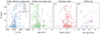 |
Fig. 1 Orbital obliquity distributions of those transiting exoplanets with values determined from the Rossiter-McLaughlin anomaly. (a)Distribution of λ with the temperature of the host star, where it is quite evident that giant planets around hot stars are almost entirely on misaligned orbits. (b) Distribution of λ with the scaled semi-major axis, whereby giant planets whose orbital semi-major axes are ≲ 10 R⋆ tend to be on highly misaligned orbits. (c) Same distribution, but for the mass of the planet where the more massive planets present a larger sample of misaligned orbits. (d) Distribution of λ as a function of the estimated stellar age for those targets where an estimation is available (from NASA exoplanet archive September 2021). In all panels HD 332231 b is represented as the purple point. |
2 Observations and data preparation
We observed a single transit of HD 332231 b on the night of 18-10-2020 spanning the entire night and consequently out of transit observations were obtained during the two nights on either side. The observations were performed with the high dispersion échelle spectrograph CARMENES (Quirrenbach et al. 2014) installed at the 3.5 m telescope at the Calar Alto Observatory in southern Spain. The instrument consists of two spectrographs covering the visible (VIS) and the near-infrared (NIR) channels separately. The VIS channel covers the range of 0.52–0.96 μm, with resolving power  ~ 94 600, encompassing 55 spectral orders. The NIR channel covers 0.96–1.71 μm within 28 orders at
  ~ 80 400. The instrument offers two fibres for light injection, where fibre A is placed on the astronomical source and fibre B is typically used for calibration purposes. For our observations we placed fibre B on sky to monitor and possibly correct for atmospheric emission lines, as well as remove any potential lunar light contamination. The observations were performed with 400 s exposure time in the VIS channeland 406 s in the NIR, to account for different detector readout times in the two channels. 43 exposures were taken on the night of 18-10, of which only the last 4 were out of transit, as well as 15 and 14 exposures on the nights before and after, respectively. The on-sky configuration of the observations are shown in panel a of Fig. 2.
2.1 Data reduction
The recorded spectra were subsequently reduced using the caracal reduction pipeline (CARMENES Reduction And Calibration; Caballero et al. 2016), which considers all standard astronomical data reduction steps, including a flat-relative optimal extraction algorithm (Zechmeister et al. 2014). The wavelength calibration is performed using Th-Ne and U-Ne lamps for the VIS andNIR channels, respectively, both in combination with a Fabry-Pérot etalon. The wavelengths were given in the observatory frame and in vacuum. The median S/N values for the in-transit spectra (the night of 18–10) are 98 (~0.74 μm) and 90 (~1.23 μm), for the VIS and NIR channels, respectively. The variations of the S/N values for both channels are presented in panel b of Fig. 2.
2.2 Telluric correction
Stellar spectra obtained with ground-based facilities are always inherently affected by the presence of the Earth’s atmosphere.This telluric impact manifests itself as both absorption and emission features, which significantly depend on the location of the observatory and local meteorological conditions. In particular, the atmospheric humidity and temperature profiles along the line of sight of the observations dictate the specific shapes and depths of those telluric lines, which are highly time-dependent. For our observations the variations of humidity along the line of sight, obtained from the modelling routine presented below, are shown in panel c of Fig. 2.
In this study we present results from the initial set of spectra, as well as those that have been corrected for the telluric absorption features. The emission features, most prominent in the NIR channel, are simply masked out. For the correction of the telluric absorption features we used ESO’s molecfit routines (Kausch et al. 2015; Smette et al. 2015) version 1.5.9, which synthetically model the lines using a line-by-line radiative transfer model. In order to model line shapes and depths, the code requires the atmosphericpressure profile, the initial guess for which it calculates from the humidity and temperature profiles that it obtains from the GDAS2 (Global Data Assimilation System) database. The optimal atmospheric profiles are then obtained through minimisation routines, given the recorded spectra. As molecfit requires one-dimensional spectra, we stitched all the spectral orders from a single exposure together, creating one spectrum for each pair of VIS and NIR observation.
For the fitting algorithm of molecfit, we included the main atmospheric optical and NIR absorbers of O2, H2O, CO2 and CH4, allowed the continuum to be modelled with a local polynomial of the 4th order and relative convergence criterion of 10−10. The line shapes were modelled using a Voigt profile, which is assumed as variable to account for the instrumental profile variation with wavelength. Example regions for all the fitted species are shown in Fig. 3.
In order to remove the telluric absorption signature from the original two-dimensional spectra (échelle order-by-order data matrices), the corrected spectrum obtained from molecfit was resampled on to the wavelength grids of the individual échelle orders and stored as fits files for further analysis.
As an alternative to correcting the telluric absorption with molecfit, we also used the SYSREM algorithm, which is equivalent to a Principal Component Analysis (PCA) algorithm for unequal uncertainties (Tamuz et al. 2005), to remove the pseudo-stationary telluric and stellar absorption lines from the spectral matrices. This approach has been shown in a number of studies to effectively remove the unwanted stellar and Earth atmospheric signals from the recorded spectra (for example Birkby et al. 2013; Sánchez-López et al. 2020). However, we chose not to further explore the SYSREM reduced data, neither for the calculation of RVs nor for the atmospheric search. As SYSREM does not distinguish between thetelluric and stellar lines and removes them both simultaneously, measurements of stellar RVs are therefore not feasible. With regard to the planetary atmospheric search, since HD 332231 b has a relatively small Kp, meaning that any potential planetary atmospheric absorption signal does not shift significantly from one frame to the next, a significant portion of such signal would most likely also be removed by SYSREM along with the stationary stellar and telluric lines.
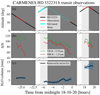 |
Fig. 2 Geometry and conditions for CARMENES observations of HD 332231 b transit. (a) Altitude of the target at the observatory, whereby the red lines present the duration of the observations, with the cyan line representing the full exoplanetary transit. (b) S/N of the spectra calculated by the pipeline in the VIS and NIR channels, at the given specific wavelengths. (c) Retrieved water vapour column density by molecfit in mm, with the 1σ confidence shaded in light blue. In all panels the dark and light shaded regions are the astronomical night and twilight, respectively, whereby thetime axis has been broken for better presentation and midnight is in UT. Please note that no atmospheric seeing values were recorded at the observatory for the observations and the cause of the discrepancy in the S/N values of the first night observations in the VIS and NIR channels is not entirely clear. |
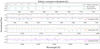 |
Fig. 3 Process of telluric absorption correction of the CARMENES spectra using molecfit. The panels show zooms into regions where the main absorbers are, those being O2, H2O, CO2 and CH4, from top to bottom respectively. The modelled telluric transmission spectrum is presented as a solid black line, shifted vertically for clarity, where the zero flux level is indicated with the dashed line. In the bottom panel some sky emission lines are clearly visible, which are masked at the analysis stage. |
3 Analysis
3.1 RV calculation
We obtained the RV values of the star for the full set of observations using the serval pipeline (Zechmeister et al. 2018), applying it to both sets of raw and telluric corrected spectra from the VIS and NIR channels. This pipeline calculates the RVs through a template matching approach (Butler et al. 1996; Zechmeister et al. 2018), which it constructs by coadding all available spectra for the target. It provides values which are corrected for instrumental drift, as well as secular acceleration. Additionally, the pipeline provides a whole host of spectral diagnostics, some of which are plotted in Fig. 4. Further to the pipeline calculated values, we also measured the RVs by fitting a Gaussian peak to the cross correlation function (CCF; Pepe et al. 2002) of the observed spectra with a phoenix stellar model (Husser et al. 2013) matching best the parameters of HD 332231 and observed no statistically significant differences between the two sets of results (all pairs of values within 1σ). Subsequently, throughout this analysis we present RV results calculated by the pipeline through the template-matching approach. These calculated RV values are presented in Fig. 5, whereby a comparison between the values estimated from the raw and telluric corrected spectra is made. Considering only the out of transit spectra, the RV jitter for the target reduces by ~0.44 m s−1; namely reduced from 8.11 m s−1 for the RVs measured from the raw spectra to 7.67 m s−1 for those estimated from the telluric corrected spectra. The improvements made to stellar RV measurements through telluric correction of high resolution spectra have previously been demonstrated in a number of studies (Artigau et al. 2014; Cunha et al. 2014; Figueira et al. 2016; Kimeswenger et al. 2021). The calculated RV values from both sets of spectra are given in Table A.1. Furthermore, we ignored the RV values determined from the NIR channel, which presented significantly larger uncertainties and jitter as compared to the VIS channel data (cf. Fig. 5). This is rather expected due to the lower S/N spectra in this channel owing to the spectral type of the star, as well as the presence of significant telluric absorption residuals and sky emission lines.
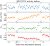 |
Fig. 4 Stellar activity diagnostics calculated by serval. From top to bottom: Ca II IRT index calculated from the middle line of the triplet at ±15 km s−1; the chromatic RV index, which represents the dependence of RV on wavelength and is clearly affected by the transiting planet; Hα activity index calculated for bin a of ±40 km s−1 centred on the line core; and the differential Line Width again impacted by line deformation caused by the transiting planet. Overall the star presents no significant sign of variability due to activity. |
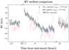 |
Fig. 5 HD 332231 RVs measured during the exoplanet transit, as well as pre- and post-transit epochs. The two VIS sets of measurements are made for the raw pipeline-corrected spectra (blue) and telluric-corrected spectra (black). The raw spectra havebeen shifted along the time axis for clarity. Additionally, the RVs measured from the NIR channel data have also been plotted in the background as red triangles, which have also been shifted along the time axis in the opposite direction. |
3.2 Obliquity measurement
In order to possibly refine the orbital parameters obtained by Dalba et al. (2020), as well as model the RM effect, we defined a composite Keplerian model for a circular orbit of a transiting planet, namely one that also includes the RM effect. We assumed a circular orbit as Dalba et al. (2020) obtained a value for eccentricity consistent with ~0 ( ). This was performed using the modelSuite sub-routine from the PyAstronomy python package (Czesla et al. 2019), which employs the formulation of Ohta et al. (2005) for the analytical description of the RM effect. In order to estimate best fitting values for the free parameters, we ran Markov chain Monte Carlo (MCMC) simulations with 106 steps, burning in the first 105, through which we sampled from the posterior probability distributions. The best fit model, fitted to the three data sets used (HIRES/Keck, APF/Lick (Dalba et al. 2020) and CARMENES), is shown in panel a of Fig. 6, with the phase-foldedRV curve shown in panel b and a zoom into the in-transit region, showing clearly the RM effect and fitted model, in panel c of the same figure. The best fit parameters and their uncertainties, the prior assumptions, as well as a comparison to previously published values are given in Table 1. We note that the last 4 observations performed during the night of 18-10, which are out of transit, present large and significant residuals for the fitted RM model. The nature of this offset is not entirely clear and it is most likely due to the fact that they were taken for the star at very high airmass (1.75→ 1.98). In order to investigate whether these data points bias any of the results for the fitted parameters, we performed the analysis twice; once with all the data included and a second time with these data points masked. The results from fitting data with masked out of transit points are given in Figs. 6 and 7 and their equivalents with all the data points included in Figs. B.1 and B.2. A comparison between the posterior distributions shows that the inclusion of these 4 datapoints only marginally impacts the final outcome and the results are not sensitive to them in any statistically significant way.
For the fitting of the model, we fixed the scaled semi-major axis (a∕R⋆) and the inclination of the planetary orbit (i) to those values found by Dalba et al. (2020) from fitting the TESS transit light curves with an analytical model. This method provides much more stringent solutions as compared to what could be obtained from fitting the RM effect. Furthermore, the inclination of the stellar rotation axis (I⋆) is also fixed to 90 deg, since leaving it as a free parameter did not result in convergence of the posterior. This fact, of course, means that our fitted value for the projected rotational velocity of the star (ν sin I⋆) is only an upper limit. All other parameters were taken as free, with the assumed prior distributions, as well as the best fit values derived from the analysis of posterior probabilities, given in Table 1. These posterior probability distributions are plotted in Fig. 7.
From this analysis we obtained a value of  deg for the orbital obliquity angle (λ) of HD 332231 b, with
 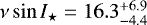 km s−1. The value ofλ has been plotted in the four parameter spaces presented earlier in Fig. 1. The best fit RM model to the in-transit data has been highlighted in panel c of Fig. 6, where 300 random realisations from the inner 1σ posterior distributions have also been drawn, representing the uncertainty in the final fitted model.
We note that there exists a degeneracy between the mid-transit time (T0) and the obliquity angle (λ), as is evidentfrom their mutual posterior plot in Fig. 7. Ideally one would fix the mid-transit time to the value derived from the ephemeris obtained from photometry as that method measures this value with a much higher precision than the RM analysis. However, since there are 24 orbits of the planet around its host star between the epoch given by Dalba et al. (2020) and the one observed for this study, the uncertainty in the predicted mid-transit time in our CARMENES observations are rather large. This uncertainty is approximately taken as the extremes of the uniform prior distribution assumed in our fitting analysis given in Table 1. To assess the impact that this apparent correlation has on the determined obliquity value, we also ran the analysis with the mid-transit time fixed to the one predicted from TESS ephemeris. This approach led to an obliquity value of  deg, indicating that the present degeneracy does not significantly alter the conclusion of moderate misalignment.
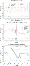 |
Fig. 6 Joint RM+RV analysis of all available RV values for HD 332231, excluding the last 4 out of transit points of CARMENES 18-10 observations shown as red points. (a) Joint analysis of previously obtained RV data from spectrographs at Keck (HIRES) and Lick (APF) observatories (Dalba et al. 2020), together with the data obtained with CARMENES. (b) Same data phase-folded for our derived system parameters from the fit above. (c) Zoom into the epoch of CARMENES observations (including the planetary transit) and the fitted RM function to the data. The thin grey lines are 300 random realisations drawn from 1σ regions of the posteriors. The lime dashed line represents the best fit model when λ is fixed to zero, performed for the purpose of robustness estimation. The residuals of this model are omitted for clarity. |
3.3 Transmission spectroscopy
We searched for possible atmospheric signatures from individually resolved lines emanating from the exoplanet. This is performed through two distinct, albeit fundamentally equivalent, approaches, namely; (1) searching for absorption from strong singular transition lines from species such as Na, K, H or He, or (2) systematically adding absorption signals from a multitude of weaker lines through the cross correlation technique.
The first of the two aforementioned methods has previously been employed in a number of studies to detect a host of atomic species in the upper atmospheres in a multitude of transiting exoplanets. An up to date list of these detected species through narrowband transmission spectroscopy is given in Table C.1. We performed this analysis of HD 332231b for all four of theseneutral species, the results for which are shown in Fig. 8. It is quite evident that the precision at which the data probes the atmosphere is far below what is needed for any possible detection in this atmosphere due to its relatively low equilibrium temperature. Furthermore, a comparison to atmospheric models suggests that placingany upper limits on the temperature or abundances from these data is not particularly informative. These models are calculated with the petitRADTRANS package (Mollière et al. 2019), with equilibrium chemistry considered through FastChem (Stock et al. 2018), examples of which are shown in two panels of Fig. 8.
In addition to this narrow-band approach, we searched for the possible presence of H2O in the atmosphere through the addition of absorption signals from a multitude of individually resolved lines in various strong bands of water in the visible and the near-IR wavelengths. This was performed through the calculation of the CCF of the telluric-corrected spectra in the stellar rest frame with atmospheric templates. The weighted CCF is defined as:
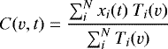 (1)
(1)
where T(ν) is the atmospheric template Doppler shifted to velocity ν, and x(t) is the residual planet spectrum observed at time t. We note that in order to perform the operation in the numerator, both T and x must necessarily be sampled along the same wavelength grid, which is typically achieved by calculating the template at very high resolution and re-sampling it onto the observational wavelength grid. The cross correlation C is subsequently a two-dimensional matrix with rows representing epochs of observations and the columns spanning the velocity space being probed. During this analysis, for a slightly more comprehensive assessment of data quality and detection limits, we calculate a grid of models varying in equilibrium temperature and metallicity and inject them into the residual planet spectra through multiplication. The abundance profiles for this range of models calculated with the equilibrium chemistry code FastChem are presented in Fig. 9.
The cross correlation maps including the injected signals were then systematically summed for a range of planetary radial velocities to obtain the so-called velocity-velocity maps from which detection significances are determined. We performed this analysis for H2O only, takingadvantage of the deep absorption bands in the near-IR wavelengths, as shown in the top panel of Fig. 10. The FastChem equilibrium chemistry model for the calculated planetary Teq, solar C/O and metallicity, for a wide range of species is given in Fig. C.1.
As mentioned above, atmospheric models, calculated using petitRADTRANS and FastChem, spanning in temperature and metallicity were injected into the data and their corresponding peaks in the velocity maps were compared to the variance of the entire map to determine the significance at which each point in the parameter space was detected. A smoothed map of this detection space is shown in the main panel of Fig. 10, where it is evident, given the quality of the data, that for the expected equilibrium temperature of the planet any presence of H2O in the atmosphere would not be detectable. In fact much higher temperatures and abundances are necessary for any potential signal to be accessible. One important caveat that we note with this analysis is that we have assumed a C/O ratio equal to that of the solar value, as well as a cloudless and symmetric atmosphere in hydrostatic and chemical equilibrium. All such assumptions, of course, haveimpacts upon the detectability space to varying degrees.
Orbital and physical parameters of HD 332231 b system from simultaneous RV and RM modelling of all data available, excluding those masked.
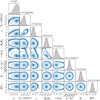 |
Fig. 7 Posterior distributions for the fitted parameters of the RV+RM model. The results are for data where the last 4 data points of CARMENES 18–10 observations have been masked. The median values are quoted as solutions, with the 16th and 84th quartiles given as uncertainties at the top of each column, which are represented as vertical grey dashed lines. All posteriors are modelled well with a Gaussian function with the exception of the mid-transit time, where a double-degenerate solution is derived, as well as λ and ν sin I⋆, where slightly skewed normal distributions are used. In the parameter-parameter plots, 1, 2 and 3σ levels are presented as solid blue lines. |
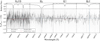 |
Fig. 8 Narrowband transmission spectroscopy of strong transition lines. The upper panels present the composite out of transit stellar spectrum. We note that, with the exception of He I, all the absorption lines present in the stellar spectrum correspond to the species being probed, labelled above each column. The bottom panels present the transmission spectra. The thin grey lines are the individual in-transit residuals shifted to the planetary rest frame. The black lines are the weighted mean of all those shifted residuals. The rest-frame wavelength of each individual transition probed are indicated with vertical blue dashed lines. For Na and K, two atmospheric models of solar metallicity and C/O, with equilibrium temperatures of 876 and 1100 K have been over plotted. |
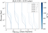 |
Fig. 9 H2O abundance profiles in mass fraction, χ. These are calculated for HD 332231 b, for a range of atmospheric equilibrium temperatures, 825 ≤ Teq ≤ 1100 K and metallicities, − 2 ≤[Fe/H] ≤ 2, with C/O fixed to the solar value of 0.55. These profiles, determined with FastChem, were subsequently used to calculate the models injected into the data, retrieval of which yields the detection space presented in Fig. 10. |
4 Discussion
4.1 Robustness of λ measurement
From the analysis of the RV values measured for HD 332231, we presented a moderately misaligned orbit for the warm sub-Saturn planetary companion of this star. This obliquity angle was measured through the fitting of an RV+RM model to all the available data points, whereby thein-transit data were almost exclusively obtained through our observations with CARMENES. This angle was measured at λ 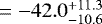 deg, which in thecontext of the relatively small, warm planet sample (presented in panel b of Fig. 1), presents a rather rare moderately misaligned orbit.
In order to assess the significance of this measurement, we performed a statistical comparison between the currently fitted model and one in which λ is fixed to 0 deg. We fitted all the available data again with an identical procedure to the one described in Sect. 3.2, whereby the only difference was that the planetary orbit is assumed to be completely aligned with the stellar rotation axis (λ = 0). The result of this analysis is shown in panel c of Fig. 6, as the lime dashed line. We then compare these two models to the data obtained with CARMENES only (excluding the masked points) to determine the significance of fit improvement by keeping λ free. Making the approximation that the residuals of both models are normally distributed, we calculate the likelihood ratio, LR, as:

where  are the log likelihood values of the models with λ fixed and taken as a free parameter. This ratio corresponds to p = 0.00015, with the critical value at P = 0.005 for the degree of freedom 1 being 7.879. Therefore, we reject the null hypothesis (H0 : no statistically significant difference between the variances of the residuals) at high significance and conclude that the model with free λ describes best the data. The F-ratio, which in this case is a monotone transformation of the likelihood ratio, also results in an identical conclusion.
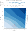 |
Fig. 10 Assessing the quality of CARMENES observations for the potential detection of H2O in the atmosphere of HD 332231 b. Top panel: example of a transmission model calculated with petitRADTRANS (Teq = 876 K and [Fe/H] = 0), normalised to a baseline estimated from the continuum species only and convolved with the instrumental profile. Bottom panel: detection significances for the injected models, smoothed with a Gaussian filter of σ = 1. The expected location of HD 332231 b’s atmosphere for its estimated equilibrium temperature and assumed solar metallicity has been indicated as the red data point. |
4.2 Tidal effects
Albrecht et al. (2012) estimate the realignment time scale for planets with host stars with convective envelopes (τCE) as:
 (2)
(2)
which is estimated through a calibration of relations derived by Zahn (1977), with binary star observations. We chose to use this relation, as opposed to its equivalent for those stars with radiative envelopes, because HD 332231 is a main sequence star with a measured effective temperatureof  K, in other words spectral type F8 with a radiative core and a convective envelope. This time scale for HD 332231 b is therefore estimated as ~ 1016 yr, far exceeding the age of the universe. Subsequently, assuming that the host star has mainly a convective envelope, tidal interactions with the host likely have played a minimal role in altering the obliquity of the planetary orbit.
However, given that the stellar temperature is relatively close to the Kraft break limit (~6200 K; Kraft 1967), where the transition from convective to radiative envelopes is expected, we also considered the realignment time scale for theradiative regime. Zahn (1977) estimate this as:
 (3)
(3)
which for the HD 332231 system is estimated as ~ 1021 yr. Therefore, if the star in fact does have a significant radiative envelope, the tidal effects are expected to be even less significant.
4.3 Misalignment due to a hypothetical external companion
Rice et al. (2021) recently suggested that giant planets around cooler stars, those with convective envelopes and therefore below the Kraft limit, tend to be on more misaligned orbits as compared to those orbiting hotter stars with radiative envelopes. Such trend, if indeed observed for a large sample, could be indicative of mechanisms such as those proposed by Anderson & Lai (2018). They suggest that the obliquity of a giant planet could be excited by an external, modestly inclined companion, due to a secular resonance that occurs when the precession rate of the stellar spin axis is similar to the nodal precession rate of the inner planet.
To investigate such a possibility, we searched for the RV signal of a hypothetical outer companion in the residuals of our model shown in panel a of Fig. 6. We did not however detect any statistically significant signal in the current data, the periodogram for which is shown in Fig. 11. Higher precision RV measurements, with a longer baseline are required to definitively confirm or reject the presence of an outer companion in this system, thereby testing the aforementioned hypothesis.
5 Conclusions
In this study we presented high resolution spectroscopic transit observations of the warm sub-Saturn HD 332231 b, using the CARMENES spectrograph. The correction of the telluric absorption features using molecfit improved the precision of the RV values obtained from those recorded spectra. Measurements of various activity diagnostics indicated that the observations are not likely to be affected by intrinsic variability of the star, which was further corroborated by the stability of the long term photometry of the star obtained by TESS (Dalba et al. 2020).
We measured a projected spin-orbit obliquity angle (λ) of  deg for HD 332231 b, which presents a moderately misaligned planet, with a relatively large orbital period. In the context of planet formation theory presented in Sect. 1, such finding would suggest that those formation theories not invoking planetary migration are favoured. However, for such conclusions to be made concrete, certainly a much larger sample of obliquity measurements for this class of warm transiting planets is required. This is, of course, made rather difficult by the rarity and duration of the transits of those planets. We also discussed the robustness of the measured obliquity value through a statistical model comparison and showed that the inferred measurement significantly improves the residuals of the fitted model, as compared to an aligned orbit. Trivially, it was shown that tidal effects of the host star have not played a role in altering the alignment of the planetary orbital orientation. The residuals of the model were searched for the presence of an outer companion that could possibly excite the obliquity of the inner planet, which resulted in a non-detection.
As an aside, we also analysed the spectra for atmospheric signatures through a couple of distinct methods; namely narrowband transmission spectroscopy of strong, singular transition lines and cross correlation analysis with models containing a myriad of atmospheric lines of H2O. We showed that given the precision of the obtained spectra, it is not feasible to detect any atmospheric characteristics of this planet, especially considering its relatively low estimated equilibrium temperature of 876K. Through an injection and retrieval routine, we presented a slice through the detection parameter space of the atmosphere for a range of metallicities and equilibrium temperatures. In order for such data to be amenable to atmospheric studies, higher precision instrumentation coupled to much larger aperture telescopes are required, a problem which spectrographs such as HIRES at the ELT (Marconi et al. 2021) will address.
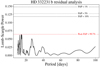 |
Fig. 11 Lomb-Scargle periodogram of the HD 332231 RV residuals for the RV+RM model of the warm-Saturn planet detected from TESS photometry. 1, 5 and 10% False Alarm Probability (FAP) thresholds have been indicated. We do not detect any statistically significant periodic signal in the residuals. The red dashed line shows the FAP for the maximum peak identified in the periodogram. |
Acknowledgements
CARMENES is an instrument at the Centro Astronómico Hispano-Alemán (CAHA) at Calar Alto (Almería, Spain), operated jointly by the Junta de Andalucía and the Instituto de Astrofísica de Andalucía (CSIC). The authors wish to express their sincere thanks to all members of the Calar Alto staff for their expert support of the instrument and telescope operation. We acknowledge financial support from the Agencia Estatal de Investigación of the Ministerio de Ciencia, Innovación y Universidades through projects Ref. PID2019-110689RB-I00/AEI/10.13039/501100011033 and the Centre of Excellence “Severo Ochoa” award to the Instituto de Astrofísica de Andalucía (SEV-2017-0709). We also acknowledge the use of the ExoAtmospheres database during the preparation of this work and thank the team at the IAC for their excellent work preparing such a useful database. E.S. acknowledges support from ANID - Millennium Science Initiative - ICN12_009. K.M. acknowledges support from the Excellence Cluster ORIGINS, which is funded by the Deutsche Forschungsgemeinschaft (DFG, German Research Foundation) under Germany’s Excellence Strategy - EXC-2094 - 390783311. A.S.L. acknowledges funding from the European Research Council under the European Union’s Horizon 2020 research and innovation program under grant agreement No 694513. Beside those explicitly mentioned in the manuscript, throughout this work the following python packages have been used: astropy (Astropy Collaboration 2018), corner (Foreman-Mackey 2016), matplotlib (Hunter 2007), NumPy (Harris et al. 2020), pandas (Pandas development team 2020), PyMC (Salvatier et al. 2016) and SciPy (Virtanen et al. 2020).
Appendix A Calculated RVs
RV values calculated by the serval pipeline from both raw and telluric corrected spectra.
Caracal calculated RVs.
Appendix B Model fit to all data
Here we present the fitted RV+RM model, as well as the posterior distributions, where all the data points are considered. Namely, the four out of transit data points have not been masked.
Appendix C Atmospheric analysis
C.1 Narrowband detections
In Table C.1 we summarise the list of species detected in exoplanetary atmospheres through the method of narrowband transmission spectroscopy, using high resolution échelle spectroscopy.
C.2 FastChem abundances
Here we present the equilibrium chemistry model calculated us- ing the FastChem code, for an atmosphere with solar C/O and metallicity, and Teq equal to that estimated for HD 332231 b, 876 K.
Summary of detected species in exoplanetary atmospheres from the narrowband transmission spectroscopy method.
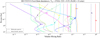 |
Fig. C.1 Equilibrium chemistry model for HD 332231 b calculated with FastChem. The calculations are made for an atmosphere with Teq of 876 K, and solar C/O and metallicity. For clarity the most abundant species are included, with the molecular species plotted as solid lines and those ionic and atomic species plotted with dashed lines. |
References
- Albrecht, S., Winn, J. N., Johnson, J. A., et al. 2012, ApJ, 757, 18 [NASA ADS] [CrossRef] [Google Scholar]
- Allart, R., Bourrier, V., Lovis, C., et al. 2018, Science, 362, 1384 [Google Scholar]
- Allart, R., Bourrier, V., Lovis, C., et al. 2019, A&A, 623, A58 [NASA ADS] [CrossRef] [EDP Sciences] [Google Scholar]
- Alonso-Floriano, F. J., Snellen, I. A. G., Czesla, S., et al. 2019, A&A, 629, A110 [NASA ADS] [CrossRef] [EDP Sciences] [Google Scholar]
- Anderson, K. R., & Lai, D. 2018, MNRAS, 480, 1402 [NASA ADS] [CrossRef] [Google Scholar]
- Anderson, K. R., Winn, J. N., & Penev, K. 2021, ApJ, 914, 56 [NASA ADS] [CrossRef] [Google Scholar]
- Artigau, É., Astudillo-Defru, N., Delfosse, X., et al. 2014, SPIE Conf. Ser., 9149, 914905 [NASA ADS] [Google Scholar]
- Astropy Collaboration, (Price-Whelan, et al. 2018), AJ, 156, 123 [NASA ADS] [CrossRef] [Google Scholar]
- Bate, M. R., Lodato, G., & Pringle, J. E. 2010, MNRAS, 401, 1505 [NASA ADS] [CrossRef] [Google Scholar]
- Batygin, K. 2012, Nature, 491, 418 [NASA ADS] [CrossRef] [Google Scholar]
- Birkby, J. L., de Kok, R. J., Brogi, M., et al. 2013, MNRAS, 436, L35 [Google Scholar]
- Borsa, F., Allart, R., Casasayas-Barris, N., et al. 2021, A&A, 645, A24 [EDP Sciences] [Google Scholar]
- Butler, R. P., Marcy, G. W., Williams, E., et al. 1996, PASP, 108, 500 [Google Scholar]
- Caballero, J. A., Guàrdia, J., López del Fresno, M., et al. 2016, SPIE Conf. Ser., 9910, 99100E [Google Scholar]
- Cabot, S. H. C., Madhusudhan, N., Welbanks, L., Piette, A., & Gandhi, S. 2020, MNRAS, 494, 363 [Google Scholar]
- Casasayas-Barris, N., Palle, E., Nowak, G., et al. 2017, A&A, 608, A135 [NASA ADS] [CrossRef] [EDP Sciences] [Google Scholar]
- Casasayas-Barris, N., Pallé, E., Yan, F., et al. 2018, A&A, 616, A151 [NASA ADS] [CrossRef] [EDP Sciences] [Google Scholar]
- Casasayas-Barris, N., Pallé, E., Yan, F., et al. 2019, A&A, 628, A9 [NASA ADS] [CrossRef] [EDP Sciences] [Google Scholar]
- Cunha, D., Santos, N. C., Figueira, P., et al. 2014, A&A, 568, A35 [NASA ADS] [CrossRef] [EDP Sciences] [Google Scholar]
- Czesla, S., Schröter, S., Schneider, C. P., et al. 2019, PyA: Python astronomy-related packages [Google Scholar]
- Dalba, P. A., Gupta, A. F., Rodriguez, J. E., et al. 2020, AJ, 159, 241 [NASA ADS] [CrossRef] [Google Scholar]
- Dawson, R. I. 2014, ApJ, 790, L31 [NASA ADS] [CrossRef] [Google Scholar]
- Dawson, R. I., & Johnson, J. A. 2018, ARA&A, 56, 175 [Google Scholar]
- de Laplace P. S. 1796, Exposition du système du Monde (New York: Prodinnova) [Google Scholar]
- Dong, S., Katz, B., & Socrates, A. 2014, ApJ, 781, L5 [Google Scholar]
- Figueira, P., Adibekyan, V. Z., Oshagh, M., et al. 2016, A&A, 586, A101 [NASA ADS] [CrossRef] [EDP Sciences] [Google Scholar]
- Foreman-Mackey, D. 2016, J. Open Source Softw., 1, 24 [Google Scholar]
- Gandolfi, D., Hébrard, G., Alonso, R., et al. 2010, A&A, 524, A55 [NASA ADS] [CrossRef] [EDP Sciences] [Google Scholar]
- Gingerich, O. 1973, Proc. Am. Philos. Soc., 117, 513 [Google Scholar]
- Harris, C. R., Millman, K. J., van der Walt, S. J., et al. 2020, Nature, 585, 357 [NASA ADS] [CrossRef] [Google Scholar]
- Hébrard, G., Evans, T. M., Alonso, R., et al. 2011, A&A, 533, A130 [NASA ADS] [CrossRef] [EDP Sciences] [Google Scholar]
- Hoeijmakers, H. J., Ehrenreich, D., Kitzmann, D., et al. 2019, A&A, 627, A165 [NASA ADS] [CrossRef] [EDP Sciences] [Google Scholar]
- Hoeijmakers, H. J., Cabot, S. H. C., Zhao, L., et al. 2020a, A&A, 641, A120 [EDP Sciences] [Google Scholar]
- Hoeijmakers, H. J., Seidel, J. V., Pino, L., et al. 2020b, A&A, 641, A123 [NASA ADS] [CrossRef] [EDP Sciences] [Google Scholar]
- Huber, D., Carter, J. A., Barbieri, M., et al. 2013, Science, 342, 331 [Google Scholar]
- Hunter, J. D. 2007, Comput. Sci. Eng., 9, 90 [NASA ADS] [CrossRef] [Google Scholar]
- Husser, T. O., Wende-von Berg, S., Dreizler, S., et al. 2013, A&A, 553, A6 [NASA ADS] [CrossRef] [EDP Sciences] [Google Scholar]
- Jensen, A. G., Cauley, P. W., Redfield, S., Cochran, W. D., & Endl, M. 2018, AJ, 156, 154 [Google Scholar]
- Katz, B., Dong, S., & Malhotra, R. 2011, Phys. Rev. Lett., 107, 181101 [NASA ADS] [CrossRef] [Google Scholar]
- Kausch, W., Noll, S., Smette, A., et al. 2015, A&A, 576, A78 [NASA ADS] [CrossRef] [EDP Sciences] [Google Scholar]
- Kimeswenger, S., Rainer, M., Przybilla, N., & Kausch, W. 2021, AJ, 161, 66 [NASA ADS] [CrossRef] [Google Scholar]
- Kirk, J., Alam, M. K., López-Morales, M., & Zeng, L. 2020, AJ, 159, 115 [Google Scholar]
- Kraft, R. P. 1967, ApJ, 150, 551 [Google Scholar]
- Kuiper, G. P. 1951, Proc. Natl. Acad. Sci. USA, 37, 1 [NASA ADS] [CrossRef] [Google Scholar]
- Laskar, J., & Robutel, P. 1993, Nature, 361, 608 [Google Scholar]
- Lendl, M., Csizmadia, S., Deline, A., et al. 2020, A&A, 643, A94 [EDP Sciences] [Google Scholar]
- Mancini, L., Esposito, M., Covino, E., et al. 2018, A&A, 613, A41 [NASA ADS] [CrossRef] [EDP Sciences] [Google Scholar]
- Marconi, A., Abreu, M., Adibekyan, V., et al. 2021, The Messenger, 182, 27 [NASA ADS] [Google Scholar]
- Marzari, F. 2014, MNRAS, 444, 1419 [NASA ADS] [CrossRef] [Google Scholar]
- McLaughlin, D. B. 1924, ApJ, 60, 22 [Google Scholar]
- Millholland, S., & Laughlin, G. 2019, Nat. Astron., 3, 424 [Google Scholar]
- Mollière, P., Wardenier, J. P., van Boekel, R., et al. 2019, A&A, 627, A67 [Google Scholar]
- Naoz, S., Farr,W. M., Lithwick, Y., Rasio, F. A., & Teyssandier, J. 2011, Nature, 473, 187 [NASA ADS] [CrossRef] [Google Scholar]
- Nortmann, L., Pallé, E., Salz, M., et al. 2018, Science, 362, 1388 [Google Scholar]
- Ohta, Y., Taruya, A., & Suto, Y. 2005, ApJ, 622, 1118 [Google Scholar]
- Palle, E., Nortmann, L., Casasayas-Barris, N., et al. 2020, A&A, 638, A61 [EDP Sciences] [Google Scholar]
- Pandas development team 2020, pandas-dev/pandas: Pandas [Google Scholar]
- Pepe, F., Mayor, M., Galland, F., et al. 2002, A&A, 388, 632 [NASA ADS] [CrossRef] [EDP Sciences] [Google Scholar]
- Petrovich, C. 2015, ApJ, 805, 75 [NASA ADS] [CrossRef] [Google Scholar]
- Queloz, D., Eggenberger, A., Mayor, M., et al. 2000, A&A, 359, L13 [NASA ADS] [Google Scholar]
- Quirrenbach, A., Amado, P. J., Caballero, J. A., et al. 2014, SPIE Conf. Ser., 9147, 91471F [Google Scholar]
- Rasio, Frederic A., & Ford, Eric B., 1996, Science, 274, 954 [NASA ADS] [CrossRef] [Google Scholar]
- Rice, M., Wang, S., Howard, A. W., et al. 2021, AJ, 162, 182 [NASA ADS] [CrossRef] [Google Scholar]
- Ricker, G. R., Winn, J. N., Vanderspek, R., et al. 2015, J. Astron. Teles. Instrum., Syst., 1, 014003 [Google Scholar]
- Rossiter, R. A. 1924, ApJ, 60, 15 [Google Scholar]
- Safsten, E. D., Dawson, R. I., & Wolfgang, A. 2020, AJ, 160, 214 [NASA ADS] [CrossRef] [Google Scholar]
- Salvatier, J., Wiecki, T. V., & Fonnesbeck, C. 2016, PeerJ Comput. Sci., 2, e55 [Google Scholar]
- Salz, M., Czesla, S., Schneider, P. C., et al. 2018, A&A, 620, A97 [NASA ADS] [CrossRef] [EDP Sciences] [Google Scholar]
- Sánchez-López, A., López-Puertas, M., Snellen, I. A. G., et al. 2020, A&A, 643, A24 [NASA ADS] [CrossRef] [EDP Sciences] [Google Scholar]
- Sedaghati, E., MacDonald, R. J., Casasayas-Barris, N., et al. 2021, MNRAS, 505, 435 [NASA ADS] [CrossRef] [Google Scholar]
- Seidel, J. V., Ehrenreich, D., Wyttenbach, A., et al. 2019, A&A, 623, A166 [NASA ADS] [CrossRef] [EDP Sciences] [Google Scholar]
- Seidel, J. V., Ehrenreich, D., Bourrier, V., et al. 2020, A&A, 641, L7 [NASA ADS] [CrossRef] [EDP Sciences] [Google Scholar]
- Smette, A., Sana, H., Noll, S., et al. 2015, A&A, 576, A77 [NASA ADS] [CrossRef] [EDP Sciences] [Google Scholar]
- Souami, D., & Souchay, J. 2012, A&A, 543, A133 [NASA ADS] [CrossRef] [EDP Sciences] [Google Scholar]
- Southworth, J. 2011, MNRAS, 417, 2166 [Google Scholar]
- Spake, J. J., Oklopčić, A., & Hillenbrand, L. A. 2021, AJ, 162, 284 [NASA ADS] [CrossRef] [Google Scholar]
- Stock, J. W., Kitzmann, D., Patzer, A. B. C., & Sedlmayr, E. 2018, MNRAS, 479, 865 [NASA ADS] [Google Scholar]
- Storch, N. I., & Lai, D. 2014, MNRAS, 438, 1526 [CrossRef] [Google Scholar]
- Tabernero, H. M., Zapatero Osorio, M. R., Allart, R., et al. 2021, A&A, 646, A158 [NASA ADS] [CrossRef] [EDP Sciences] [Google Scholar]
- Tamuz, O., Mazeh, T., & Zucker, S. 2005, MNRAS, 356, 1466 [Google Scholar]
- Triaud, A. H. M. J. 2011, A&A, 534, L6 [NASA ADS] [CrossRef] [EDP Sciences] [Google Scholar]
- Triaud, A. H. M. J. 2018, Handbook of Exoplanets, The Rossiter-McLaughlin Effect in Exoplanet Research, eds. H. J. Deeg, & J. A. Belmonte (Berlin: Springer), 2 [Google Scholar]
- Triaud, A. H. M. J., Queloz, D., Bouchy, F., et al. 2009, A&A, 506, 377 [NASA ADS] [CrossRef] [EDP Sciences] [Google Scholar]
- Virtanen, P., Gommers, R., Oliphant, T. E., et al. 2020, Nat. Methods, 17, 261 [Google Scholar]
- Winn, J. N., Noyes, R. W., Holman, M. J., et al. 2005, ApJ, 631, 1215 [Google Scholar]
- Winn, J. N., Johnson, J. A., Marcy, G. W., et al. 2006, ApJ, 653, L69 [NASA ADS] [CrossRef] [Google Scholar]
- Winn, J. N., Johnson, J. A., Albrecht, S., et al. 2009, ApJ, 703, L99 [NASA ADS] [CrossRef] [Google Scholar]
- Winn, J. N., Fabrycky, D., Albrecht, S., & Johnson, J. A. 2010, ApJ, 718, L145 [Google Scholar]
- Wyttenbach, A., Lovis, C., Ehrenreich, D., et al. 2017, A&A, 602, A36 [NASA ADS] [CrossRef] [EDP Sciences] [Google Scholar]
- Wyttenbach, A., Mollière, P., Ehrenreich, D., et al. 2020, A&A, 638, A87 [EDP Sciences] [Google Scholar]
- Yan, F., Wyttenbach, A., Casasayas-Barris, N., et al. 2021, A&A, 645, A22 [EDP Sciences] [Google Scholar]
- Yu, L., Zhou, G., Rodriguez, J. E., et al. 2018, AJ, 156, 250 [NASA ADS] [CrossRef] [Google Scholar]
- Zahn, J. P. 1977, A&A, 500, 121 [NASA ADS] [Google Scholar]
- Zechmeister, M., Anglada-Escudé, G., & Reiners, A. 2014, A&A, 561, A59 [NASA ADS] [CrossRef] [EDP Sciences] [Google Scholar]
- Zechmeister, M., Reiners, A., Amado, P. J., et al. 2018, A&A, 609, A12 [NASA ADS] [CrossRef] [EDP Sciences] [Google Scholar]
All Tables
Orbital and physical parameters of HD 332231 b system from simultaneous RV and RM modelling of all data available, excluding those masked.
Summary of detected species in exoplanetary atmospheres from the narrowband transmission spectroscopy method.
All Figures
|
Fig. 1 Orbital obliquity distributions of those transiting exoplanets with values determined from the Rossiter-McLaughlin anomaly. (a)Distribution of λ with the temperature of the host star, where it is quite evident that giant planets around hot stars are almost entirely on misaligned orbits. (b) Distribution of λ with the scaled semi-major axis, whereby giant planets whose orbital semi-major axes are ≲ 10 R⋆ tend to be on highly misaligned orbits. (c) Same distribution, but for the mass of the planet where the more massive planets present a larger sample of misaligned orbits. (d) Distribution of λ as a function of the estimated stellar age for those targets where an estimation is available (from NASA exoplanet archive September 2021). In all panels HD 332231 b is represented as the purple point. |
| In the text | |
|
Fig. 2 Geometry and conditions for CARMENES observations of HD 332231 b transit. (a) Altitude of the target at the observatory, whereby the red lines present the duration of the observations, with the cyan line representing the full exoplanetary transit. (b) S/N of the spectra calculated by the pipeline in the VIS and NIR channels, at the given specific wavelengths. (c) Retrieved water vapour column density by molecfit in mm, with the 1σ confidence shaded in light blue. In all panels the dark and light shaded regions are the astronomical night and twilight, respectively, whereby thetime axis has been broken for better presentation and midnight is in UT. Please note that no atmospheric seeing values were recorded at the observatory for the observations and the cause of the discrepancy in the S/N values of the first night observations in the VIS and NIR channels is not entirely clear. |
| In the text | |
|
Fig. 3 Process of telluric absorption correction of the CARMENES spectra using molecfit. The panels show zooms into regions where the main absorbers are, those being O2, H2O, CO2 and CH4, from top to bottom respectively. The modelled telluric transmission spectrum is presented as a solid black line, shifted vertically for clarity, where the zero flux level is indicated with the dashed line. In the bottom panel some sky emission lines are clearly visible, which are masked at the analysis stage. |
| In the text | |
|
Fig. 4 Stellar activity diagnostics calculated by serval. From top to bottom: Ca II IRT index calculated from the middle line of the triplet at ±15 km s−1; the chromatic RV index, which represents the dependence of RV on wavelength and is clearly affected by the transiting planet; Hα activity index calculated for bin a of ±40 km s−1 centred on the line core; and the differential Line Width again impacted by line deformation caused by the transiting planet. Overall the star presents no significant sign of variability due to activity. |
| In the text | |
|
Fig. 5 HD 332231 RVs measured during the exoplanet transit, as well as pre- and post-transit epochs. The two VIS sets of measurements are made for the raw pipeline-corrected spectra (blue) and telluric-corrected spectra (black). The raw spectra havebeen shifted along the time axis for clarity. Additionally, the RVs measured from the NIR channel data have also been plotted in the background as red triangles, which have also been shifted along the time axis in the opposite direction. |
| In the text | |
|
Fig. 6 Joint RM+RV analysis of all available RV values for HD 332231, excluding the last 4 out of transit points of CARMENES 18-10 observations shown as red points. (a) Joint analysis of previously obtained RV data from spectrographs at Keck (HIRES) and Lick (APF) observatories (Dalba et al. 2020), together with the data obtained with CARMENES. (b) Same data phase-folded for our derived system parameters from the fit above. (c) Zoom into the epoch of CARMENES observations (including the planetary transit) and the fitted RM function to the data. The thin grey lines are 300 random realisations drawn from 1σ regions of the posteriors. The lime dashed line represents the best fit model when λ is fixed to zero, performed for the purpose of robustness estimation. The residuals of this model are omitted for clarity. |
| In the text | |
|
Fig. 7 Posterior distributions for the fitted parameters of the RV+RM model. The results are for data where the last 4 data points of CARMENES 18–10 observations have been masked. The median values are quoted as solutions, with the 16th and 84th quartiles given as uncertainties at the top of each column, which are represented as vertical grey dashed lines. All posteriors are modelled well with a Gaussian function with the exception of the mid-transit time, where a double-degenerate solution is derived, as well as λ and ν sin I⋆, where slightly skewed normal distributions are used. In the parameter-parameter plots, 1, 2 and 3σ levels are presented as solid blue lines. |
| In the text | |
|
Fig. 8 Narrowband transmission spectroscopy of strong transition lines. The upper panels present the composite out of transit stellar spectrum. We note that, with the exception of He I, all the absorption lines present in the stellar spectrum correspond to the species being probed, labelled above each column. The bottom panels present the transmission spectra. The thin grey lines are the individual in-transit residuals shifted to the planetary rest frame. The black lines are the weighted mean of all those shifted residuals. The rest-frame wavelength of each individual transition probed are indicated with vertical blue dashed lines. For Na and K, two atmospheric models of solar metallicity and C/O, with equilibrium temperatures of 876 and 1100 K have been over plotted. |
| In the text | |
|
Fig. 9 H2O abundance profiles in mass fraction, χ. These are calculated for HD 332231 b, for a range of atmospheric equilibrium temperatures, 825 ≤ Teq ≤ 1100 K and metallicities, − 2 ≤[Fe/H] ≤ 2, with C/O fixed to the solar value of 0.55. These profiles, determined with FastChem, were subsequently used to calculate the models injected into the data, retrieval of which yields the detection space presented in Fig. 10. |
| In the text | |
|
Fig. 10 Assessing the quality of CARMENES observations for the potential detection of H2O in the atmosphere of HD 332231 b. Top panel: example of a transmission model calculated with petitRADTRANS (Teq = 876 K and [Fe/H] = 0), normalised to a baseline estimated from the continuum species only and convolved with the instrumental profile. Bottom panel: detection significances for the injected models, smoothed with a Gaussian filter of σ = 1. The expected location of HD 332231 b’s atmosphere for its estimated equilibrium temperature and assumed solar metallicity has been indicated as the red data point. |
| In the text | |
|
Fig. 11 Lomb-Scargle periodogram of the HD 332231 RV residuals for the RV+RM model of the warm-Saturn planet detected from TESS photometry. 1, 5 and 10% False Alarm Probability (FAP) thresholds have been indicated. We do not detect any statistically significant periodic signal in the residuals. The red dashed line shows the FAP for the maximum peak identified in the periodogram. |
| In the text | |
 |
Fig. B.1 Same as Fig. 6, but with all the data points considered. |
| In the text | |
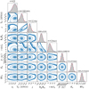 |
Fig. B.2 Same as Fig. 7, but for the fitting routine where all the data points are considered. |
| In the text | |
|
Fig. C.1 Equilibrium chemistry model for HD 332231 b calculated with FastChem. The calculations are made for an atmosphere with Teq of 876 K, and solar C/O and metallicity. For clarity the most abundant species are included, with the molecular species plotted as solid lines and those ionic and atomic species plotted with dashed lines. |
| In the text | |
Current usage metrics show cumulative count of Article Views (full-text article views including HTML views, PDF and ePub downloads, according to the available data) and Abstracts Views on Vision4Press platform.
Data correspond to usage on the plateform after 2015. The current usage metrics is available 48-96 hours after online publication and is updated daily on week days.
Initial download of the metrics may take a while.