| Issue |
A&A
Volume 659, March 2022
|
|
|---|---|---|
| Article Number | A92 | |
| Number of page(s) | 24 | |
| Section | Extragalactic astronomy | |
| DOI | https://doi.org/10.1051/0004-6361/202141901 | |
| Published online | 10 March 2022 | |
Galaxy populations in the Hydra I cluster from the VEGAS survey
I. Optical properties of a large sample of dwarf galaxies⋆
1
INAF – Astronomical Observatory of Capodimonte, Salita Moiariello 16, 80131 Naples, Italy
e-mail: This email address is being protected from spambots. You need JavaScript enabled to view it.
2
University of Naples “Federico II”, C.U. Monte Sant’Angelo, Via Cinthia, 80126 Naples, Italy
3
Kapteyn Institute, University of Groningen, Landleven 12, 9747 AD Groningen, The Netherlands
4
Space Physics and Astronomy Research Unit, University of Oulu, PO Box 3000 90014 Oulu, Finland
5
Centre for Astrophysics & Supercomputing, Swinburne University of Technology, Hawthorn, VIC 3122, Australia
6
INAF Osservatorio Astronomico d’Abruzzo, Via Maggini, 64100 Teramo, Italy
7
European Southern Observatory, Karl-Schwarzschild-Strasse 2, 85748 Garching bei München, Germany
8
Instituto de Astrofísica, Facultad de Física, Pontificia Universidad Católica de Chile, Av. Vicuña Mackenna 4860, 7820436 Macul, Santiago, Chile
9
INAF – Astronomical Observatory of Rome, Via Frascati, 33, 00078 Monte Porzio Catone, Rome, Italy
10
INAF – Astronomical Observatory of Padova, Via dell’Osservatorio 8, 36012 Asiago, VI, Italy
11
Department of Physics, University of Oxford, Denys Wilkinson Building, Keble Road, Oxford OX1 3RH, UK
12
European Southern Observatory, Alonso de Cordova 3107, Vitacura, Santiago, Chile
Received:
29
July
2021
Accepted:
8
December
2021
Abstract
Context. Due to their relatively low stellar mass content and diffuse nature, the evolution of dwarf galaxies can be strongly affected by their environment. Analyzing the properties of the dwarf galaxies over a wide range of luminosities, sizes, morphological types, and environments, we can obtain insights about their evolution. At ∼50 Mpc, the Hydra I cluster of galaxies is among the closest cluster in the z ≃ 0 Universe, and an ideal environment to study dwarf galaxy properties in a cluster environment.
Aims. We exploit deep imaging data of the Hydra I cluster to construct a new photometric catalog of dwarf galaxies in the cluster core, which is then used to derive properties of the Hydra I cluster dwarf galaxy population as well as to compare it with other clusters. Moreover, we investigate the dependency of dwarf galaxy properties on their surrounding environment.
Methods. The new wide-field g- and r-band images of the Hydra I cluster obtained with the OmegaCAM camera on the VLT Survey Telescope (VST) in the context of the VST Early-type GAlaxy Survey (VEGAS) were used to study the dwarf galaxy population in the Hydra I cluster core down to r-band magnitude Mr = −11.5 mag. We used an automatic detection tool to identify dwarf galaxies from a ∼1 deg2 field centered on the Hydra I core, covering almost half of the cluster virial radius. The photometric pipeline was used to estimate the principal photometric parameters for all targets. Scaling relations and visual inspection were used to assess the cluster membership and construct a new dwarf galaxy catalog. Finally, based on the new catalog, we studied the structural (Sérsic index n, effective radius Re, and axis ratio) and photometric (colors and surface brightness) properties of the dwarf galaxies, also investigating how they vary as a function of clustercentric distance.
Results. The new Hydra I dwarf catalog contains 317 galaxies with a luminosity between −18.5 < Mr < −11.5 mag, a semi-major axis larger than ∼200 pc (a = 0.84″), of which 202 are new detections, and previously unknown dwarf galaxies in the Hydra I central region. We estimate that our detection efficiency reaches 50% at the limiting magnitude Mr = −11.5 mag, and at the mean effective surface brightness μ̄e,r = 26.5 mag arcsec−2. We present the standard scaling relations for dwarf galaxies, which are color-magnitude, size-luminosity, and Sérsic n-magnitude relations, and compare them with other nearby clusters. We find that there are no observational differences for dwarfs scaling relations in clusters of different sizes. We study the spatial distribution of galaxies, finding evidence for the presence of substructures within half the virial radius. We also find that mid- and high-luminosity dwarfs (Mr < −14.5 mag) become, on average, redder toward the cluster center, and that they have a mild increase in Re with increasing clustercentric distance, similar to what is observed for the Fornax cluster. No clear clustercentric trends are reported for surface brightness and Sérsic index. Considering galaxies in the same magnitude bins, we find that for high and mid-luminosity dwarfs (Mr < −13.5 mag), the g − r color is redder for the brighter surface brightness and higher Sérsic n index objects. This finding is consistent with the effects of harassment and/or partial gas stripping.
Key words: galaxies: dwarf / galaxies: evolution / galaxies: clusters: individual: Hydra I (Abell 1060) / galaxies: photometry
Catalogue (full Table C.1) is only available at the CDS via anonymous ftp to cdsarc.u-strasbg.fr (130.79.128.5) or via http://cdsarc.u-strasbg.fr/viz-bin/cat/J/A+A/659/A92
© ESO 2022
1. Introduction
Dwarf galaxies are the most abundant type of galaxies in the Universe, and they play a crucial role in testing the current Λ cold dark matter cosmological model (ΛCDM; Bullock & Boylan-Kolchin 2017), and galaxy formation and evolution theories. Indeed, dwarf-sized proto-galactic fragments built up the bulges of massive galaxies very rapidly, which are their building blocks, while other (metal-poor) dwarf galaxies were accreted later to form the outer galactic halos (growth through bottom-up assembly processes Springel et al. 2005; Mancillas et al. 2019). Dwarfs are an important resource to study the physics of galaxies because they have a low stellar mass and, they are usually diffuse and, therefore, are more affected by environmental processes. Furthermore, dwarfs are found both in isolation, in groups of galaxies, and in dense, cluster environments. Different samples can be used to investigate intrinsic (internal) processes versus extrinsic (environmental) processes that shape their evolution. Some of the relatively recent examples of low density environment studies are Leaman et al. (2014), Gallart et al. (2015), Kacharov et al. (2017), Hermosa Muñoz et al. (2020), and in cluster environment: Sánchez-Janssen et al. (2008), Peng et al. (2010a, 2012, 2014) investigated processes shaping dwarf galaxies in cluster environments. Hence, in conclusion, the combination of their abundance and their vulnerability makes them a suitable instrument to investigate the effects of environment on galaxy evolution.
Recent deep, wide-field surveys provided homogeneous and complete samples of galaxy populations, down to the low luminosity regime. Among these, the Next Generation Virgo cluster Survey (NGVS; Ferrarese et al. 2012), the Next Generation Fornax Survey (NGFS; Muñoz et al. 2015; Eigenthaler et al. 2018), the VST Early-type GAlaxy Survey (VEGAS; Capaccioli et al. 2015; Iodice et al. 2021), the Fornax Deep Survey (FDS; Peletier et al. 2020), and the Mass Assembly of early Type gaLAxies with their fine Structures (MATLAS; Duc et al. 2015; Habas et al. 2020) revealed large samples of faint galaxies in various environments, which were previously unknown, constituting a powerful resource to analyze how galaxies change as a function of different environments. On the theoretical side, the current large-scale cosmological simulations (such as IllustrisTNG, Pillepich et al. 2018) have reached sufficient high resolution, making a direct comparison with dwarf galaxies with a stellar mass of 108 − 9 M⊙ now possible. However, this stellar mass range is typical of larger dwarf galaxies, and simulations are still not good at reproducing galaxies below that stellar mass limit (for example, look at the EAGLE simulation lower mass limit, Schaye et al. 2015).
The faintest galaxies discovered in the new imaging surveys usually lack accurate distance information, and many of them have such a low surface brightness that obtaining spectroscopic redshifts for a complete sample is not possible with the available instruments. Thus, to assess the cluster memberships of very faint objects, one needs to exploit their photometric properties. Surface brightness fluctuations (SBFs) enable us to determine the distance of a galaxy measuring the variance in its light distribution, arising from fluctuations in the numbers of and luminosities of individual stars per resolution element (Tonry & Schneider 1988). However, measuring SBFs for large samples of faint galaxies at distances D > 20 Mpc is really challenging with observing facilities (see Mieske et al. 2003, 2005; Carlsten et al. 2019; Greco et al. 2021; Blakeslee & Cantiello 2018, to get an idea of the potential of the SBFs method, and its application to the Hydra I cluster). Another way is to use the photometric redshifts, often used to obtain distances for a large samples of galaxies (see for example Bilicki et al. 2018). Finally, it is possible to address cluster memberships using the known scaling relations for galaxies. In fact, in clusters there are up to thousands of galaxies located at a similar distance, and many of their properties scale with each other. On the other hand, background galaxies are spread over a wide range of distances, so their apparent parameters do not follow any relation. Useful relations commonly used for identifying cluster members are the color-magnitude and the magnitude-surface brightness relations (see for instance Misgeld et al. 2009). Already the work by Binggeli et al. (1985) have used colors, the luminosity-surface brightness relation and galaxy morphology to define the membership status in the Virgo cluster. More recently, Venhola et al. (2018, 2019) used the mentioned scaling relations to construct the FDS dwarf galaxy catalog for the Fornax cluster.
Correlations among global parameters of galaxies are not only useful to assess their membership, but they also provide insight into the physical processes that impact the formation and evolution mechanisms of these galaxies. For example, luminosity, color, size, surface brightness, light concentration, central velocity dispersion are related to each other, (such as Visvanathan & Sandage 1977; Kormendy 1977; Faber & Jackson 1976; Djorgovski & Davis 1987) Specifically, the fundamental plane, the color-magnitude relation (CMR) and the luminosity-surface brightness relation link the physical properties of the underlying stellar populations and the global structural properties with the galaxy mass. Investigating these scaling relations in multiple environments sets constraints for galaxy evolutionary models. Interestingly, since the observed properties of galaxies reflect their evolution, it is possible to infer how they reached the actual configuration, and what were the main processes responsible for their evolution. The evolutionary processes can be divided into two main categories: internal and environmental. The set of the former processes is usually called mass quenching because they are all related to the mass of the galaxy. These internal mechanisms usually affect mostly massive early-type galaxies (Su et al. 2021). Studies focused on isolated early-type galaxies, for which external influences can be excluded, have shown that mass quenching is effective only for galaxies more massive than 109 M⊙ (Geha et al. 2012). Concerning dense environments, such as galaxy clusters, dwarf galaxies can experience various environmental processes. Ram-pressure stripping is a process affecting the interstellar matter in galaxies: when a galaxy falls into a cluster, its cold gas component interacts with the hot gas of the cluster, and the pressure between the two gas components removes the cold gas from the galaxy’s potential well (Gunn & Gott 1972). Because the stars are not removed, galaxy evolution after the gas-removal happens via fading of its stellar populations (id est, through internal processes). If not all the gas of the galaxy is removed at once, it is likely that a small gas fraction is retained in the center of the potential well, where it may have become overpressurized leading to star formation. Indeed, there are dwarf galaxies in clusters with blue centers, which are indicative of a recent star formation episode (for example Lisker et al. 2006; Hamraz et al. 2019). These cases are often referred to as partial ram-pressure stripping. In dense environments, cluster galaxies go through high speed encounters, and the cumulative effect of multiple high-speed collisions is the stripping of stellar, gas and dark matter components from galaxies, the material of which will build up the intra-cluster component. This process is called harassment (Moore et al. 1996, 1998). Harassment is not efficient in removing a large number of stars (Smith et al. 2015), and generally the material is stripped off firstly from galaxy’s outskirts, increasing its light concentration. Moreover, the star formation activity is quenched (Moore et al. 1998; Mastropietro et al. 2005). Another drastic consequence of the gravitational interactions is that they can be so strong in the cluster center that they may cause complete disruption of dwarf galaxies (McGlynn 1990; Koch et al. 2012; Sasaki et al. 2007). The ripped off material then ends up in the intra-cluster medium, in which it piles up.
On this paper we focus on the cluster core, where vivid examples of tidal dissolution of galaxies have already been observed (Arnaboldi et al. 2012; Koch et al. 2012). However, observationally there is still a lack of systematic studies analyzing the environmental effects, and the properties of dwarf galaxies for a wide portion of the Hydra I cluster. Recently, the FDS approached this problem from an observational point of view for the Fornax cluster dwarf galaxies, using imaging data from the ESO VLT Survey Telescope (Venhola et al. 2019), and so we aim to analyze Hydra I cluster similarly in this paper, with images from the same instrument.
Hydra I, also known as Abell 1060, is among the closest and largest galaxy clusters in the nearby Universe. It is the prototype of an evolved and dynamically relaxed cluster, dominated by early-type galaxies and having a regular core shape. The cluster center is inhabited by its two brightest members, NGC 3309 and NGC 3311, of which the latter is the central Dominant (cD) galaxy of the cluster. Both are surrounded by an extended diffuse stellar halo (Arnaboldi et al. 2012).
In Table 1 we summarize the adopted values for the different parameters of Hydra I. Throughout the paper we assume the average cluster distance of 51 ± 4 Mpc ((m − M) = 33.55 mag), assuming  1. Richter et al. (1982) and Richter (1987) found evidence for an empty space of 40 − 50 Mpc extending in front and behind the Hydra I cluster along the line of sight. This implies that background objects appear smaller on the images than Hydra I galaxies (at least a factor ×0.5), and that the cluster is relatively isolated in redshift space.
Hydra I galaxy cluster properties.
The center of the cluster-wide X-ray emission looks to be centered near NGC 3311 (slightly displaced toward northwest Hayakawa et al. 2004). The total mass estimated from X-rays measurements is relatively high compared to the number of known galaxies in the cluster (Tamura et al. 2000; Loewenstein & Mushotzky 1996). This could mean either that the fraction of dark matter (DM) content in Hydra I is somehow higher than seen in similar clusters, or that there is a number of still undetected faint galaxies. The work of Misgeld et al. (2008), as well as the spectroscopic catalog by Christlein & Zabludoff (2003) show a rich environment, with a large population of dwarf galaxies in its core. However, the first work is focused on a small area around the cluster core, while the latter is limited to mid-luminosity dwarfs (MR ≲ −14 mag).
Several other works, studying the light distribution and the kinematics of the Hydra I cluster core, demonstrated that the mass assembly is still active around NGC 3311, and showed the presence of ongoing interactions between galaxies (Arnaboldi et al. 2012; Ventimiglia et al. 2011; Hilker et al. 2018; Barbosa et al. 2018, 2021; Koch et al. 2012). Hereafter, we assume that the cluster center is represented by NGC 3311: RA = 159.17842 deg, and Dec = −27.528339 deg (respectively 10:36:42.82 and −27:31:42.02).
In this paper we present a new catalog of dwarf galaxy (Mr > −18.5 mag) members of Hydra I galaxy cluster. The aim of the work is to use this new catalog to study the structural (effective radius Re, Sérsic index n, and axis ratio) and photometrical (colors, surface brightness) properties of the galaxies, as well as the differences between the populations of galaxies of different morphological types in the Hydra I cluster. In Sect. 2 we describe the observations used in this work; then we explain all the steps necessary to construct the Hydra cluster dwarf catalog in Sects. 3 and 4. The final catalog of dwarf galaxies is presented in Sect. 5. In Sect. 6 we present the dwarfs spatial distribution, their colors, their structural scaling relations, and how these properties vary as a function of the clustercentric distance and of their total luminosity. Finally, in Sects. 7 and 8 we discuss and summarize the results.
2. Deep images of the Hydra I cluster from VEGAS
The Hydra I galaxy cluster is one of the targets of the VEGAS research project. VEGAS is a deep multiband (u, g, r, i) imaging survey (Capaccioli et al. 2015; Iodice et al. 2020a, 2021), carried out at the European Southern Observatory (ESO) VLT Survey Telescope (VST, Schipani et al. 2012). The optical camera OmegaCAM (Kuijken 2011) on the VST, used to record wide field images spanning 1 × 1 deg2 field of view, has a mosaic of 32 CCDs with a resolution of 0.21 arcsec pix−1.
The deep g and r bands images of the Hydra I cluster have been already presented in Iodice et al. (2020b). The observations have been acquired with the step-dither observing strategy, which guarantees an accurate estimate of the sky background (see for instance Iodice et al. 2016; Venhola et al. 2018). The data reduction has been performed using VST-Tube, one of the dedicated pipelines to process OmegaCAM images (Grado et al. 2012; Capaccioli et al. 2015). The sky field has been acquired on the west side of the cluster, adopting an overlap of ∼0.3 deg with the 1 deg field centered on the core of the cluster. Therefore, the final sky-subtracted reduced mosaic for the Hydra I cluster extends over 1° ×2°, corresponding to ∼0.9 × 1.8 Mpc at Hydra’s distance, which means that the cluster is symmetrically covered out to ≈0.4 virial radius. During the data acquisition, we have taken special care to put the bright (7th-magnitude) foreground star, which is on the NE side of the cluster core, always in one of the two wide OmegaCam gaps, thereby reducing the scattered light. The residual light from this bright star has been modeled and subtracted from the mosaic, in both bands. The light distribution of the second brightest star in the field, located SE the core, is also modeled and subtracted from the parent image (see Fig. 1 in Iodice et al. 2020b).
Thanks to the long integration times (2.8 h in the g-band and 3.22 h in the r-band), and the specific observing strategy, the final stacked images reach surface brightness depths of μg = 28.6 ± 0.2 mag arcsec−2, and μr = 28.1 ± 0.2 mag arcsec−2. They are derived as the flux corresponding to 5σ, with σ averaged over 1 arcsec2 from an empty area. The median FWHM of the point spread function are 0.81″ in the r-band, and 0.85″ in the g-band.
In this work we focus on a 56.7 × 46.6 arcmin2 wide portion of the VST/OmegaCAM mosaic that maps a symmetric area around the cluster core (Fig. 1). This portion, at the assumed Hydra I’s distance, corresponds to ∼0.8 × 0.7 Mpc, enabling us to study the cluster in a systematic way up to a considerable fraction of the virial radius (≈0.4 Rvir).
 |
Fig. 1. Color composite image (g and r bands) of the VST mosaic’s portion used in this paper (56.7 × 46.6 arcmin2). The two cD galaxies NGC 3311 and NGC 3309, which lie in the cluster center, are labeled in the figure. Close to them, to the left is marked NGC 3312, a large spiral galaxy. Residual light from the two subtracted stars is still visible. North is up, and east is on the left. The color RGB image is created using the Lupton et al. (2004) scheme, using the r-band image as R filter input, the g-band as B filter input, and the average image between r and g bands as G filter input. |
3. Extraction of the sample
In this section we describe the detection algorithm for the Low Surface Brightness (LSB) galaxies, which is based on the method presented in Venhola et al. (2018) and successfully applied to the VST data of the FDS.
3.1. Detection of the sources
We used the automatic detection algorithm SEXTRACTOR (Bertin & Arnouts 1996) to identify dwarf and LSB galaxies in the Hydra I cluster. SEXTRACTOR works detecting objects with a certain number of connected pixels, brighter than a chosen threshold. Hence, the first parameters to configure are the detection threshold and the minimum number of pixels above that value, DETECT_TRESH and DETECT_MINAREA respectively. Both parameters have to be set according to the type of galaxy one wants to detect.
The software creates a background model by defining a grid of image pixels, and then estimating the background level in each grid box. The background grid size is therefore another critical parameters of SEXTRACTOR. For the more extended galaxies the grid size should be set to be large enough to prevent false detections. For the smaller galaxies, which often are spatially blended with brighter ones, the grid size should be set to a smaller value, so that the larger galaxies can be included into the background model.
Following Venhola et al. (2018), we use different parameters for three different classes of objects: Large, LSB, Small sources. We ran SEXTRACTOR in the so-called double-image mode, using the r-band image (after subtracting the light from the two brightest stars) for the detection, while the g-band was used for measurements only. The final combination of the main detection parameters is shown in Table 2.
Main configuration parameters used in SEXTRACTOR for the three different classes of sources.
Given the goal of this work, we focused only on the Small and LSB tables, which both consist of a huge number of sources, over 30 000 and 150 000 objects, respectively. SEXTRACTOR gives as output object lists with a certain number of parameters associated with each detection. Most of these detections are foreground stars, globular clusters hosted by Hydra I galaxies, false detections or unresolved background galaxies, which must be removed from the list. To this aim, we proceeded as follows: firstly, we removed sources with magnitude mr = 99.0 mag or mg = 99.0 mag, which are clearly software errors; secondly, we removed all the objects which contain the SEXTRACTOR flag ≥42; thirdly, we divided the sample into “stars” and “not-stars” using a criterion based on the FLUX RADIUS3. Stars are likely to have smaller flux radii since they are point sources, while galaxies are much less concentrated objects. In a flux radius vs magnitude plot (Fig. 2) this is particularly visible, with stars inhabiting a tight sequence around 1″. This band merges with diffuse objects for magnitude fainter than ∼22 mag. Given that, we have marked all objects with flux radius lower than 0.9″, brighter than mr = 22 mag, as “stars”, and therefore excluded them from the catalogs. We used the same criteria also for the g-band. Finally, we excluded the unresolved galaxies and globular clusters. This is done by removing all the objects with semi-major axis smaller than 4 pixels (or 0.84 arcsec), as measured by SEXTRACTOR’s parameter A_IMAGE, see Fig. 3. This size limit corresponds to ∼200 pc at Hydra’s distance, therefore we are aware that we are excluding also some intrinsically small, unresolved Hydra I cluster galaxies, like for example the smallest Ultra Compact Dwarfs (UCDs, e.g. Misgeld et al. 2011). Importantly, we are not removing from the sample of Hydra I cluster galaxies similar to the Local Group dwarf spheroids (dSphs), that usually have effective radii between 200 pc < Re < 1000 pc.
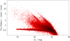 |
Fig. 2. Flux radius in arcsec vs. r-band magnitude. A tight band extends horizontally from mr ∼ 14 mag to ∼22 mag, and it is inhabited by stars. Extended objects are arranged in a more diffuse way. |
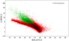 |
Fig. 3. Size-magnitude diagram for detected sources, with size in pixels. Green dots represents the galaxies selected for the final clean catalog, i.e. have semi-major axis larger than 4 pixels, and have passed all the previous steps. |
These selection criteria exclude ∼98% of the initial SEXTRACTOR’s detections in the field. The remaining objects in the two lists were joined, avoiding to insert duplicates: objects within 2 arcsec from each other are considered the same galaxy. For duplicates, parameters and coordinates were taken from the Small list. As a result, a cleaned catalog in all bands is obtained, containing 4535 candidate galaxies for Hydra I. Coordinates, magnitudes and morphological parameters from SEXTRACTOR are used as initial guesses for the photometric pipeline (see next section). We did not filter any further since, as described in the next Section, we use more robust photometric measurements, in order to divide background galaxies from cluster members.
3.2. Efficiency of the detection
In order to determine the typical detection limits, we test the completeness of our detection algorithm. We use a python script to generate iteratively 3000 mock galaxies, divided in bunches of 250 individuals, and added them to 12 template images, that have the same size and seeing conditions of the r-band images. We use the seeing of the r-band because the detection is done on this filter. We also include 30 000 foreground stars to better resemble the observed field4. To simulate the light profiles of artificial galaxies, we use 2D-Sérsic profiles as artificial galaxies, convolved with the PSF of OmegaCAM. Moreover, poissonian noise is added into each pixel. The galaxies are embedded into the template images with random locations and position angles. We chose a wide range of input parameters to cover the expected parameter space of dwarf galaxies and UDGs in the Hydra I cluster, which are summarized in the following:
-
 mag arcsec−2
 -
Re = 0.4 − 8 arcsec (∼0.1 − 2 kpc)
-
Sérsic n = 0.5 − 3.0
-
Axis ratio b/a = 0.2 − 1.0
The only shortcoming of this procedure is that we are not considering galaxies with 2 or more components. However, since LSB galaxies usually do not show many features, this should not affect the detection (Su et al. 2021).
We run SEXTRACTOR on the simulated images, with the same combination of configuration parameters used for science frames. We look at how many objects it is able to identify. For each mock galaxy we require the center to be detected within 2.5 arcsec from the true central coordinates. To understand the effect of the minimum size cut carried out, we remove the objects with A_IMAGES < 0.84 arcsec from the detections. Figure 4 shows how the detection efficiency changes as function of different structural parameters, with and without the minimum size limit. We find that the detection efficiency slightly depends on the Sérsic index so that more peaked galaxies are more efficiently detected. More extended sources are more easily recognized, while there is no clear dependence on the axis ratio, as expected.
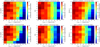 |
Fig. 4. Detection efficiency (number of detected galaxies over number of generated ones in the same bin) of our detection algorithm is shown color-coded such that red means more efficient, while blue less efficient. The efficiency is plotted for effective radius (Re, the pixel scale is 0.21 arcsec pix−1), axis ratio (b/a), and Sérsic index n, as function of mean effective surface brightness, without (top row) and with (bottom row) minimum size limit. The white lines show the 50% detection efficiency limit. |
The detection efficiency reaches 50% at a r-band magnitude value of mr = 23.0 mag and at mean effective surface brightness value of  mag arcsec−2. When the size cut is applied, the 50% efficiency is reached at mr = 22.0 mag and
  mag arcsec−2. We take FDS data for comparison: there, the exposure times in g- and r-band, in a single field, were of 2.3 h, with typical seeing of 1.1 and 1.0 arcsec, and surface brightness depths of 28.4 and 27.8 mag arcsec−2, respectively (Iodice et al. 2016; Venhola et al. 2018). Data used in this work are deeper, and our detection efficiency reaches the 50% level slightly deeper than in FDS. Indeed, Venhola et al. (2018) detection has the limiting r-band magnitude with 50% detection efficiency of mr = 21 mag and
  mag arcsec−2. However, since Fornax has less than half the distance of Hydra I, their dwarf catalog goes fainter than ours by 1 mag (up to mr ≃ −10.5 mag).
3.3. Photometric measurements
In order to identify Hydra I cluster members and to study their optical properties, we derive the photometric parameters for all galaxies in the catalog of candidates as obtained in Sect. 3.1, namely all galaxies that have SEXTRACTOR semi-major axis larger than 0.84 arcsec (∼200 pc). They are derived by fitting the 2D light distributions of all targets using GALFIT (Peng et al. 2002, 2010b), assuming a Sérsic profile to obtain the effective radii (Re), magnitudes and colors, axis ratios and position angles, and Sérsic indices.
To this aim, we run a semi-automatic photometric pipeline over all objects in the final candidates catalog. The pipeline was originally developed to work with VST data of the FDS (Peletier et al. 2020) data, therefore we do not need to modify it. A full description of how the photometric pipeline works is given by Venhola et al. (2017, 2018). Here we briefly list the main operations:
– Post-stamp images of the galaxies are made in both bands, using as center the coordinates of the object as detected by SEXTRACTOR. The semi-width of images is limited to 10 A_IMAGE, again, as measured by SEXTRACTOR. These semi-major axis lengths are not always accurate, and sometimes the cutouts can be too small for the selected galaxy candidates. In such cases we increase the size manually.
– For the stamps of each candidate, other objects than the main galaxy are masked, like faint stars or nearby galaxies. This is done with an automatic masking routine5, followed by a manual masking when needed. When two galaxies are overlapping or are so close that masking is not feasible, both are modeled simultaneously by GALFIT.
– The estimate of the initial input parameters of GALFIT is done by making an azimuthally averaged radial profile of the galaxy, using two pixels wide circular bins. Then the clipped average of each bin is taken to make a cumulative profile up to three times the semi-major axis value (where the semi-major axis is taken from SEXTRACTOR). From the growth curve, effective radius and magnitude values are estimated, and used as input parameters for GALFIT. Also the center is measured at this step: if the object has a clear center, a 2D-parabola is fitted and the peak is considered the center of the galaxy. For galaxies with flat center, SEXTRACTOR’s coordinates are used as center.
– At this point the post stamps are ready for the GALFIT run. The objects are fitted in both g and r band with a single Sérsic function, or with a combination of a Sérsic function and a point-source for the nucleus, if required (it is up to the user to choose, based on the visual appearance of the galaxy). The pipeline allows the Sérsic component to have a different center than the nucleus, because it is possible to have off-centered nuclei6.
– The fits are inspected to see if they resemble real galaxies. The inspection is done by looking at the radial profile with the model overlapped, at the residuals, and the original image with an aperture of radius 1 Re overlaid. The latter is done in order to understand if the estimated Re is reasonable.
The colors of the galaxies are derived separately, the g − r colors are calculated from the g and r band magnitudes within the effective aperture, as calculated from GALFIT models. In particular, we measure the flux in the elliptical effective aperture and calculate the corresponding magnitude. For this task, we use r-band parameters also for g-band measurement, in order to obtain consistent magnitudes. Colors calculated in this way are more stable than using total magnitudes, because in the outermost part of the galaxies the determination of the background can severely affect the colors.
In conclusion, the pipeline returns a catalog containing photometric and structural parameters of the galaxies: the effective radius Re, axis ratio b/a, position angle θ, Sérsic index n, magnitudes and aperture g − r color7. It is important to highlight that we consider only the structural parameters in the r-band, because of the higher S/N.
Inferring accurate errors for the GALFIT models is crucial. As pointed out by Häussler et al. (2007), GALFIT tends to underestimate errors on the fitted parameters. Full details of how we infer errors for the photometric parameters are given in Appendix A.
4. Selection of the cluster galaxies
From the source catalog we aim at distinguishing between the cluster and the background galaxies. The most recent and complete spectroscopic sample for the Hydra I cluster is given by Christlein & Zabludoff (2003), which fully covers the area studied in this work. They consider Hydra I’s member galaxies with recession velocity within the range 2292 − 5723 km s−1. However, the spectroscopic redshift sample of Christlein & Zabludoff (2003) is limited to bright galaxies, therefore calibrated selection limits should be carefully extended to low luminosity.
We exploit the effects of greater distance on galaxy properties to remove background galaxies from our sample. Firstly, with the increasing distance, galaxies appear to have smaller angular sizes, while their surface brightness stays (almost8) constant. Hence intrinsically bright galaxies at large distance will show a low apparent total magnitude, but high surface brightness. On the other hand, cluster galaxies follow the surface brightness vs luminosity relation (Binggeli et al. 1984), thus the fainter the galaxy, the lower the surface brightness. Therefore, we can use this relationship to separate background and foreground galaxies. Galaxies in clusters follow also a color-magnitude relation (CMR), that is they become bluer going to lower luminosities (Visvanathan & Sandage 1977; Roediger et al. 2017; Venhola et al. 2019).
Additionally, large background galaxies can have structures, such as spiral arms or bars, while their angular size is comparable to the size of Hydra I’s dwarfs. These features are unlikely shown by small dwarf galaxies (Janz et al. 2014), although they can be present in the brightest dwarfs. The latter, anyway, are bright enough to have measured spectroscopic redshifts. Hence, there is no degeneracy in that sense, and a visual classification based on galaxies morphological appearance is helpful to further distinguish background galaxies from cluster members.
Optical photometry alone is not sufficient for defining the cluster membership, and some degree of degeneracy exists in the apparent structural and color properties of the cluster galaxies and those at higher redshift. However, calibrating the selection limits using available archival spectroscopic redshifts, it is possible to minimize the degeneracy problem. As shown for example by Venhola et al. (2018), this approach gives satisfying results when supported with a visual classification.
In the following paragraphs we explain in detail the adopted procedure to isolate the Hydra I galaxies in our sample.
4.1. Photometric selection criteria
We proceed in the following order with the selection cuts based on photometry: initially we perform an upper color cut, secondly a cut based on the surface brightness vs luminosity relation, and finally we use a CMR from a previous work on Hydra I (Misgeld et al. 2008). For the upper color cut, we consider the two brightest cluster members, NGC 3311 and NGC 3309, which have g − r color ≃0.8, as reported by Misgeld et al. (2008). Given that limit, we exclude all the galaxies that are at least 0.15 mag redder than the 0.8 mag, that is g − r > 0.95 mag. In Fig. 5 there is an illustration of the color selection we apply here.
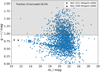 |
Fig. 5. Color selection criteria used to separate the cluster members from the background galaxies. The horizontal dotted line represents the upper color limit we applied, g − r = 0.95 mag: galaxies in the shaded gray area are excluded. The two BCGs are marked with black triangles. |
Doing so, we are mostly ruling out the large background early-type galaxies (ETGs) and spirals, as their intrinsic color could be similar to the largest cluster members, but their apparent color is significantly redder due to the higher redshift. Price et al. (2009) demonstrated that is possible to find in galaxy clusters compact dwarf galaxies that are significantly redder than the sequence defined by normal cluster members. However, usually these systems are at most only marginally redder than the brightest cluster galaxies (Hamraz et al. 2019). We are therefore confident that our limits are sufficiently broad that none of the likely cluster members is excluded. However, some background spirals with a small or no bulge will be still left in the sample.
As second criterion we use the surface brightness vs. magnitude relation. We take confirmed cluster members (Christlein & Zabludoff 2003) and make a linear fit of the  relation. As mentioned by Binggeli et al. (1984), the slope of this relationship appears to flatten for brighter galaxies. Our study is focused on the dwarf population, therefore we fit only the galaxies fainter than mr = 13 mag (corresponding to Mr = −20.5 mag). We then take two standard deviations as confidence level, and exclude all the galaxies that passed the first cut with a
  2σ brighter than the cluster sequence. The left panel of Fig. 6 shows the effect of this selection. With this selection criterion, 17 galaxies from the sample are removed.
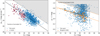 |
Fig. 6. Scaling relations used for the galaxy selection. Left panel: mean effective surface brightness vs total magnitude (r-band) plane for catalog objects that passed the first selection cut. The black solid line is the linear fit of the redshift confirmed cluster members. The data of Christlein & Zabludoff (2003) are represented by red open circles. The dotted line indicates 2 standard deviations from the cluster sequence: the objects in the shaded gray area are removed from the sample. Right panel: color-magnitude diagram for galaxies that passed the first two cuts. Orange triangles are early-type galaxies found by Misgeld et al. (2008), and the orange solid line is their CMR. The dashed line is the 2 rms level we use to define galaxies as members of the Hydra I cluster. |
To further improve the selection, we use the CMR for the early-type dwarf galaxy population of the Hydra I cluster, provided by Eq. (1) in Misgeld et al. (2008). To be sure not to exclude cluster members, we consider an upper confidence interval of 0.24 mag, which is 2 times larger than the root mean square error the authors reported, and remove all galaxies 0.24 mag redder than this sequence. This prevents removing galaxies which are already confirmed cluster members: all dwarf galaxies from Misgeld et al. (2008) sample are included, as shown in the right panel of Fig. 6. We note that even with this cut, the red compact dwarfs are retained within our sample, because g − r ∼ 0.8 mag for mr ≤ 24 mag.
Even after the last cut, the sample of selected galaxies still includes some of the spectroscopically confirmed background galaxies from Christlein & Zabludoff (2003). Considering a tolerance of 5 arcsec for the position of the galaxies, we excluded 69 more galaxies from the sample.
4.2. Visual classification
As a next step, a visual inspection is performed for all galaxies in the selected sample, in order to make morphological classification of each of them. This step is only used to identify more background galaxies and clean the Hydra I sample in this way. It is not used for detailed morphological analysis, and no new galaxy is added at this stage.
To visual classify galaxies, in practice we need extended objects to be sharp and well resolved, thus we decided to exclude all the galaxies with an effective radius smaller than 1 arcsec. This is motivated by considering that the average seeing of the data is 0.8 arcsec. Taking into account that we reach the 50% completeness at mr = 22.0 mag, we limit this analysis to all objects brighter than this limit. The objects that satisfy these two constraints are visual classified, looking at their color and residual images. We divided the galaxies into the following four groups according to their morphology:
-
Late-type: Galaxies that have blue color and have blue star-forming clumps. In this category spirals, blue compact dwarfs and irregular galaxies are included.
-
Early-type with structure: Red galaxies with no blue star-forming clumps, but with structures such as a bar, spiral arms, or a bulge. In this group we include S0s galaxies and dEs with an evident disk component.
-
Smooth early-type: Galaxies that appear red and smooth, with no clear structures. The dwarf ellipticals, and the giant ETGs without structures are included here. We do not distinguish between nucleated and non-nucleated dwarfs; both are added to this group.
-
Background galaxies: Small galaxies that show features like spiral arms or bars. These properties are not likely to appear in low-mass dwarfs (Janz et al. 2014; Su et al. 2021), thus we conclude that they are background galaxies. We are aware that some massive dwarf galaxies can show prominent disk-like features, with star forming regions, resembling spiral galaxies (Lisker et al. 2006; Michea et al. 2021). However, the fraction of light in the disk, compared to the smooth spherical component is low and there is no risk to confuse these dwarfs with the background spirals.
In Fig. 7 we show some examples of galaxies for each morphological category, as we classified them. In total 916 identified galaxies were clear enough to be classified. 569 of them were classified as background systems. The remaining 347 are likely cluster galaxies. Specifically, 288 galaxies were marked as “Smooth early-type galaxies”, 36 as “Late-type galaxies”, and the remaining 23 as “Early-type galaxies with structures”.
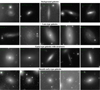 |
Fig. 7. r-band images of the galaxies as they are classified in the visual inspection phase. Green bars are of equal length in each cutout, 10 arcsec. Background galaxies show spiral features, but they are considerably smaller than the Late-type galaxies that inhabit the cluster. The difference between the LTGs and the ETGs with structures in our classification scheme is mainly given by the color, hence is not evident in gray-scale images. |
5. Final catalog and comparison with previous Hydra I catalogs
The final sample of Hydra I cluster members consists of 347 galaxies. We adopt a limit of Mr ≥ −18.5 mag to define our sample of Hydra I dwarf galaxies, which gives a sample of 317. In Table C.1 we present an extract of the complete catalog containing photometric and structural parameters of dwarfs. The catalog covers the Hydra I cluster core, up to 0.4 virial radius, and has a minimum semi-major axis limit of 0.84 arcsec. It reaches a 50% completeness level at the mean effective surface brightness (r-band) value of  mag arcsec−2, and at r-band magnitude Mr = −11.5 mag. 70 galaxies in our sample are spectroscopically confirmed members: we matched our sample with Christlein & Zabludoff (2003) catalog for Hydra I, considering a range of 5 arcsec. Of the 317 galaxies, 61 have already been presented by Misgeld et al. (2008) (in this case considering a tolerance of 3 arcsec on the position). Hence, in this paper we report the discovery of 202 dwarf galaxies, previously unknown, in the central region of Hydra I.
From the sample of Christlein & Zabludoff (2003) we miss 20 galaxies, of which 8 are in the area of the residual light of the two saturated stars, 7 overlap with large galaxies, or bright stars, so that they cannot be distinguished, 1 is on the edge of our image, and only the remaining 4 are the ones we truly missed. It is important to point out that none of these 4 missing galaxies have been excluded during the selection cuts phase.
The Hydra I cluster catalog (HCC) presented in Misgeld et al. (2008) consists of 111 galaxies, down to the magnitude limit of MV ≃ −10 mag. The catalog covers an L-shaped area, made of seven 7′×7′ fields over the cluster core. Their imaging data were obtained with VLT/FORS1, in Johnson V and I filters, with seeing conditions better than ours, averaging between 0.5 and 0.7 arcsec. Matching our sample with the Misgeld et al. (2008) catalog, and considering our magnitude range (−18.5 mag ≤ Mr ≤ −11.5 mag), we miss 30 galaxies. In Table 3 we show their median photometric parameters. These systems are quite faint and small. As shown in Fig. 6, our photometric selection cuts are not excluding any dwarf galaxy from Misgeld et al. (2008). Rather, given their faint nature, we miss them during the detection phase. Misgeld et al. (2008) detection strategy is a combination of visual inspection of the images and the use of SEXTRACTOR detection routines.
Median values of the principal photometric parameters for the 30 missed objects from the Misgeld et al. (2008) Hydra I catalog.
In conclusion, our catalog extends by almost a factor 3 the sample of known Hydra I galaxies within its 0.4 virial radius, making it a more complete tool to exploit the photometric properties of dwarf galaxies in this environment.
6. Results
In this section we present the analysis carried out on the new photometric catalog of dwarf galaxies in the Hydra I cluster. We exploit all the derived photometrical measurements, studying the spatial distribution of the galaxies and deriving several scaling relations, with the final goal of fully characterize the dwarf galaxy population over the central area of the Hydra I cluster. In the following subsections we focus on the main properties derived for the dwarf galaxies in this sample. They represent ∼88% of the galaxy population9 in the studied area of the cluster.
6.1. Spatial distribution of dwarfs and giants
In Fig. 8 we show the locations of the dwarf galaxies in our sample. As expected, the galaxies are strongly concentrated around the center of the Hydra I cluster, dominated by the cD galaxy NGC 3311. The densest region is located within the cluster core (black circle of radius rc = 170 h−1 kpc Girardi et al. 1995). Moreover, even considering the empty area due to the presence of the two heavily saturated stars, which have prevented the detection of some of the faint sources there, the galaxy distribution seems to be approximately symmetric around the two BCGs.
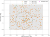 |
Fig. 8. Spatial distribution of the likely Hydra I cluster dwarfs in our sample (orange circles), and giant galaxies from Christlein & Zabludoff (2003), green triangles. The dividing magnitude is at Mr = −18.5 mag. The black circle indicates the cluster core radius rc = 170 h−1 kpc (Girardi et al. 1995), assuming h = 0.72, and the gray area indicates our studied field. The two BCGs, NGC 3311 and NGC 3309 are marked separately as black triangles. The two magenta stars show the position of the two major saturated stars that we masked. In the figure north is up and east is left. |
We derive a smoothed density map of the galaxies, by convolving the galaxy distribution with a Gaussian kernel with a standard deviation of σ = 10′. This is shown in Fig. 9, where also X-ray isophotes are plotted10. From the smoothed distribution we find a pronounced over-density in the northwest of the cluster center. In this region, also the X-ray contours are a bit more broadened, just outside the core radius, and a structure on the southeast of the cluster center. The smoothed distribution also shows that overall, the western side of the cluster is less populated than the eastern side.
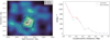 |
Fig. 9. Projected galaxy density distribution inside the Hydra I cluster. Left panel: smoothed number density distribution of the galaxies in the Hydra I galaxy cluster. The observed galaxy distribution is convolved with a Gaussian kernel with σ = 10′. The colored contours highlight the iso-density curves (red, yellow and purple). X-ray contours (thin black lines) are also overlaid to the map. The two giant galaxies at the center of the cluster are represented by the two black triangles, while the magenta stars are the two modeled stars in the field. North is up, east is left. Right panel: projected galaxy surface density, as number of galaxies per square Mpc, plotted against the projected clustercentric distance. Red solid line is the density profile accounting for the area of the two saturated stars, while blue dashed line is the profile without correcting for that area. |
To better understand how the projected galaxy density changes going outward from the cluster center, we derive the radial clustercentric surface density for the dwarf galaxies in our sample. We count the number of galaxies in circular bins, with a step of 4′ in radius (≃60 kpc), and then divide that number by the bin area to get the surface density of the galaxies. We assume a fixed distance for all the cluster members, equal to the distance of the cluster. We plot the projected surface density as function of the clustercentric distance in the right panel of Fig. 9. The plot shows the number density both accounting for the incompleteness in the areas of the two brightest stars, and without correcting for it. We point out that this is the projected surface density, and that we have considered a fix projected clustercentric distance. Therefore a realistic volume density of galaxies could give substantially different results. As expected, on average, a decreasing galaxy density is found with increasing clustercentric distance. The curve is also consistent with the 2D smoothed distribution of galaxies in Fig. 9, as we find some over-densities, instead of a monotonic decreasing profile. A first overdensity at d ∼ 0.2 Mpc corresponds to the southeast group of galaxies, while the second peak at ∼0.35 Mpc traces the north group.
In addition, we compare the spatial distribution of giants and dwarfs, by studying their cumulative distribution as a function of their clustercentric distance, see Fig. 10. We analyze the statistical differences between the two populations using a Kolmogorov–Smirnov (KS) test (Hodges 1958). The p-value of the KS test gives the probability that giant and dwarf galaxies are taken from the same radial distribution, and this resulted to be 0.006. This means that giant and dwarf radial distributions are statistically different. Specifically, Fig. 10 highlights that giant galaxies are more concentrated toward the center of the cluster, with respect to the dwarfs.
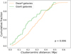 |
Fig. 10. Cumulative functions of the clustercentric distances of giants (Christlein & Zabludoff 2003), green solid line, and of dwarfs, orange dashed line. The label refers to the p-value from the Kolmogorov–Smirnov test. The KS-test result states that the two radial distributions are statistically different. |
6.2. Color-magnitude relation
In Fig. 11 we show the color-magnitude relation (CMR) of the dwarf galaxies in our sample, from Mr = −18.5 mag, down to Mr ≃ −11.5 mag. A well-defined CMR exists for early-type dwarf galaxies in our sample brighter than Mr ≃ −14 mag: on average the brighter the galaxy, the redder its color is. Fainter than that a wide scatter emerges, and nothing clear can be said. We carry out a linear fit to all dwarf data points that were visually classified as ETGs, namely the early-type with structure, and Smooth early-type categories. We obtain:
 (1)
(1)
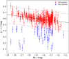 |
Fig. 11. Color-magnitude relation for all Hydra I dwarf galaxies in our catalog. The solid line is the linear fit of the red sequence (Eq. (1)), while the dotted lines are the 2σ deviations from the fit. The two galaxy populations: blue triangles form the blue dwarf population, while red dots are the red dwarfs, with their color errors. |
with a rms of 0.07. The fitted red sequence (RS) is overlaid in the color-magnitude diagram (CMD, Fig. 11). Except for two galaxies, all dwarfs are not redder than 2σ from the fitted RS. As expected, the scatter becomes larger going to fainter magnitudes.
In order to separate late-type from early-type galaxies in a more reliable way than the visual classification, we use the fitted RS to split the dwarf sample into two subpopulations. We refer to the dwarfs which are at least 2σ = 0.14 mag bluer than the RS as blue dwarfs. The remaining objects are named as red dwarfs. A visual representation of this splitting is given in Fig. 11, where we color-code the objects according to this classification scheme. The blue population consists of 43 dwarf galaxies (≃14%), while the red one of 274 dwarfs. Blue dwarfs all have colors g − r < 0.5 mag, and do not follow a clear trend as the ETGs do along the RS, rather they are spread in the bottom part of the CMD. We also notice that there are no blue dwarf galaxies in the range between Mr ∼ −16.5 mag and Mr ∼ −15 mag. In the next sections we analyze other scaling relations between photometric parameters, considering separately the two different dwarf populations.
6.3. Scaling relations for structural parameters
In Fig. 12 we plot the structural parameters ( ) measured for all the dwarf galaxies in our catalog, as function of their total r-band magnitude. Both blue and red galaxy parameters show correlations with Mr. These are highlighted by the running mean trends, shown in the right panels.
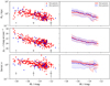 |
Fig. 12. From the top to the bottom row: effective radius Re, mean effective surface brightness in r-band |

Within the errors, in all diagrams the distribution of red and blue dwarfs are very similar, especially up to Mr = −16 mag. At brightest magnitudes, where also errors are smaller, there are more appreciable differences, although they are statistically relevant only for the effective radii. Indeed, the red dwarf galaxies show a flattening in the Re vs. Mr relation toward the bright end (Mr < −16 mag), while blue dwarfs do not. Both size and surface brightness clearly depend on total magnitude, and we see an almost linear correlation. Sérsic index seems to depend too, but given the larger errors it is less clear to confirm. This parameter describes the shape of the galaxy’s radial light profile, where n = 1 represents an exponential profile, whereas larger values indicates more concentrated profiles, and values smaller than 1 represent a flatter profile. The red dwarfs show, on average, a mild increase in the Sérsic index from n ≲ 1 to n ≃ 2, in the range from Mr ≃ −14 mag to Mr ≃ −18 mag, which means that the brighter the red galaxies become, the more centrally concentrated they are. For blue dwarfs it is hard to tell if there is the same trend, given the wide scatter. However, brightest blue dwarf galaxies have on average smaller n than red dwarfs of comparable luminosity. A similar log(n) vs. Mr trend has also been found in other clusters (Misgeld et al. 2009; Venhola et al. 2019, for the Centaurus and Fornax clusters, respectively). Carlsten et al. (2021) also found a correlation between the Sérsic index and the stellar mass of early-type dwarfs, analyzing dwarf satellites around Milky Way like hosts within Local Volume loose groups (D < 12 Mpc). A more detailed comparison is reported in Sect. 7.3.
6.4. Axis ratio
In Fig. 13 (top panel) we show the cumulative distribution of the axis ratio, b/a, for both dwarf populations. The blue distribution grows steeper than the red population for low b/a values, then flattens at b/a ∼ 0.4, and then continues to grow toward unity, reaching it faster than the red galaxies distribution. We compare blue and red dwarf axis ratios performing a KS test between the two cumulative distributions. The p-value is equal to 0.03, indicating that the two distributions are not taken from the same parent distribution (see Sect. 6.1).
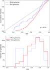 |
Fig. 13. Axis ratio distributions for the red and blue galaxies, represented by the red solid line, and by the blue dashed line, respectively. Top panel: cumulative distributions of the two populations. The black diagonal line shows a flat b/a distribution. The reported value is the p-value of the performed KS test. Bottom panel: fraction of red and blue dwarfs in b/a = 0.1 wide bins. |
Bottom panel of Fig. 13 shows the histogram distributions of the two populations. Both red and blue distributions peak at about b/a = 0.8. A considerable fraction of blue dwarfs (∼30%) have axis ratio between 0.2 and 0.4, while there are few red galaxies with axis ratio lower than 0.4. This is qualitatively consistent with the idea that the early-type galaxies are rounder compared to the late-types, which show more disky features, and therefore prefer lower axis-ratios. However, one has to take into account the fact that we observe a 2D projection of the intrinsic 3D shape distribution of the galaxies, but statistically the 2D observed distribution should reflect a behavior that is linked to the intrinsic 3D shape.
The b/a distribution of dwarf galaxies in the Fornax cluster (Venhola et al. 2019), also considering the separation between late-types and early-types, has the same trend found for the dwarf galaxies in our Hydra I sample. The distribution of non-nucleated dEs in Fornax is very close to the axis-ratio distribution of the red galaxies in Hydra I; indeed the respective cumulative distributions grow with the same rate. Fornax LTGs have qualitatively the same trend of Hydra I blue dwarfs, with a second peak in the distribution between 0.2 and 0.4.
6.5. Clustercentric properties
In order to understand how the environment affects the dwarf galaxies, we analyze how their properties vary depending on their location in the Hydra I cluster. If the role played by the environment is important, we expect to see galaxies with similar luminosity having different properties according to their projected clustercentric distance. However it is important to remind that distances are projected, and hence galaxies might be located further out. We binned the dwarf sample into 2 mag wide magnitude bins. The faintest bin (that is Mr > −12.5 mag) covers a smaller magnitude range, due to our detection limit. Therefore, to make a statistical robust analysis, and a fair comparison with literature, we focus on the first 3 bins. Figure 14 shows the structural parameters as a function of the clustercentric distance for both galaxy populations, divided into the three magnitude bins. To quantitatively test the correlations between the different parameters and the clustercentric distance we use the Spearman’s rank correlation test11, showing the correlation coefficients ρ in each panel of Fig. 14. The correlation coefficients are obtained considering both the whole dwarf population (blue + red), and only the red dwarfs. We find that some parameters behave similarly with respect to the clustercentric distance in all luminosity bins, while some others have different trends for the high luminosity galaxies. More in detail:
-
Red dwarfs become redder moving inward in the bright (−18.5, −16.5 mag) bin, and show the same trend also in the mid-luminosity bin (−16.5, −14.5 mag), but with a weaker correlation. For red dwarfs in the faintest bin, a rather flat trend is observed. Blue dwarfs show the opposite trend, which means they become bluer at larger distances. The trend is much weaker in the intermediate luminosity bin.
-
On average, the effective radius increases with increasing clustercentric distance for red dwarfs in high- and mid-luminosity bins. However, the correlation is weak, and galaxies show a wide scatter. By contrast, both blue and red dwarfs in the range (−14.5, −12.5 mag) show no correlation with distance, and an even wider scatter.
-
A rather flat trend is observed for the mean effective surface brightness
 in each luminosity bin. Only red dwarfs in the mid-magnitude bin exhibit a weak negative correlation, i.e.
  becomes fainter going outward from the center. The opposite weak trend is reported for blue dwarfs in the same bin.
 -
Dwarfs in each magnitude bin do not show any clear trend between the Sérsic index and clustercentric distance. Only bright red dwarfs (Mr < −16.5 mag) have on average slightly increasing n toward the center, with a mild correlation.
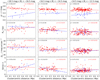 |
Fig. 14. Structural parameters of Hydra’s dwarf galaxies as a function of their projected clustercentric distance. Panel rows from top to bottom show: g − r color, effective radius Re, mean effective surface brightness |

In addition, we study how the two dwarf populations are spatially distributed, producing a clustercentric cumulative distribution, which is shown in Fig. 15. We perform a two-sided KS test to assess the validity of the null hypothesis, namely whether the two samples are drawn from the same distribution. The corresponding p-value is 0.074, or 7.4%. Interestingly, we do not find blue dwarf galaxies, according to our definition, closer than ∼0.15 deg to the cluster center. This is in agreement with the fact that galaxies located at small clustercentric distances have on average entered the cluster earlier, and have already been quenched, explaining the lack of blue dwarfs in the very central region. The red dwarf galaxy distribution grows regularly and approaches unity smoothly.
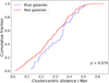 |
Fig. 15. Cumulative clustercentric distributions for both red and blue dwarfs, represented by a red solid line and a blue dashed line, respectively. The number on the bottom is the p-value of the performed KS test. |
7. Discussion
In this paper we present a new catalog of dwarf galaxies in the Hydra I cluster, that more than doubles the previously known samples, based on VEGAS deep imaging data that cover the cluster out to 0.4 Rvir. In the following sections we discuss the two main outcomes of this work: the 2D projected distribution of the galaxies in the cluster and the clustercentric properties of the dwarf galaxy population. Moreover, we extend the comparison of Hydra’s dwarf galaxies properties with the dwarf populations inhabiting other clusters.
7.1. Dwarfs versus Giants
We find that the dwarf fraction in the central region of the Hydra I cluster is ∼0.88, according to the definition Mr > −18.5 mag, and to our faint magnitude limit. In Fig. 10 we compare dwarf and giant radial distributions for the Hydra I cluster. The Kolmogorov–Smirnov test gives as result that the two populations have statistically different radial distributions, with p-value = 0.006. Moreover, Fig. 10 shows that bright galaxies are distributed closer to the center than the dwarfs. We derived the dwarf fraction in bins of different projected clustercentric distances, with a step of 0.1 Mpc. Results are displayed in Fig. 16. The dwarf fraction increases toward the outer part of Hydra I, so we can deduce that the cluster inner region seems to be more hostile to dwarfs, than the cluster outskirts. This can be explained by tidal disruption of the dwarfs at smaller distances (Popesso et al. 2006, and references therein).
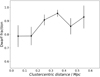 |
Fig. 16. Dwarf fraction as a function of the projected clustercentric distance. |
Choque-Challapa et al. (2021) analyze the dwarf fraction in 10 galaxy clusters (0.015 ≲ z ≲ 0.03) from the KIWICS survey (PIs R. Peletier and A. Aguerri). They consider as dwarf galaxies the individuals in the range −19.0 < Mr < −15.5 mag. The authors find dwarf fractions in all clusters ≳0.7. Moreover, they calculate the dwarf fraction in the same way for the well-studied Fornax and Virgo clusters, using the catalogs from Venhola et al. (2018) and Kim et al. (2014), finding it to be ∼0.7 for both. If we adopt the same definition as them, complementing again our catalog with the one by Christlein & Zabludoff (2003), we infer a dwarf fraction of 0.71, thus in prefect agreement with the fraction of the other nearby clusters, and consistent with Fornax and Virgo’s fractions. Table 4 summarizes the comparison.
Dwarf fractions in different clusters.
Choque-Challapa et al. (2021) find that in 5 out of 10 studied clusters the radial distributions of dwarf and giant are different. These cases correspond to the more massive clusters in their sample, and in these cases the giant galaxies are centrally more concentrated, a similar result to what we observe for Hydra I.
7.2. Colors of Hydra’s dwarf galaxies
In this section we aim at comparing the dwarf galaxy colors we computed for the Hydra I cluster, with the analog population in other local clusters, that is the Fornax and the Virgo clusters. The most complete dwarf galaxy sample to date in the Virgo cluster core, in terms of luminosity, is that of the NGVS (Ferrarese et al. 2012), presented in Ferrarese et al. (2020). For the Fornax cluster, we take as reference sample the dwarf catalog produced by the Fornax Deep Survey (Peletier et al. 2020), presented by Venhola et al. (2018).
In the color-magnitude diagram shown in Fig. 17, we compare the CMR of dwarf galaxies in Hydra I, with the red sequences (RS) of the Virgo and Fornax cluster cores (Roediger et al. 2017; Venhola et al. 2019, respectively). We use the g-band absolute magnitudes on the x-axis instead of the r-band, which is the one used in the analysis of the Virgo cluster by Roediger et al. (2017). For Hydra I’s CMR, we use the running mean of the color-magnitude relation for the early-type dwarf galaxies in our sample, selected as done for the r-band in Sect. 6.2. Roediger et al. (2017) analyzed the RS of the Virgo cluster core galaxies, up to ∼106 L⊙ (Mg ≃ −10 mag), finding the first evidence for a moderate flattening of the RS at the faint end, in different colors. Therefore, their RS has a shape which is better described by a double power law, with two different slopes, with a knee at Mg ≃ −14 mag. Venhola et al. (2019) did not derive the RS analytically, but rather showed the running means of the CMR within different radii from the center. To make a fair comparison, we consider their g − r vs. Mg relation only for dwarfs within 2Rcore (i.e. ∼0.5 Mpc, Ferguson 1989).
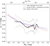 |
Fig. 17. Comparison between Hydra I color-magnitude relation in this work and the red sequence for the Virgo and Fornax clusters. The black line represents the running mean of the CMR for the Hydra I’s dwarfs in our sample, and the dotted lines show 1σ deviation (we use a fixed bin wide N = 30 individuals). The red dashed line is the CMR in the core of the Virgo cluster (Roediger et al. 2017). The blue dash-dotted line shows the Fornax CMR within 2Rcore (Venhola et al. 2019). |
The RS we present is, within the errors, in good agreement with the color-magnitude relations of both Fornax and Virgo clusters. The Fornax cluster RS matches the change in slope toward the faint luminosity of the Virgo cluster RS, while the Hydra I slope is relatively noisy for faint magnitudes, but consistent with such a flattening. Except for this point, we infer that the CMRs of the early-type galaxies are similar within the uncertainties in the Virgo, Fornax and Hydra I cluster cores.
LSB galaxies in the Coma cluster also show a range of color, and a color-magnitude relation, consistent with the CMR of Virgo, Fornax and Hydra I (Alabi et al. 2020). Bower et al. (1992) evidenced that there are no intrinsic differences between the CMRs of galaxies in Virgo and Coma. Detailed CMR analysis of three local clusters (namely A85, A496, A754) also confirm close agreement with that of the Coma cluster, and thus with Virgo, Fornax and Hydra I, (McIntosh et al. 2005). More in general, other observations suggested that such a red sequence exists in clusters over a wide redshift range (for instance 0.2 ≤ z ≤ 1.1, Bell et al. 2004), and our result provides further proof of its universality.
Comparing the cumulative radial distributions for Hydra I red and blue dwarfs (see Fig. 15), we can rule out with a good confidence degree the hypothesis that they are statistically similar, given the KS test p-value = 0.074. However, we note that red dwarf galaxies are located closer to the cluster center, with no blue dwarf galaxies within 0.15 Mpc projected distance. For what concerns the blue dwarfs fraction, we observed it to be ∼0.14. The fraction in Fornax, estimated in a similar way is 0.15, hence in prefect agreement with that of Hydra I. In the Virgo cluster, the fraction of blue dwarfs is instead larger, ∼0.3 (Venhola et al. 2019; Kim et al. 2014; Choque-Challapa et al. 2021). The similar dwarf fraction in Fornax and Hydra I clusters is intriguing, considering that Hydra I is more than twice as massive virial mass, and has a velocity dispersion almost two times higher (see Venhola et al. 2018, and therein references for a summary of Fornax properties).
7.3. Galaxy scaling relations in Local galaxy clusters
We show in Fig. 12 how dwarfs properties scale as a function of the total luminosity, finding that size, surface brightness and Sérsic index correlate with the dwarfs total magnitude.
In Fig. 18 we compare in detail the scaling relations with the analogous relations from other clusters. We compare the following clusters in the Local Universe: Virgo (sample from Ferrarese et al. 2020), Fornax (FDS dwarfs sample Venhola et al. 2019), Centaurus (Misgeld et al. 2009), Hydra I (in addition to our sample we included also Misgeld et al. 2008), and Coma (Alabi et al. 2020). There is general agreement between galaxies from different clusters. Considering the log(Re) vs. Mr plane, a linear relation is observed for dwarfs almost over every magnitude range. Starting from Mr ≃ −8 mag galaxies have increasing size with increasing luminosity up to Mr ≃ −13 mag. Then, in the range −13 ≲ Mr ≲ −17.5 mag there is a change in the slope of the relation, with Re growing slower as a function of the luminosity over this magnitude range. Brighter than −17.5 mag the slope changes again, and the size increases with higher luminosity. Also in less dense environments, a similar linear relation between log Re and total luminosity holds: Carlsten et al. (2021) report a similar relation for dwarf satellites in the Local Volume (D < 12 Mpc), that extends down to Re ≃ 100 pc and MV ≃ −7 mag. Poulain et al. (2021) reveal analogous behavior of dwarf galaxies located in the low to moderate density environments of the MATLAS fields.
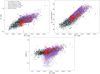 |
Fig. 18. Comparison of galaxies scaling relations among different Local Universe clusters. Top-left panel: effective radius vs. r-band magnitude (Mr). Top-right panel: mean effective surface brightness (r-band) as a function of the absolute r-band magnitude. Bottom panel: Sérsic index n as a function of Mr. The red circles represents Hydra I dwarf galaxies from our sample. The open blue triangles are the Fornax dwarfs (Venhola et al. 2019). The open orange diamonds indicate Hydra I early-types galaxies by Misgeld et al. (2008), while the green crosses represents Centaurus cluster galaxies (Misgeld et al. 2009). Empty black plus are Virgo galaxies (NGVS sample Ferrarese et al. 2020); open purple squares are Coma galaxies (Alabi et al. 2020). |
Looking at the  vs. Mr diagram (top-right panel of Fig. 18), galaxies occupy a well defined band which stretches from Mr ≃ −20 mag down to ≃ − 8 mag, with few outliers. The average scatter increases moderately toward fainter magnitudes. Again, this relationship holds also for dwarfs in less dense environments (Carlsten et al. 2021).
For the last scaling relation analyzed in Fig. 12, that is Sérsic index vs magnitude, we already mentioned the similarity between Hydra I’s galaxies and dwarfs in other local environments, both clusters and loose groups. In the bottom panel of Fig. 18 a detailed comparison of the n vs. total r-band magnitude is shown for galaxies of different clusters. The Sérsic index n varies with magnitude, on average increasing for brighter magnitudes. A mild flattening is observed only toward faintest luminosities (Mr < −11 mag). However, a much larger scatter and possibly a different slope is observed for galaxies in the Coma cluster, especially at −11 < Mr < −16 mag. Moreover, this relation also holds for early-type dwarf satellites around Milky Way-like galaxies, and for dwarfs in loose groups in the Local Universe. Indeed, Carlsten et al. (2021) observed in their sample the same trend for the early-type satellites in the stellar mass range 105.5 < M* < 108.5 M⊙. On average, the faintest dwarfs in the different environments are well represented by Sérsic profiles with 0.5 ≲ n ≲ 1, while bright ones are better represented by radial profiles with indices n > 1. This means that the most luminous dwarfs are more centrally concentrated, while less luminous ones have a flatter profile in the center.
From our analysis we conclude that photometric scaling relations are very similar across clusters of different characteristics. Indeed, Fornax, Virgo, Centaurus, Hydra I and Coma span a wide range of virial masses (from 1013 M⊙ to 1015 M⊙, Girardi et al. 1998), and radii (from 0.7 Mpc to 4 Mpc, Girardi et al. 1995), and they also have very different velocity dispersion (from ∼350 km s−1 to ∼1000 km s−1). Moreover, these four clusters show different structures, and some of them have a major segmentation in subgroups. However, from a photometric point of view, there is no observational evidence that the dwarf galaxies in these local clusters are different. Moreover, the same trends are observed also for dwarf satellites around Milky-Way like galaxies (Carlsten et al. 2020, 2021). These similarities may suggest that the evolution of the dwarf galaxies is somehow independent from the properties of the environment, and therefore that this is playing perhaps a marginal role.
7.4. Substructures in the Hydra I cluster
The smoothed map of the projected galaxy distribution shown in Fig. 9 suggests that the dwarf galaxies in the cluster are not uniformly distributed. The dwarf galaxies projected number density peaks close to the cluster core, off-center on the NW side to the region where the BCGs are located. The peak offset is of ≃5′ from the cluster center (represented by NGC 3311). In this region, also the X-ray emission is a bit more extended. Two more over-densities are found with respect to the cluster core, one on the N-NW and the other on the SE side, respectively (see Fig. 10). All these regions are dominated by the light from the brightest cluster members. Arnaboldi et al. (2012) pointed out that an entire group of small galaxies is falling through the cluster core, and they have already been partially dissolved by tidal interactions. Barbosa et al. (2018) has observed the sloshing of the central part of NGC 3311 with respect to the stellar halo. The velocity displacement of the cD vs. the baricenter of the cluster core indicate subcluster merging. This subcluster merging is consistent with the elongated loop-sided number distribution of dwarfs in the Hydra I core, as shown in Fig. 9.
The other two subgroups have different distributions. In the north side of the cluster core, cluster members are arranged in a filament-like structure, with galaxies extending along the SN direction. The projected distribution of the dwarf galaxies seems to be coherent with this structure. In the southern part of this structure, a dwarf galaxy (HCC 087) currently being tidally disrupted by the galaxy cluster’s potential itself was discovered, or, alternatively, by the nearby elliptical HCC 005 (Koch et al. 2012). On the SE side of the cluster, the brightest galaxy is NGC 3316, with a systemic velocity comparable to the galaxies in the core (that is cz ∼ 4000 km s−1) and a foreground group of galaxies, dominated by NGC 3312 and NGC 3314AB, which is falling into the cluster potential. The over-density found in the dwarf galaxy distribution is also consistent with these two substructures.
The presence of several substructures in the Hydra I cluster was also observed by Lima-Dias et al. (2021). Using two different approaches, they found possible subgroups of galaxies within the virial radius. Among these, two of the possible substructures are at a clustercentric distances of ∼0.2 Mpc and ∼0.3 Mpc, and within the errors they coincide with the two over-densities we report in the right panel of Fig. 9.
It was also observed that the cluster does not show a Gaussian velocity distribution, therefore substructures could be important in Hydra I. Fitchett & Merritt (1988) show that the velocity distribution within 40′ (∼600 kpc) from the cluster center has different peaks, one of which corresponds to the radial velocity of NGC 3312. The presence of small-scale substructures in dwarfs distribution, large ∼100 − 150 kpc, have also been observed in the Fornax cluster (Ordenes-Briceño et al. 2018). As for Hydra I, the Fornax galaxy number density does not to peak in the cluster center. Rather, the Fornax cD galaxy NGC 1399 occupies an apparent saddle-point between two main dwarf galaxy over-densities (see also Muñoz et al. 2015).
In conclusion, the 2D projected density distribution derived for the dwarf galaxies in the Hydra I cluster supports the idea that this environment is still in an active assembly phase, where several subgroups of galaxies are merging into the cluster potential.
To test whether or not the dwarfs close in projection to the cluster substructures have the same properties as those in the general cluster environment, we divided them into four groups, based on the smoothed map distribution. Specifically, we divided the dwarf galaxies in our catalog into the three mentioned substructures (core, north, and southeast groups), and in the remaining part of the studied field. As limit for the core group we considered the yellow contour in Fig. 9, which corresponds to the 0.1 probability density level (i.e. 10% of the probability mass will lie above the contour). We label galaxies as core galaxies if they are located, in projection, within a circle which circumscribes the yellow contour. For the N- and SE- group we choose the purple contour as density limit, which correspond to 0.25 probability density level. Given the less regular shape of these two contours, we choose box shape regions which completely include them. Again, projected location of galaxies is considered as group membership criterion. The three regions are chosen such that they do not overlap each other. Galaxies outside these three substructures are included in a fourth group, named “outside”.
We compare galaxy g − r color and Re in the four different structures. This choice is guided by the fact that the color is intrinsically linked to the underlying stellar population of the galaxy, while the Re indicates the galaxy’s size and light concentration. Thus, both color and Re are associated to the evolutionary processes acting on the dwarfs. The analysis is presented in Fig. 19, where we show g − r and Re as a function of the total r-band magnitude, and their distribution, for the different groups.
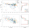 |
Fig. 19. Comparison between dwarf galaxies in different cluster substructures. Dwarfs not included in the three main subgroups are labeled as “Outside”. Top panels: the color-magnitude diagram is shown on the left, while the g − r color distributions are shown as histograms on the right panel. Symbol definitions are given in the legends. Bottom panels: on the left is reported the Re vs. Mr plane, while on the right are the Re distributions for dwarfs in the four substructures. |
The CMD in Fig. 19 shows that majority of the dwarfs located in projection within the cluster core follow the RS, and all but one have g − r ≳ 0.5 mag. Interestingly, we notice that the SE-group has the highest fraction of blue dwarfs (g − r ≤ 0.4 mag). However, no other significant difference emerges between dwarfs in the groups, and galaxies in projection outside the three main substructures. Also for what concerns the effective radius no clear difference is found between dwarfs belonging to different substructures.
Bearing in mind that the separation in groups is based on the projected location in the cluster, this result confirms what is pointed out in Sect. 7.3. Indeed, no major difference is found among galaxies in different substructures in our sample.
7.5. Origin of the clustercentric trends
In Fig. 14 we examine how the structural and physical properties of the dwarf galaxies in the Hydra I cluster core change as a function of the clustercentric distance. Details of the results are given in Sect. 6.5 but here it is important to observe that these clustercentric properties depend on the galaxy luminosity, i.e. on the galaxy stellar mass. This suggests that massive and low-mass dwarfs might be affected by different environmental processes, or that the relative importance of the environmental mechanisms depends on the dwarf galaxy mass.
We observe that Hydra I red dwarfs have, on average, g − r color getting redder with decreasing clustercentric distance, with a stronger correlation for brighter bins. Venhola et al. (2019) analyzed the same clustercentric trends for dwarf galaxies in the Fornax cluster, splitting dwarfs in 2 mag wide magnitude bins as we do. The authors report color’s trends which are consistent with our findings in the different magnitude bins. For the effective radii, we notice a weak positive correlation between with clustercentric distances for the high- and mid-luminosity dwarfs, but no clear trend is observed for the faintest dwarfs. Interestingly, Venhola et al. (2019) found that for the most luminous dwarfs Re decreases toward the inner parts of Fornax, in agreement with Hydra I dwarfs of comparable luminosity; for the faintest Fornax dwarfs the size increases going inward with a weak correlation. The latter result is not in agreement with the Hydra I faint dwarf galaxies.
Thanks to our in-depth spatially resolved photometrical analysis, we are now in the position to discuss what evolution mechanisms can be responsible for such clustercentric trends, and hence what is the role of the environment on cluster galaxies. The main processes involved in the transformation of galaxies from star forming to quiescent ETGs in clusters are galaxy harassment and ram-pressure stripping, introduced in Sect. 1. A direct observational consequence of ram pressure should be that a galaxy, with a given mass, would become redder with fainter  . From a structural point of view, the galaxy should not change its concentration, therefore Sérsic n and Re should not be affected. In the case of partial gas stripping, the process leads to a higher central surface brightness and increased central concentration of the light profile, if star formation results in the central region. As consequence of galaxy harassment, the light concentration of a galaxy increases (that is its central surface brightness), and because the star formation activity is generally quenched, it becomes redder. Thus, from an observational point of view, at a given mass, harassment slowly increases the Sérsic index n of galaxies, which become redder with brighter
  . Unfortunately, harassment and partial ram-pressure stripping have similar photometric effects on galaxies, making it very hard to distinguish between them.
To test whether Hydra I dwarf population show signs of ram-pressure and/or harassment, as predicted by theory, we analyze the correlation between g − r color and surface brightness, and concentration, for galaxies of different luminosities. In Fig. 20 we present this comparison, using the Sérsic index as indicator of light concentration. To better interpret the results we test statistically the correlation using the Spearman’s rank correlation test, which is reported in each panel of Fig. 20. Dwarf galaxies are binned in magnitude bins, as done for the clustercentric trends. We find that in each luminosity bin there is a negative correlation between color and  , which means galaxies become redder with increasing surface brightness. However, the correlation has increasing strength with increasing luminosity bins: it is robust for dwarfs with Mr < −16 mag, moderate for mid-luminosity dwarfs, and mild for low-luminosity dwarfs. In addition, to compare the trend between the surface brightness and color with the passive evolution of a single stellar population, we overlay the surface brightness vs. color evolutionary tracks on each panel of Fig. 20, using the models of Vazdekis et al. (2010). We use a Kroupa-like initial mass function (IMF), and show tracks for the following metallicities: [Z/H] = −1.79, −0.96, 0.06 dex. The ages range from 0.5 to 14 Gyr. The colors are predicted by the models, while initial surface brightness is set manually. Low-luminosity dwarfs show a
  vs. g − r relation that approximately follows the passive evolutionary tracks. Similarities can be found also for the mid-luminosity bin (−16.5 < Mr < −14.5 mag).
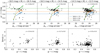 |
Fig. 20. Top panels: dwarf galaxies g − r colors as a function of the r-band mean effective surface brightness. Evolutionary tracks of single stellar population for a Kroupa-like IMF for different metallicities are shown. The crosses on each track correspond to 0.5, 1, 2, 3, …, 13, 14 Gyr. Horizontal lines show the 4 Gyr age level of each track. Lower panels: galaxies Sérsic indices n as a function of their colors. Galaxies are split in three luminosity bins, represented by the different columns. In each panel is reported the ρ value of the corresponding Spearman’s correlation test, and its error. |
Concerning the Sérsic index n, there is a moderate positive correlation in the first two magnitude bins (Mr < −14.5 mag), therefore the redder the galaxy, the higher the Sérsic index on average. By contrast, dwarfs in the faintest bin are consistent with no correlation, and dwarfs span over a wide range of Sérsic indices.
Interpreting these results in light of the theory predictions, we can conclude that mid- and high-luminosity Hydra I dwarfs (Mr < −14.5 mag) are mildly consistent with the harassment and/or partial ram-pressure scenarios.
Venhola et al. (2019) tested environmental mechanisms for Fornax dwarfs of different luminosity, as we do for Hydra I. They concluded that the most luminous galaxies (Mr < −16 mag) are consistent with being quenched via harassment and/or partial ram-pressure stripping, because they become redder with increasing concentration and surface brightness. Therefore, Hydra I and Fornax brighter dwarfs (Mr < −16 mag) are consistent with being affected by the same environmental processes. Janz et al. (2021) compared color vs mean effective surface brightness for Virgo and Fornax galaxies, binning them in magnitude bins too. They found that the color–surface brightness diagrams are remarkably similar for the two clusters; galaxies with M* > 108 M⊙ have constant or increasing g − r color with increasing surface brightness, as happens for the Hydra I most luminous dwarfs. On the other hand, they report that low-mass dwarfs (M* < 108 M⊙) show the opposite trend. However, when splitting the population in LTGs and ETGs, the authors found that only the low-mass LTGs are consistent with a fading and reddening following the quenching of star formation. For the ETGs there are no (or only weak) correlations between g − r and surface brightness in all mass bins. Discussing possible explanations for this discrepancy, Janz et al. (2021) concluded that the most likely scenario has to do with an early quenching (for example via gas removal), for which the current fading and reddening becomes less significant and less defined. This could mean that when the brightest dwarfs fall in clusters and loose their gas, they are able to keep some of it, which accumulates in their centers, forms stars, of higher metallicity, and then it makes the galaxy redder, and with an higher surface brightness.
The low-luminosity Hydra I dwarfs, while having on average redder colors with brighter surface brightness, do not show any increase in light concentration, as expected for harassment and partial gas stripping. However, they show a good agreement with passive evolutionary tracks of stellar population. Venhola et al. (2019) observed that the faintest dwarfs in Fornax (Mr > −14.5 mag) show a positive correlation between g − r color and  , while for the concentration vs. color relation there is a rather flat trend. Therefore, the quenching of the Fornax low-mass galaxies is consistent with complete gas-stripping and subsequent fading, as happening also for Virgo low-mass dwarfs (Janz et al. 2021). In this case, faint Hydra’s dwarfs seem to differ from Fornax ones, with the latter being more consistent with the full ram-pressure scenario. However, we cannot rule out the complete ram-pressure stripping for low-luminosity Hydra I dwarfs, and a more detailed analysis is required.
8. Summary and conclusions
This work generated a new catalog of resolved dwarf galaxies for the 56.7 × 46.6 arcmin2 central area in the Hydra I cluster, covering almost half its virial radius, from the deep multiband imaging data of the VEGAS survey. The catalog contains 317 galaxies fainter than Mr = −18.5 mag and with semi-major axis larger than a > 0.84 arcsec (∼200 pc at Hydra I’s distance), of which 61 were already present in Misgeld et al. (2008) catalog, and 70 in the work of Christlein & Zabludoff (2003). The detection efficiency reaches 50% at the limiting magnitude Mr = −11.5 mag, and at the mean effective surface brightness  mag arcsec−2. Using the new photometric catalog we analyzed the principal scaling relations and compared the results with the corresponding populations in other nearby galaxy clusters. Moreover, we investigated how these properties are affected by the surrounding environment, discussing the most likely mechanisms responsible for galaxy transformation. To this aim we studied how the different properties change as a function of the clustercentric distance, dividing the dwarf sample in bins of different magnitude.
The main results of this analysis are the following:
-
The dwarf galaxies are not uniformly distributed in the cluster, rather they are grouped in substructures in different locations across the covered area (Fig. 9). We recognized three over-densities of galaxies, a peak NW of the cluster core, a group north of the core, and another subgroup of galaxies in the SE region of the field. All these areas also overlap with the bright galaxy over-densities. Additionally, dwarfs and giants have radial distribution statistically different, with the former being less concentrated tan giants in the core.
-
The CMR derived from our observations is consistent with the previous CMR of Misgeld et al. (2008), and with the red sequence of other galaxy clusters in the local Universe (see Fig. 17).
-
Galaxies photometric scaling relations are very similar across Local Universe clusters with different properties (see Fig. 18). There is no observational evidence for dwarfs inhabiting Virgo, Fornax, Centaurus, Hydra I and Coma to be different from each other, from a photometrical and structural point of view.
-
From the clustercentric trends, we concluded that dwarf galaxies with Mr < −14.5 mag become redder toward the center of the cluster (Fig. 14), and become slightly larger with increasing distance from the center.
Based on these results we draw two main conclusions about the structure of the Hydra I cluster. The existence of subgroups of galaxies (dwarfs and giants) in the cluster is in agreement with previous findings by Lima-Dias et al. (2021), Arnaboldi et al. (2012), and Barbosa et al. (2018), and this suggests that the assembly of the cluster is still ongoing. The cluster environment transforms and influences the galaxies evolution, with the brightest and mid-luminosity dwarfs (Mr < −14.5 mag) being consistent with the effects of harassment and/or partial gas stripping.
We adopt a ΛCDM cosmology with Ωm = 0.3, ΩΛ = 0.7 and H0 = 72 km s−1 Mpc−1, Freedman et al. (2001).
For a full reference of all SEXTRACTOR’s flags see https://sextractor.readthedocs.io/en/latest/Flagging.html
This SEXTRACTOR’s parameter estimates the radius enclosing a certain quantity of the total object’s flux. In this case, we consider half of the total light.
Stars are injected according to an exponential law in the magnitude range 15 ≤ mr ≤ 23 mag. The total number of injected stars is approximately normalized by estimating -for the appropriate magnitude range- the total number of stellar detections from Gaia (Gaia Collaboration 2016) over the same area.
For further details see Sect. 7.1 Venhola et al. (2018).
Some examples are given in Bender et al. (2005) and Côté et al. (2006).
All magnitudes and colors are corrected for Galactic extinction using correcting values from Schlegel et al. (1998) and Schlafly & Finkbeiner (2011).
The increasing redshift dims the surface brightness too, but the contribution is relatively small for low and mid redshifts. The dimming factor is 1/(1 + z)4, that means that at Hydra I’s redshift z ∼ 0.01 there is ∼3% dimming.
The dwarf ratio is calculated as:
As number of giant galaxies we considered galaxies brighter than Mr = −18.5 mag which are spectroscopically confirmed Hydra I’s galaxies, taking them from Christlein & Zabludoff (2003).
X-ray data for Hydra I are taken from the XMM-Newton archive http://nxsa.esac.esa.int/nxsa-web/#search. The observation used are presented in Hayakawa et al. (2006).
The Spearman’s correlation test assesses how well the relationship between two variables can be described using a monotonic function. A perfect correlation is expressed by +1 and −1. Intuitively, negative values indicate decreasing monotonic correlation, while positive values indicate increasing monotonic correlation (Kokoska & Zwillinger 2000). Generally correlation above 0.4 are considered relatively strong; between 0.2 and 0.4 are moderate, and below 0.2 are consistent with no-correlation at all.
Acknowledgments
We thank the anonymous referee for his/her comments and constructive suggestions. This work is based on visitor mode observations collected at the European Southern Observatory (ESO) La Silla Paranal Observatory within the VST Guaranteed Time Observations, Programme ID: 099.B-0560(A). A.L.M. acknowledges financial support from the INAF-OAC. INAF authors acknowledge financial support for the VST project (P.I.: P. Schipani). D.A.F. thanks the ARC for supoort via DP200102574. G.D. acknowledges support from CONICYT project Basal AFB-170002, and FONDECYT REGULAR 1200495. C.S. is supported by an ‘Hintze Fellow’ at the Oxford Centre for Astrophysical Surveys, which is funded through generous support from the Hintze Family Charitable Foundation. This research made use of Astropy (http://www.astropy.org), a community-developed core Python package for Astronomy (Astropy Collaboration 2013, 2018).
References
- Alabi, A. B., Romanowsky, A. J., Forbes, D. A., Brodie, J. P., & Okabe, N. 2020, MNRAS, 496, 3182 [NASA ADS] [CrossRef] [Google Scholar]
- Arnaboldi, M., Ventimiglia, G., Iodice, E., Gerhard, O., & Coccato, L. 2012, A&A, 545, A37 [NASA ADS] [CrossRef] [EDP Sciences] [Google Scholar]
- Astropy Collaboration (Robitaille, T. P., et al.) 2013, A&A, 558, A33 [NASA ADS] [CrossRef] [EDP Sciences] [Google Scholar]
- Astropy Collaboration (Price-Whelan, A. M., et al.) 2018, AJ, 156, 123 [Google Scholar]
- Barbosa, C. E., Arnaboldi, M., Coccato, L., et al. 2018, A&A, 609, A78 [NASA ADS] [CrossRef] [EDP Sciences] [Google Scholar]
- Barbosa, C. E., Spiniello, C., Arnaboldi, M., et al. 2021, A&A, 649, A93 [NASA ADS] [CrossRef] [EDP Sciences] [Google Scholar]
- Bell, E. F., Wolf, C., Meisenheimer, K., et al. 2004, ApJ, 608, 752 [NASA ADS] [CrossRef] [Google Scholar]
- Bender, R., Kormendy, J., Bower, G., et al. 2005, ApJ, 631, 280 [NASA ADS] [CrossRef] [Google Scholar]
- Bertin, E., & Arnouts, S. 1996, A&AS, 117, 393 [NASA ADS] [CrossRef] [EDP Sciences] [Google Scholar]
- Bilicki, M., Hoekstra, H., Brown, M., et al. 2018, A&A, 616, A69 [NASA ADS] [CrossRef] [EDP Sciences] [Google Scholar]
- Binggeli, B., Sandage, A., & Tarenghi, M. 1984, AJ, 89, 64 [NASA ADS] [CrossRef] [Google Scholar]
- Binggeli, B., Sandage, A., & Tammann, G. 1985, AJ, 90, 1681 [NASA ADS] [CrossRef] [Google Scholar]
- Blakeslee, J. P., & Cantiello, M. 2018, Res. Notes Am. Astron. Soc., 2, 146 [Google Scholar]
- Bower, R. G., Lucey, J. R., & Ellis, R. S. 1992, MNRAS, 254, 601 [NASA ADS] [CrossRef] [Google Scholar]
- Bullock, J. S., & Boylan-Kolchin, M. 2017, ARA&A, 55, 343 [Google Scholar]
- Capaccioli, M., Spavone, M., Grado, A., et al. 2015, A&A, 581, A10 [NASA ADS] [CrossRef] [EDP Sciences] [Google Scholar]
- Carlsten, S. G., Beaton, R. L., Greco, J. P., & Greene, J. E. 2019, ApJ, 879, 13 [NASA ADS] [CrossRef] [Google Scholar]
- Carlsten, S. G., Greco, J. P., Beaton, R. L., & Greene, J. E. 2020, ApJ, 891, 144 [NASA ADS] [CrossRef] [Google Scholar]
- Carlsten, S. G., Greene, J. E., Greco, J. P., Beaton, R. L., & Kado-Fong, E. 2021, ApJ, 922, 267 [NASA ADS] [CrossRef] [Google Scholar]
- Choque-Challapa, N., Aguerri, J. A. L., Mancera Piña, P. E., et al. 2021, MNRAS, 507, 6045 [NASA ADS] [CrossRef] [Google Scholar]
- Christlein, D., & Zabludoff, A. I. 2003, ApJ, 591, 764 [Google Scholar]
- Côté, P., Piatek, S., Ferrarese, L., et al. 2006, ApJS, 165, 57 [Google Scholar]
- Djorgovski, S., & Davis, M. 1987, ApJ, 313, 59 [Google Scholar]
- Duc, P.-A., Cuillandre, J.-C., Karabal, E., et al. 2015, MNRAS, 446, 120 [Google Scholar]
- Eigenthaler, P., Puzia, T. H., Taylor, M. A., et al. 2018, ApJ, 855, 142 [Google Scholar]
- Faber, S., & Jackson, R. E. 1976, ApJ, 204, 668 [NASA ADS] [CrossRef] [Google Scholar]
- Ferguson, H. C. 1989, AJ, 98, 367 [Google Scholar]
- Ferrarese, L., Côté, P., Cuillandre, J.-C., et al. 2012, ApJS, 200, 4 [Google Scholar]
- Ferrarese, L., Cote, P., MacArthur, L. A., et al. 2020, ApJ, 890, 128 [NASA ADS] [CrossRef] [Google Scholar]
- Fitchett, M., & Merritt, D. 1988, ApJ, 335, 18 [NASA ADS] [CrossRef] [Google Scholar]
- Freedman, W. L., Madore, B. F., Gibson, B. K., et al. 2001, ApJ, 553, 47 [Google Scholar]
- Gaia Collaboration (Prusti, T., et al.) 2016, A&A, 595, A1 [NASA ADS] [CrossRef] [EDP Sciences] [Google Scholar]
- Gallart, C., Monelli, M., Mayer, L., et al. 2015, ApJ, 811, L18 [NASA ADS] [CrossRef] [Google Scholar]
- Geha, M., Blanton, M., Yan, R., & Tinker, J. 2012, ApJ, 757, 85 [NASA ADS] [CrossRef] [Google Scholar]
- Girardi, M., Biviano, A., Giuricin, G., Mardirossian, F., & Mezzetti, M. 1995, ApJ, 438, 527 [NASA ADS] [CrossRef] [Google Scholar]
- Girardi, M., Borgani, S., Giuricin, G., Mardirossian, F., & Mezzetti, M. 1998, ApJ, 506, 45 [NASA ADS] [CrossRef] [Google Scholar]
- Grado, A., Capaccioli, M., Limatola, L., & Getman, F. 2012, Mem. Soc. Astron. It. Suppl., 19, 362 [Google Scholar]
- Greco, J. P., van Dokkum, P., Danieli, S., Carlsten, S. G., & Conroy, C. 2021, ApJ, 908, 24 [NASA ADS] [CrossRef] [Google Scholar]
- Gunn, J. E., & Gott, J. R., III 1972, ApJ, 176, 1 [Google Scholar]
- Habas, R., Marleau, F. R., Duc, P.-A., et al. 2020, MNRAS, 491, 1901 [NASA ADS] [Google Scholar]
- Hamraz, E., Peletier, R. F., Khosroshahi, H., et al. 2019, A&A, 625, A94 [NASA ADS] [CrossRef] [EDP Sciences] [Google Scholar]
- Häussler, B., McIntosh, D. H., Barden, M., et al. 2007, ApJS, 172, 615 [Google Scholar]
- Hayakawa, A., Furusho, T., Yamasaki, N. Y., Ishida, M., & Ohashi, T. 2004, PASJ, 56, 743 [NASA ADS] [Google Scholar]
- Hayakawa, A., Hoshino, A., Ishida, M., et al. 2006, PASJ, 58, 695 [NASA ADS] [Google Scholar]
- Hermosa Muñoz, L., Taibi, S., Battaglia, G., et al. 2020, A&A, 634, A10 [NASA ADS] [CrossRef] [EDP Sciences] [Google Scholar]
- Hilker, M., Richtler, T., Barbosa, C. E., et al. 2018, A&A, 619, A70 [NASA ADS] [CrossRef] [EDP Sciences] [Google Scholar]
- Hodges, J. L. 1958, Arkiv för Matematik, 3, 469 [CrossRef] [Google Scholar]
- Hoyos, C., den Brok, M., Kleijn, G. V., et al. 2011, MNRAS, 411, 2439 [NASA ADS] [CrossRef] [Google Scholar]
- Iodice, E., Capaccioli, M., Grado, A., et al. 2016, ApJ, 820, 42 [Google Scholar]
- Iodice, E., Spavone, M., Cattapan, A., et al. 2020a, A&A, 635, A3 [NASA ADS] [CrossRef] [EDP Sciences] [Google Scholar]
- Iodice, E., Cantiello, M., Hilker, M., et al. 2020b, A&A, 642, A48 [EDP Sciences] [Google Scholar]
- Iodice, E., Spavone, M., Raj, M. A., et al. 2021, ArXiv e-prints [arXiv:2102.04950] [Google Scholar]
- Janz, J., Laurikainen, E., Lisker, T., et al. 2014, ApJ, 786, 105 [Google Scholar]
- Janz, J., Salo, H., Su, A. H., & Venhola, A. 2021, A&A, 647, A80 [NASA ADS] [CrossRef] [EDP Sciences] [Google Scholar]
- Kacharov, N., Battaglia, G., Rejkuba, M., et al. 2017, MNRAS, 466, 2006 [Google Scholar]
- Kim, S., Rey, S.-C., Jerjen, H., et al. 2014, ApJS, 215, 22 [Google Scholar]
- Koch, A., Burkert, A., Rich, R. M., et al. 2012, ApJ, 755, L13 [Google Scholar]
- Kokoska, S., & Zwillinger, D. 2000, CRC Standard Probability and Statistics Tables and Formulae (CRC Press) [Google Scholar]
- Kormendy, J. 1977, ApJ, 218, 333 [NASA ADS] [CrossRef] [Google Scholar]
- Kostov, A., & Bonev, T. 2018, Bulg. Astron. J., 28, 3 [Google Scholar]
- Kuijken, K. 2011, The Messenger, 146, 8 [NASA ADS] [Google Scholar]
- Leaman, R., Venn, K., Brooks, A., et al. 2014, Mem. Soc. Astron. It., 85, 504 [NASA ADS] [Google Scholar]
- Lima-Dias, C., Monachesi, A., Torres-Flores, S., et al. 2021, MNRAS, 500, 1323 [Google Scholar]
- Lisker, T., Glatt, K., Westera, P., & Grebel, E. K. 2006, AJ, 132, 2432 [Google Scholar]
- Loewenstein, M., & Mushotzky, R. 1996, ApJ, 471, L83 [NASA ADS] [CrossRef] [Google Scholar]
- Lupton, R., Blanton, M. R., Fekete, G., et al. 2004, PASP, 116, 133 [NASA ADS] [CrossRef] [Google Scholar]
- Mancillas, B., Duc, P.-A., Combes, F., et al. 2019, A&A, 632, A122 [NASA ADS] [CrossRef] [EDP Sciences] [Google Scholar]
- Mastropietro, C., Moore, B., Mayer, L., et al. 2005, MNRAS, 364, 607 [Google Scholar]
- McGlynn, T. A. 1990, Dynamics and Interactions of Galaxies (Springer), 225 [CrossRef] [Google Scholar]
- McIntosh, D. H., Zabludoff, A. I., Rix, H.-W., & Caldwell, N. 2005, ApJ, 619, 193 [NASA ADS] [CrossRef] [Google Scholar]
- Michea, J., Pasquali, A., Smith, R., et al. 2021, AJ, 161, 268 [NASA ADS] [CrossRef] [Google Scholar]
- Mieske, S., Hilker, M., & Infante, L. 2003, A&A, 403, 43 [NASA ADS] [CrossRef] [EDP Sciences] [Google Scholar]
- Mieske, S., Hilker, M., & Infante, L. 2005, A&A, 438, 103 [NASA ADS] [CrossRef] [EDP Sciences] [Google Scholar]
- Misgeld, I., Mieske, S., & Hilker, M. 2008, A&A, 486, 697 [NASA ADS] [CrossRef] [EDP Sciences] [Google Scholar]
- Misgeld, I., Hilker, M., & Mieske, S. 2009, A&A, 496, 683 [NASA ADS] [CrossRef] [EDP Sciences] [Google Scholar]
- Misgeld, I., Mieske, S., Hilker, M., et al. 2011, A&A, 531, A4 [NASA ADS] [CrossRef] [EDP Sciences] [Google Scholar]
- Moore, B., Katz, N., Lake, G., Dressler, A., & Oemler, A. 1996, Nature, 379, 613 [Google Scholar]
- Moore, B., Lake, G., & Katz, N. 1998, ApJ, 495, 139 [Google Scholar]
- Muñoz, R. P., Eigenthaler, P., Puzia, T. H., et al. 2015, ApJ, 813, L15 [Google Scholar]
- Ordenes-Briceño, Y., Eigenthaler, P., Taylor, M. A., et al. 2018, ApJ, 859, 52 [Google Scholar]
- Peletier, R., Iodice, E., Venhola, A., et al. 2020, ArXiv e-prints [arXiv:2008.12633] [Google Scholar]
- Peng, C. Y., Ho, L. C., Impey, C. D., & Rix, H.-W. 2002, AJ, 124, 266 [Google Scholar]
- Peng, Y.-J., Lilly, S. J., Kovač, K., et al. 2010a, ApJ, 721, 193 [Google Scholar]
- Peng, C. Y., Ho, L. C., Impey, C. D., & Rix, H.-W. 2010b, AJ, 139, 2097 [Google Scholar]
- Peng, Y.-J., Lilly, S. J., Renzini, A., & Carollo, M. 2012, ApJ, 757, 4 [NASA ADS] [CrossRef] [Google Scholar]
- Peng, Y.-J., Lilly, S. J., Renzini, A., & Carollo, M. 2014, ApJ, 790, 95 [NASA ADS] [CrossRef] [Google Scholar]
- Pillepich, A., Springel, V., Nelson, D., et al. 2018, MNRAS, 473, 4077 [Google Scholar]
- Popesso, P., Biviano, A., Böhringer, H., & Romaniello, M. 2006, A&A, 445, 29 [NASA ADS] [CrossRef] [EDP Sciences] [Google Scholar]
- Poulain, M., Marleau, F. R., Habas, R., et al. 2021, MNRAS, 506, 5494 [NASA ADS] [CrossRef] [Google Scholar]
- Price, J., Phillipps, S., Huxor, A., et al. 2009, MNRAS, 397, 1816 [NASA ADS] [CrossRef] [Google Scholar]
- Richter, O. G. 1987, A&AS, 67, 237 [NASA ADS] [Google Scholar]
- Richter, O. G., Materne, J., & Huchtmeier, W. K. 1982, A&A, 111, 193 [NASA ADS] [Google Scholar]
- Roediger, J. C., Ferrarese, L., Côté, P., et al. 2017, ApJ, 836, 120 [Google Scholar]
- Sánchez-Janssen, R., Aguerri, J. A. L., & Muñoz-Tuñón, C. 2008, ApJ, 679, L77 [CrossRef] [Google Scholar]
- Sasaki, S. S., Taniguchi, Y., Scoville, N., et al. 2007, ApJS, 172, 511 [NASA ADS] [CrossRef] [Google Scholar]
- Schaye, J., Crain, R. A., Bower, R. G., et al. 2015, MNRAS, 446, 521 [Google Scholar]
- Schipani, P., Noethe, L., Arcidiacono, C., et al. 2012, J. Opt. Soc. Am. A, 29, 1359 [Google Scholar]
- Schlafly, E. F., & Finkbeiner, D. P. 2011, ApJ, 737, 103 [Google Scholar]
- Schlegel, D. J., Finkbeiner, D. P., & Davis, M. 1998, ApJ, 500, 525 [Google Scholar]
- Smith, R., Sánchez-Janssen, R., Beasley, M. A., et al. 2015, MNRAS, 454, 2502 [Google Scholar]
- Springel, V., White, S. D. M., Jenkins, A., et al. 2005, Nature, 435, 629 [Google Scholar]
- Su, A. H., Salo, H., Janz, J., et al. 2021, A&A, 647, A100 [EDP Sciences] [Google Scholar]
- Tamura, T., Makishima, K., Fukazawa, Y., Ikebe, Y., & Xu, H. 2000, ApJ, 535, 602 [NASA ADS] [CrossRef] [Google Scholar]
- Tonry, J., & Schneider, D. P. 1988, AJ, 96, 807 [Google Scholar]
- Vazdekis, A., Sánchez-Blázquez, P., Falcón-Barroso, J., et al. 2010, MNRAS, 404, 1639 [NASA ADS] [Google Scholar]
- Venhola, A., Peletier, R., Laurikainen, E., et al. 2017, A&A, 608, A142 [NASA ADS] [CrossRef] [EDP Sciences] [Google Scholar]
- Venhola, A., Peletier, R., Laurikainen, E., et al. 2018, A&A, 620, A165 [NASA ADS] [CrossRef] [EDP Sciences] [Google Scholar]
- Venhola, A., Peletier, R., Laurikainen, E., et al. 2019, A&A, 625, A143 [EDP Sciences] [Google Scholar]
- Ventimiglia, G., Arnaboldi, M., & Gerhard, O. 2011, A&A, 528, A24 [NASA ADS] [CrossRef] [EDP Sciences] [Google Scholar]
- Visvanathan, N., & Sandage, A. 1977, ApJ, 216, 214 [Google Scholar]
Appendix A: Estimates of uncertainties
To estimate more realistic errors on the fitted parameters we use an approach based on mock galaxies, following the works of Venhola et al. (2017), Venhola et al. (2018), and Hoyos et al. (2011). The photometric measurements we carried out have uncertainties arising from two different sources: the brightest galaxies usually show more structures than the simple single Sérsic profile assumed by the models we used, while at the low surface brightness end we are limited by the signal-to-noise. In order to characterize the typical uncertainties of the fit parameters, we make photometric measurements for a bunch of detected mock galaxies, generated as described in Sec. 3.2. Specifically, 400 detected mock galaxies, having a wide range of structural properties, went through the same photometric pipeline as the real galaxies. In Figure A.1 we show a comprehensive comparison between the original mock galaxies parameters, and the measured ones. We also plot there the average differences between input and output parameters. As expected, for all parameters the deviations of the measured values from the original ones increase toward lower surface brightness galaxies. In the case of the effective radius this is more evident, indeed for larger Re values GALFIT tends to underestimate considerably the size of the galaxies.
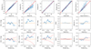 |
Fig. A.1. Comparison between True and measured properties of 400 mock galaxies. Top row panels: Comparison between the input structural parameters of the mock galaxies, and the values measured by the photometric pipeline. The parameters compared are: apparent magnitude (mr), effective radius (Re), position angle (Θ), axis ratio (b/a), and Sérsic index (n). The red solid lines represent the 1:1 ideal ratio. Mid and bottom row panels: The blue lines are the running means of the differences between the input and output parameters, as a function of their input and output |

To estimate the uncertainties, we fit the standard deviations of the input-output residuals, defined as
 (A.1)
(A.1)
where N is the number of mock galaxies in a given  bin. Similar to Venhola et al. (2017), Venhola et al. (2018), and Hoyos et al. (2011), we fit the σ with the function
 (A.2)
(A.2)
where α and β are the free parameters, and  is the mean effective surface brightness obtained by the photometric pipeline. Fitting results are listed in Table A.1, and are represented by the red dotted lines in the last row of Fig. A.1. We point out that these uncertainties measured empirically are larger than the standard uncertainties given by GALFIT. Our results are in good agreement with the ones obtained with same procedure by Venhola et al. (2017) and Venhola et al. (2018). The errors derived in this way for individual galaxies are given with their photometric parameters in the catalog.
Fit parameters of Eq. (A.2).
Appendix B: Band conversion
In this paper we worked with SDSS g and r photometric bands, but we extensively compared with works that used different photometric systems. To convert quantities from the Johnson V, R and I filters, to SDSS r and g we used the following equation listed in Kostov & Bonev (2018):
 (B.1)
(B.1)
 (B.2)
(B.2)
 (B.3)
(B.3)
 (B.4)
(B.4)
Appendix C: The Hydra I galaxy cluster dwarf catalog
We show in Table C.1 an example table from the Hydra I galaxy cluster dwarf catalog (HCDC). The full catalog is available at the CDS. In the table, we provide also the parameters’ errors.
An example table of our Hydra I dwarf galaxies catalog.
All Tables
Main configuration parameters used in SEXTRACTOR for the three different classes of sources.
Median values of the principal photometric parameters for the 30 missed objects from the Misgeld et al. (2008) Hydra I catalog.
All Figures
|
Fig. 1. Color composite image (g and r bands) of the VST mosaic’s portion used in this paper (56.7 × 46.6 arcmin2). The two cD galaxies NGC 3311 and NGC 3309, which lie in the cluster center, are labeled in the figure. Close to them, to the left is marked NGC 3312, a large spiral galaxy. Residual light from the two subtracted stars is still visible. North is up, and east is on the left. The color RGB image is created using the Lupton et al. (2004) scheme, using the r-band image as R filter input, the g-band as B filter input, and the average image between r and g bands as G filter input. |
| In the text | |
|
Fig. 2. Flux radius in arcsec vs. r-band magnitude. A tight band extends horizontally from mr ∼ 14 mag to ∼22 mag, and it is inhabited by stars. Extended objects are arranged in a more diffuse way. |
| In the text | |
|
Fig. 3. Size-magnitude diagram for detected sources, with size in pixels. Green dots represents the galaxies selected for the final clean catalog, i.e. have semi-major axis larger than 4 pixels, and have passed all the previous steps. |
| In the text | |
|
Fig. 4. Detection efficiency (number of detected galaxies over number of generated ones in the same bin) of our detection algorithm is shown color-coded such that red means more efficient, while blue less efficient. The efficiency is plotted for effective radius (Re, the pixel scale is 0.21 arcsec pix−1), axis ratio (b/a), and Sérsic index n, as function of mean effective surface brightness, without (top row) and with (bottom row) minimum size limit. The white lines show the 50% detection efficiency limit. |
| In the text | |
|
Fig. 5. Color selection criteria used to separate the cluster members from the background galaxies. The horizontal dotted line represents the upper color limit we applied, g − r = 0.95 mag: galaxies in the shaded gray area are excluded. The two BCGs are marked with black triangles. |
| In the text | |
|
Fig. 6. Scaling relations used for the galaxy selection. Left panel: mean effective surface brightness vs total magnitude (r-band) plane for catalog objects that passed the first selection cut. The black solid line is the linear fit of the redshift confirmed cluster members. The data of Christlein & Zabludoff (2003) are represented by red open circles. The dotted line indicates 2 standard deviations from the cluster sequence: the objects in the shaded gray area are removed from the sample. Right panel: color-magnitude diagram for galaxies that passed the first two cuts. Orange triangles are early-type galaxies found by Misgeld et al. (2008), and the orange solid line is their CMR. The dashed line is the 2 rms level we use to define galaxies as members of the Hydra I cluster. |
| In the text | |
|
Fig. 7. r-band images of the galaxies as they are classified in the visual inspection phase. Green bars are of equal length in each cutout, 10 arcsec. Background galaxies show spiral features, but they are considerably smaller than the Late-type galaxies that inhabit the cluster. The difference between the LTGs and the ETGs with structures in our classification scheme is mainly given by the color, hence is not evident in gray-scale images. |
| In the text | |
|
Fig. 8. Spatial distribution of the likely Hydra I cluster dwarfs in our sample (orange circles), and giant galaxies from Christlein & Zabludoff (2003), green triangles. The dividing magnitude is at Mr = −18.5 mag. The black circle indicates the cluster core radius rc = 170 h−1 kpc (Girardi et al. 1995), assuming h = 0.72, and the gray area indicates our studied field. The two BCGs, NGC 3311 and NGC 3309 are marked separately as black triangles. The two magenta stars show the position of the two major saturated stars that we masked. In the figure north is up and east is left. |
| In the text | |
|
Fig. 9. Projected galaxy density distribution inside the Hydra I cluster. Left panel: smoothed number density distribution of the galaxies in the Hydra I galaxy cluster. The observed galaxy distribution is convolved with a Gaussian kernel with σ = 10′. The colored contours highlight the iso-density curves (red, yellow and purple). X-ray contours (thin black lines) are also overlaid to the map. The two giant galaxies at the center of the cluster are represented by the two black triangles, while the magenta stars are the two modeled stars in the field. North is up, east is left. Right panel: projected galaxy surface density, as number of galaxies per square Mpc, plotted against the projected clustercentric distance. Red solid line is the density profile accounting for the area of the two saturated stars, while blue dashed line is the profile without correcting for that area. |
| In the text | |
|
Fig. 10. Cumulative functions of the clustercentric distances of giants (Christlein & Zabludoff 2003), green solid line, and of dwarfs, orange dashed line. The label refers to the p-value from the Kolmogorov–Smirnov test. The KS-test result states that the two radial distributions are statistically different. |
| In the text | |
|
Fig. 11. Color-magnitude relation for all Hydra I dwarf galaxies in our catalog. The solid line is the linear fit of the red sequence (Eq. (1)), while the dotted lines are the 2σ deviations from the fit. The two galaxy populations: blue triangles form the blue dwarf population, while red dots are the red dwarfs, with their color errors. |
| In the text | |
|
Fig. 12. From the top to the bottom row: effective radius Re, mean effective surface brightness in r-band |
| In the text | |
|
Fig. 13. Axis ratio distributions for the red and blue galaxies, represented by the red solid line, and by the blue dashed line, respectively. Top panel: cumulative distributions of the two populations. The black diagonal line shows a flat b/a distribution. The reported value is the p-value of the performed KS test. Bottom panel: fraction of red and blue dwarfs in b/a = 0.1 wide bins. |
| In the text | |
|
Fig. 14. Structural parameters of Hydra’s dwarf galaxies as a function of their projected clustercentric distance. Panel rows from top to bottom show: g − r color, effective radius Re, mean effective surface brightness |
| In the text | |
|
Fig. 15. Cumulative clustercentric distributions for both red and blue dwarfs, represented by a red solid line and a blue dashed line, respectively. The number on the bottom is the p-value of the performed KS test. |
| In the text | |
|
Fig. 16. Dwarf fraction as a function of the projected clustercentric distance. |
| In the text | |
|
Fig. 17. Comparison between Hydra I color-magnitude relation in this work and the red sequence for the Virgo and Fornax clusters. The black line represents the running mean of the CMR for the Hydra I’s dwarfs in our sample, and the dotted lines show 1σ deviation (we use a fixed bin wide N = 30 individuals). The red dashed line is the CMR in the core of the Virgo cluster (Roediger et al. 2017). The blue dash-dotted line shows the Fornax CMR within 2Rcore (Venhola et al. 2019). |
| In the text | |
|
Fig. 18. Comparison of galaxies scaling relations among different Local Universe clusters. Top-left panel: effective radius vs. r-band magnitude (Mr). Top-right panel: mean effective surface brightness (r-band) as a function of the absolute r-band magnitude. Bottom panel: Sérsic index n as a function of Mr. The red circles represents Hydra I dwarf galaxies from our sample. The open blue triangles are the Fornax dwarfs (Venhola et al. 2019). The open orange diamonds indicate Hydra I early-types galaxies by Misgeld et al. (2008), while the green crosses represents Centaurus cluster galaxies (Misgeld et al. 2009). Empty black plus are Virgo galaxies (NGVS sample Ferrarese et al. 2020); open purple squares are Coma galaxies (Alabi et al. 2020). |
| In the text | |
|
Fig. 19. Comparison between dwarf galaxies in different cluster substructures. Dwarfs not included in the three main subgroups are labeled as “Outside”. Top panels: the color-magnitude diagram is shown on the left, while the g − r color distributions are shown as histograms on the right panel. Symbol definitions are given in the legends. Bottom panels: on the left is reported the Re vs. Mr plane, while on the right are the Re distributions for dwarfs in the four substructures. |
| In the text | |
|
Fig. 20. Top panels: dwarf galaxies g − r colors as a function of the r-band mean effective surface brightness. Evolutionary tracks of single stellar population for a Kroupa-like IMF for different metallicities are shown. The crosses on each track correspond to 0.5, 1, 2, 3, …, 13, 14 Gyr. Horizontal lines show the 4 Gyr age level of each track. Lower panels: galaxies Sérsic indices n as a function of their colors. Galaxies are split in three luminosity bins, represented by the different columns. In each panel is reported the ρ value of the corresponding Spearman’s correlation test, and its error. |
| In the text | |
|
Fig. A.1. Comparison between True and measured properties of 400 mock galaxies. Top row panels: Comparison between the input structural parameters of the mock galaxies, and the values measured by the photometric pipeline. The parameters compared are: apparent magnitude (mr), effective radius (Re), position angle (Θ), axis ratio (b/a), and Sérsic index (n). The red solid lines represent the 1:1 ideal ratio. Mid and bottom row panels: The blue lines are the running means of the differences between the input and output parameters, as a function of their input and output |
| In the text | |
Current usage metrics show cumulative count of Article Views (full-text article views including HTML views, PDF and ePub downloads, according to the available data) and Abstracts Views on Vision4Press platform.
Data correspond to usage on the plateform after 2015. The current usage metrics is available 48-96 hours after online publication and is updated daily on week days.
Initial download of the metrics may take a while.