| Issue |
A&A
Volume 659, March 2022
|
|
|---|---|---|
| Article Number | A9 | |
| Number of page(s) | 23 | |
| Section | Stellar atmospheres | |
| DOI | https://doi.org/10.1051/0004-6361/202141738 | |
| Published online | 25 February 2022 | |
The earliest O-type eclipsing binary in the Small Magellanic Cloud, AzV 476: A comprehensive analysis reveals surprisingly low stellar masses
1
Institut für Physik und Astronomie, Universität Potsdam,
Karl-Liebknecht-Str. 24/25,
14476
Potsdam,
Germany
e-mail: This email address is being protected from spambots. You need JavaScript enabled to view it.
2
Armagh Observatory and Planetarium,
College Hill,
Armagh
BT61 9DG,
Northern Ireland,
UK
3
Astronomisches Rechen-Institut, Zentrum für Astronomie der Universität Heidelberg,
Mönchhofstr. 12-14,
69120
Heidelberg,
Germany
4
Institute of Astronomy, KU Leuven,
Celestijnenlaan 200D,
3001
Leuven,
Belgium
5
Department of Physics and Astronomy, University College London,
Gower Street,
London
WC1E 6BT,
UK
6
Centro de Astrobiología. CSIC-INTA. Campus ESAC.
Camino bajo del castillo s/n.
28 692
Villanueva de la Cañada,
Madrid,
Spain
Received:
7
July
2021
Accepted:
7
January
2022
Abstract
Context. Massive stars at low metallicity are among the main feedback agents in the early Universe and in present-day star forming galaxies. When in binaries, these stars are potential progenitors of gravitational-wave events. Knowledge of stellar masses is a prerequisite to understanding evolution and feedback of low-metallicity massive stars.
Aims. Using abundant spectroscopic and photometric measurements of an outstandingly bright eclipsing binary, we compare its dynamic, spectroscopic, and evolutionary mass estimates and develop a binary evolution scenario.
Methods. We comprehensively studied the eclipsing binary system, AzV 476, in the Small Magellanic Cloud (SMC). The light curve and radial velocities were analyzed to obtain the orbital parameters. The photometric and spectroscopic data in the UV and optical were analyzed using the Potsdam Wolf–Rayet (PoWR) model atmospheres. The obtained results are interpreted using detailed binary-evolution tracks including mass transfer.
Results. AzV 476 consists of an O4 IV-III((f))p primary and an O9.5: Vn secondary. Both components have similar current masses (20 M⊙ and 18 M⊙) obtained consistently from both the orbital and spectroscopic analysis. The effective temperatures are 42 kK and 32 kK, respectively. The wind mass-loss rate of log(Ṁ∕(M⊙ yr−1)) = −6.2 of the primary is a factor of ten higher than a recent empirical prescription for single O stars in the SMC. Only close-binary evolution with mass transfer can reproduce the current stellar and orbital parameters, including orbital separation, eccentricity, and the rapid rotation of the secondary. The binary evolutionary model reveals that the primary has lost about half of its initial mass and is already core helium burning.
Conclusions. Our comprehensive analysis of AzV 476 yields a consistent set of parameters and suggests previous case B mass transfer. The derived stellar masses agree within their uncertainties. The moderate masses of AzV 476 underline the scarcity of bright massive stars in the SMC. The core helium burning nature of the primary indicates that stripped stars might be hidden among OB-type populations.
Key words: binaries: eclipsing / binaries: spectroscopic / binaries: close / early-type / stars: fundamental parameters / stars: individual: AzV 476
© ESO 2022
1 Introduction
The most important parameter defining the evolution of a star is its mass. An often reported problem in stellar astrophysics is the “mass discrepancy” problem, which refers to the inconsistent masses derived from spectroscopy, evolutionary tracks, and, for binaries, from orbital motions (Herrero et al. 1992; Weidner & Vink 2010; Markova & Puls 2015). The analysis of O-type stars located in the Galaxy and the Large Magellanic Cloud (LMC) performed by Weidner & Vink (2010) reveal good agreement between the aforementioned mass estimates, but the study of Markova et al. (2018) suggests a mass discrepancy. Mahy et al. (2020) investigate a sample of O-type binaries in the LMC and find good agreement between spectroscopic and dynamic mass estimates while the evolutionary masses are at odds. These latter authors suggest previous binary interactions as a possible solution for this discrepancy.
However, the mass discrepancy problem has not yet been studied at metallicities lower than ≲ 1∕2 Z⊙. Sufficiently low metallicity is offered by the nearby Small Magellanic Cloud (SMC) galaxy (ZSMC ≈ 1∕7 Z⊙; Hunter et al. 2007; Trundle et al. 2007). Precise stellar masses in the SMC allow us to tackle questions about stellar evolution and feedback at low metallicity.
Stars with spectral types around O2–4 are expected to be very massive with M*≳ 50 M⊙ (Martins & Palacios 2021). However, the true masses of the early-type O stars are only poorly known, and therefore spectral types and masses might be falsely mapped. So far, only a couple of the SMC eclipsing binaries with early spectral types have been studied. Morrell et al. (2003) investigated the O6V+O4/5III(f) system Hodge 53-47 (alias MOA J010321.3-720538) and found dynamic masses of ≈ 26 M⊙ and ≈ 16 M⊙ for the primary and secondary, respectively. The eclipsing binary, OGLE SMC-SC10 108086, studied by Abdul-Masih et al. (2021) contains even less massive stars with ≈17 M⊙ and ≈14 M⊙. Only one eclipsing multiple stellar system in the SMC, HD 5980, appears to contain stars with masses ≳ 30 M⊙. Koenigsberger et al. (2014) and Hillier et al. (2019) studied this system in detail and found an inner eclipsing binary consisting of an LBV and a Wolf–Rayet (WR) star, and a third O-type supergiant star with a potential fourth companion. The orbital masses of the LBV and the WR star are≈61 M⊙ and ≈66 M⊙, respectively.Koenigsberger et al. (2014) suggest that there was little or no mass transfer, and that the WR star has formed via quasi-chemically homogeneous evolution. These examples highlight the complexity of massive star evolution and the need for advanced studies on the mass discrepancy problem in the high-mass regime.
For single stars, mass estimates rely on spectroscopic diagnostics or comparison with evolutionary tracks. Currently, standard stellar evolutionary models predict that the most massive stars, either single or in binary systems, start their lives on the main sequence (MS) as early-type O stars. Single stars expand and evolve away from the MS. During this phase, stars undergo strong mass loss where they might lose their entire hydrogen-rich envelope, revealing the helium core and becoming WR stars. In the case of closebinaries, evolutionary models predict that the expanding star is likely to interact with its companion. In the majority of cases, the expanding star will transfer its envelope to the companion, and become a binary-stripped helium star, possibly also with a WR-type spectrum (Dionne & Robert 2006; Shenar et al. 2020; Götberg et al. 2020).
The SMC hosts a handful of WR stars that have relatively high masses ranging from 10 M⊙ to 60 M⊙ (Shenar et al. 2016). These stars are so massive that their hydrogen-burning progenitors must have been early O-type (or WNL/Of) stars. However, in their recent study of the SMC OB-type population, Ramachandran et al. (2019) reveal a strong deficiency of massive stars (>30 M⊙) close to the MS in the upper part of the empiric Hertzsprung-Russell diagram (HRD) (see Holgado et al. 2020; Ramachandran et al. 2018, for studies of Galactic and the LMC O star populations). O-type stars are hot and luminous and are therefore easily detectable. Hence, a paucity of the earliest O-type stars in the SMC cannot be explained either by selection effects or stellar evolution scenarios (Schootemeijer et al. 2021). Thus, the deficiency of most massive O stars strongly questions the formation process of the WR stars in the SMC, as well as our basic understanding of stellar evolution in low-metallicity environments. In this context it is crucial to quantify the budget of massive stars (≳ 30 M⊙) in the SMC.
Poorly constrained processes that affect the lives of massive stars include radiatively driven winds, stellar envelope inflation, core overshooting, and rotationally induced internal mixing. In particular their dependence on mass and metallicity are not yet fully understood. These effects can drastically alter the evolution of a star. Studies of objects in low-metallicity environments are needed to constrain these metallicity-dependent effects and thus allow the establishment of reliable stellar evolutionary tracks.
To address these outstanding questions, we selected one of the earliest subtype O stars in the SMC that is an eclipsing binary, allowing us to estimate its mass by various methods. The subject of this paper, AzV 476, is located in the cluster NGC 456 in the SMC Wing. The cluster contains an active star-forming region and hosts young stellar objects (Muraoka et al. 2017). AzV 476 is embedded in a H II region. The system was identified as an eclipsing binary by the Optical Gravitational Lensing Experiment (OGLE), which monitors stellar variability in the SMC and LMC (Pawlak et al. 2016). The primary star was classified by Massey et al. (2005) as an O2–3 V star based on its optical spectral appearance and is therefore one of the earliest type stars in the entire SMC. Here we present the first consistent analysis of AzV 476, based on photometric and spectroscopic data, and in particular accounting for its binary nature. Newly obtained high-resolution UV and optical data give us the opportunity to perform such an analysis, yielding estimates on masses and stellar and wind parameters.
This paper is structured as follows. In Sect. 2, we describe the observations and the known stellar and orbital parameters used in the analysis below. The results of the orbital and spectral analysis as well as those from evolutionary modeling are presented in Sects. 3, 4, and 5, respectively. Their implications, similarities, and disagreements on the stellar masses and other stellar parameters are discussed in Sect. 6, and conclusions are given in Sect. 7.
2 Observations
2.1 Spectroscopy
Over the last decade, a handful of AzV 476 spectra covering the UV, optical (VIS), and infrared (IR) have been obtained, yielding multi-epoch data well suited for measuring radial velocities (RVs) and spectroscopic analysis. We used a spectroscopic dataset consisting of12 spectra and Table 1 gives a brief overview of these, their covered wavelength ranges, their observed date, and their associated orbital phase. In the remainder of this paper, we refer to the individual observed spectra by their ID in Table 1.
The wavelength regime 950 Å−1150 Å is covered by an archival FUSE (Oegerle et al. 2000) observations1. The FUSE spectrum (ID 1) was taken with a total exposure time of 21 567 s and a resolving power of R ≈ 20 000. Incidentally, the FUSE observation was taken close to the primary eclipse. This FUSE spectrum has a known but unsolved calibration issue. Therefore, we only used the LiF1A, LiF2A, and SiC2A channels, which appear to be the least affected by this problem. The spectrum is rectified by division through the combined continuum flux of our models.
AzV 476 is part of the ULLYSES program2. It was observed with the HST/COS (Hirschauer et al. 2021) using the G130M (1178 Å −1472 Å) and G160M (1383 Å −1777 Å) medium-resolution gratings (ID2), R ≈ 19 000. The two spectra were taken sequentially with exposure times of 330 s and 1100 s, respectively. In addition, the star was re-observed in the UV with the HST/STIS spectrograph (Branton et al. 2021) using the E140M echelle graiting (ID 3) as part of the HST program 15837 (PI Oskinova). The spectrograph covers a wavelength regime of 1140 Å −1735 Å. The exposure time was 2707 s and the final resolving power is R ≈ 45 800.
There is another spectrum in the ULLYSES program (ID 4) taken with the HST/STIS spectrograph using the E230M echelle gratings covering a wavelength range 1574 Å −2673 Å. The exposure time was 2820 s and the resolving power is R = 30 000.
For the optical and near-IR range, we use the publicly available spectra taken with the X-shooter spectrograph (Vernet et al. 2011) mounted on the ESO Very Large Telescope (VLT). The spectrum (ID 5) was taken as part of the ESO 106.211Z program, which is part of the XSHOOTU program (their Paper I; Vink and the XShootU Collaboration, in prep.). The X-shooter spectrograph consists of three different spectroscopic arms, which are optimized for the wavelength ranges in the UBV (3000 Å −5550 Å), VIS (5300 Å −10 000 Å), and near-IR (10 000 Å−25 000 Å). The resolving powers are R ≈ 6600, R ≈ 11 000, and R ≈ 8000, respectively. The spectra were obtained with exposure times of 750 s, 820 s, and 300 s for the UBV, VIS, and NIR arm, respectively.
The remaining seven spectra (ID 6−12) used for our analysis are taken with the UVES spectrograph (Dekker et al. 2000) mounted on the ESO VLT. Each spectrum was taken with the DIC1 setup covering the wavelength ranges of 3000 Å −4000 Å and 5000 Å −11 000 Å. The exposure times are about 2895 s for both spectrographs and have a resolving power of R ≈ 65 000 and R ≈ 75 000, respectively. The UVES spectra were rectified by hand.
List of all spectra of AzV 476 used in this work and their associated orbital phase.
2.2 Photometry
The UBI photometry is adopted from the catalog of the SMC stellar population (Bonanos et al. 2010). For the VR photometry, we use the magnitudes from the fourth United States Naval Observatory (USNO) CCD Astrograph Catalog (UCAC4) (Zacharias et al. 2013). For completeness, we compare the values of the V - and I-band magnitudes to those listed in the IVth OGLE Collection of Variable Stars (Pawlak et al. 2016) (VOGLE and IOGLE). Unfortunately, the OGLE magnitudes are published without error margins. Nonetheless, we find that they are in agreement with the V - and I-band magnitude from Zacharias et al. (2013) and Bonanos et al. (2010). JHK photometry is from the 2MASS catalog (Cutri et al. 2003). Additionally, we use the recent EDR3 Gaia photometry (Gaia Collaboration 2016, 2021). A total list of the used magnitudes is shown in Table 2. Massey et al. (2005) estimated the extinction towards AzV 476 to be EB−V = 0.28 mag based on averaging the color excesses in B − V and U − B based on the spectral type. From our spectral energy distribution (SED) fit we find better agreement when using a lower extinction of EB−V = 0.26 mag (see Sect. 4.1). The slight difference can be due to the use of different reddening laws.
For the light curve modeling, we use the OGLE I-band photometry from the IVth OGLE Collection of Variable Stars (Pawlak et al. 2016). The photometric data are taken over the period from May 2010 to January 2014. We do not use the OGLE V-band photometry because it contains too few data points and therefore cannot be used to resolve the eclipses.
AzV 476 was observed by the TESS space telescope in 2018 (sector 2) and 2020 (sectors 27 and 28). However, the relatively low spatial resolution of TESS (21″ px−1) precludes accurate point source photometry in the crowded region around our target. Therefore, the TESS data are not used for light-curve modeling. However, we use the TESS data to improve the ephemeris (see Sect. 3.1.1).
UBVRIJHK photometry of AzV 476.
2.3 Distance and location
Our target, AzV 476 is part of the NGC 456 cluster which is located in the SMC Wing. The distance to the SMC Wing was estimated by Cignoni et al. (2009) d ≈ 55 kpc corresponding to a distance modulus of DM = 18.7 mag. This is in agreement with Nidever et al. (2013) who use red clump stars to study the structure of the SMC, including the SMC Wing, and find that it follows a bimodal distribution with a near component at a distance of d ≈ 55 kpc and a far component at d ≈ 67 kpc. Tatton et al. (2021) confirm this distance, but they speculate that young structures, such as the NGC 456 cluster, do not trace substructures that are associated with the intermediate-age populations and might be located in front of them (see Sect. 6.1). In this work, we adopt a distance of d = 55 kpc.
The observed spectra of AzV 476 are corrected for barycentric motion, which was calculated with the tool described in Wright & Eastman (2014). Additionally, we shifted the spectra by the RV of the NGC 456 complex in the SMC vSMC = 152 km s−1 determined by fitting Gaussians to several interstellar medium (ISM) lines that we associate with the environment of AzV 476. The RV is not uniform throughout the different regions in the SMC and our finding is in agreement with the results of De Propris et al. (2010).
3 Analysis of the binary orbit
3.1 Method: eclipse light-curve and RV curve modeling
3.1.1 Light curve
Our target, AzV 476, is listed in the IVth OGLE Collection of Variable Stars (Pawlak et al. 2016) with an orbital period of POGLE = 9.3663198 d and an epoch of the primary eclipse of T0, OGLE = 2457002.7608 in Heliocentric Julian Date (HJD). Unfortunately, the orbital period and the epoch of the primary eclipse are given without error margins. The observations that constitute the OGLE I-band light curve were taken with a cadence of ≈2 d, and therefore the individual eclipses are not well resolved. In contrast, the TESS light curve has a much finer time coverage of ≈ 5 h, allowing better constraint of the orbital period and the epoch of the primary eclipse.
The date at which an eclipse occurs can be expressed as
 (1)
(1)
where T is the time of the primary eclipse at orbital cycle n. We fitted Gaussians to the primary eclipses in the TESS light curve; the corresponding orbital cycles and dates of all eclipses are listed in Table 3. Using this procedure, we obtain P = 9.36665 ± 0.00025 d and T0 = 2 457 002.7968 ± 0.0052.
Figure 1 shows a part of the phased light curve centered on the primary eclipse for the two different ephemerides, those published in the OGLE catalog and those we obtain in this work. As can be seen, our newly obtained ephemeris adequately describes the OGLE as well as the TESS light curves, i.e., the data set that covers > 10 yr of observations.
In order to convert a date t at which a spectrum was taken to a phase Φ, the following formula is used
 (2)
(2)
With the improved ephemerides and their small error margins, the uncertainties on the phases are negligible and are therefore not taken into account here. The OGLE I-band light curve is shown in the upper panel of Fig. 2. The conjunctions are at phases ϕ =0.0 and ϕ =−0.34, implying that the orbit is eccentric.
Dates of the primary eclipses in the TESS light curve.
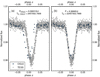 |
Fig. 1 Phased OGLE I-band and TESS light curves around the primary eclipse. Left panel: light curve phased according to the ephemeris from the OGLE catalog. Right panel: light curve phased according to the ephemeris we derive in this work by fitting the primary’s eclipses of the TESS light curve. |
3.1.2 RVs
To measure the RVs, we use a Markov chain Monte Carlo (MCMC) method combined with a least-square fitting method. In the MCMC method, the individual synthetic spectra of the primary and secondary (see Sect. 4.1) are shiftedby different RVs. The combined synthetic spectrum is then compared to the observation. Using a least-square likelihood function we estimate the quality of the used RVs. The MCMC method quickly explores a large parameter space of different RVs until it converges toward the true solution. In the vicinity of the true solution, the MCMC method calculates the probabilities of different combinations of the RVs. This yields the final probability distribution around the true solution. A more detailed explanation is given in Appendix A.
Because the final probability distribution obtained with the MCMC method is not necessarily a Gaussian, we quote the error as the 68% confidence interval. The PHOEBE code cannot handle asymmetric errors, and therefore we only use the larger margin of the probability distribution as it is the safer choice. The uncertainties are included in the eclipsing binary modeling as described in Sect. 3.1.3.
The primary dominates the emission and absorption lines. In order to avoid uncertainties due to the intrinsic variability of lines formedin the stellar wind, the RVs listed in Table 1 are the averaged values of the RVs obtained from selected individual lines. A more detailed list of the RVs obtained from the individual lines in the different optical spectra is given in Tables A.1 and A.2.
All the absorption lines that are associated with the secondary show a contribution from the primary. Furthermore, the depths of these absorption lines are at the level of the noise, which introduces additional uncertainties; these are reflectedin the larger error margins. Two selected optical spectra obtained at different phases are depicted in Fig. 3 to demonstrate how the spectral lines associated with the different binary components shift.
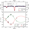 |
Fig. 2 Upper panel: phased OGLE I-band light curve of AzV 476 (blue dots) and the best fit obtained with the PHOEBE code (red line). Above the light curve, the spectral IDs of all used spectra (see Table 1) are indicated. Lower panel: observed (triangles) and fitted (solid lines) RV curves for the primary (green) and secondary (red). The fits of the light-curve fit and the RVs are consistently obtained by the PHOEBE code. |
3.1.3 Modeling with PHOEBE
The Physics of Eclipsing Binaries (PHOEBE) v.2.3 modeling software (Prša & Zwitter 2005; Prša et al. 2016; Horvat et al. 2018; Jones et al. 2020; Conroy et al. 2020) is employed to derive dynamic masses as well as to obtain measures of the stellar parameters independently from the spectroscopic model. The simultaneous fitting of the RV and light curve is done with the emcee sampler (Foreman-Mackey et al. 2013).
To reduce the parameter space, we fix the orbital period and the epoch of the primary eclipse to the values we derive from the TESS light curve; see Sect. 3.1.1. As we are using only one passband, the temperatures of the components cannot be obtained reliably. Therefore, the temperatures of the primary and secondary are fixed to the results from the spectral analysis (see Sect. 4.1), Teff, 1 = 42 kK and Teff, 2 = 32 kK, respectively.
The PHOEBE code assumes synchronous stellar rotation. The actual fast rotation of the secondary with v sin i = 425 km s−1 is therefore not consistently taken into account for modeling the secondary eclipse. Gravitational darkening is modeled by a power law with a coefficient of βgrav = 1, as recommended for radiative envelopes in the PHOEBE documentation3. Given the period of ~10 d, this renders gravitational darkening unimportant.
The atmospheres of both components are approximated by a blackbody. We compared the blackbody flux to the SED of our atmosphericmodel and find that it is a valid approximation for the I-band flux. We calculated the emergent flux distribution using our spectral models (see Sect. 4.1) and fitted different types of limb-darkening laws (e.g., Diaz-Cordoves & Gimenez 1992). We find that the limb-darkening law that best describes the primary and secondary is a quadratic approximation in the form of
![Mathematical equation: \begin{equation*}I(\mu)=I(1)\,[1-a_i\,(1-\mu)-b_i\,(1-\mu)^2],\end{equation*}](/articles/aa/full_html/2022/03/aa41738-21/aa41738-21-eq3.png) (3)
(3)
where μ = cosθ is the cosine of the directional angle θ, and ai and bi are the limb-darkening coefficients of each stellar component i. For the primary, the best fit is achieved with coefficients a1 = 0.2032 and b1 = 0.0275, while for the secondary a2 = 0.1668 and b2 = 0.0802 are required.
In a binary where both stellar components have large radii, on the order of ≳ 20% of their separation, and rather similar temperatures, the so-called “reflection effect” becomes important (Wilson 1990). This effect accounts for the irradiation of the surface by the other component (Prša 2011; Prša et al. 2016). As AzV 476 is a close binary with two hot O-stars, the reflection effect is modeled with two reflections. The effect of ellipsoidal variability due to tidal interaction, which induces periodic variations in the light curve, is important in close binary systems with orbital periods on the order of a few days (Mazeh 2008). However, as none of the binary components are close to filling their Roche lobe (see Table 4) and the mass ratio is not extreme (qorb = 0.89) this effect is expected to be negligible (Gomel et al. 2021).
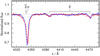 |
Fig. 3 X-shooter spectrum (ID 5 in Table 1) displayed in blue and one of the UVES spectra (ID 10 in Table 1) in red. The spectra are convolved with a Gaussian with an FWHM = 0.4 Å to reduce the noise and to make the RV shifts visible. The region containing Hγ, He I λ4387, and He I λ4471 lines is shown. In the spectrum shown by the red line, the primary’s spectrum is redshifted (see Hγ), while the secondary’s spectrum (broadened He I lines) is blueshifted. We note that the primary also partially contributes to the He I lines. |
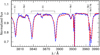 |
Fig. 4 Same as Fig. 3, but now for the region around the He I λ3819 and Hϵ lines. Most of the lines, including He I λ3926, are redshifted and associated with the primary, while the He I λ3819 line which isassociated with the secondary is blueshifted. |
Stellar parameters obtained from the RV and light curves by the PHOEBE code.
3.2 Resulting binary parameters
The best fitting model light curve and RV fit obtained with the PHOEBE code are shown in Fig. 2. The corresponding stellar parameters of both components are listed in Table 4 and the orbital parameters in Table 5. The orbital solution yields similar masses for both components, while the light curve fit reveals different Teff and L. This indicates that there was a prior mass-transfer phase that has stripped away most of the primary’s envelope, such that now has similar mass to its companion. From the light-curve fit, the fundamental stellar parameters –stellar radius and the surface gravity – are determined, giving us the opportunity to cross-check the spectral analysis. Furthermore, the PHOEBE code calculates the light ratio of the binary components in the observed band outside conjunctions, which is compared to the light ratio obtained from the spectroscopic analysis in Sect. 4.
Orbital parameters obtained from the RV and light curves by the PHOEBE code.
4 Spectral analysis
4.1 Method: Spectral modeling with PoWR
Synthetic spectra for both stellar components were calculated with the Potsdam Wolf–Rayet (PoWR) model atmosphere code (Gräfener et al. 2002; Hamann & Gräfener 2004). In the following, we briefly describe the code. For further details, we refer to Gräfener et al. (2002), Hamann & Gräfener (2003), Todt et al. (2015), and Sander et al. (2015).
The PoWR code models stellar atmospheres and winds permitting departures from local thermodynamic equilibrium (non-LTE). The code has been widely applied to hot stars at various metallicities (e.g., Hainich et al. 2014, 2015; Oskinova et al. 2011; Reindl et al. 2014; Shenar et al. 2015). The models are assumed to be spherically symmetric, stationary, and in radiative equilibrium. Equations of statistical equilibrium are solved in turn with the radiative transfer in the co-moving frame. Consistency is achieved iteratively using the “accelerated lambda operator” technique. This yields the population numbers within the photosphere and wind.
The emergent spectrum in the observer’s frame is calculated with the formal integral in which the Doppler velocity is split into the depth-dependent thermal velocity and a “microturbulence velocity” ζ(r). The microturbulence grows from its photospheric value ζph = 10 km s−1 linearly with the wind velocity up to 0.1v∞.
By comparison of the synthetic spectrum with the observations, it is possible to determine the main stellar parameters. In addition to the chemical composition, the main stellar parameters that specify the model atmosphere are the luminosity L, stellar temperature T*, surface gravity g*, wind mass-loss rate Ṁ, and the wind terminal wind velocity v∞. The stellar temperature is defined as the effective temperature referring to the stellar radius R* by the Stefan-Boltzmann equation  . The stellar radius is defined at the Rosseland mean optical depth of τ = 20. The differences between T* and the effective temperature Teff (referring to the radius where the optical depth τ = 2∕3) are negligibly small, as the winds of OB-type stars are optically thin.
In the subsonic regions of the stellar atmosphere, the velocity law is calculated such that the density, related by the equation of continuity, approaches the hydrostatic stratification. The hydrostatic equation consistently accounts for the radiation pressure (Sander et al. 2015). In the supersonic regions, it is assumed that the wind velocity field can be described by a so-called double β-law as was first introduced by Hillier & Miller (1999):
![Mathematical equation: \begin{equation*}\varv(r) = \varv_{\infty}\left[\left(1-f\right)\left(1-\dfrac{r_0}{r}\right)^{\beta_1}+f\,\left(1-\dfrac{r_1}{r}\right)^{\beta_2}\right].\end{equation*}](/articles/aa/full_html/2022/03/aa41738-21/aa41738-21-eq5.png) (4)
(4)
In this work, we assume β1 = 0.8, a typical valuefor O-stars, β2 = 4, and a contribution of f = 0.4 of the second β-term. r0 and r1 are close to the stellar radius R* and are determined such that the quasi-hydrostatic part and the wind are smoothly connected. This choice of the wind velocity law leads to better agreement between the Hα absorption line and the C IV P Cygni line profile than the classical β-law (Castor et al. 1975).
Inhomogeneities within the wind are accounted for as optically thin clumps (“microclumping”) which are specified by the “clumping factor” D, which describes by how much the density within the clumps is enhanced compared to a homogeneous wind with the same mass-loss rate (Hamann & Koesterke 1998b). In our analysis, we use a depth-dependent clumping which starts at the sonic point and increases outward until a clumping factor of D = 20 is reached at a radius of RD = 7 R* for the primary and at a radius RD = 10 R* for the secondary. The smaller radius at which the clumping factor is reached in the primary’s wind profile is needed to model the observed O V λ1371 line properly.
The PoWR model atmospheres used here account for detailed model atoms of H, He, C, N, O, Mg, Si, P, and S. The iron group elements Sc, Ti, V, Cr, Mn, Fe, Co, and Ni are combined to one generic element “G” with solar abundance ratios, and treated in a superlevel approach (Gräfener et al. 2002). The abundances of Si, Mg, and Fe are based on Hunter et al. (2007, their Table 17) and Trundle et al. (2007, their Table 9). For the remaining elements, we divide the solar abundances of Asplund et al. (2005, their Table 1) by seven to match the previously mentioned metallicity of the SMC. This yields the following mass fractions: XH = 0.73, XSi = 1.3 × 10⁻⁴, XMg = 9.9 × 10⁻⁵, XP = 8.32 × 10⁻⁷, XS = 4.42 × 10⁻⁵, and XG = 3.52 × 10⁻⁴. The CNO individual abundances of both stellar components are not fixed but derived from the analysis. The complement mass fraction to unity is XHe.
We determined the color excess EB-V and the luminosity L of the binary components by fitting the composite SED to photometry (top panel in Fig. 9). Reddening is modeled as a combined effect of the Galactic foreground, for which we adopt the reddening law of Seaton (1979) with EB-V = 0.03 mag, and the reddening law of Bouchet et al. (1985) for the SMC.
We use the iacob-broad tool (Simón-Díaz & Herrero 2014) in combination with the high S∕N X-shooter spectrum (S/N ~100) to determine the rotation rates of the primary and the secondary. The helium lines are potentially pressure broadened and thus are not optimally suited for rotation broadening measurements. Therefore, for the primary, we use the few metal lines that are visible in the optical spectrum, namely the N IV λ3478 and the O IV λ3403 absorption lines and the N IV λ4058 emission line. We determine a projected rotation rate of v1 sini = 140 km s−1 for the primary. The secondary only contributes to the He I lines. Fitting the He I λ4387 and He I λ4471 absorption lines – in which the contribution of the primary is smallest – yields a rotation rate of v2 sini = 425 km s−1 for the secondary.
Previously, Penny & Gies (2009) determined the projected rotational velocity of the primary to v1 sini = 65 km s−1 using a cross-correlation of the FUSE spectrum in the far-UV with a template spectrum. We calculate tailored spectral models with the respective projected rotational velocities and find that also the FUSE spectrum is better reproduced when using v1 sini = 140 km s−1 (see Fig. 6). We assume that the template spectrum used in Penny & Gies (2009) might not have been perfectly calibrated for our target and that the binary nature leads to additional uncertainties.
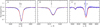 |
Fig. 5 Selected regions of the X-shooter spectrum (ID 5 in Table 1) compared to different synthetic spectra. The observed spectrum, corrected for the velocity of the SMC and the barycentric motion, is shown as a solid blue line. The red dotted line is our best-fitting model which consists of the primary with Teff, 1 = 42 kK and log g*, 1 = 3.7 and the secondary with Teff, 2 = 32 kK and log g*, 1 = 4.0. The gray solid line is again a combined synthetic spectrum of the primary and secondary, but this time the surface gravity of the primary has been reduced to log g*, 1= 3.6 (and the temperature and mass-loss rate are slightly adjusted so that the spectrum matches the observations) while the parameters of the secondary are kept fixed. The line identification marks correspond to the wavelengths in the rest frame. Panel a shows the Hγ line, in which the red wing is dominated by the primary and the blue wing by the secondary. Panel b shows the He II λ5412 absorption line, which is dominated by the primary and is sensitive to surface gravity. Panel c shows the region of He II λ6528 and Hα. While the Hα wings are only barely affected by the change in logg*, 1, the He II λ6528 line is more sensitive to it. |
4.2 Resulting spectroscopic parameters
4.2.1 Temperature and surface gravity of the primary
AzV 476 was previously classified as O2–3 V plus a somewhat later O-type companion. This implies that nitrogen lines are expected in absorption and emission in the primary spectrum, while He I absorption lines should be present in the secondary spectrum.
Indeed, we find that the N IV λ4057 (hereafter N IV) emission line, the N IV absorption lines at λλ 3463 Å, 3478 Å, 3483 Å, and 3485 Å, and the He II λ6528 absorption can be entirely assigned to the primary. We observe only marginal N III λλ4634, 4640 (hereafter N III) emission and N V λλ4603, 4619 (hereafter N V) absorption; see Fig. B.1. Thus, the optical spectrum shows nitrogen only as N IV, while N III as well as N V are virtuallyabsent. This restricts the temperature of the primary to a narrow range (Rivero González et al. 2012). We also find that the O IV multiplets around 3400 Å are purely associated with the primary. Because these lines are highly contaminated by ISM absorption lines of Ti II λ3385 and Co I λ3414, they are only used as a crosscheck of the oxygen abundance applied in our spectral model. A more detailed description of this line complex is given in Appendix B.2.
The secondary does not contribute noticeably to these weak metal lines. However, the secondary strongly dominates the He I absorption lines at λλ I3819 Å, 4387 Å, and 4471 Å, indicating a lower effective temperature. The primary star also contributes to these lines, giving additional constraints on the temperature of the primary.
The surface gravity g*, 1 of the primary is determined by fitting the wings of the Balmer lines using those UVES spectra with the least wavy patterns and highest RV shifts as well as the X-shooter spectrum, which has a higher S∕N. Because both stars contribute to the Balmer lines, the He II λ5412 absorption line that is mostly originating from the primary and also sensitive to changes in surface gravity is used. Unfortunately, this line is only contained in the X-shooter spectrum. Surface gravity affects the density structure and therefore the ionization balance of, for example, nitrogen and helium. As the temperature is adjusted such that the nitrogen lines are reproduced, changes in the surface gravity will not only affect the wings of the He II lines but also change the depth of the He II absorption lines. This gives the opportunity to use the He II λ6528 absorption line in the UVES spectra as second criterion for the surface gravity estimate in the primary.
We tested different temperature values in the range Teff, 1 = 39 kK−50 kK and surface gravities in the range log(g*, 1∕(cm s−2)) = 3.5−4.1 and found that a temperature of Teff, 1 = 42 ± 3 kK and a surface gravity of log(g*, 1∕(cm s−2)) = 3.7 ± 0.2 are most suitable for reproducing the primary’s spectrum. The given error margins take into account that the measurements of temperature and surface gravity are not independent.
Different regions of the X-shooter spectrum that are used to determine the surface gravity are shown in Fig. 5. The accuracy in surface gravity highly depends on the calibration of the spectrum. One can see that Hγ and He II λ5412 line fits show preference to a surface gravity for the primary of log(g*, 1∕(cm s−2)) = 3.7, while Hα and He II λ6528 indicate that log(g*, 1∕(cm s−2)) = 3.6 might be more suitable. However, from fitting the UVES data with the highest RV shifts we find that a surface gravity for the primary of log(g*, 1∕(cm s−2)) = 3.7 yields the best fit.
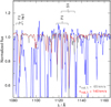 |
Fig. 6 Part of the observed FUSE spectrum (ID 1 in Table 1) covering the wavelength range of the LiF2 channel – the same as used by Penny & Gies (2009) to determine the projected rotational velocity. The observed spectrum, corrected for the velocity of the SMC, is shown as a solid blue line. The red dotted line is our best-fitting model with the primary’s projected rotational velocity v1 sin i = 140 km s−1. The gray solid line is another model where the primary’s projected rotational velocity is reduced to v1 sin i = 140 km s−1. The line identification marks correspond to the wavelengths in the rest frame. |
4.2.2 Temperature and surface gravity of the secondary
It is more difficult to determine the temperature of the secondary, as only a few He I lines are associated with the secondary and all these line have a contribution from the primary. However, from the spectra with the highest RV shifts (e.g., UVES spectrum with ID 10), we find that the secondary does not contribute to the He II λ4200 line, and therefore we have an additional constraint that can be used as an upper limit on the temperature of the secondary. In addition to the limited number of lines that are associated with the secondary, the ionization balance that changes depending on the surface gravity introduces another uncertainty in our temperature estimation.
Therefore, we first adjust g*, 2 of the secondary such that the wings of the Balmer lines are well reproduced while keeping the surface gravity and temperature of the primary fixed. As in the case of the primary, in order to distinguish the contributions of the binary components to the Balmer wings, we employ the UVES spectra in the phase with the largest RV shifts. This gives additional information and a surface gravity of log (g*, 2∕(cm s−2)) = 4.0 can be determined. Finally, the temperature of the secondary is adjusted such that the He I absorption lines at λλ 3819 Å, 4387 Å, and 4471 Å match the observation. Following this procedure, the spectrum of the secondary is best reproduced with a temperature of Teff, 2 = 32 kK. This method is accurate to ΔTeff, 2 = ±4 kK in temperature and Δlog(g*, 2) = ±0.2 for the surface gravity. The obtained values of the surface gravity of the primary and the secondary are in agreement with those obtained from the orbital analysis (see Sect. 3).
4.2.3 Luminosity
To estimate the light ratio, the luminosities of both stars are adjusted such that the shapes of the optical He II lines match the observations. This is an iterative process done simultaneously with the temperature and surface gravity estimate. The total luminosity of the system is calibrated such that the calculated visual magnitude of the synthetic flux matches the observed one. This results in luminosities of log(L1∕L⊙) = 5.65 for the primary and log(L2∕L⊙) = 4.75 for the secondary. This estimate is sensitive to synthetic spectra, light ratio, and distance modulus. Therefore, we estimate that our measurements of the luminosity of each stellar component are accurate to Δ log(L∕L⊙) = ±0.2.
Taking these uncertainties into account, the model flux ratio in the OGLE I-band yields f2 ∕f1 = 0.26 ± 0.1 which is in agreement with the flux ratio derived using PHOEBE f2∕f1 = 0.31 ± 0.05 (see Sect. 3).
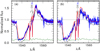 |
Fig. 7 Observed (blue) and synthetic (red) C IV resonance doublet of our final model. The individual primary and secondary spectra are shown as dotted black and green lines, respectively. The sharp interstellar absorptions arise in the Galactic foreground and in the SMC, and are also modeled with their respective RV shifts. (a) COS observation (ID 2 in Table 1) (b) STIS observation (ID 3 in Table 1). |
4.2.4 Mass-loss rates
After determining the temperatures, surface gravities, and luminosities of both binary components, we proceed to measuring the properties of their stellar winds. The Hα line in the optical as well as the C IV resonance line in the UV are used as the main diagnostic tools for measuring the mass-loss rate of the primary. In addition, we also pay attention to the appearance of the optical He I λ4686 and the UV He II λ1640 line; see Fig.B.3. When calibrating the mass-loss rate of the primary, the best fit is archived with a mass-loss rate of log (Ṁ1∕(M⊙ yr−1)) = −6.1 ± 0.2 and a terminal wind velocity of v∞, 1 = 2500 km s−1.
We have two spectra covering the C IV resonance line at different phases, the COS and the STIS spectrum (ID 2 and 3 in Table 1), depicted in Fig. 7. The C IV P Cygni line profile in both spectra does not show any direct indications for the contribution from the secondary such as a double emission peak or a step in the absorption trough. The C IV resonance line in the STIS spectrum shows slightly weaker emission, which is most likely due to the sensitivity of the different instruments or weak wind variability. We use the bottom part of the P Cygni profile of C IV resonance line to confirm the continuum contribution of the secondary in the UV and therefore the used light ratio (L2 ∕L1).
Apparently the secondary does not contribute to the wind lines. Its mass-loss rate can therefore only be limited to log (Ṁ2∕(M⊙ yr−1)) ≤−8.8 ± 0.5. For higher mass-loss rates, we find that the secondary would noticeably contribute to the C IV resonance line in the UV. Due to the lack of indications of the secondary’s wind we adopt the terminal velocity of the primary, v∞, 2 = 2500 km s−1.
4.2.5 CNO surface abundances
As already explained in Sect. 4.1, the abundances of hydrogen and the iron group elements are fixed, while the CNO abundances of each stellar component are adjusted during spectral modeling. The nitrogen abundance is adjusted to find good agreement with the optical N IV absorption lines at wavelengths 3463 Å, 3478 Å, and 3483 Å, and the N IV λ4057 and N IV λλ7103−7129 emission lines, as well as the UV N V λλ1238, 1242 resonance doublet. The best agreement is achieved with a nitrogen mass fraction of 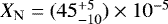 . The nitrogen lines seen in the optical are displayed in Fig. 8.
A carbon abundance of 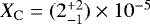 reproduces the optical C IV λλ5801, 5812 lines best while maintaining the fit of the C IV resonance doublet, at least for mass-loss rates that do not conflict with other wind features. For lower abundances, the latter is no longer saturated. The oxygen abundance of the primary is calibrated with the oxygen absorption lines in the UV and the optical O IV multiplets around 3400 Å, resulting in
  .
.
There are no strong CNO lines in the secondary spectrum, and therefore we adopt initial CNO abundances scaled to the metallicity of the SMC (ZSMC = 1∕7 Z⊙). Alternatively, one could assume that the surface abundances in the secondary are close to those in the primary as the accreted material is polluting the surface of the secondary. We explored both assumptions but could not find diagnostic lines that would allow us to pin down the composition of the atmosphere and wind of the secondary. We are only able to fix upper limits for the CNO abundances such that these elements would not produce features that are inconsistent with the observations: XN ≲ 50 × 10−5, XC ≲ 21 × 10−5 and XO ≲ 110 × 10−5.
4.2.6 Required X-ray flux
Similar to other O-type stars, AzV 476 shows a notoriously strong P Cygni profile in the O VI λλ1032, 1038 resonance doublet. However, wind models do not predict a sufficient population of this high ion without the inclusion of additional physical processes. This phenomenon, termed “super-ionization”, was described by Cassinelli & Olson (1979) and interpreted as evidence for the presence of an X-ray field in stellar atmospheres.
In order to model the O VI doublet in the observed spectrum of AzV 476, we add a hot plasma component. The X-ray-emitting plasma has an adopted temperature of TX = 3 MK and is distributed throughout the wind outside a radius of RX = 1.1 R*. Its constant filling factor is a free parameter; the best reproduction of the observation is achieved for a model with an emergent X-ray luminosity of log LX = 31.4erg s−1.
Current X-ray telescopes are not sensitive enough to detect individual O stars in the SMC. Our final model predicts an X-ray flux at earth of 1.4 × 10⁻¹⁷ erg s−1 cm−2 Å−1 integrated over the X-ray band (≈ 6–60Å). The region on the sky where AzV 476 is located was observed by both XMM-Newton and Chandra X-ray observatories. However, despite the detection of AzV 476 in the UV by the XMM-Newton optical monitor, the star is not detected in X-rays. Hence, we set the upper limit on its X-ray flux at the median flux of detected sources in the XMMSSC – XMM-Newton Serendipitous Source Catalog (4XMM-DR10 Version); this is 5 × 10⁻¹⁵ erg s−1 cm−2 Å−1, which is far from being sufficiently sensitive for our predicted source.
The O VI resonance doublet is not the only feature that is sensitive to X-rays. Other ions which might be populated by Auger ionization are N V and N IV. We find that the N V λλ1242, 1238 resonance doublet in our model is not significantly affected by the applied X-ray field, while the N IV λλ1718, 1721 doublet is very sensitive. However, in the region around the N IV λλ1718, 1721 doublet, theobservations are very noisy and can be explained by the model with X-rays as well as without.
The composed model spectrum as well as the individual spectra are shown in Figs. 5–10. A summary of the stellar parameters including the abundances is given in Table 6.
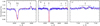 |
Fig. 8 Observed X-shooter spectrum (ID 5 in Table 1) and synthetic spectra of selected regions that show nitrogen emission lines. The observed spectrum is shown as a solid blue line, while the dotted red line is our best-fitting model. The observed spectrum is corrected for the velocity of the SMC and the barycentric motion. The line identification marks correspond to the wavelengths in the rest frame. Panel a shows the area around the N IV λ4057. Panel b shows the region of N III λλ4511−4523, N V λλ4604, 4620, and N III λλ4634, 4641. The N III and N V lines are not observable in the spectrum. Panel c shows the region of the N IV λλ7103−7129 complex. |
Summary of the stellar parameters of both stellar components obtained from the different methods.
4.2.7 Spectroscopic stellar masses
The spectroscopic masses derived from our analysis are  for the primary and
  for the secondary. The spectroscopic masses, although a factor of 1.5 higher than the orbital masses, agree with these latter within their respective uncertainties. The large error margins on the spectroscopic masses arise mainly from the large uncertainties on surface gravity and luminosity (e.g., Fig. 5). The spectroscopic mass ratio is qspec = 0.7 which is smaller than the one obtained from the orbital analysis.
It appears that the spectroscopically derived masses and luminosities are shifted systematically to higher values compared to the results of the orbital analysis. We discuss this in more detail in Sect. 6.1.
Nevertheless, a mass ratio close to unity, while the two stars in a close binary have different spectral types, strongly suggests mass transfer in the past. From our binary evolutionary models (Sect. 5), we expect that mass transfer removed most of the hydrogen-rich envelope from the primary. We calculated model spectra with strongly depleted surface hydrogen (XH = 0.2 and 0.5). However, these models yield poorer spectral fits as the helium lines become too deep. Still, moderate hydrogen depletion and helium enrichment cannot fully be excluded.
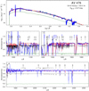 |
Fig. 9 Spectral fit for AzV 476. Top panel: SED. Flux-calibrated observations (blue lines) are the FUSE (1), COS (2), STIS (4), and X-shooter (5) spectra as listed in Table 1. The light blue squares are the photometric UBVRIJHK data as listed in Table 2. The model SED composed of both stellar components is shown as a dashed red line, while the individual SEDs of the primary and the secondary are shown as dotted black and green lines, respectively.Lower panels: normalized FUSE (1), COS (2), and STIS (4) spectra. The number in the upper left corner corresponds to the ID given to a specific spectrum as listed in Table 1. The line styles are the same as in the top panel. The synthetic spectra are calculated with the model parameters compiled in Table 6 (“Spectroscopy” columns). |
4.3 Revisiting the spectral classification
AzV 476 was previously classified on the basis of the appearance of its optical spectrum. However, during our spectroscopic analysis, we found that most of the classification lines are blended by the companion. Hence, including the additional information from our spectroscopic models and the available UV data allows us to reconsider the spectral classification.
We used the Marxist Ghost Buster (MGB) spectral classification code (Maíz Apellániz et al. 2012; Maíz Apellániz 2019). MGB compares observed spectra with the criteria of Walborn et al. (2000, 2002, 2014) and Sota et al. (2011, 2014) while allowing the presence of two components by iteratively adjusting the spectral types, light ratio, RVs, and rotational indices. This approach poses two problems. First, the low metallicity of the SMC leads to weaker nitrogen lines compared to stars with similar type in the MW and LMC. Second, only the X-shooter spectrum is covering the whole wavelength range of 3900 Å−5100 Å which is needed for a spectral classification. In addition we consider those UVES spectra with the highest RV shifts in order to better separate the individual binary components.
Therefore, we are forced to use the X-shooter spectrum first and then consider the UVES spectra with the highest RV shifts that cover the range from 3300 to 4500 Å.
The MGB code provides the spectral type O4 IV((f)) for the primary. The main reason for the slightly later subtype assigned to the primary is its contribution to the He I λ4471 line. The suffix “((f))” is assigned because of the barely detectable N III λλ4634, 4641 lines (see Fig. B.1). Regarding the secondary, the absence of the He II λ4200 line suggests the latest O subtype, O9.5: Vn. The suffix “n” refers to the high rotational broadening of the lines of the secondary.
The MGB classification code only considers the optical range of the spectrum. If one inspects the UV spectrum, which mostly originates from the primary, and compares it to the N V and C IV UV wind-profile templates with those presented in Walborn et al. (2000), one might prefer a luminosity class “III” for the primary. The difference in the optical spectral appearance is explainable by the high L/M ratio which leads to very strong mass loss and thus to exceptionally strong wind lines in the UV. In light of these circumstances and the unusual chemical composition, we add the suffix “p” for this peculiar object. In the end, we therefore classify the system as O4 IV-III((f))p + O9.5: Vn.
Following the work of Weidner & Vink (2010), an isolated star with spectral type O4 III is expected to have a stellar mass of about  which is more than twice as high as that which we derive using two different methods (Sects. 3and 4.1). For the O9.5: V secondary, the mass expected from the spectral type would be
  which agrees within uncertainties with the findings of the orbital and spectroscopic analysis.
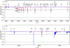 |
Fig. 10 Same as Fig. 9, but now the normalized optical X-shooter spectra (ID 5 in Table 1) are shown. |
5 Stellar evolution modeling
From orbital and spectroscopic analysis, we find that the mass ratio is close to unity, although the two binary components have distinctly different luminosities, effective temperatures, and rotation rates: the secondary is a fast rotator while the rotation of the primary is only moderate. These facts strongly indicate that the system has already undergone mass transfer.
5.1 Single-star models
As a first approach, we investigate whether the stellar parameters of the individual components can be reproduced by single-star evolutionarymodels. For this purpose, we employ the Bayesian statistic tool “The BONN Stellar Astrophysics Interface” (BONNSAI4), (Schneider et al. 2014) in combination with the BONN-SMC tracks (Brott et al. 2011). To find a suitable model, we request the tool to match the current luminosity, effective temperature, rotation rate, and orbital mass of the two stars. Indeed, we find that the fast-rotating secondary can be partially explained by a single-star track. With respect to the primary, the BONNSAI tool cannot find any track that would explain its current low mass. Only when ignoring the mass constraint are we able to find a suitable track that reproduces the remaining stellar parameters. In that case, the predicted ages of the primary and secondary differ by a factor of two. This finding confirms our suggestion that the system has already undergone mass transfer. The best-fitting stellar parameters obtained with the BONNSAI tool – applicable only for single stars – are listed in Table 6.
5.2 Binary evolutionary models
The binary models are calculated with MESA v. 10398. To mimic the BONN-SMC tracks we adjusted MESA in a similar way to that described by Marchant (2016). We follow most of the physical assumptions from the BONN-SMC models (e.g., overshooting, thermohaline mixing, etc.) and adopt them from Marchant (2016) with two exceptions. In our models, we use a more efficient semi-convection with αsc = 10 and calculate the mass transfer according to the “Kolb” scheme (Kolb & Ritter 1990), as it allows us to include the eccentricity enhancement mechanism meaning that the evolution of the eccentricity can be modeled properly.
We want to emphasize that our goal is to check whether binary evolutionary models can explain the stellar parameters of AzV 476 and especially its masses. Therefore, we only explore a narrow parameter space and compute a small set of models with initial primary masses in the range of Mini, 1 = (25−38) M⊙ and secondary masses Mini, 2 = (10−25) M⊙, orbital periods in the range of Pini = 8 d25 d and initial eccentricities eini = 0.0−0.4. The initial parameters are adjusted such that at some later stage the model binary has properties similar to AzV 476. We assume that the stellar components initially rotate with vrot = 0.1 vcrit ≈ 65 km s−1. These values are chosen arbitrarily but as we are dealing with a close binary, the tidal forces nevertheless lead to a tidal synchronization. Further important assumptions are as follows:
Our models include the effect of inflation, which appears inside a stellar envelope when the local Eddington limit is reached and exceeded, leading to a convective region and a density inversion (Sanyal et al. 2015).
The stellar wind prescription is inspired by the work of Brott et al. (2011). The winds of hot H-rich stars are described according to the Vink et al. (2001) recipe. For stars with effective temperatures below the bi-stability jump, where mass-loss rates abruptly increase (see Vink et al. 2001), we use the maximum Ṁ from either Vink et al. (2001) or Nieuwenhuijzen & de Jager (1990). WR mass-loss rates are according to Shenar et al. (2019) but are assumed to scale with metallicity as Ṁ ∝ Z1.2 as recommended by Hainich et al. (2017). In the transition phase from a hot H-rich star (XH ≥ 0.7) to the WR stage (XH ≤ 0.4), the mass-loss rate is interpolated between the prescriptions of Vink et al. (2001) and Shenar et al. (2019).
Rotational mixing is modeled as a diffusive process including the effects of dynamical and secular shear instabilities, the Goldreich-Schubert-Fricke instability, and Eddington–Sweet circulations (Heger et al. 2000). In addition to the angular momentum transport by rotation, the transport via magnetic fields from the Tayler–Spruit dynamo (Spruit 2002) is also included.
Convection is described according to the Ledoux criterion and the mixing length theory (Böhm-Vitense 1958) with a mixing length parameter of αmlt = l∕HP = 1.5. For hydrogen burning cores, a steep overshooting is used such that the convective core is extended by 0.335HP (Brott et al. 2011) where HP is the pressurescale height at the boundary of the convective core. Thermohaline mixing is included with an efficiency parameter of αth = 1 (Kippenhahn et al. 1980), as well as semiconvection with an efficiency parameter of αsc = 10 (Langer et al. 1983).
Mass transfer in a binary is modeled using the “Kolb” scheme (Kolb & Ritter 1990). This allows us to use the Soker eccentricity enhancement (Soker 2000), which assumes phase-dependent mass loss and calculates the change in eccentricity due to the mass that is lost from the system, and the mass that is accreted by the companion. Tidal circularisation is taken into account throughout the entire evolution of the system.
The remaining mass collapses into a compact object – represented by a point mass – when helium is depleted in the stellar core. This simplification avoids numerical problems in the latest burning stages and the unknowns that come with a supernova explosion and a possible kick.
As the luminosities obtained from the spectroscopic and orbital analysis differ to some extent, we put additional focus on reproducing the orbital masses, which are our most reliable estimate. The best agreement with the empirically derived parameters is found for a system with initial masses Mini, 1 = 33 M⊙ and Mini, 2 = 17.5 M⊙, initial orbital period Pini = 12.4 d, and initial eccentricity eini = 0.14. The model closest to the current stellar parameters gives similar masses for the primary and secondary: Mevol, 1 = 17.8 M⊙ and Mevol, 2 = 18.2 M⊙. The remaining stellar parameters of our favorite models are listed in Table 6.
The Hertzsprung-Russell diagram (HRD) displaying the best fitting stellar evolutionary tracks for both binarycomponents is illustrated in Fig. 11. The binary evolution model is able to reproduce almost all empirically derived stellar parameters including the current orbital period (Pmodel = 9.3 d) and the eccentricity of the system (emodel = 0.25). However, the evolutionary models over-predict the rotation rate of the secondary and the surface abundances of the primary; see Table 6. We calculated PoWR atmosphere models with the best fitting parameters obtained with our MESA models. Thesynthetic spectra are shown in Fig. B.4.
A more fine-tuned model would likely solve some of these problems. For example, we did not include the initial rotation as a free parameter. This might solve the faster rotation of the primary; however, the secondary would still be expected to be rotating too fast as it spins up to criticality during mass transfer. According to our favorite evolutionary model, the primary in AzV 476 is currently evolving towards the helium zero age MS (ZAMS) and will possibly spend the rest of its life as a hot helium or WR-type star.
6 Discussion
6.1 Comparison of the orbital, spectroscopic, and evolutionary mass estimates
The orbital masses and the masses predicted by the binary evolutionary models agree well within their error margins and deviate only by 10%. On the other hand, the spectroscopic mass and luminosity of both components appear to be higher by a factor of 1.5 compared to the orbital solutions. The question therefore arises as to whether the discrepancy between the orbital and spectroscopic solutions is significant.
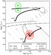 |
Fig. 11 HRD showing the positions of each binary component according to the spectroscopic and orbital analysis, and the best fitting binary evolutionary tracks. The results of the spectroscopic analysis are shown as triangles and the orbital analysis as upside-down triangles. The positions of the primary and secondary are marked in green and red, respectively. The shaded areas indicate the respective error-ellipses. Evolutionary tracks (solid lines) of both binary componentsare according to the best fitting binary model calculated with MESA (see Sect. 5.2). The tracks are labeled by their initial masses. The black dots on the tracks correspond to equidistant time-steps of 0.1 Myr to emphasize the most probable observable phases. The light blue dots mark the best-fitting model. |
6.1.1 Orbital versus spectroscopic mass
The simplest way to resolve this discrepancy is to assume that the distance to the system is lower than the canonical SMC distance of (d = 55 kpc). As the luminosity depends on the assumed distance as L ∝ d−2, the radius (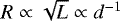 ) and the spectroscopic mass also depend on distance (Mspec ∝ R2 ∝ L ∝ d−2). The SMC galaxy is extended, and the distances to its various structural parts are not well established. Tatton et al. (2021) suggest that young structures, such as the NGC 456 cluster, are not well represented by the intermediate age stellar populations, which are usually used for distance estimates. Instead, young clusters might be located in front of these latter. This is in agreement with the argumentation by Hammer et al. (2015), who showed that the interactions between the LMC and SMC could lead to multiple tidal and ram-pressure stripped structures, which spatially separate young star-forming regions from older stellar populations.
In order to bring the spectroscopic and orbital parameters of AzV 476 into accordance, the system needs to be shifted to a distance of 49 kpc. The resulting spectroscopic masses are then Mshift, 1 ≈ 23 M⊙ and Mshift, 2 ≈ 18 M⊙. However, d = 49 kpc would imply that our target is located at the same distance as the LMC.
The LMC has higher metallcity (ZLMC = 1∕2 Z⊙) than the SMC (ZSMC = 1∕7 Z⊙), and therefore we speculate that stars formed in the interaction regions may have higher metallicity than the SMC. To test this, we increased the metallicity content of our spectroscopic models to the LMC metallicity while keeping the remaining stellar parameters unchanged. We find that the lines in the iron forest, especially in the far-UV, are too deep compared to the observations. Therefore, it cannot be confirmed that our target has LMC metallicity, but at the same time this does not provide additional constraints on its distance.
Another option we need to consider is the possibility of a third light contribution. AzV 476 is located in a very crowded region. Therefore, it is possible that the observed light is contaminated by a nearby object and hence the true luminosity (and mass) is lower. We inspected the HST acquisition image of our target and find no other nearby UV-bright stars. Alternatively our target could be a multiple system rather than a binary. If there were a third component, it would need to be of similar luminosity to the secondary in order to have an impact on our analysis. However, we do not see any indications of a third component in our spectra.
A third option is that the surface gravities determined from the spectral analysis are overestimated. The accuracy of the spectroscopic mass strongly depends on surface gravity, log g, which is mainly determined from fitting the pressure-broadened line wings. Such estimates suffer from limited S/N ratio in the spectra. In cases where the Balmer lines include contributions from both components, further uncertainties are induced. As explained in Sect. 4.2 and shown in Fig. 5, the He II lines help to improve the estimates, but still do not allow us to pin point log g for each component separately. This leaves room for various combinations of log g able to reproduce the Balmer lines and is reflected in the large uncertainties of the spectroscopic masses.
6.1.2 Orbital versus evolutionary mass
The evolutionary modeling yields a slightly lower mass for the primary than the spectroscopic and orbital analyses. As can be seen in Table 6, the evolutionary mass is 2 M⊙ lower than the orbital one.
For a given initial mass, the main parameter defining how much mass is lost during mass transfer by the primary is the initial binary orbital period. As a rule of thumb, the longer the initial orbital period, the less mass is removed from the donor star (Marchant 2016). However, several effects (e.g., eccentricity) influence the response of the orbit to mass transfer. For instance, an eccentric orbit leads to phase-dependent mass transfer, which potentially increases the eccentricity and widens the orbit. Thus, the donor can expand more, and less mass is removed via Roche-lobe overflow (Soker 2000; Vos et al. 2015).
The amount of mass lost during mass transfer is also reduced when the radial expansion of the star is minimized such that the star can stay underneath the Roche lobe. The radial expansion is affected by the mixing processes. For instance, a star with more efficient semi-convective mixing is expected to be more compact (e.g., Klencki et al. 2020; Gilkis et al. 2021). We computed a binary evolutionary model with a less efficient semi-convection of αsc = 1 and find that the post-mass-transfer (after detachment) mass of the primary is lowered by 1 M⊙. This is only one example and there are a handful of other processes that impact the mixing efficiency, energy transport, and the expansion of the envelope.
One more process that affects the radial expansion is the mass-loss rate which is described by the adopted mass-loss recipe (see Sect. 5). Over- or underestimating the mass-loss rate influences stellar evolution before, during, and after mass transfer. Interestingly, we find approximate agreement between the empirically derived mass-loss rate of the primary and the prediction of the wind recipe (see Sect. 6.2.1).
The evolutionary mass of a star after mass transfer is sensitive to various assumptions. Therefore, a difference of 2 M⊙ between evolutionary and orbital mass appears to be within the range of the evolutionary model uncertainties. While a more fine-tuned binary evolutionary model is beyond the scope of this paper, our modeling confirms that the orbital masses of AzV 476 are well explained by a post-mass-transfer binary evolutionary model. Therefore, this unique system is a useful benchmark for improving the understanding of mass transfer and mixing processes in close massive binaries. We conclude that the orbital, spectroscopic, and evolutionary mass estimates agree within their uncertainties.
6.2 The empirical mass-loss rate
Stellar evolution depends on the mass-loss rate. Stellar evolution models rely on recipes that are only valid for a given evolutionary phase. In transition-phases one typically interpolates between corresponding mass-loss recipes (e.g., Sect. 5). In the following, we compare the mass-loss rates we empirically derive from spectroscopy with other estimates as well as with the various recipes.
In this work, the mass-loss rates are primarily derived from resonance lines in the UV and the Hα line while taking into account the morphology of the He II λ1640 and He II λ4686 lines. The winds of all hot stars are clumpy (e.g., Hamann et al. 2008) which enhances the emission lines fed by recombination cascades (e.g., Hamann & Koesterke 1998a) such as the Hα line. Resonance lines in the UV are mostly formed by line scattering, a process that scales linearly with density and is thus independent from microclumping. Considering both Hα and the resonance lines allows us to constrain the clumping factor D and the mass-loss rate Ṁ consistently.
6.2.1 The primary
The spectroscopically derived mass-loss rate of the primary is log (Ṁ∕(M⊙ yr−1)) = −6.1 ± 0.2. Massa et al. (2017) derive a mass-loss rate of  from the IR excess. However, the clumping effects were not included in their analysis. As the IR excess originates from free-free emission, it scales with
  . Correcting the mass-loss rate with a clumping factor of D = 20, as assumed in our spectroscopic models, yields
  , which is in agreement with the optical and UV analyses.
In the massive star evolutionary models, the terminal wind velocity is prescribed as v∞ ∕vesc = 2.6 and the mass-loss rates of OB stars are prescribed according to the Vink et al. (2001) recipe. Using the stellar parameters obtained with spectroscopic analysis (see Table 6) and the prescribed v∞ = 1911 km s−1, the “Vink’s recipe” yields log(Ṁ∕(M⊙ yr−1)) = −6.1. Alternatively, applying the actual wind velocity measured from the UV spectra, v∞ = 2500 km s−1, the theoretical prediction changes to log(Ṁ∕(M⊙ yr−1)) = −6.2, which is in agreement with our empirical result within the uncertainties.
However, the primary’s current mass-loss rate adopted in our favored binary evolutionary model (log (Ṁ∕(M⊙ yr−1)) = −6.4) is lower. This is mainly caused by the interpolation between the mass-loss rate prescriptions for OB stars by Vink et al. (2001) and for WR stars by Shenar et al. (2019) which is employed when the surface hydrogen mass-fraction of the primary’s evolutionary model already dropped below XH < 0.7. Additionally, the stellar parameters (e.g., mass and luminosity) that enter the different mass-loss recipes employed by the evolutionary code are slightly different than those obtained from our spectral analysis.
Based on dynamically consistent Monte Carlo wind models, Vink & Sander (2021) suggest an updated scaling of metallicity for their mass-loss rates. This scaling yields higher mass-loss rates of log (Ṁ∕(M⊙ yr−1)) = −5.7, or, using the measured v∞ = 2500 km s−1, log (Ṁ∕(M⊙ yr−1)) = −5.9. Correcting in a simple way the former theoretical mass-loss rate for clumping results in log (Ṁ∕(M⊙ yr−1)) = −6.4, which is somewhat lower than our empirical measurement.
The spectroscopic measurements of mass-loss rates of O-dwarfs in the SMC deliver useful empiric prescriptions (e.g., Bouret et al. 2003; Ramachandran et al. 2019). According to Ramachandran et al. (2019, see their Fig. 15), the mass-loss rate of the primary star in AzV 476 would be only log (Ṁ∕(M⊙ yr−1)) = −7.4, which is much lower than obtained from our analysis. We explain this discrepancy by the advanced evolutionary status: the primary has already a substantially reduced mass due to its close-binary evolution, leading to a high L∕M ratio. This precludes the comparison with the recipes which use the mass–luminosity relations for single stars.
6.2.2 The secondary
There are no indications of wind lines of the secondary in the observed spectra. Therefore, we can only set an upper limit on the mass-loss rate log (Ṁ∕(M⊙ yr−1)) ≤−8.8 ± 0.5. The Vink et al. (2001) recipe predicts a higher value of log(Ṁ∕(M⊙ yr−1)) = −8.2. Correcting for clumping with D = 20 yields log(Ṁ∕(M⊙ yr−1)) = −8.8 which is in agreement with the empirical result.
According to Vink & Sander (2021), the predicted mass-loss rate of the secondary is log (Ṁ∕(M⊙ yr−1)) = −7.8; correcting it for clumping yields log(Ṁ∕(M⊙ yr−1)) = −8.4, which is higher than the empirical upper limit. The empirical relation of Ramachandran et al. (2019, their figure 15) suggests log (Ṁ∕(M⊙ yr−1)) = −8.6 ± 0.2, which is somewhat higher than our result but consistent with its error margins.
As can be seen in Table 6, the mass-loss rate used in the binary evolution calculation is higher than predicted by the recipes as well as empirically measured. This is because in the MESA models, the mass-loss rate of a star rotating close to critical is enhanced compared to slowly rotating stars (Paxton et al. 2013). The synthetic spectrum calculated with the parameters obtained by the binary evolutionary models displayed inFig. B.4 shows strong P Cygni profiles in the spectrum of the secondary (e.g., Si IV λλ1393.8, 1402.8) that are notobserved. We conclude that the mass loss of the secondary is not rotationally enhanced above the observed limit.
6.3 Comparison of the stellar parameters as predicted by MESA evolutionary tracks versus derived spectroscopically
In this work, AzV 476 is studied using two different approaches. (1) The empiric approach is to model the observed light curves and spectra using the PHOEBE code and the stellar atmosphere model PoWR in order to derive orbital, stellar, and wind parameters. (2) The evolutionary modeling approach is to use the MESA code to compute tracks reproducing the current stellar parameters of AzV 476 components (Fig. 11) simultaneously with its orbital parameters. Below we compare the outcomes of these two approaches.
In binary evolutionary models, during the mass-transfer phase, most of the hydrogen-rich envelope is stripped off such that products of the CNO burning process are exposed at the surface. The predicted surface abundances in our favorite model correspond to an intermediate stage between the initial CNO abundances and the CNO equilibrium at metallicity ZSMC = 1∕7 Z⊙. This means that most of the initial C, N, and O become N, and the CO abundances are depleted.
Indeed, the abundances derived spectroscopically are intermediate between the initial CNO abundances and the CNO equilibrium. The C and O abundances are reduced while the N abundance increased drastically. However, we find a factor of two difference between the predicted and observed N and O abundances (see Table 1). We note that the surface CNO abundances predicted by the MESA models are subject to various assumptions; for example, on mixing efficiencies or the mass removal by Roche-lobe overflow. Because of the scarcity of suitable photospheric absorption lines, the CNO abundances of the primary are partially derived from emission lines. Those lines are sensitive to many effects, such as the mass-loss rate, temperature, clumping, and turbulence, introducing additional uncertainties in the abundance measurement.
Furthermore, we find disagreement between the observed and predicted H mass-fraction. In evolutionary models, a significant amount of the H-rich envelope (i.e., with XH > 0.7) is removed during the mass-transfer phase, revealing the products of the established chemical gradient between the core and the envelope, leading to the depletion of surface hydrogen. However, from the spectroscopic analysis, we do not find such strong H depletion. As in the case of the CNO measurements, this indicates some deficiencies in the evolutionary models that are likely related to the mass-transfer phase and/or to the mixing.
For a better understanding, we are showing in Fig. 12 abundance profiles at two different stages. The left panel in Fig. 12 shows the abundances at core hydrogen depletion. At this stage, the star is hydrogen shell burning, which leads to the formation of an intermediate convection zone (ICZ, Langer 1987), which ranges from the mass coordinates 21 M⊙−24 M⊙. One can see that the H, He, O, and N abundances in this region are the same as the abundances that we observe; only the predicted C abundance is higher. However, the spectroscopically derived C abundance is the least accurate one, as the observed spectra haveno photospheric C absorption lines and the C IV resonance line in the UV highly depends on the mass-loss rate. At this evolutionary stage, the envelope is not well mixed, which can be seen in the step-like structure between the different mixing regions.
The right panel in Fig. 12 shows the abundances at the onset of mass transfer. Mass transfer happens on the dynamical timescale, while the mixing and burning processes take place on longer timescales. Therefore, this plot can be used to decipher thesurface composition of the final model if a specific amount of mass is removed from the star. Compared to the left panel, the stellar model has had more time to mix the CNO elements through the envelope. The ICZ is now largely extended and the CNO abundance ratios have changed; for instance N is now the most abundant element in this region. We would like to emphasize that this highly depends on the assumed mixing efficiencies, as a less efficient semi-convection (e.g., αsc = 1) would lead to less mixing and might preserve the step-like structure seen the left panel. Semi-convection does not only affect the mixing efficiency but also impacts the change of the stellar radius (Klencki et al. 2020), and therefore a star with more effective semi-convective mixing spends more time hydrogen shell burning before it fills the Roche lobe and initiates mass transfer. This additionally impacts the final chemical composition.
By now it should be evident that accurate prediction of the surface CNO abundances in binary evolutionary models is a nontrivial task and is beyond the scope of this paper. However, this underlines the importance of AzV 476, which can be used to get a better understanding of the different mixing efficiencies, as it reveals the abundances formed by burning stages that would normally be hidden from the observer, making them difficult to calibrate.
In order to understand how the predicted stellar parameters of the binary evolution models – including the surface abundances – compare to the observed spectrum, synthetic spectra of the primary and secondary are calculated using these parameters (see Table 6). The resulting spectrum is shown in Fig. B.4. When comparing the synthetic spectrum to the observed one, it is evident that the N emission lines are too strong and the helium absorption lines are too deep.
The abundances are not the only difference between the evolutionary model predictions and the observations. Evolutionary model predicts much higher rotation rates than observed. In the evolutionary model, the secondary has spun up to critical rotation, which is not observed, and also the rotation rate of the primary is somewhat slower than observed. Vanbeveren et al. (2018) and Shara et al. (2020) studied the rotation rates of O stars in WR+O star binaries at different metallicities and compared them to predictions from evolutionary models. This comparison revealed that the observed rotation rates of the O stars are lower than the predictions from the evolutionary models. These latter authors suggest that there is a process during the fast case A mass transfer that removes the angular momentum of the star; their favored explanation is an angular momentum loss induced by a magnetic field that only develops during the mass-transfer phase.
The disagreements on the chemical abundances and the rotation rates between evolutionary models and the empiric analysis suggest some unconsidered physics during the mass-transfer phase. A more fine-tuned model would likely solve some of these problems. For example, we did not include the initial rotation as a free parameter. This might solve the faster rotation of the primary; however, the secondary would still be expected to be rotating too fast as it spins up to criticality during mass transfer.
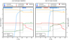 |
Fig. 12 Abundance profiles of the primary at different evolutionary stages as predicted by the evolutionary models. The legend at the top of each plot explains the colors indicating the dominating mixing processes. The H, He, C, N, and O abundances of the model are shown as solid lines while the observed surface CNO abundances are shown as dotted lines of the same respective color. The vertical black dotted line indicates the mass of the primary after mass transfer. Left panel: primary has depleted hydrogen in the core and is at the terminal age MS. Right panel: primary fills its Roche lobe and starts transferring mass. |
6.4 AzV 476 and its future evolution in the context of the most massive star population in the SMC
The binary components of AzV 476 are among the most luminous O stars in the entire SMC. Nevertheless, our analysis reveals that the mass of the O4 IV-III((f))p primary star is only Morb, 1 ≈ 20 M⊙. We estimate its initial mass to be Mini, 1 ≈ 33 M⊙ which is significantly lower than the most massive O stars in the Galaxy and the LMC (e.g., Ramírez-Agudelo et al. 2017; Gruner et al. 2019). This system therefore further exacerbates the problem with the deficiency of very massive O stars in the SMC (Ramachandran et al. 2019; Schootemeijer et al. 2021).
In the future, the primary in AzV 476 will evolve bluewards on the HRD, but it will never be able to lose its entire H-rich envelope. As its luminosity is on the edge of the least luminous observed WR star of the SMC (Shenar et al. 2016, 2020), it is unclear as to whether or not it will be able to develop an optically thick wind and become a WR star. Our evolutionary model predicts that the primary will have a final mass of Mfinal, 1 = 16 M⊙ at core helium exhaustion. The primary will probably collapse and form a BH (Heger et al. 2003). To our knowledge, no BH has yet been identified in the SMC.
After the primary collapse and the formation of a compact object, the system will consist of a MS star with a compact object. The MESA model predicts that the secondary will have Teff= 28 kK and log (L∕L⊙) = 4.85, at the halfway point of its remaining MS lifetime. We calculated a spectroscopic model of the secondary in this evolutionary stage and find that the secondary would be classified as a B0 V star. Its critical rotation makes the system a likely progenitor of a high-mass X-ray binary (HMXB) with a Be donor star. After the stellar model evolves beyond the MS, it undergoes a mass-transfer phase, offering an additional opportunity to show up as a HMXB. After large fractions of the secondary’s envelope are strippedoff, it will remain as a helium star with some hydrogen left on the surface with a luminosity around log (L∕L⊙) ≈ 4.9. Using the recent estimates from Sander & Vink (2020) for massive hydrogen-free stars, the L/M-ratio will be significantly too low to yield a sufficiently strong stellar wind for it to become optically thick at this metallicity (even when accounting for additional hydrogen and larger radii). Thus, our secondary star will most likely never appear as a WR star. With a final mass of Mfinal, 2 = 7 M⊙ at core helium depletion, the secondary is expected to explode as a supernova leaving a NS. With a final orbital period of about ≈ 100 d, this system is not expected to merge within a Hubble time. The impact of a supernova kick is neglected in our binary models; nevertheless, in principle, it could change the final orbital period of the system drastically.
7 Summary and conclusions
In this work, we study the earliest known O-type eclipsing binary in the SMC, AzV 476. We derived the masses of its companions using a spectroscopic analysis and by modeling its light- and RV curves. We compare the results with binary evolutionary models.
We conducted a quantitative analysis of the multi-phase spectra in the optical and UV obtained by the ESO VLT and the HST and supplemented by the FUSE spectroscopy in the far-UV. To this end we used the non-LTE stellar atmosphere model code PoWR. The spectra of both components were disentangled, allowing us to determine their masses, stellar, and wind parameters. Independently, we used the PHOEBE code to derive the stellar and the orbital parameters from the light curve in the I-band as well as RV curves. We employed the MESA code to compute detailed binary evolutionary models that are able to reproduce the observed stellar parameters in significant detail (see Table 6 and Fig. 11).
Our conclusions can be summarized as follows:
- (1)
The eclipsing binary AzV 476 harbors one of the most luminous O stars in the SMC. It consists of an O4 IV-III((f))p type primary and an O9.5: Vn type secondary. Single stars with similar spectral types typically have masses of Mexp, 1 = 49 M⊙ and Mexp, 2 = 16 M⊙.
- (2)
By analyzing the light curve and the RV curve consistently, we derive orbital masses of Morb, 1 = 20 M⊙ and Morb, 2 = 18 M⊙ for the binary components. We find that the primary has less than half of the mass that is expected from its spectral type. The modest mass of one of the most luminous stars in the SMC highlights the conspicuous deficiency of very massive O-type stars in this metal-poor galaxy.
- (3)
The spectroscopic masses agree within the uncertainties with the more reliable orbital masses, and they confirm a mass ratio of close to unity. The observed spectra reveal that the surface N abundance of the primary is enhanced while C and O abundances are reduced. These two aspects suggest a prior mass-transfer phase.
- (4)
The spectroscopic analysis uncovers that the mass-loss rate of the primary with log (Ṁ∕(M⊙ yr−1)) = −6.1 is ten times stronger compared to recent empirical prescriptions for single O stars in the SMC. Likely, this is due to its high L∕M ratio. Our empirical mass-loss rate is a factor of two higher compared to the one used in the evolutionary models. While for our primary the result as such is in line with standard theoretical predictions, this underlines that the present treatment of wind mass loss in stellar evolution models needs to be improved to properly account for the products of binary evolution.
- (5)
The current moderate mass of the primary can only be explained by binary evolutionary models. According to our favorite binary model, the initial mass of the primary was Mini, 1 = 33 M⊙, while the secondary formed with Mini, 2 = 18 M⊙. The system is ~6 Myr old.
- (6)
The binary evolutionary model confirms that this binary has undergone case B mass transfer and is now in a detached phase. The binary evolutionary model reveals that the primary must be core helium burning and that the observed CNO abundances correspond to those of the hydrogen shell burning layers.
- (7)
According to our binary evolution model, the primary will become a helium star (or maybe a WR star) with a portion of the hydrogen remaining in the envelope (XH < 50%) and finally collapse to a BH or NS. If the binary system stays bound after core-collapse, it might show up as a HMXB with a rapidly rotating Be-type donor. After core hydrogen depletion, the secondary is expected to expand and transfer mass onto the compact object, stripping off most of its hydrogen-rich envelope. The secondary will spend most of its late evolutionary phases in the blue part of the HRD as a helium star with a small fraction of hydrogen left in the envelope. However, due to its low L∕M ratio, it will never be able to display a WR-like spectrum. Finally, the secondary will collapse, and there is a small chance it will form a binary of compact objects that could potentially merge within a Hubble time.
The three different methods that we used to derive the stellar masses of the binary components show that the different mass estimates agree within their respective uncertainties (e.g., Table 6 and Fig. 11). Nonetheless, the different methods yield somewhat different results. We point out several difficulties that come along with the different methods applied, for instance when measuring surface gravity (see Fig. 5). Finally, we conclude that the earliest type eclipsing binary in the SMC, AzV 476, provides a unique laboratory for studying massive binaries at low metallicity.
Acknowledgements
We dedicate this publication to the late Dr. Rodolfo H. Barba, whose passing is a tragic loss to the astrophysicscommunity. As the original referee of this paper, he provided an outstandingly detailed and substantial report, which was extremely helpful and led to significant improvements of this work. Dr. Barba also provided us with the extracted TESS light curve of AzV 476 which resulted in the update in the orbital period. The authors thank Dr. Alex Fullerton for useful discussion and advise related to the FUSE spectroscopy and Soetkin Janssens for very helpful advises regarding the PHOEBE code. We gratefully thank the staff of the FUSE, HST, ESO telescopes for making the useful spectroscopic data publicly available. The results presented in this paper are based on observationsobtained with the NASA/ESA Hubble Space Telescope, retrieved from the Mikulski Archive for Space Telescopes (MAST) at the Space Telescope Science Institute (STScI). STScI is operated by the Association of Universities for Research in Astronomy, Inc. under NASA contract NAS 5-26555. Furthermore, its conclusions are based on observations collected at the European Southern Observatory (ESO) under the program 098.A-0049. The authors thank Andrea Mehner for preparing the OBs of the XSHOOTU project and the people on the management committee of XSHOOTU. This work has made use of data from the European Space Agency (ESA) mission Gaia (https://www.cosmos.esa.int/gaia), processed by the Gaia Data Processing and Analysis Consortium (DPAC, https://www.cosmos.esa.int/web/gaia/dpac/consortium). Funding for the DPAC has been provided by national institutions, in particular the institutions participating in the Gaia Multilateral Agreement. DP acknowledges financial support by the Deutsches Zentrum für Luft und Raumfahrt (DLR) grant FKZ 50 OR 2005. AACS is Öpik Research Fellow at Armagh Observatory & Planetarium. AACS and VR acknowledge support by the Deutsche Forschungsgemeinschaft (DFG – German Research Foundation) in the form of an Emmy Noether Research Group (grant number SA4064/1-1, PI Sander). JMA acknowledges support from the Spanish Government Ministerio de Ciencia through grant PGC2018-095 049-B-C22.
Appendix A RV determination
To determine the RV shift of a star during a specific phase we use a MCMC approach. In our code we use the synthetic spectra obtained from the spectral analysis and shift them until the shifted synthetic spectrum best matches the observed spectrum. In our procedure, we use the method described in the emcee documentation5 with small adjustments such that it fulfills our needs.
The probability function, a measure of how well the synthetic spectrum fits the observed one, consists of the combinationof a prior function (i.e., a function that limits the parameter space to reasonable numbers) and a likelihood function. Uniform distributions are used as prior functions to avoid biases towards specific RV shifts,
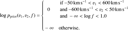 (A.1)
(A.1)
For the likelihood function we use the least square function and assume that the variance is underestimated by some fractional amount f,
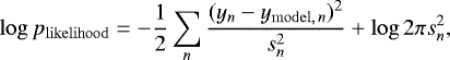 (A.2)
(A.2)
where
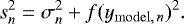 (A.3)
(A.3)
Using the above-mentioned functions, the probability function can be expressed as
 (A.4)
(A.4)
As recommended in the emcee documentation the starting values are initialized as tiny Gaussian balls around v1 = 300 km s−1, v2 = −300 km s−1 and log f = 0.0. To ensure a good converged posterior distribution, 32 walkers (i.e., individual Makrov chains) are used and each one is iterated for 5000 steps. We cut off the first 1000 steps to ensure that the chains are “burned-in” such that the remaining distribution resembles the posterior distribution. The uncertainties are based on the 16th, 50th, and 84th percentiles of the samples, corresponding to approximately 1σ deviation. To make these values readable for the PHOEBE code, which requires symmetric error margins, only the larger uncertainty is used.
For each of the components, we take the mean value of the RVs obtained from several absorption lines. The primary is causing most of the He II lines seen in the composite spectrum. Only the He II λ4025 line shows contributions from both components. The secondary contributes the majority of the observed He I absorption lines, but in many of them also the primary can be seen. We use the He II λ4025 line to fit both components and to obtain their RVs simultaneously, such that this line can be used as a cross-check to see if these fits are in agreement with the other lines that are purely from the primary, like He II λ4200, or the lines that are associated with the secondary. This gives us confidence that the RVs of the secondary obtained with this method are trustworthy. The obtained RVs of the primary and secondary can be found in Table A.1 and A.2.
This fitting procedure turns out to work well even for line complexes with contributions from both stars. Figure A.1 shows one of our fits of the He Iλ3819 region. The He Iλ3819 absorption line is present in both spectra. The absorption line of the primary is shifted redwards and the rotationally broadened absorption line of the secondary is shifted bluewards. This complex is blended by the blueshifted He II λ3813 absorption line of the primary.
This method requires sufficiently high S∕N observations. The MCMC code struggles with some of the He I lines that are associated with the secondary. In most cases, the problems emerge when the depth of the absorption lines is of the same order as the noise (i.e., the UVES spectra have a S∕N ~ 25). Moreover, some of the UVES spectra show a wavy pattern from the echelle orders. In some cases, these waves overlap with absorption lines, making an accurate RV determination almost impossible. All fits are inspected by eye and the observations that show the aforementioned issues are discarded from our analysis.
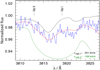 |
Fig. A.1 Radial-velocity fit of the synthetic spectrum to the observed He IIλ3813 and He I λ3819 absorption lines of the UVES spectrum with ID 10 (Table 1). The observed spectrum is shown as a solid blue line, our best fitting model as a dotted red line, the unweighted synthetic spectrum of the primary as a dashed black line, and the unweighted spectrum of the secondary as a dotted green line. The observed spectrum is convolved with a Gaussian with a FWHM = 0.2 Å and is corrected for the velocity of the SMC and the barycentric motion. The line identification marks correspond to the wavelengths of the absorption lines in the rest frame. |
RVs of the primary determined from different spectral lines.
RVs of the secondary determined from different spectral lines.
Appendix B Additional figures
B.1 Additional optical N III and N V lines
Figure B.1 shows N III and N V lines in our spectrum with the highest S∕N, the X-SHOOTER spectrum (ID 5 in Table 1, S∕N ~ 100). These lines are very weak and therefore barely visible in the spectrum. N V λ4604 is marginally in absorption, while N IIIλλ4634, 4641 appears in slight emission. Although nearly hidden in the noise, these weak features are reproduced by our final model (red-dotted).
B.2 Optical O IV and N IV lines
Walborn et al. (2004) suggest to use the optical O IV multiplets around 3400 Å and the N IV absorption lines at wavelengths 3463 Å, 3478 Å, 3483 Å and 3485 Å to derive the N and O abundances in hot massive stars. Luckily, the X-SHOOTER spectrum extends to such short wavelengths. Figure B.2 shows that the N IV lines of our final model are in agreement with the observation. However, for the O IV multiplet at wavelengths 3403 Å and 3414 Å the synthetic spectrum is in emission and not in absorption as observed. For the O IV λ3414 Å line, there is an ISM contribution from Co I that explains the observed absorption. Regarding the O IV 3403 Å line, we are not aware of any blending lines. However, this particular line is formed close to the onset of the wind and is sensitive to different details within the wind (e.g., temperature stratification, wind velocity law). As the other O IV multiplet λλ3381 Å−3389 Å can be well reproduced, we trust our determined O abundance, which is supported by other absorption lines in the UV.
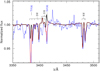 |
Fig. B.2 Observed (X-SHOOTER spectrum; ID 5 in Table 1) and synthetic spectra of the region around 3400 Å showing theO IV and N IV lines. The observed spectrum (blue) shows clear indications of ISM absorption lines. The black line isthe synthetic spectrum without a contribution of ISM lines. The spectrum with the modeled ISM lines is shown as red dotted line. The interstellar absorption arise in the Galactic foreground and in the SMC. |
B.3 Additional wind lines
As main diagnostic wind lines, the C IV resonance doublet in the UV and the Hα line in the optical are used. However, the He II λ1640 in the UV and the He II λ4868 in the optical are also sensitive to the stellar wind and are taken into account when adjusting the stellar parameters of our synthetic model. These lines are shown in Fig. B.3.
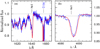 |
Fig. B.3 Observed (blue) and synthetic (red) He II lines that are sensitive to the wind parameters. The sharp interstellar absorptions arise in the Galactic foreground and in the SMC, and are also modeled with their respective RV shifts. (a) He II λ1640 line in the COS spectrum (ID 2 in Table 1). (b) He II λ4868 line in the X-SHOOTER spectrum (ID 5 in Table 1). |
B.4 Synthetic spectrum calculated with the stellar parameters from the MESA model
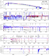 |
Fig. B.4 Spectral model calculated with the stellar parameters of the most favored binary evolutionary model. The plots and line styles are the same as in Figs. 9 and 10. In this plot we use a distance of d = 49 kpc to compensate the used lower luminosities of the binary components. This plot demonstrates that the predicted surface abundances of the binary evolutionary models are unable to reproduce the observed spectrum. The nitrogen abundance in this model is too strong as it overestimates all optical N IV lines and also predicts unseen N V absorption. The reduced hydrogen abundance leads to an increased helium abundance. This enrichment would produce too deep He II lines in the spectrum of the primary. |
References
- Abdul-Masih, M., Sana, H., Hawcroft, C., et al. 2021, A&A, 651, A96 [NASA ADS] [CrossRef] [EDP Sciences] [Google Scholar]
- Asplund, M., Grevesse, N., & Sauval, A. J. 2005, in Cosmic Abundances as Records of Stellar Evolution and Nucleosynthesis, eds. T. G. Barnes III, & F. N. Bash, (San Francisco: Astronomical Society of the Pacific), ASP Conf. Ser., 336, 25 [NASA ADS] [Google Scholar]
- Böhm-Vitense, E. 1958, Z. Astrophys., 46, 108 [Google Scholar]
- Bonanos, A. Z., Lennon, D. J., Köhlinger, F., et al. 2010, AJ, 140, 416 [NASA ADS] [CrossRef] [Google Scholar]
- Bouchet, P., Lequeux, J., Maurice, E., Prevot, L., & Prevot-Burnichon, M. L. 1985, A&A, 149, 330 [NASA ADS] [Google Scholar]
- Bouret, J.-C., Lanz, T., Hillier, D. J., et al. 2003, ApJ, 595, 1182 [NASA ADS] [CrossRef] [Google Scholar]
- Branton, D., Riley, A., et al. 2021, STIS Instrument Handbook, Version 20.0, Baltimore: STScI [Google Scholar]
- Brott, I., de Mink, S. E., Cantiello, M., et al. 2011, A&A, 530, A115 [NASA ADS] [CrossRef] [EDP Sciences] [Google Scholar]
- Cassinelli, J. P., & Olson, G. L. 1979, ApJ, 229, 304 [NASA ADS] [CrossRef] [Google Scholar]
- Castor, J. I., Abbott, D. C., & Klein, R. I. 1975, ApJ, 195, 157 [Google Scholar]
- Cignoni, M., Sabbi, E., Nota, A., et al. 2009, AJ, 137, 3668 [NASA ADS] [CrossRef] [Google Scholar]
- Conroy, K. E., Kochoska, A., Hey, D., et al. 2020, ApJS, 250, 34 [Google Scholar]
- Cutri, R. M., Skrutskie, M. F., van Dyk, S., et al. 2003, VizieR Online Data Catalog: II/246 [Google Scholar]
- De Propris, R., Rich, R. M., Mallery, R. C., & Howard, C. D. 2010, ApJ, 714, L249 [NASA ADS] [CrossRef] [Google Scholar]
- Dekker, H., D’Odorico, S., Kaufer, A., Delabre, B., & Kotzlowski, H. 2000, SPIE Conf. Ser., 4008, 534 [Google Scholar]
- Diaz-Cordoves, J., & Gimenez, A. 1992, A&A, 259, 227 [Google Scholar]
- Dionne, D., & Robert, C. 2006, ApJ, 641, 252 [NASA ADS] [CrossRef] [Google Scholar]
- Foreman-Mackey, D., Hogg, D. W., Lang, D., & Goodman, J. 2013, PASP, 125, 306 [Google Scholar]
- Gaia Collaboration (Prusti, T., et al.) 2016, A&A, 595, A1 [NASA ADS] [CrossRef] [EDP Sciences] [Google Scholar]
- Gaia Collaboration (Brown, A. G. A., et al.) 2021, A&A, 649, A1 [NASA ADS] [CrossRef] [EDP Sciences] [Google Scholar]
- Gilkis, A., Shenar, T., Ramachandran, V., et al. 2021, MNRAS, 503, 1884 [NASA ADS] [CrossRef] [Google Scholar]
- Gomel, R., Faigler, S., & Mazeh, T. 2021, MNRAS, 501, 2822 [CrossRef] [Google Scholar]
- Götberg, Y., Korol, V., Lamberts, A., et al. 2020, ApJ, 904, 56 [CrossRef] [Google Scholar]
- Gräfener, G., Koesterke, L., & Hamann, W.-R. 2002, A&A, 387, 244 [NASA ADS] [CrossRef] [EDP Sciences] [Google Scholar]
- Gruner, D., Hainich, R., Sander, A. A. C., et al. 2019, A&A, 621, A63 [NASA ADS] [CrossRef] [EDP Sciences] [Google Scholar]
- Hainich, R., Rühling, U., Todt, H., et al. 2014, A&A, 565, A27 [NASA ADS] [CrossRef] [EDP Sciences] [Google Scholar]
- Hainich, R., Pasemann, D., Todt, H., et al. 2015, A&A, 581, A21 [NASA ADS] [CrossRef] [EDP Sciences] [Google Scholar]
- Hainich, R., Shenar, T., Sander, A., Hamann, W. R., & Todt, H. 2017, in The Lives and Death-Throes of Massive Stars, ed. J. J. Eldridge, J. C. Bray, L. A. S. McClelland, & L. Xiao, 329, 171 [NASA ADS] [Google Scholar]
- Hamann, W.-R., & Gräfener, G. 2003, A&A, 410, 993 [CrossRef] [EDP Sciences] [Google Scholar]
- Hamann, W.-R., & Gräfener, G. 2004, A&A, 427, 697 [NASA ADS] [CrossRef] [EDP Sciences] [Google Scholar]
- Hamann, W.-R., & Koesterke, L. 1998a, A&A, 335, 1003 [NASA ADS] [Google Scholar]
- Hamann, W.-R., & Koesterke, L. 1998b, A&A, 333, 251 [NASA ADS] [Google Scholar]
- Hamann, W.-R., Gräfener, G., Oskinova, L., & Liermann, A. 2008, in Mass Loss from Stars and the Evolution of Stellar Clusters, eds. A. de Koter, L. J. Smith, & L. B. F. M. Waters, ASP Conf. Ser., 388, 171 [NASA ADS] [Google Scholar]
- Hammer, F., Yang, Y. B., Flores, H., Puech, M., & Fouquet, S. 2015, ApJ, 813, 110 [NASA ADS] [CrossRef] [Google Scholar]
- Heger, A., Langer, N., & Woosley, S. E. 2000, ApJ, 528, 368 [NASA ADS] [CrossRef] [Google Scholar]
- Heger, A., Fryer, C. L., Woosley, S. E., Langer, N., & Hartmann, D. H. 2003, ApJ, 591, 288 [CrossRef] [Google Scholar]
- Herrero, A., Kudritzki, R. P., Vilchez, J. M., et al. 1992, A&A, 261, 209 [NASA ADS] [Google Scholar]
- Hillier, D. J., & Miller, D. L. 1999, ApJ, 519, 354 [Google Scholar]
- Hillier, D. J., Koenigsberger, G., Nazé, Y., et al. 2019, MNRAS, 486, 725 [Google Scholar]
- Hirschauer, A. S., et al. 2021, Cosmic Origins Spectrograph Instrument Handbook, Version 13.0, Baltimore: STScI [Google Scholar]
- Holgado, G., Simón-Díaz, S., Haemmerlé, L., et al. 2020, A&A, 638, A157 [NASA ADS] [CrossRef] [EDP Sciences] [Google Scholar]
- Horvat, M., Conroy, K. E., Pablo, H., et al. 2018, ApJS, 237, 26 [Google Scholar]
- Hunter, I., Dufton, P. L., Smartt, S. J., et al. 2007, A&A, 466, 277 [NASA ADS] [CrossRef] [EDP Sciences] [Google Scholar]
- Jones, D., Conroy, K. E., Horvat, M., et al. 2020, ApJS, 247, 63 [Google Scholar]
- Kippenhahn, R., Ruschenplatt, G., & Thomas, H. C. 1980, A&A, 91, 175 [Google Scholar]
- Klencki, J., Nelemans, G., Istrate, A. G., & Pols, O. 2020, A&A, 638, A55 [NASA ADS] [CrossRef] [EDP Sciences] [Google Scholar]
- Koenigsberger, G., Morrell, N., Hillier, D. J., et al. 2014, AJ, 148, 62 [Google Scholar]
- Kolb, U., & Ritter, H. 1990, A&A, 236, 385 [NASA ADS] [Google Scholar]
- Langer, N. 1987, A&A, 171, L1 [NASA ADS] [Google Scholar]
- Langer, N., Fricke, K. J., & Sugimoto, D. 1983, A&A, 126, 207 [NASA ADS] [Google Scholar]
- Mahy, L., Almeida, L. A., Sana, H., et al. 2020, A&A, 634, A119 [NASA ADS] [CrossRef] [EDP Sciences] [Google Scholar]
- Maíz Apellániz, J. 2019, MGB: Interactive spectral classification code [Google Scholar]
- Maíz Apellániz, J., Pellerin, A., Barbá, R. H., et al. 2012, in Proceedings of a Scientific Meeting in Honor of Anthony F. J. Moffat, eds. L. Drissen, C. Robert, N. St-Louis, & A. F. J. Moffat, ASP Conf. Ser., 465, 484 [Google Scholar]
- Marchant, P. 2016, PhD thesis, Rheinischen Friedrich-Wilhelms-Universität Bonn [Google Scholar]
- Markova, N., & Puls, J. 2015, in New Windows on Massive Stars, eds. G. Meynet, C. Georgy, J. Groh, & P. Stee, Vol. 307, 117 [Google Scholar]
- Markova, N., Puls, J., & Langer, N. 2018, A&A, 613, A12 [NASA ADS] [CrossRef] [EDP Sciences] [Google Scholar]
- Martins, F., & Palacios, A. 2021, A&A, 645, A67 [EDP Sciences] [Google Scholar]
- Massa, D., Fullerton, A. W., & Prinja, R. K. 2017, MNRAS, 470, 3765 [CrossRef] [Google Scholar]
- Massey, P., Puls, J., Pauldrach, A. W. A., et al. 2005, ApJ, 627, 477 [NASA ADS] [CrossRef] [Google Scholar]
- Mazeh, T. 2008, in EAS Pub. Ser., 29, eds. M. J. Goupil, & J. P. Zahn, 1 [NASA ADS] [CrossRef] [EDP Sciences] [Google Scholar]
- Morrell, N., Ostrov, P., Massey, P., & Gamen, R. 2003, MNRAS, 341, 583 [NASA ADS] [CrossRef] [Google Scholar]
- Muraoka, K., Homma, A., Onishi, T., et al. 2017, ApJ, 844, 98 [NASA ADS] [CrossRef] [Google Scholar]
- Nidever, D. L., Monachesi, A., Bell, E. F., et al. 2013, ApJ, 779, 145 [Google Scholar]
- Nieuwenhuijzen, H., & de Jager, C. 1990, A&A, 231, 134 [NASA ADS] [Google Scholar]
- Oegerle, W., Murphy, E., & Kriss, J. 2000, The FUSE Data Handbook, Version 1.1 [Google Scholar]
- Oskinova, L. M., Todt, H., Ignace, R., et al. 2011, MNRAS, 416, 1456 [NASA ADS] [CrossRef] [Google Scholar]
- Pawlak, M., Soszyński, I., Udalski, A., et al. 2016, Acta Astron., 66, 421 [Google Scholar]
- Paxton, B., Cantiello, M., Arras, P., et al. 2013, ApJS, 208, 4 [Google Scholar]
- Penny, L. R., & Gies, D. R. 2009, ApJ, 700, 844 [Google Scholar]
- Prša, A. 2011, PHOEBE Scientific Reference, Version 0.30 [Google Scholar]
- Prša, A., & Zwitter, T. 2005, ApJ, 628, 426 [Google Scholar]
- Prša, A., Conroy, K. E., Horvat, M., et al. 2016, ApJS, 227, 29 [Google Scholar]
- Ramachandran, V., Hamann, W. R., Hainich, R., et al. 2018, A&A, 615, A40 [NASA ADS] [CrossRef] [EDP Sciences] [Google Scholar]
- Ramachandran, V., Hamann, W. R., Oskinova, L. M., et al. 2019, A&A, 625, A104 [NASA ADS] [CrossRef] [EDP Sciences] [Google Scholar]
- Ramírez-Agudelo, O. H., Sana, H., de Koter, A., et al. 2017, A&A, 600, A81 [NASA ADS] [CrossRef] [EDP Sciences] [Google Scholar]
- Reindl, N., Rauch, T., Parthasarathy, M., et al. 2014, A&A, 565, A40 [NASA ADS] [CrossRef] [EDP Sciences] [Google Scholar]
- Rivero González, J. G., Puls, J., Massey, P., & Najarro, F. 2012, A&A, 543, A95 [NASA ADS] [CrossRef] [EDP Sciences] [Google Scholar]
- Sander, A. A. C., & Vink, J. S. 2020, MNRAS, 499, 873 [Google Scholar]
- Sander, A., Shenar, T., Hainich, R., et al. 2015, A&A, 577, A13 [NASA ADS] [CrossRef] [EDP Sciences] [Google Scholar]
- Sanyal, D., Grassitelli, L., Langer, N., & Bestenlehner, J. M. 2015, A&A, 580, A20 [NASA ADS] [CrossRef] [EDP Sciences] [Google Scholar]
- Schneider, F. R. N., Langer, N., de Koter, A., et al. 2014, A&A, 570, A66 [NASA ADS] [CrossRef] [EDP Sciences] [Google Scholar]
- Schootemeijer,A., Langer, N., Lennon, D., et al. 2021, A&A, 646, A106 [NASA ADS] [CrossRef] [EDP Sciences] [Google Scholar]
- Seaton, M. J. 1979, MNRAS, 187, 73P [NASA ADS] [CrossRef] [Google Scholar]
- Shara, M. M., Crawford, S. M., Vanbeveren, D., et al. 2020, MNRAS, 492, 4430 [NASA ADS] [CrossRef] [Google Scholar]
- Shenar, T., Oskinova, L., Hamann, W. R., et al. 2015, ApJ, 809, 135 [Google Scholar]
- Shenar, T., Hainich, R., Todt, H., et al. 2016, A&A, 591, A22 [NASA ADS] [CrossRef] [EDP Sciences] [Google Scholar]
- Shenar, T., Sablowski, D. P., Hainich, R., et al. 2019, A&A, 627, A151 [NASA ADS] [CrossRef] [EDP Sciences] [Google Scholar]
- Shenar, T., Gilkis, A., Vink, J. S., Sana, H., & Sander, A. A. C. 2020, A&A, 634, A79 [NASA ADS] [CrossRef] [EDP Sciences] [Google Scholar]
- Simón-Díaz, S., & Herrero, A. 2014, A&A, 562, A135 [NASA ADS] [CrossRef] [EDP Sciences] [Google Scholar]
- Soker, N. 2000, A&A, 357, 557 [NASA ADS] [Google Scholar]
- Sota, A., Maíz Apellániz, J., Walborn, N. R., et al. 2011, ApJS, 193, 24 [Google Scholar]
- Sota, A., Maíz Apellániz, J., Morrell, N. I., et al. 2014, ApJS, 211, 10 [Google Scholar]
- Spruit, H. C. 2002, A&A, 381, 923 [CrossRef] [EDP Sciences] [Google Scholar]
- Tatton, B. L., van Loon, J. T., Cioni, M. R. L., et al. 2021, MNRAS, 504, 2983 [NASA ADS] [CrossRef] [Google Scholar]
- Todt, H., Sander, A., Hainich, R., et al. 2015, A&A, 579, A75 [NASA ADS] [CrossRef] [EDP Sciences] [Google Scholar]
- Trundle, C., Dufton, P. L., Hunter, I., et al. 2007, A&A, 471, 625 [NASA ADS] [CrossRef] [EDP Sciences] [Google Scholar]
- Vanbeveren, D., Mennekens, N., Shara, M. M., & Moffat, A. F. J. 2018, A&A, 615, A65 [NASA ADS] [CrossRef] [EDP Sciences] [Google Scholar]
- Vernet, J., Dekker, H., D’Odorico, S., et al. 2011, A&A, 536, A105 [NASA ADS] [CrossRef] [EDP Sciences] [Google Scholar]
- Vink, J. S., & Sander, A. A. C. 2021, MNRAS, 504, 2051 [NASA ADS] [CrossRef] [Google Scholar]
- Vink, J. S., de Koter, A., & Lamers, H. J. G. L. M. 2001, A&A, 369, 574 [NASA ADS] [CrossRef] [EDP Sciences] [Google Scholar]
- Vos, J., Østensen, R. H., Marchant, P., & Van Winckel, H. 2015, A&A, 579, A49 [NASA ADS] [CrossRef] [EDP Sciences] [Google Scholar]
- Walborn, N. R., Lennon, D. J., Heap, S. R., et al. 2000, PASP, 112, 1243 [Google Scholar]
- Walborn, N. R., Howarth, I. D., Lennon, D. J., et al. 2002, AJ, 123, 2754 [NASA ADS] [CrossRef] [Google Scholar]
- Walborn, N. R., Morrell, N. I., Howarth, I. D., et al. 2004, ApJ, 608, 1028 [NASA ADS] [CrossRef] [Google Scholar]
- Walborn, N. R., Sana, H., Simón-Díaz, S., et al. 2014, A&A, 564, A40 [NASA ADS] [CrossRef] [EDP Sciences] [Google Scholar]
- Weidner, C., & Vink, J. S. 2010, A&A, 524, A98 [NASA ADS] [CrossRef] [EDP Sciences] [Google Scholar]
- Wilson, R. E. 1990, ApJ, 356, 613 [Google Scholar]
- Wright, J. T., & Eastman, J. D. 2014, PASP, 126, 838 [Google Scholar]
- Zacharias, N., Finch, C. T., Girard, T. M., et al. 2013, AJ, 145, 44 [Google Scholar]
The shorter wavelengths in the FUSE range are largely contaminated by interstellar features that yield no information about the stellar parameters.
All Tables
List of all spectra of AzV 476 used in this work and their associated orbital phase.
Summary of the stellar parameters of both stellar components obtained from the different methods.
All Figures
|
Fig. 1 Phased OGLE I-band and TESS light curves around the primary eclipse. Left panel: light curve phased according to the ephemeris from the OGLE catalog. Right panel: light curve phased according to the ephemeris we derive in this work by fitting the primary’s eclipses of the TESS light curve. |
| In the text | |
|
Fig. 2 Upper panel: phased OGLE I-band light curve of AzV 476 (blue dots) and the best fit obtained with the PHOEBE code (red line). Above the light curve, the spectral IDs of all used spectra (see Table 1) are indicated. Lower panel: observed (triangles) and fitted (solid lines) RV curves for the primary (green) and secondary (red). The fits of the light-curve fit and the RVs are consistently obtained by the PHOEBE code. |
| In the text | |
|
Fig. 3 X-shooter spectrum (ID 5 in Table 1) displayed in blue and one of the UVES spectra (ID 10 in Table 1) in red. The spectra are convolved with a Gaussian with an FWHM = 0.4 Å to reduce the noise and to make the RV shifts visible. The region containing Hγ, He I λ4387, and He I λ4471 lines is shown. In the spectrum shown by the red line, the primary’s spectrum is redshifted (see Hγ), while the secondary’s spectrum (broadened He I lines) is blueshifted. We note that the primary also partially contributes to the He I lines. |
| In the text | |
|
Fig. 4 Same as Fig. 3, but now for the region around the He I λ3819 and Hϵ lines. Most of the lines, including He I λ3926, are redshifted and associated with the primary, while the He I λ3819 line which isassociated with the secondary is blueshifted. |
| In the text | |
|
Fig. 5 Selected regions of the X-shooter spectrum (ID 5 in Table 1) compared to different synthetic spectra. The observed spectrum, corrected for the velocity of the SMC and the barycentric motion, is shown as a solid blue line. The red dotted line is our best-fitting model which consists of the primary with Teff, 1 = 42 kK and log g*, 1 = 3.7 and the secondary with Teff, 2 = 32 kK and log g*, 1 = 4.0. The gray solid line is again a combined synthetic spectrum of the primary and secondary, but this time the surface gravity of the primary has been reduced to log g*, 1= 3.6 (and the temperature and mass-loss rate are slightly adjusted so that the spectrum matches the observations) while the parameters of the secondary are kept fixed. The line identification marks correspond to the wavelengths in the rest frame. Panel a shows the Hγ line, in which the red wing is dominated by the primary and the blue wing by the secondary. Panel b shows the He II λ5412 absorption line, which is dominated by the primary and is sensitive to surface gravity. Panel c shows the region of He II λ6528 and Hα. While the Hα wings are only barely affected by the change in logg*, 1, the He II λ6528 line is more sensitive to it. |
| In the text | |
|
Fig. 6 Part of the observed FUSE spectrum (ID 1 in Table 1) covering the wavelength range of the LiF2 channel – the same as used by Penny & Gies (2009) to determine the projected rotational velocity. The observed spectrum, corrected for the velocity of the SMC, is shown as a solid blue line. The red dotted line is our best-fitting model with the primary’s projected rotational velocity v1 sin i = 140 km s−1. The gray solid line is another model where the primary’s projected rotational velocity is reduced to v1 sin i = 140 km s−1. The line identification marks correspond to the wavelengths in the rest frame. |
| In the text | |
|
Fig. 7 Observed (blue) and synthetic (red) C IV resonance doublet of our final model. The individual primary and secondary spectra are shown as dotted black and green lines, respectively. The sharp interstellar absorptions arise in the Galactic foreground and in the SMC, and are also modeled with their respective RV shifts. (a) COS observation (ID 2 in Table 1) (b) STIS observation (ID 3 in Table 1). |
| In the text | |
|
Fig. 8 Observed X-shooter spectrum (ID 5 in Table 1) and synthetic spectra of selected regions that show nitrogen emission lines. The observed spectrum is shown as a solid blue line, while the dotted red line is our best-fitting model. The observed spectrum is corrected for the velocity of the SMC and the barycentric motion. The line identification marks correspond to the wavelengths in the rest frame. Panel a shows the area around the N IV λ4057. Panel b shows the region of N III λλ4511−4523, N V λλ4604, 4620, and N III λλ4634, 4641. The N III and N V lines are not observable in the spectrum. Panel c shows the region of the N IV λλ7103−7129 complex. |
| In the text | |
|
Fig. 9 Spectral fit for AzV 476. Top panel: SED. Flux-calibrated observations (blue lines) are the FUSE (1), COS (2), STIS (4), and X-shooter (5) spectra as listed in Table 1. The light blue squares are the photometric UBVRIJHK data as listed in Table 2. The model SED composed of both stellar components is shown as a dashed red line, while the individual SEDs of the primary and the secondary are shown as dotted black and green lines, respectively.Lower panels: normalized FUSE (1), COS (2), and STIS (4) spectra. The number in the upper left corner corresponds to the ID given to a specific spectrum as listed in Table 1. The line styles are the same as in the top panel. The synthetic spectra are calculated with the model parameters compiled in Table 6 (“Spectroscopy” columns). |
| In the text | |
|
Fig. 10 Same as Fig. 9, but now the normalized optical X-shooter spectra (ID 5 in Table 1) are shown. |
| In the text | |
|
Fig. 11 HRD showing the positions of each binary component according to the spectroscopic and orbital analysis, and the best fitting binary evolutionary tracks. The results of the spectroscopic analysis are shown as triangles and the orbital analysis as upside-down triangles. The positions of the primary and secondary are marked in green and red, respectively. The shaded areas indicate the respective error-ellipses. Evolutionary tracks (solid lines) of both binary componentsare according to the best fitting binary model calculated with MESA (see Sect. 5.2). The tracks are labeled by their initial masses. The black dots on the tracks correspond to equidistant time-steps of 0.1 Myr to emphasize the most probable observable phases. The light blue dots mark the best-fitting model. |
| In the text | |
|
Fig. 12 Abundance profiles of the primary at different evolutionary stages as predicted by the evolutionary models. The legend at the top of each plot explains the colors indicating the dominating mixing processes. The H, He, C, N, and O abundances of the model are shown as solid lines while the observed surface CNO abundances are shown as dotted lines of the same respective color. The vertical black dotted line indicates the mass of the primary after mass transfer. Left panel: primary has depleted hydrogen in the core and is at the terminal age MS. Right panel: primary fills its Roche lobe and starts transferring mass. |
| In the text | |
|
Fig. A.1 Radial-velocity fit of the synthetic spectrum to the observed He IIλ3813 and He I λ3819 absorption lines of the UVES spectrum with ID 10 (Table 1). The observed spectrum is shown as a solid blue line, our best fitting model as a dotted red line, the unweighted synthetic spectrum of the primary as a dashed black line, and the unweighted spectrum of the secondary as a dotted green line. The observed spectrum is convolved with a Gaussian with a FWHM = 0.2 Å and is corrected for the velocity of the SMC and the barycentric motion. The line identification marks correspond to the wavelengths of the absorption lines in the rest frame. |
| In the text | |
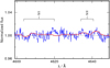 |
Fig. B.1 Same as Fig. 8, but now zoomed on optical N III and N V lines. |
| In the text | |
|
Fig. B.2 Observed (X-SHOOTER spectrum; ID 5 in Table 1) and synthetic spectra of the region around 3400 Å showing theO IV and N IV lines. The observed spectrum (blue) shows clear indications of ISM absorption lines. The black line isthe synthetic spectrum without a contribution of ISM lines. The spectrum with the modeled ISM lines is shown as red dotted line. The interstellar absorption arise in the Galactic foreground and in the SMC. |
| In the text | |
|
Fig. B.3 Observed (blue) and synthetic (red) He II lines that are sensitive to the wind parameters. The sharp interstellar absorptions arise in the Galactic foreground and in the SMC, and are also modeled with their respective RV shifts. (a) He II λ1640 line in the COS spectrum (ID 2 in Table 1). (b) He II λ4868 line in the X-SHOOTER spectrum (ID 5 in Table 1). |
| In the text | |
|
Fig. B.4 Spectral model calculated with the stellar parameters of the most favored binary evolutionary model. The plots and line styles are the same as in Figs. 9 and 10. In this plot we use a distance of d = 49 kpc to compensate the used lower luminosities of the binary components. This plot demonstrates that the predicted surface abundances of the binary evolutionary models are unable to reproduce the observed spectrum. The nitrogen abundance in this model is too strong as it overestimates all optical N IV lines and also predicts unseen N V absorption. The reduced hydrogen abundance leads to an increased helium abundance. This enrichment would produce too deep He II lines in the spectrum of the primary. |
| In the text | |
Current usage metrics show cumulative count of Article Views (full-text article views including HTML views, PDF and ePub downloads, according to the available data) and Abstracts Views on Vision4Press platform.
Data correspond to usage on the plateform after 2015. The current usage metrics is available 48-96 hours after online publication and is updated daily on week days.
Initial download of the metrics may take a while.