| Issue |
A&A
Volume 659, March 2022
|
|
|---|---|---|
| Article Number | A50 | |
| Number of page(s) | 16 | |
| Section | The Sun and the Heliosphere | |
| DOI | https://doi.org/10.1051/0004-6361/202141414 | |
| Published online | 04 March 2022 | |
Measuring the F-corona intensity through time correlation of total and polarized visible light images
1
INAF – Osservatorio Astrofisico di Arcetri, Largo Enrico Fermi 5, 50125 Florence, Italy
e-mail: This email address is being protected from spambots. You need JavaScript enabled to view it.
2
Department of Physics and Astronomy, University of Padova, Via F. Marzolo 8, 35131 Padova, Italy
e-mail: This email address is being protected from spambots. You need JavaScript enabled to view it.
3
INAF – Osservatorio Astronomico di Padova, Vicolo dell’Osservatorio 5, 35122 Padova, Italy
4
INAF – Osservatorio Astrofisico di Catania, Via Santa Sofia 78, 95123 Catania, Italy
5
Department of Physics and Astronomy, University of Florence, Largo Enrico Fermi 2, 50125 Firenze, Italy
6
INAF – Osservatorio Astrofisico di Torino, Via Osservatorio, 20, 10025 Pino Torinese, Turin, Italy
7
Department of Physics and Astronomy, University of Catania, Via Santa Sofia 64, 95123 Catania, Italy
8
Max Planck Institute for Solar System Research, Justus-von-Liebig-Weg 3, 37077 Göttingen, Germany
Received:
28
May
2021
Accepted:
3
December
2021
Abstract
We present a new correlation method for deriving the F-corona intensity distribution, which is based on the analysis of the evolution of the total and polarized visible light (VL) images. We studied the one-month variation profiles of the total and polarized brightness acquired with Large Angle Spectrometric COronagraph and found that in some regions they are highly correlated. Assuming that the F-corona does not vary significantly on a timescale of one month, we estimated its intensity in the high-correlation regions and reconstructed the corresponding intensity maps both during the solar-minimum and solar-maximum periods. Systematic uncertainties were estimated by performing dedicated simulations. We compared the resulting F-corona images with those determined using the inversion technique and found that the correlation method provides a smoother intensity distribution. We also obtained that the F-corona images calculated for consecutive months show no significant variation. Finally, we note that this method can be applied to the future high-cadence VL observations carried out with the Metis/Solar Orbiter coronagraph.
Key words: Sun: corona / solar wind
© ESO 2022
1. Introduction
The brightness of the solar corona in visible light (VL) consists mainly of the contribution from the emission of (1) the K-corona, which arises from the Thomson scattering of photospheric light by free electrons, and (2) the F-corona, which originates from diffraction or scattering of the photospheric emission by the dust grains. Due to the different emission mechanisms, these two components possess quite different properties. The K-corona is observed with numerous asymmetric bright features (e.g., streamers). It is, on average, fainter than the F-corona, especially at high altitudes (≳3–4 R⊙, see e.g., Koutchmy & Lamy 1985). Radial profiles of the K-corona emission are steeper than those of the F-corona. It can be shown, for example, that the intensity profiles reported in Saito et al. (1977) for the solar minimum at heliocentric distances from 2 R⊙ to 5 R⊙ are well described by a power-law function f(r)∝r−n with the exponent n equal to 2.2 and 2.7 for the F-corona profiles along the equator and pole, respectively, and n equal to 4.3 and 4.5 for those of the K-corona. The emission from the K-corona is highly polarized (Minnaert 1930), whereas the F-corona is known to be almost unpolarized up to ∼20 R⊙ (see discussion in Lamy et al. 2021). According to the model of Blackwell & Petford 1966, the polarization of the F-corona rises from 0.05% at 5 R⊙ to 0.95% at 20 R⊙. Apart from the existence of so-called dust-free zone in the close vicinity of the Sun (see Howard et al. 2019 and references therein), the F-corona is known to be not coupled with the solar activity. Ragot & Kahler (2003), however, predicted the solar cycle variations of the F-corona brightness due to the interaction between coronal mass ejections (CMEs) and the dust grains. The significance of this effect is yet to be measured. The F-corona is also believed to be more stable than the K-corona (Morgan & Habbal 2007; Llebaria et al. 2021). Observations reveal a nearly symmetric brightness distribution of the F-corona with smooth intensity contours of super-elliptical shape, which becomes more eccentric at high elongations (Koutchmy & Lamy 1985; Stauffer et al. 2018; Llebaria et al. 2021).
Both the separation of the emission from the K- and F- coronae and the accurate determination of the corresponding intensity maps are necessary to perform detailed studies of the electron density distribution within the solar corona and the interplanetary dust. One method for separating the K and F components is based on the inversion technique (van de Hulst 1950), which assumes a certain level of symmetry in the electron density distribution. By inverting the polarized VL images, it is possible to calculate the electron density profiles and subsequently derive the image of the K-corona. The intensity map of the F-corona can be then determined as a difference between the total brightness and K-corona images (see e.g. Saito et al. 1977; Dolei et al. 2015). Hayes et al. (2001) proposed accounting for the contamination from the F-corona by subtracting a minimum brightness of each pixel from the total brightness images acquired over a time interval of 56 days, centered on the day of the observation. Adjusting the empirical model of the F-corona, Hayes et al. (2001) managed to minimize the contribution of the residual features of the K-corona to the F-corona map. Since this method is image-dependent, it is of limited application for the analysis of large data sets. More sophisticated techniques to determine an empirical background model of the VL images were later developed by, for example, Morrill et al. (2006), Morgan & Habbal (2010), Stenborg & Howard (2017), and references therein. These techniques are appropriate for studying the dynamic structures of the K-corona such as CMEs. Another approach for separating the K- and F- coronae is used in Lamy et al. (1997), Quémerais & Lamy (2002), Lamy et al. (2020). In these works the intensity maps of the K-corona were determined directly from the polarized brightness images using the model of the K-corona polarization pK(r). Llebaria et al. (2021), in turn, performed a careful restoration of the K and F components of the solar corona using the results of Lamy et al. (2020), who carried out a detailed characterization of the polarimetric channel of the Large Angle Spectrometric COronagraph (LASCO-C2, Brueckner et al. 1995) – an instrument on board the Solar and Heliospheric Observatory (SOHO, Domingo et al. 1995). Recently, Boe et al. (2021) presented a novel technique for separating emission from the K- and F-coronae at low altitudes (up to a few solar radii) based on the color analysis of the total solar eclipse data.
In this work, we present a new correlation method for deriving the F-corona intensity maps, which was developed using the total and polarized VL images of the LASCO instrument. We studied the evolution of the total and polarized brightness extracted from the LASCO-C2 images during a one-month time interval, and found that in some regions they are highly correlated. Assuming that the typical timescale of the F-corona variations is longer than one month, we estimated its brightness in these high-correlation regions. Our method does not require any specific assumption on the geometry of the electron density distribution and/or on the profile of the K-corona polarization. Resulting F-corona intensity maps have been compared with those obtained by means of the inversion technique.
The paper is organized as follows. Details on the selected data set and the data reduction are reported in Sect. 2. The correlation and inversion methods are described in Sect. 3. The main results are summarized in Sect. 4. The discussion and conclusions follow in Sects. 5 and 6, respectively.
2. Observations and data reduction
In these studies, we used LASCO-C2 images acquired with the Orange filter (540–640 nm). The analyzed data set covers four months that have a high number of polarized brightness observations (∼100 per month). These were May and June 2001 (solar maximum) and March and April 2008 (solar minimum).
The raw data (level “0.5”) were downloaded from the Virtual Solar Observatory (VSO)1. The reduced and calibrated (level “1”) total brightness images were obtained with the SolarSoftware package (Freeland & Handy 1998) routine reduce_level_1.pro. The calibrated polarized brightness images were downloaded from the corresponding LASCO data archive2. Each pixel of the calibrated maps provides the corona intensity in mean solar brightness (MSB) units. The images which contain large areas with zero intensity (missing blocks) were excluded from the analysis. The total number of VL images used in our analysis is reported in Table 1.
Number of total (B) and polarized (pB) brightness images used in this work.
In order to unify the format of total and polarized brightness images and apply the inversion technique (see Sect. 3.1), we converted all maps from Cartesian (x, y) to polar (r, ϕ) coordinates. For this, we determined the total and polarized brightness for a grid of polar coordinates, in which the radial r-axis ranges from 2.5 to 6.2 R⊙ with a step of 0.01 R⊙, and the polar angle ϕ-axis ranges from 0° to 360° with a step of 1°. The polar angle is measured counterclockwise from the west solar equator.
3. Measuring the F-corona intensity
The total brightness (B) images contain the emission from the K-corona (K), F-corona (F), and scattered/stray light (S):
 (1)
(1)
where pK and uK are the polarized and unpolarized fractions of the K-corona, respectively. The instrumental stray light is known to be unpolarized (see e.g., Llebaria et al. 2021) and the polarization of the F-corona does not exceed 0.06% below 6 R⊙ (adopted from Blackwell & Petford 1966). So that, even though the F-corona can be 10–100 times brighter than the K-corona at 6 R⊙ (see e.g., profiles in Koutchmy & Lamy 1985; Dolei et al. 2015), the polarized brightness (pB) maps can be considered as dominated by the emission from the K-corona, and, therefore, pK ≈ pB. The systematic errors introduced by neglecting the polarization of the F-corona are discussed in Sect. 5.5.
We point out that in our analysis we did not take into account the contribution from the stray light (S = 0). As a consequence, the resulting F-corona images are contaminated by the stray light of the LASCO-C2 instrument. Separating these two components is beyond the scope of this paper. The contamination from the stray light is evaluated and discussed in Sect. 5.6.
Taking into account that pK ≈ pB and (F + S)≡F, Eq. (1) can be then rewritten as follows:
 (2)
(2)
One of the possible ways to estimate F is to calculate the K-corona intensity from the pB map through the inversion technique (Sect. 3.1) and, then, to subtract it from the total brightness image. Another way is to obtain F directly from the data of the total and polarized brightness in the regions where B and pB are highly correlated (Sect. 3.2).
3.1. Inversion method
The intensity of the F-corona can be calculated using the quasi-simultaneous total and polarized brightness observations through the inversion technique (see e.g., Saito et al. 1977; Dolei et al. 2015). Assuming that the electron density ne is symmetric with respect to the plane of the sky (POS) along the line of sight (LOS), and that it is a function of the heliocentric distance r only, one can derive the following (van de Hulst 1950; Hayes et al. 2001):
![Mathematical equation: $$ \begin{aligned} K(x) = C_{\rm cf} \int _x^\infty n_{\rm e}(r) \left[\left(\frac{2r^2}{x^2} -1\right)A(r) + B(r)\right] \frac{x^2}{r\sqrt{r^2-x^2}} \mathrm{d} r \,, \end{aligned} $$](/articles/aa/full_html/2022/03/aa41414-21/aa41414-21-eq3.gif) (3)
(3)
![Mathematical equation: $$ \begin{aligned} pB(x) = C_{\rm cf} \int _x^\infty n_{\rm e}(r) [A(r) - B(r)] \frac{x^2}{r\sqrt{r^2-x^2}} \mathrm{d} r \, , \end{aligned} $$](/articles/aa/full_html/2022/03/aa41414-21/aa41414-21-eq4.gif) (4)
(4)
where x is the heliocentric distance projected on the POS and Ccf is a unit conversion factor. The adopted geometry is illustrated in Fig. 1. The geometric factors A and B can be derived from the following relations (van de Hulst 1950):
![Mathematical equation: $$ \begin{aligned} \begin{split} 2A + B&= \frac{1-q}{1-q/3} \left[ 2(1-\cos \gamma ) \right] \\&\quad + \frac{q}{1-q/3} \left[ 1 - \frac{\cos ^2\gamma }{\sin \gamma } \log \frac{1+\sin \gamma }{\cos \gamma } \right] \,, \end{split} \end{aligned} $$](/articles/aa/full_html/2022/03/aa41414-21/aa41414-21-eq5.gif) (5)
(5)
![Mathematical equation: $$ \begin{aligned} \begin{split} 2A - B&= \frac{1-q}{1-q/3} \left[ \frac{2}{3} (1-\cos ^3\gamma ) \right] \\&\quad + \frac{q}{1-q/3} \left[ \frac{1}{4} + \frac{\sin ^2\gamma }{4} - \frac{\cos ^4\gamma }{4\sin \gamma } \log \frac{1+\sin \gamma }{\cos \gamma } \right] \, . \end{split} \end{aligned} $$](/articles/aa/full_html/2022/03/aa41414-21/aa41414-21-eq6.gif) (6)
(6)
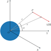 |
Fig. 1. Illustration of the geometry used in the inversion technique. The origin of the coordinate system (O) is placed at the center of the Sun. The pixel of interest P is in the plane of sky YOZ. The line of sight (LOS) parallel to the OX-axis is shown as the red arrow. The OZ-axis points to the north pole of the Sun |
In Eqs. (5) and (6), sin γ corresponds to R⊙/r, whereas q is the coefficient of the limb darkening taken equal to 0.63 (as e.g. in Antonucci et al. 2020).
We calculated the electron density distribution inverting the polarized brightness images as explained in Hayes et al. (2001) and Dolei et al. (2015). For this, we determined the radial profiles ne(r) of the electron density assuming that they follow the polynomial form:  . We substituted ne in Eq. (4) with the polynomial expression and performed the least-squares fitting of the resulting function pB(x) to the polarized brightness profile observed with LASCO-C2 at each polar angle ϕ. As a result, we obtained the coefficients αk and, therefore, the density profiles ne(r). For further details on this procedure, we refer the reader to Hayes et al. (2001). Then, we determined the K-corona intensity map Kinv by means of Eq. (3). The F-corona model (Finv) was calculated as the difference between the total brightness image that follows the pB acquisition of interest and the K-corona map. In the typical LASCO-C2 acquisition sequences the time separation between polarized and the immediately following total brightness images is on the order of ∼10 min. An example of resulting images of ne, K-corona, and F-corona, together with the LASCO-C2 B and pB intensity maps are shown in Fig. 2.
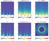 |
Fig. 2. Polarized (pB, top left panel) and total (B, top mid panel) brightness images obtained with LASCO-C2. pB image was acquired on June 1, 2001 at 9:00, whereas the B image was acquired on June 1, 2001 at 09:07. The electron density ne (bottom left panel), K-corona Kinv (bottom mid panel) and F-corona Finv maps (right panels) are calculated using the inversion technique (see Sect. 3.1). Finv is shown in polar and Cartesian coordinates. The horizontal axis corresponds to the polar angle ϕ in degrees, whereas the vertical axis is the heliocentric distance r in the R⊙ units in all panels except the bottom right, for which both axes correspond to the heliocentric distance. The color bar represents the intensity in MSB units in all panels except the ne map, for which it represents the density in cm−3 units. |
F-corona maps calculated with this technique usually have distinct faint features (e.g., at ϕ equal to ∼90° and ∼180° in Fig. 2). However, arising from the scattering of photospheric light by the interplanetary dust, the F-corona is expected to show a smoother and more symmetric brightness distribution without prominent features appeared at certain polar angles. It is, therefore, not likely that these features are intrinsic to the F-corona. Being positionally coincident with the bright streamers visible in the pB and K-corona maps, they are most probably spurious and correspond to the residuals of the K-corona. As discussed in Dolei et al. (2015), these features appeared due to the oversubtraction of the K-corona in the specific regions. In fact, in order to apply the inversion technique, we assumed that for each polar angle ϕ there is a certain relation between electron density ne and heliocentric distance r, which implies a symmetry in the electron distribution with respect to the POS. Such an approximation is definitely not appropriate for describing asymmetrical structures such as streamers. Using it for calculating the intensity of the K-corona can lead to its overestimation (or in some cases to the underestimation) and, therefore, to a wrong reconstruction of the F-corona.
3.2. Correlation method
Our method for the reconstruction of the F-corona is based on the analysis of the evolution of the total and polarized brightness images. For each pixel of the B and pB intensity maps, we compared the temporal behavior of the total and polarized brightness, for example over one month, and calculated the Pearson’s correlation coefficient ρB, pB (see, as an example, Figs. 3 and 4). The value of the total brightness at the time of the polarized brightness acquisition is calculated by performing a linear interpolation of the preceding and following measurements of B. As shown in Fig. 5, the regions where B and pB are highly correlated (ρB, pB close to (1) cover almost the full LASCO-C2 FOV during the solar maximum period and about a half of it during the solar minimum period. For each high-correlation pixel, the relation between the total and polarized brightness can be reasonably well approximated with a linear function (see Fig. 4):
 (7)
(7)
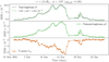 |
Fig. 3. Evolution of intensity of the total brightness B (top panel), polarized brightness pB (mid panel), and F-corona Finv (bottom panel) measured in the pixel (r = 2.6 R⊙, ϕ = 119°) in a sequence of LASCO-C2 images. The dashed green line in the top panel shows the pB profile re-scaled according to the linear model best fitting the B-pB regression (see Fig. 4). The third panel shows the intensity of the F-corona Finv calculated using the inversion method (see Sect. 3.1 for details). The x-axis is in units of days and covers one month (June 2001), whereas the y-axis is in MSB units. The Pearson’s correlation coefficient of the total and polarized brightness (ρB, pB) is equal to 1. |
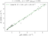 |
Fig. 4. Regression between intensity of total (B) and polarized brightness (pB) obtained in June 2001 at r = 2.6 R⊙ and ϕ = 119° (see also Fig. 3). x and y axes are in MSB units. The dashed green line shows the best fitting linear function. |
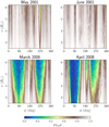 |
Fig. 5. Correlation coefficient m aps obtained for May and June 2001 (solar maximum, top panels) and for March and April 2008 (solar minimum, bottom panels). In all panels the horizontal axis corresponds to the polar angle ϕ in degrees, and the vertical axis is the heliocentric distance r in the R⊙ units. The colors represent the value of the Pearson’s correlation coefficient ρB, pB which ranges between 0 and 1. |
where a and b are constants for a given pixel and considered time interval, which are calculated fitting the corresponding B-pB regression.
On the other hand, the total brightness is equal to the sum of the intensity of the K- and F- coronae:
 (8)
(8)
where we highlighted the time dependence of B and K. We assumed that the typical time scale of the F-corona variations is longer than one month, and, therefore, F can be considered as a constant in our analysis (see e.g., Morgan & Habbal 2007; Llebaria et al. 2021).
We note that the F-corona brightness seen with LASCO evolves with time due to the movement of SOHO on the elliptical orbit, which is also inclined with respect to the plane of symmetry of the inner zodiacal cloud (see detailed discussion in Llebaria et al. 2021). In addition, rotating around the Sun, LASCO observes the F-corona emission originated from different parts of the dust cloud. Using restored F-corona maps provided by Llebaria et al. (2021), we checked that on a one-month timescale such effects introduce intensity variations which are less than ∼1%.
Considering that the polarized brightness pB is a fraction of the K-corona (K = α pB, α ≥ 1), Eq. (8) can be rewritten as follows:
 (9)
(9)
Since B and pB are highly correlated and show a linear relation between each other, we can change the argument in Eq. (9) from time t to intensity pB:
 (10)
(10)
Since the left hand sides of Eqs. (7) and (10) are the same, we can write the following differential equation for α:
 (11)
(11)
Solving it, we obtain the relation between α and pB:
 (12)
(12)
where C is the integration constant. Since pB evolves with time, Eq. (12) represents the time dependence of the parameter α. Additional details and an interpretation of the relation between α, a, and C are provided in Appendix A.
In the particular case when C = 0, α does not depend on time and is equal to a. As follows from Eqs. (3) and (4), this situation is possible when the electron density is changing with time while its spatial distribution remains the same: ne = N(t) f(r). Since the solar corona is constantly rotating, strictly speaking, such a situation can be excluded from our analysis.
In all other cases, C ≠ 0, and the linear relation between B and pB (Eq. (10)) can be rewritten as
 (13)
(13)
Comparing Eqs. (7) and (13), we can conclude that the parameter b obtained from the linear fit is equal to b = C + F. Using only the total and polarized brightness images, it is not possible to disentangle the value of C from F. In order to constrain C and subsequently estimate the intensity of the F-corona, we performed a number of simulations of rotating streamers.
3.2.1. Constraining C by the simulations of the rotating streamer(s)
We performed simulations of non-evolving streamers of conic shape, which rotate solidly with the solar corona in a vacuum environment. The electron density distribution within each streamer was approximated with a power-law function of the cone height nstr ∝ h−5 (adopted from Gibson et al. 1999; Antonucci et al. 2005). It decreases along the height toward the vertex of the cone. The simulations cover 25 days (almost full rotation) with a cadence similar to that of the LASCO-C2 pB observations (three times per day).
For each given pixel of the LASCO-C2 FOV at the projected heliocentric distance x, we determined the radius vectors r1 and r2 from the center of the Sun to the point where the LOS enters and exits a streamer, respectively (see arrows in the bottom right panel of Fig. 6). Projecting vector (r1 − r2) to the height of a streamer, we calculated the relation between nstr and heliocentric distance r. Using the r1 and r2 values as the integration limits in Eqs. (3) and (4), we calculated the Kstr and pBstr intensities:
![Mathematical equation: $$ \begin{aligned} K_{\rm str}(x) = \frac{1}{2} \int _{r_1}^{r_2} n_{\rm str} \left[\left(\frac{2r^2}{x^2} -1\right)A(r) + B(r)\right] \frac{x^2}{r\sqrt{r^2-x^2}} \mathrm{d} r \,, \end{aligned} $$](/articles/aa/full_html/2022/03/aa41414-21/aa41414-21-eq15.gif) (14)
(14)
![Mathematical equation: $$ \begin{aligned} pB_{\rm str}(x) = \frac{1}{2} \int _{r_1}^{r_2} n_{\rm str} \, [A(r) - B(r)] \frac{x^2}{r\sqrt{r^2-x^2}} \mathrm{d} r \, . \end{aligned} $$](/articles/aa/full_html/2022/03/aa41414-21/aa41414-21-eq16.gif) (15)
(15)
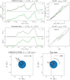 |
Fig. 6. Comparison of variation profiles obtained with observations and simulations. Top panels: variation profiles of B and pB from the LASCO-C2 data (June 2001) and their correlation measured in the pixel at r = 2.8 R⊙ and ϕ = 124°. Mid panels: variation profiles of K and pB and their correlation obtained by the simulation “Sim1” (see Table B.1) at the similar location. The dashed and dotted green lines correspond to the pB profile rescaled according to the linear model best fitting the B-pB and K-pB regressions, respectively. The real and simulated observations cover the time interval of ∼15 days. The simulated intensities are reported in the arbitrary units. Bottom panels: orientation of the two broad simulated streamers at t = 7 days. The position of the pixel of interest is marked with the red dot. X-, Y-, and Z- axes are in the R⊙ units. The gray arrow shows the direction of the solar rotation. The orange arrows in the bottom right panel are the radius vectors r1 and r2 from the center of the Sun to the point where the LOS enters and exits a streamer, respectively (see text for details). |
For simplicity, we omitted the conversion factor Ccf. We also added a factor (1/2) in both equations, since in our simulations the electron density distribution is not symmetric with respect to the POS. We note that if the vector (r1 − r2) intersects the POS, the integrals in Eqs. (14) and (15) are split in two: the first one with the integration limits (x, r1) and the second one with (x, r2). Performing calculations for each moment of time t and for all streamers inside the FOV, we obtained the evolution of K(t) and pB(t).
In order to validate this approach, we compared the evolution of total and polarized brightness extracted from the LASCO-C2 data with K(t) and pB(t) simulated using different number of streamers of various sizes and orientations and considering different pixels within the LASCO-C2 FOV (see Table B.1). Aiming to reproduce the main features seen in the data, we simulated large streamers of ∼6 R⊙ height and ∼10°–20° angular aperture at the vertex. For the particular case of the polar streamer, we simulated a narrow cone with an aperture of 2.5° (see Fig. B.3 and Table B.1). We found that the simulations can reproduce the shape of the variation profiles reasonably well, together with the average slope of the corresponding regression and its correlation coefficient (see some examples in Fig. 6 and Appendix B).
In order to minimize the effect of the solar rotation, we divided the simulated intensity profiles into the overlapping three-day segments and analyzed each segment separately (see Sect. 3.2.2 for details). For segments with the correlation coefficient ρK, pB close to 1 (ρK, pB ≥ 0.85), we fitted the K-pB regression with a linear function fK(pB). Since in our simulations we did not include the contribution from the F-corona, the constant term of fK(pB) corresponds to the parameter C:
 (16)
(16)
We excluded the segments with an average slope of the K-pB regression smaller than 0.95 (a < 0.95) from the analysis. In fact, as follows from Eq. (12), if a is less than 1 the parameter |C| will reach a large value in order to satisfy the condition α ≥ 1. In our procedure, we actually decreased the threshold from 1 to 0.95, aiming to include the segments with low |C|, for which the best fitting parameter a appeared to be close to but smaller than 1 due to the presence of some fluctuations.
Since the simulated intensities are calculated in arbitrary units, we normalized the parameter C to the maximum pB value reached in a segment (pBmax). We then compared the normalized values of C calculated for different segments and simulations and found that in many cases it stays within the range of ±20% of pBmax (see Figs. 7 and 8).
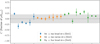 |
Fig. 7. Normalized values of the parameter C obtained by fitting the simulated K-pB regression. Blue, orange, and green colors mark the three-day segments of multi-streamer simulations at intermediate (Int.) and equatorial (Eq.) polar angles, as shown in Figs. 6, B.1, and B.2, respectively. The simulations are labeled as in Table B.1. The error bars represent the best-fitting 1-σ uncertainties. The y-axis shows the values of C as a fraction of pBmax in a segment. The gray shaded area highlights the range of ±20% of pBmax. |
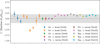 |
Fig. 8. Same as Fig. 7, but for different single-streamer simulations at intermediate (Int.), polar (Pol.), and equatorial (Equ.) polar angles. Each color marks the three-day segments of a specific simulation labeled as in Table B.1. |
Although in the rotating corona the geometry of the electron distribution is constantly changing, in many cases C is close to 0. For example, the simulations of non-equatorial and narrow streamers (with an aperture of ≲10°) provide the best-fitting value of C ≈ 0 and its 1-σ uncertainty of ≲20% of pBmax. Such streamers intersect the LOS in a short time interval, so the variation of α is not large, and, therefore, C is close to 0. The smallest values of |C| are obtained in the polar regions, where the effect of the solar rotation is less significant and the polarized fraction of the K-corona remains rather constant in time (see e.g., purple and brown points in Fig. 8). On the other hand, by simulating equatorial and/or broad streamers, we found that some segments can provide the value of C outside the range of ±20% of pBmax, even when considering the uncertainties.
3.2.2. Estimating the F-corona intensity with the LASCO-C2 data
Similarly to the approach described in Sect. 3.2.1, we divided one-month intensity profiles extracted from the LASCO-C2 data into three-day segments (equivalent to ∼40° of the solar rotation) and analyzed each of them separately. Given a cadence of the pB acquisitions during the chosen months of the LASCO-C2 data set (∼3 times per day), a three-day time interval is sufficiently long for accumulating several measurements and performing an accurate analysis of the B-pB regression. The segments that contain < 4 polarized brightness measurements were not considered in our analysis. By fitting the B-pB regression with a linear function (Eq. (7)), we obtained parameters aseg and bseg for each segment.
We excluded the segments with low correlation ρB, pB < 0.85, since in these cases the linear model does not provide a satisfactory representation of the data. In addition, we excluded the segments with aseg < 0.95, which provide high values of |C| (as explained in Sect. 3.2.1) and, therefore, a biased estimate of F.
As shown in Sect. 3.2.1, if the correlated variations of B and pB seen in a segment are due to the passage of the rotating streamers (as in simulations), the contribution of C is not dominant, and, therefore, the best-fitting parameter bseg can be considered as a reasonable estimate of the intensity of the F-corona. Moreover, if the F-corona is stable on the one-month timescale (as we assumed before), the distribution of bseg values calculated for different segments over one month is expected to have a peak at the value of F. On the other hand, more complicated cases, such as passages of equatorial and/or broad streamers, provide the values of C that deviate significantly from 0. This is expected to cause the broadening of bseg-distribution without shifting the peak.
In our analysis, we considered overlapping segments: the beginning of each segment is shifted by one day with respect to the beginning of the previous segment (i.e., 2 days of overlap). This allowed us to increase the statistics of the bseg-distribution without significantly shifting its peak, since the segments with low correlation and aseg < 0.95 are excluded. In most cases, we obtained the bseg-distribution of a Gaussian shape (see some examples in Fig. 9).
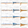 |
Fig. 9. Distribution of bseg values (blue) and that of the F-corona intensity Finv (orange) measured in different pixels in June 2001. The four rows correspond to pixels at r = 2.6 R⊙ and ϕ = 119°, r = 4.5 R⊙ and ϕ = 213°, r = 2.5 R⊙ and ϕ = 0°, and r = 3.5 R⊙ and ϕ = 270° (from top to bottom). Finv is calculated using the inversion method. Left column: evolution of both quantities. Mid and right columns: histogram of the bseg and Finv distributions, respectively. In all panels, the y-axis is in the MSB units. The red and green solid lines show the Gaussian fits of the bseg and Finv distributions, respectively. The mean and standard deviation of these distributions are shown by means of the blue dashed and orange dotted lines with the corresponding shaded area, respectively. The upper limit of the F-corona intensity and the estimate of its systematic uncertainty inferred from the correlation method are shown for each segment as the blue arrow and the error bar, respectively (see text for details). |
The intensity of the F-corona (Fcorr) was calculated as the mean value of bseg-distribution. The corresponding statistical uncertainty (σstat, corr) was estimated as the spread of bseg values (standard deviation). We also calculated the systematic uncertainty on Fcorr caused by the lack of knowledge of the parameter C. We assumed that 20% of pBmax in each segment can be considered as a reasonable estimate of the systematic uncertainty of the F-corona intensity. The final systematic uncertainty on Fcorr (σsys, corr) is obtained by averaging the systematic uncertainties of all segments. Finally, we calculated an upper limit of the F-corona intensity equal to (B-pB), and checked that the estimated value of Fcorr satisfies this limit both during each single segment and the whole month.
4. Results
4.1. F-corona images
We repeated the procedure described in Sect. 3.2.2 for every pixel of the LASCO-C2 images and obtained the F-corona (Fcorr) intensity maps for two months during the solar maximum (May and June 2001) and two months during the solar minimum (March and April 2008). We calculated the maps that represent the relative statistical and systematic uncertainties on Fcorr. Both quantities typically do not exceed 10–15%. Resulting maps are shown in Fig. 10. The pixels with no measurement of bseg were left blank. In addition, the pixels of the σstat, corr maps for which the bseg-distribution contains only one measurement were left blank.
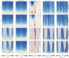 |
Fig. 10. F-corona maps calculated applying the correlation and inversion techniques for different months of data. The four rows correspond to May 2001, June 2001, March 2008, and April 2008 (from top to bottom). First two columns: intensity maps obtained with the correlation method (Fcorr) and the inversion method (Finv). Third column: difference maps (Fcorr − Finv) normalized to the statistical uncertainties on Fcorr (σstat, corr). The relative statistical and systematic uncertainties on Fcorr are shown in the fourth and fifth columns, respectively. In all panels, the horizontal axis corresponds to the polar angle ϕ in degrees, and the vertical axis is the heliocentric distance r in the R⊙ units. The color bars represent the MSB in the first two columns, the σstat, corr in the third column and the fraction of Fcorr in the last two columns. The contour levels (dotted black lines) are reported in the MSB units. Blank pixels colored in gray appear in the regions where the correlation method is not applicable (see text for details). |
We also reconstructed the F-corona maps obtained through the inversion method (Finv) by averaging their evolution over a month and compared them with the Fcorr maps. As shown in Fig. 10, the brightness distribution obtained with the correlation method is smoother and does not contain the oversubtraction/undersubtraction features present in the Finv maps (compare intensity contours in Fig. 10, first and second columns). The most prominent features of Finv maps can be seen in Fig. 10 (second column) at ϕ equal to 0°, 90°, and 180°. We calculated the difference between Fcorr and Finv normalized to the statistical uncertainties on Fcorr (σstat, corr), and we found that in some regions it reaches significant values of up to 5–10 σstat, corr (see Fig. 10, third column). Such a difference is equivalent to ∼10−9 MSB at low heliocentric distances.
Using the F-corona map obtained for June 2001, we reconstructed the image of the K-corona (Kcorr). For this, we subtracted Fcorr from the total brightness image acquired on June 1, 2001 at 09:07. We compared Kcorr with Kinv from Fig. 2, which was obtained using the same B image and the preceding pB image acquired on June 1, 2001 at 9:00. As shown in Fig. 11, the relative difference between these two maps reaches significant values (0.5–5) in the regions where streamers appear.
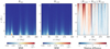 |
Fig. 11. K-corona maps calculated using the inversion (Kinv, left panel) and correlation (Kcorr, mid panel) methods. Kinv is obtained using the pB image acquired on June 1, 2001 at 9:00 and B image on June 1, 2001 at 09:07 (as in Fig. 2). Kcorr is calculated as the difference between the same total brightness image and the Fcorr map obtained for June 2001. Right panel: relative difference between Kcorr and Kinv. The horizontal axis corresponds to the polar angle ϕ in degrees, and the vertical axis is the heliocentric distance r in the R⊙ units. |
We checked whether there is any significant variation of the F-corona intensity from one month to another. The difference maps calculated for two consecutive months (Fig. 12) show that the relative variations are below ∼12% (≲5 × 10⁻¹⁰ MSB), which is within the statistical uncertainties of the Fcorr measurement.
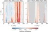 |
Fig. 12. Relative difference between Fcorr maps calculated for two consecutive months. The horizontal axis corresponds to the polar angle ϕ in degrees, and the vertical axis is the heliocentric distance r in the R⊙ units. Blank pixels colored in gray appear in the regions where the correlation method is not applicable (see text for details). |
4.2. Radial profiles of the F-corona
We compared the slope of radial profiles of the F-corona calculated with the correlation and inversion techniques at different polar angles. For this, we fit each profile F(r) with a simple power-law function f(r)∝r−n at r ≥ 3 R⊙. Aiming to achieve a good quality of the fit while maintaining the simplicity of the fitting function, we did not consider the data between 2.5 R⊙ and 3 R⊙ where F(r) changes its slope. The best-fitting exponent n calculated for different months and polar angles is shown in Fig. 13. We did not include the values of n obtained for the polar regions (around 90° and 270°) during the solar minimum. In these quiet regions, less than a half of pixels is defined in the corresponding Fcorr(r) profiles (for a detailed discussion, see Sect. 5.3) and, as a consequence, the best fitting n is not representative.
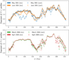 |
Fig. 13. Exponent of radial profiles of the F-corona calculated with the correlation (corr) and inversion (inv) techniques at r ≥ 3 R⊙. Top and bottom panels: values obtained for the solar maximum (May and June 2001) and solar minimum (March and April 2008) months, respectively. The best-fitting 1-σ uncertainties are shown by means of the error bars for the correlation method and the width of shaded areas for the inversion method. |
As can be seen from Fig. 13, both the correlation and inversion methods provide a similar slope of F(r) with n ≈ 2.15 measured along the equator and n ≈ 2.6 along the poles. These estimates are consistent with the values of n derived using the intensity profiles from Saito et al. (1977) and close to those reported in Koutchmy & Lamy (1985) for r ≥ 4 R⊙.
For the solar maximum months, the correlation method provides a smoother relation between n and ϕ than the inversion method, especially at ϕ < 200°. The slopes of the Finv(r) calculated around 90° and 180° for May and June 2001 deviate a lot from each other and from that of Fcorr(r) due to the presence of prominent oversubtraction/undersubtraction features. The relation between n and ϕ calculated for the solar minimum months is rather smooth for all cases, except for the March and April 2008 correlation measurements at ϕ around 200° and 300°, where the F-corona image only partially defined. Finally, we point out that the F-corona profiles at 200° < ϕ < 320° are significantly affected by the contamination from the stray light (see Sect. 5.6 for discussion). The corresponding values of n should be considered as indicative.
5. Discussion
We presented a new correlation method for the direct measurement of the F-corona intensity from the VL data. We showed that the contribution from the F-corona can be reasonably well estimated in regions where the total and polarized brightness are highly correlated without any specific assumption on the geometry of the ne-distribution and/or the polarization of the K-corona.
5.1. Simulation of streamer passages
In order to estimate possible systematic uncertainties of the correlation method, we assumed that time variations of B and pB are mainly caused by passages of streamers which rotate solidly with the Sun. Following this assumption, we simulated how the quantities K and pB vary with time and obtained constraints on the parameter C.
As mentioned in Sect. 3.2.1, the streamers are simulated in the empty environment. However, the presence of electrons outside the streamers can introduce additional shift (dC) of the parameter C, which was not considered in our simulations. Although including this effect is beyond the presentation that we give in this paper, we nonetheless attempted to carry out a rough estimate of dC. For this, we assumed that such an electron population has symmetric density distribution along the line LOS with respect to the POS. Applying the inversion method, we calculated the intensity of the K-corona (Kinv) at the moment of time tmin when the minimum VL brightness is observed during a month. We also assumed that no streamer was passing in front of the observer at tmin. We obtained that the normalized value of |dC| calculated for each pixel of the image as in Eq. (17) does not exceed ∼10% of pBmax:
 (17)
(17)
where a is the best fitting slope of the one-month B-pB regression.
An accurate estimate of dC and C requires a more realistic modeling of the electron density distribution around the Sun (as, e.g., presented in de Patoul et al. 2015). However, our rough estimates suggest that the contribution from dC should not shift the Fcorr intensity calculated with the correlation method dramatically.
5.2. Measuring the intensity of the F-corona
For each pixel, we determined the intensity Fcorr as the mean of bseg-distribution calculated for three-day segments of the VL observations. We compared the distribution of bseg with that of the F-corona intensity (Finv) obtained by applying the inversion method to each pair of pB and B images. A number of the most representative cases are discussed below.
In Fig. 9 (first row), we show both distributions obtained at an intermediate polar angle (ϕ = 119°). The values of bseg are rather stable, whereas the variation profile of Finv is clearly anti-correlated with the B/pB intensity (see also Fig. 3). As mentioned in Sect. 3.1, this happens due to the appearance of the asymmetric structures (such as streamers) in the solar corona during the period from June 7 through June 17, 2001, which leads to the oversubtraction of the K-corona. On the other hand, both methods provide similar estimates of the F-corona intensity outside this time interval, when there was no streamer passing through this region. Taking into account the spread of each distribution, the mean values ⟨bseg⟩ and ⟨Finv⟩ can be considered consistent with each other. We note, however, that ⟨Finv⟩ is lower than ⟨bseg⟩ due to the presence of the above-mentioned underestimated measurements. By removing such measurements from Finv profiles, it is possible to obtain the results closer to those obtained with the correlation method. However, this would require pixel-by-pixel manipulation with the data. An example for which both methods provide similar estimates of the F-corona intensity is shown in Fig. 9 (second row, pixel at ϕ = 213°).
The equatorial and polar cases are shown in the last two rows of Fig. 9. In both examples, Fcorr is higher than ⟨Finv⟩ due to presence of the oversubtraction features. The correlation method (if applicable) provides the most reliable results for the polar regions, where the value of C is close to 0. However, the measurements of Fcorr obtained for the equatorial regions can be affected by the underestimation of the parameter |C|.
The systematic uncertainties on Fcorr defined as 20% of pBmax are comparable with the standard deviation of bseg-distribution (comp. the blue error bars and the blue shaded area in Fig. 9). From this we conclude that the established values of the systematic uncertainties are not underestimated.
5.3. Comparing the F-corona images
Using the correlation method, we obtained the F-corona maps for different months during the solar maximum and solar minimum periods. During solar maxima, the corona is active and it has a lot of streamers appearing at any polar angle. The total and polarized brightness are highly correlated in all regions, so the correlation method can be used for almost all pixels. During periods of minimum, the solar corona is rather quiet with relatively small number of streamers, which are located mainly in the equatorial region. The corresponding F-corona intensity maps have large areas of blank pixels at non-equatorial polar angles where the correlation ρB, pB is low (see Fig. 5). Although in these regions our method is not applicable, the missing values can be calculated by means of the inversion technique. In fact, since there is almost no streamer, the electron density can be considered symmetric, and Finv, therefore, can be considered as a reasonable estimate of F. We calculated the joint F-corona maps (Fjoint) using the correlation and inversion techniques in the high- and low- correlation regions, respectively (see Fig. 14). The intensity contours of the resulting Fjoint maps are rather smooth and do not show a significant step at the boundary of the two applied methods. This suggests that joining the correlation and inversion techniques it is possible to determine the complete F-corona intensity maps during the solar minimum. The final F-corona images converted back to Cartesian coordinates are shown in Fig. 15.
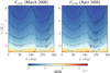 |
Fig. 14. Joint F-corona maps (Fjoint) calculated using the correlation method where applicable and the inversion method otherwise for March 2008 (left panel) and April 2008 (right panel). |
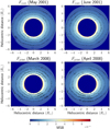 |
Fig. 15. Fcorr and Fjoint maps converted to Cartesian coordinates for May 2001 (top left panel), June 2001 (top right panel), March 2008 (bottom left panel), and April 2008 (bottom right panel). The color bar and contour levels represent the MSB units (as in Figs. 10 and 14). In all panels, both axes correspond to the heliocentric distance in the R⊙ units. |
Compared to the inversion technique, the correlation method is particularly advantageous in the regions where bright streamers appear (especially for the months during the solar maximum). In such regions, the difference between Fcorr and Finv can reach rather significant values up to ∼10−9 MSB. As shown in the difference maps in Fig. 10, for some polar angles (e.g., ϕ ∼ 180°) the electron density profiles ne(r) calculated with the inversion technique provide the overestimated intensity (positive differences) of the K-corona Kinv at all heliocentric distances r from 2.5 to 6.2 R⊙. For other polar angles, for example around 0° and 90°, the ne(r) profiles are such that the resulting intensity Kinv is overestimated at low (r < 3–4 R⊙, positive differences) and underestimated at high (r > 4.5–5 R⊙, negative differences) heliocentric distances. Similar features are present in the difference map of the K-corona (Fig. 11).
5.4. Accounting for the presence of CMEs
Apart from streamers, bright and dynamic K-corona events such as CMEs can cause the variation of the VL brightness. These events evolve much faster than streamers and produce sharp single-point peaks at the variation profiles of the total and polarized brightness (see e.g., a peak on June 20 in Fig. 3). Given the cadence of the pB acquisitions (∼3 images per day) and different orientation of CMEs, each pixel of the pB images converted to polar coordinates detects up to a few bright events (from 0 to ∼3) during a solar maximum month.
Similarly to narrow streamers, CMEs intersect the LOS in a very short time interval, so that in most cases the variation of α is expected to be small, C close to 0, and the corresponding estimate of F unbiased (see Sect. 3.2.1 and Appendix A for details). We found, however, that some CME measurements are outside an average trend of the B-pB regression. This can be caused by the difference between the evolution of the geometry of the electron density distribution within a CME and simultaneously observed streamer(s). For example, if the ejected hot plasma is expanding along the LOS, the polarized fraction of the emitted radiation (and therefore the parameter α) will constantly change and the parameter C will reach significant values. In these cases, the corresponding B-pB measurement can decrease the correlation coefficient of the segment of interest.
The detailed characterization of the parameter α during a CME event is left for future studies. In this work, we estimated an error introduced by the presence of bright CMEs. Since it would be time consuming to manually remove each CME from the data, we implemented the following automatic procedure. Running our analysis, we examined the low correlation segments with ρB, pB < 0.85 and calculated the correlation ρi for each subsample of such a segment by omitting i-th observation. In case the correlation exceeded the threshold ρi ≥ 0.85 for some iteration i, we stored the corresponding best fitting value of bseg and calculated a new value of Fcorr. The difference between new Fcorr maps and those presented above is typically less than ∼0.46 σstat, corr for solar maximum months. During the minimum phase of the solar cycle, CME events appear less frequently, and so the corresponding difference is expected to be even smaller.
5.5. Accounting for the polarization of the F-corona
We estimated the error introduced by neglecting the polarization pF(r) of the F-corona beyond 5 R⊙. Following the model of Blackwell & Petford (1966), we assumed that pF is equal to 0 up to 5 R⊙ and rises from 0.05% at 5 R⊙ to 0.16% at 8 R⊙ as a power-law function: pF ∝ rγ. Taking into account that pB is equal to (pK + pFF) and that the term (pFF) is constant in time, Eqs. (7) and (13) can be rewritten as
 (18)
(18)
 (19)
(19)
Assuming again that the contribution from C is not significant, one can derive that
 (20)
(20)
By adjusting an estimate of F in each three-day segment as shown in Eq. (20), we calculated new values of Fcorr for each pixel at heliocentric distances > 5 R⊙. They differ from Fcorr values presented above by ≲0.13 σstat, corr and ≲0.26 σstat, corr for solar maximum and minimum months, respectively.
5.6. Contamination from the stray light
The F-corona maps presented in this work contain non-negligible contribution from the instrumental stray light. For example, one of its most prominent features arises from the occulter pylon and can be seen as a relatively faint sector at ϕ ≈ 230° (see Fig. 10).
Disentangling the F and stray light components is a nontrivial task, which was beyond the original scope of this paper. Recently, Llebaria et al. (2021) presented the sophisticated procedure for separating these two components from the LASCO-C2 data obtained over 24 years. They used recalibrated total and polarized brightness images (for details, see Lamy et al. 2020) and restored 36 maps that account for the relatively slow temporal variation of the stray light pattern of the LASCO-C2 instrument. We could not use these patterns to remove the stray light from our Fcorr and Finv images, since they were obtained using the data set calibrated in a different way. In order to evaluate the contamination S from the stray light, we repeated our analysis using the newly calibrated total and polarized brightness images stored in the corresponding data archive3, as specified in Lamy et al. (2020), Llebaria et al. (2021). As shown in Fig. 16, the ratio S/F ranges from ∼0 up to 0.5−0.6.
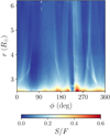 |
Fig. 16. Ratio map (S/F) calculated for June 2001. The stray light pattern S is taken from Llebaria et al. (2021). The F-corona map F is calculated by applying the correlation method to the newly calibrated data presented by Lamy et al. (2020), Llebaria et al. (2021). |
We also found that the recalculated Fcorr maps are consistent with those restored by Llebaria et al. (2021). The relative differences typically do not exceed ∼10–15%, which is comparable with the uncertainties of the correlation method.
6. Conclusions
The correlation method is a new model-independent and data-driven approach for calculating the intensity maps of the F-corona. It provides a more accurate estimate of F than the inversion method in the active regions with streamers and/or CMEs: that is almost the full LASCO-C2 FOV during the solar maximum and about a half of it during the solar minimum. We point out that the correlation method does not require any specific assumption on the geometry of the ne-distribution (as required, e.g., for the inversion technique) and/or a specific model of the K-corona polarization (as required, e.g., for the analysis of Lamy et al. 2020; Llebaria et al. 2021).
We evaluated the uncertainties introduced by not considering the polarization of the F-corona beyond 5 R⊙ and the presence of bright CMEs, and found that they are significantly lower than the statistical errors. As another confirmation of the reliability of the correlation method, we found that it provides results consistent with those of Llebaria et al. (2021), who presented one of the most accurate procedure for the restoration of the F-corona from the LASCO-C2 data. We also obtained that the slope of the radial profiles F(r) calculated at different polar angles is in agreement with the values reported in the literature.
During the periods of solar minimum, our method is not applicable to the quiet polar regions with no streamers. In these parts of the LASCO-C2 FOV the inversion method is expected to provide a reliable estimate of F. Combining the correlation and inversion methods, it is possible to obtain the complete intensity maps of the F-corona during the solar minimum.
Another limitation of the correlation method is that the analyzed data set should cover a certain period of time with a reasonable cadence for measuring the correlation of the total and polarized brightness and determining an accurate estimate of F. As we showed above (e.g., in Fig. 5), one month of data is definitely sufficient to detect the activity in the majority of pixels of the LASCO-C2 FOV during the solar maximum period and in the equatorial pixels during the solar minimum periods. The cadence of ∼3 measurements per day allowed us to achieve an accuracy of about 10–15%. In this respect, the inversion technique is simpler to use, since the Finv map can be derived from a pair of B and pB images. On the other hand, such F-corona images will be distorted by the oversubtraction/undersubtraction features even more than the monthly averaged Finv maps shown in Fig. 10.
Resulting Fcorr maps can be used for reconstructing accurate images of the K-corona, which is necessary to characterize the electron population within the solar corona. By applying the correlation method to larger data sets, it will be possible to analyze the time evolution of the F-corona brightness distribution observed with LASCO. Our method does not allow us to separate the contribution of the stray light from the F-corona. For this purpose, one can use the stray light patterns obtained by means of other techniques. Once corrected for the presence of the stray light, accurate Fcorr images can be used for studying the distribution of the interplanetary dust.
Although the correlation method already provides reliable results, a number of further steps can be taken to improve it:
-
By developing more realistic simulations, it will be possible to establish more accurate constraints on C and to decrease the corresponding systematic uncertainties on F. For example, one can consider more complex shapes of a streamer with the orientation evolving with time. Including a population of electrons outside the streamers, we will be able to evaluate dC directly from the simulations.
-
The detailed investigation of the passages of equatorial and/or broad streamers is necessary for providing a more reliable estimate of the F-corona intensity for these cases.
-
By investigating the variation of the polarized fraction of the K-corona (equiv. to 1/α) during the CME events, it will be possible to explain the presence of the CME measurements that are outside an average trend of the B-pB regression. Carefully removing such measurements from the data will allow us to improve an accuracy of the Fcorr maps.
-
Additional improvements can be achieved accounting for the polarization of the F-corona above several R⊙.
With the high-cadence pB observations, it will be possible to obtain a more accurate measurement of F, decreasing both the statistical and the systematic uncertainties. Such observations will be carried out in the near future with the Metis instrument (Antonucci et al. 2020) – a coronagraph onboard the Solar Orbiter mission (García Marirrodriga et al. 2021) that is currently in the cruise phase. In contrast to LASCO, Metis is going to acquire both the total and polarized brightness images during each VL observation, providing more frequent series of images for the correlation analysis. In addition, the out-of-ecliptic observations of Metis will allow us to obtain the longitudinal brightness distribution of the F-corona for the first time.
Acknowledgments
We thank the referee for his/her in-depth comments. A.B. would like to thank Dr. Polina Zemko for very useful discussions and suggestions. This activity has been supported by ASI and INAF under the contract: Accordo ASI-INAF & Addendum N. I-013-12-0/1. In this work we made use of the following Python packages: Matplotlib (Hunter 2007), NumPy (Harris et al. 2020), SciPy (Virtanen et al. 2020), Astropy (Astropy Collaboration 2013, 2018). This work makes use of the LASCO-C2 legacy archive data produced by the LASCO-C2 team at the Laboratoire d’Astrophysique de Marseille and the Laboratoire Atmosphères, Milieux, Observations Spatiales, both funded by the Centre National d’Etudes Spatiales (CNES). LASCO was built by a consortium of the Naval Research Laboratory, USA, the Laboratoire d’Astrophysique de Marseille (formerly Laboratoire d’Astronomie Spatiale), France, the Max-Planck-Institut für Sonnensystemforschung (formerly Max Planck Institute für Aeronomie), Germany, and the School of Physics and Astronomy, University of Birmingham, UK. SOHO is a project of international cooperation between ESA and NASA.
References
- Antonucci, E., Abbo, L., & Dodero, M. A. 2005, A&A, 435, 699 [NASA ADS] [CrossRef] [EDP Sciences] [Google Scholar]
- Antonucci, E., Romoli, M., Andretta, V., et al. 2020, A&A, 642, A10 [NASA ADS] [CrossRef] [EDP Sciences] [Google Scholar]
- Astropy Collaboration (Robitaille, T. P., et al.) 2013, A&A, 558, A33 [NASA ADS] [CrossRef] [EDP Sciences] [Google Scholar]
- Astropy Collaboration (Price-Whelan, A. M., et al.) 2018, AJ, 156, 123 [Google Scholar]
- Blackwell, D. E., & Petford, A. D. 1966, MNRAS, 131, 399 [NASA ADS] [CrossRef] [Google Scholar]
- Boe, B., Habbal, S., Downs, C., & Druckmüller, M. 2021, ApJ, 912, 44 [NASA ADS] [CrossRef] [Google Scholar]
- Brueckner, G. E., Howard, R. A., Koomen, M. J., et al. 1995, Sol. Phys., 162, 357 [NASA ADS] [CrossRef] [Google Scholar]
- de Patoul, J., Foullon, C., & Riley, P. 2015, ApJ, 814, 68 [NASA ADS] [CrossRef] [Google Scholar]
- Dolei, S., Spadaro, D., & Ventura, R. 2015, A&A, 577, A34 [NASA ADS] [CrossRef] [EDP Sciences] [Google Scholar]
- Domingo, V., Fleck, B., & Poland, A. I. 1995, Sol. Phys., 162, 1 [Google Scholar]
- Freeland, S. L., & Handy, B. N. 1998, Sol. Phys., 182, 497 [Google Scholar]
- García Marirrodriga, C., Pacros, A., Strandmoe, S., et al. 2021, A&A, 646, A121 [CrossRef] [EDP Sciences] [Google Scholar]
- Gibson, S. E., Fludra, A., Bagenal, F., et al. 1999, J. Geophys. Res., 104, 9691 [Google Scholar]
- Harris, C. R., Millman, K. J., van der Walt, S. J., et al. 2020, Nature, 585, 357 [NASA ADS] [CrossRef] [Google Scholar]
- Hayes, A. P., Vourlidas, A., & Howard, R. A. 2001, ApJ, 548, 1081 [Google Scholar]
- Howard, R. A., Vourlidas, A., Bothmer, V., et al. 2019, Nature, 576, 232 [Google Scholar]
- Hunter, J. D. 2007, Comput. Sci. Eng., 9, 90 [NASA ADS] [CrossRef] [Google Scholar]
- Koutchmy, S., & Lamy, P. L. 1985, The F-Corona and the Circum-Solar Dust Evidences and Properties (ir), ed. S. Koutchmy, 63 [Google Scholar]
- Lamy, P., Quemerais, E., Llebaria, A., et al. 1997, in Fifth SOHO Workshop: The Corona and Solar Wind Near Minimum Activity, ed. A. Wilson, ESA Spec. Publ., 404, 491 [NASA ADS] [Google Scholar]
- Lamy, P., Llebaria, A., Boclet, B., et al. 2020, Sol. Phys., 295, 89 [CrossRef] [Google Scholar]
- Lamy, P., Gilardy, H., Llebaria, A., Quémerais, E., & Ernandez, F. 2021, Sol. Phys., 296, 76 [NASA ADS] [CrossRef] [Google Scholar]
- Llebaria, A., Lamy, P., Gilardy, H., Boclet, B., & Loirat, J. 2021, Sol. Phys., 296, 53 [NASA ADS] [CrossRef] [Google Scholar]
- Minnaert, M. 1930, ZAp, 1, 209 [NASA ADS] [Google Scholar]
- Morgan, H., & Habbal, S. R. 2007, A&A, 471, L47 [NASA ADS] [CrossRef] [EDP Sciences] [Google Scholar]
- Morgan, H., & Habbal, S. 2010, ApJ, 711, 631 [NASA ADS] [CrossRef] [Google Scholar]
- Morrill, J. S., Korendyke, C. M., Brueckner, G. E., et al. 2006, Sol. Phys., 233, 331 [NASA ADS] [CrossRef] [Google Scholar]
- Quémerais, E., & Lamy, P. 2002, A&A, 393, 295 [NASA ADS] [CrossRef] [EDP Sciences] [Google Scholar]
- Ragot, B. R., & Kahler, S. W. 2003, ApJ, 594, 1049 [NASA ADS] [CrossRef] [Google Scholar]
- Saito, K., Poland, A. I., & Munro, R. H. 1977, Sol. Phys., 55, 121 [NASA ADS] [CrossRef] [Google Scholar]
- Stauffer, J. R., Stenborg, G., & Howard, R. A. 2018, ApJ, 864, 29 [NASA ADS] [CrossRef] [Google Scholar]
- Stenborg, G., & Howard, R. A. 2017, ApJ, 839, 68 [Google Scholar]
- van de Hulst, H. C. 1950, Bull. Astron. Inst. Neth., 11, 135 [Google Scholar]
- Virtanen, P., Gommers, R., Oliphant, T. E., et al. 2020, Nat. Methods, 17, 261 [Google Scholar]
Appendix A: Deriving the relation between the parameters α, a, and C
Assuming that pB0 is the polarized brightness at time t0 and that α0 = α(pB0) as boundary conditions, we integrated the differential Eq. (11) and obtained the following:
 (A.1)
(A.1)
or, alternatively,
 (A.2)
(A.2)
From Eq. (A.2), we derived the solution of the differential equation in a general form:
 (A.3)
(A.3)
The simplified form of this equation was obtained assigning the expression pB0 (α0 − a) to the parameter C (see Eq. (12)). In addition, from Eq. (A.3) we can find that
 (A.4)
(A.4)
and
 (A.5)
(A.5)
In Fig. A.1, we show a schematic plot with two measurements of K and pB performed in close moments of time (t0 and t1). The linear function which passes thorough both points is given by Eq. (A.4), and has a slope equal to a, as can easily be derived from Eq. (A.5). It intersects the y-axis (pB = 0) at the value equal to C (see Eq. (A.4)). The parameter C can thus be interpreted as the value reached by intensity K when its polarized fraction is equal to 0 and the slope of the K-pB regression is equal to a.
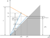 |
Fig. A.1. Two consecutive measurements of K and pB at time t0 and t1 (black dots). The orange solid line with a slope equal to a passes through both points and intersects the y-axis at K = C. Since K ≥ pB, no (pB, K)-point can appear within the gray shaded area below the line K = pB with a slope equal to 1. Kunpol corresponds to the unpolarized fraction of the intensity K. |
The total brightness images contain the contribution from both the K- and F- coronae, and, as mentioned in Sect. 3.2, the parameters C and F cannot be derived from the linear fit of the B-pB regression. In fact, the constant term b of the best-fitting function can, in principle, provide either an unbiased estimate of the F-corona intensity (if C = 0), an overestimated value of F (if C > 0), or, alternatively, an underestimated value of F (if C < 0). The schematic representation of these three cases is shown in Fig. A.2.
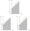 |
Fig. A.2. Linear function (orange line) fit to the pB, B-measurements (black dots). Three panels represent the cases when the best-fitting parameter b provides an unbiased estimate of the F-corona intensity F (top left panel, C = 0), an overestimated value of F (top right panel, C > 0), and an underestimated value of F (bottom panel, C < 0). Since K ≥ pB, no (pB, B)-point can appear within the gray shaded area below the line B = pB + F with a slope equal to 1. |
Appendix B: Details on the streamer simulations
We simulated the non-evolving streamers that rotate solidly with the Sun and calculated the evolution of K(t) and pB(t) intensities as explained in Sect. 3.2.1. In our simulations, we considered different numbers of streamers of various sizes and orientations, as well as different pixels within the LASCO-C2 FOV. We compared the evolution of B and pB brightness extracted from the LASCO-C2 data with K(t) and pB(t) simulated for different cases listed in Table B.1. Some examples are shown in Figs. B.1-B.3.
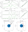 |
Fig. B.1. Same as Fig. 6, but for the pixel at r = 3.5 R⊙ and ϕ ≈ 50° (May 2001). Bottom panels represent the orientation of two narrow simulated streamers at t = 9.33 days, as defined in Table B.1 (“Sim2”). |
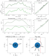 |
Fig. B.2. Same as Fig. 6, but for the pixel at r = 2.8 R⊙ and ϕ ≈ 10° (March 2008). Bottom panels represent the orientation of four broad simulated streamers at t = 1 days, as defined in Table B.1 (“Sim3”). |
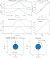 |
Fig. B.3. Same as Fig. 6, but for the pixel at r = 3.1 R⊙ and ϕ ≈ 90° (May 2001). The real and simulated data cover the time interval of ∼4 days. Bottom panels represent the orientation of a narrow simulated streamer at t = 4 days, as defined in Table B.1 (“Sim8”). |
Summary of the simulated configurations of streamers.
All Tables
All Figures
|
Fig. 1. Illustration of the geometry used in the inversion technique. The origin of the coordinate system (O) is placed at the center of the Sun. The pixel of interest P is in the plane of sky YOZ. The line of sight (LOS) parallel to the OX-axis is shown as the red arrow. The OZ-axis points to the north pole of the Sun |
| In the text | |
|
Fig. 2. Polarized (pB, top left panel) and total (B, top mid panel) brightness images obtained with LASCO-C2. pB image was acquired on June 1, 2001 at 9:00, whereas the B image was acquired on June 1, 2001 at 09:07. The electron density ne (bottom left panel), K-corona Kinv (bottom mid panel) and F-corona Finv maps (right panels) are calculated using the inversion technique (see Sect. 3.1). Finv is shown in polar and Cartesian coordinates. The horizontal axis corresponds to the polar angle ϕ in degrees, whereas the vertical axis is the heliocentric distance r in the R⊙ units in all panels except the bottom right, for which both axes correspond to the heliocentric distance. The color bar represents the intensity in MSB units in all panels except the ne map, for which it represents the density in cm−3 units. |
| In the text | |
|
Fig. 3. Evolution of intensity of the total brightness B (top panel), polarized brightness pB (mid panel), and F-corona Finv (bottom panel) measured in the pixel (r = 2.6 R⊙, ϕ = 119°) in a sequence of LASCO-C2 images. The dashed green line in the top panel shows the pB profile re-scaled according to the linear model best fitting the B-pB regression (see Fig. 4). The third panel shows the intensity of the F-corona Finv calculated using the inversion method (see Sect. 3.1 for details). The x-axis is in units of days and covers one month (June 2001), whereas the y-axis is in MSB units. The Pearson’s correlation coefficient of the total and polarized brightness (ρB, pB) is equal to 1. |
| In the text | |
|
Fig. 4. Regression between intensity of total (B) and polarized brightness (pB) obtained in June 2001 at r = 2.6 R⊙ and ϕ = 119° (see also Fig. 3). x and y axes are in MSB units. The dashed green line shows the best fitting linear function. |
| In the text | |
|
Fig. 5. Correlation coefficient m aps obtained for May and June 2001 (solar maximum, top panels) and for March and April 2008 (solar minimum, bottom panels). In all panels the horizontal axis corresponds to the polar angle ϕ in degrees, and the vertical axis is the heliocentric distance r in the R⊙ units. The colors represent the value of the Pearson’s correlation coefficient ρB, pB which ranges between 0 and 1. |
| In the text | |
|
Fig. 6. Comparison of variation profiles obtained with observations and simulations. Top panels: variation profiles of B and pB from the LASCO-C2 data (June 2001) and their correlation measured in the pixel at r = 2.8 R⊙ and ϕ = 124°. Mid panels: variation profiles of K and pB and their correlation obtained by the simulation “Sim1” (see Table B.1) at the similar location. The dashed and dotted green lines correspond to the pB profile rescaled according to the linear model best fitting the B-pB and K-pB regressions, respectively. The real and simulated observations cover the time interval of ∼15 days. The simulated intensities are reported in the arbitrary units. Bottom panels: orientation of the two broad simulated streamers at t = 7 days. The position of the pixel of interest is marked with the red dot. X-, Y-, and Z- axes are in the R⊙ units. The gray arrow shows the direction of the solar rotation. The orange arrows in the bottom right panel are the radius vectors r1 and r2 from the center of the Sun to the point where the LOS enters and exits a streamer, respectively (see text for details). |
| In the text | |
|
Fig. 7. Normalized values of the parameter C obtained by fitting the simulated K-pB regression. Blue, orange, and green colors mark the three-day segments of multi-streamer simulations at intermediate (Int.) and equatorial (Eq.) polar angles, as shown in Figs. 6, B.1, and B.2, respectively. The simulations are labeled as in Table B.1. The error bars represent the best-fitting 1-σ uncertainties. The y-axis shows the values of C as a fraction of pBmax in a segment. The gray shaded area highlights the range of ±20% of pBmax. |
| In the text | |
|
Fig. 8. Same as Fig. 7, but for different single-streamer simulations at intermediate (Int.), polar (Pol.), and equatorial (Equ.) polar angles. Each color marks the three-day segments of a specific simulation labeled as in Table B.1. |
| In the text | |
|
Fig. 9. Distribution of bseg values (blue) and that of the F-corona intensity Finv (orange) measured in different pixels in June 2001. The four rows correspond to pixels at r = 2.6 R⊙ and ϕ = 119°, r = 4.5 R⊙ and ϕ = 213°, r = 2.5 R⊙ and ϕ = 0°, and r = 3.5 R⊙ and ϕ = 270° (from top to bottom). Finv is calculated using the inversion method. Left column: evolution of both quantities. Mid and right columns: histogram of the bseg and Finv distributions, respectively. In all panels, the y-axis is in the MSB units. The red and green solid lines show the Gaussian fits of the bseg and Finv distributions, respectively. The mean and standard deviation of these distributions are shown by means of the blue dashed and orange dotted lines with the corresponding shaded area, respectively. The upper limit of the F-corona intensity and the estimate of its systematic uncertainty inferred from the correlation method are shown for each segment as the blue arrow and the error bar, respectively (see text for details). |
| In the text | |
|
Fig. 10. F-corona maps calculated applying the correlation and inversion techniques for different months of data. The four rows correspond to May 2001, June 2001, March 2008, and April 2008 (from top to bottom). First two columns: intensity maps obtained with the correlation method (Fcorr) and the inversion method (Finv). Third column: difference maps (Fcorr − Finv) normalized to the statistical uncertainties on Fcorr (σstat, corr). The relative statistical and systematic uncertainties on Fcorr are shown in the fourth and fifth columns, respectively. In all panels, the horizontal axis corresponds to the polar angle ϕ in degrees, and the vertical axis is the heliocentric distance r in the R⊙ units. The color bars represent the MSB in the first two columns, the σstat, corr in the third column and the fraction of Fcorr in the last two columns. The contour levels (dotted black lines) are reported in the MSB units. Blank pixels colored in gray appear in the regions where the correlation method is not applicable (see text for details). |
| In the text | |
|
Fig. 11. K-corona maps calculated using the inversion (Kinv, left panel) and correlation (Kcorr, mid panel) methods. Kinv is obtained using the pB image acquired on June 1, 2001 at 9:00 and B image on June 1, 2001 at 09:07 (as in Fig. 2). Kcorr is calculated as the difference between the same total brightness image and the Fcorr map obtained for June 2001. Right panel: relative difference between Kcorr and Kinv. The horizontal axis corresponds to the polar angle ϕ in degrees, and the vertical axis is the heliocentric distance r in the R⊙ units. |
| In the text | |
|
Fig. 12. Relative difference between Fcorr maps calculated for two consecutive months. The horizontal axis corresponds to the polar angle ϕ in degrees, and the vertical axis is the heliocentric distance r in the R⊙ units. Blank pixels colored in gray appear in the regions where the correlation method is not applicable (see text for details). |
| In the text | |
|
Fig. 13. Exponent of radial profiles of the F-corona calculated with the correlation (corr) and inversion (inv) techniques at r ≥ 3 R⊙. Top and bottom panels: values obtained for the solar maximum (May and June 2001) and solar minimum (March and April 2008) months, respectively. The best-fitting 1-σ uncertainties are shown by means of the error bars for the correlation method and the width of shaded areas for the inversion method. |
| In the text | |
|
Fig. 14. Joint F-corona maps (Fjoint) calculated using the correlation method where applicable and the inversion method otherwise for March 2008 (left panel) and April 2008 (right panel). |
| In the text | |
|
Fig. 15. Fcorr and Fjoint maps converted to Cartesian coordinates for May 2001 (top left panel), June 2001 (top right panel), March 2008 (bottom left panel), and April 2008 (bottom right panel). The color bar and contour levels represent the MSB units (as in Figs. 10 and 14). In all panels, both axes correspond to the heliocentric distance in the R⊙ units. |
| In the text | |
|
Fig. 16. Ratio map (S/F) calculated for June 2001. The stray light pattern S is taken from Llebaria et al. (2021). The F-corona map F is calculated by applying the correlation method to the newly calibrated data presented by Lamy et al. (2020), Llebaria et al. (2021). |
| In the text | |
|
Fig. A.1. Two consecutive measurements of K and pB at time t0 and t1 (black dots). The orange solid line with a slope equal to a passes through both points and intersects the y-axis at K = C. Since K ≥ pB, no (pB, K)-point can appear within the gray shaded area below the line K = pB with a slope equal to 1. Kunpol corresponds to the unpolarized fraction of the intensity K. |
| In the text | |
|
Fig. A.2. Linear function (orange line) fit to the pB, B-measurements (black dots). Three panels represent the cases when the best-fitting parameter b provides an unbiased estimate of the F-corona intensity F (top left panel, C = 0), an overestimated value of F (top right panel, C > 0), and an underestimated value of F (bottom panel, C < 0). Since K ≥ pB, no (pB, B)-point can appear within the gray shaded area below the line B = pB + F with a slope equal to 1. |
| In the text | |
|
Fig. B.1. Same as Fig. 6, but for the pixel at r = 3.5 R⊙ and ϕ ≈ 50° (May 2001). Bottom panels represent the orientation of two narrow simulated streamers at t = 9.33 days, as defined in Table B.1 (“Sim2”). |
| In the text | |
|
Fig. B.2. Same as Fig. 6, but for the pixel at r = 2.8 R⊙ and ϕ ≈ 10° (March 2008). Bottom panels represent the orientation of four broad simulated streamers at t = 1 days, as defined in Table B.1 (“Sim3”). |
| In the text | |
|
Fig. B.3. Same as Fig. 6, but for the pixel at r = 3.1 R⊙ and ϕ ≈ 90° (May 2001). The real and simulated data cover the time interval of ∼4 days. Bottom panels represent the orientation of a narrow simulated streamer at t = 4 days, as defined in Table B.1 (“Sim8”). |
| In the text | |
Current usage metrics show cumulative count of Article Views (full-text article views including HTML views, PDF and ePub downloads, according to the available data) and Abstracts Views on Vision4Press platform.
Data correspond to usage on the plateform after 2015. The current usage metrics is available 48-96 hours after online publication and is updated daily on week days.
Initial download of the metrics may take a while.