| Issue |
A&A
Volume 659, March 2022
|
|
|---|---|---|
| Article Number | A10 | |
| Number of page(s) | 29 | |
| Section | Planets and planetary systems | |
| DOI | https://doi.org/10.1051/0004-6361/202141181 | |
| Published online | 25 February 2022 | |
MHD study of the planetary magnetospheric response during extreme solar wind conditions: Earth and exoplanet magnetospheres applications
1
Universidad Carlos III de Madrid,
Leganes,
28911,
Spain
e-mail: jvrodrig@fis.uc3m.es
2
Laboratoire AIM, CEA/DRF – CNRS – Univ. Paris Diderot – IRFU/DAp, Paris-Saclay,
91191
Gif-sur-Yvette Cedex,
France
3
IRAP, Université Toulouse III–Paul Sabatier, CNRS, CNES,
Toulouse,
France
4
LESIA & USN, Observatoire de Paris, CNRS, PSL/SU/UPMC/UPD/UO,
Place J. Janssen,
92195
Meudon,
France
5
LESIA, Observatoire de Paris, Université PSL, CNRS, Sorbonne Université, Université de Paris,
5 place Jules Janssen,
92195
Meudon,
France
Received:
26
April
2021
Accepted:
11
October
2021
Context. The stellar wind and the interplanetary magnetic field modify the topology of planetary magnetospheres. Consequently, the hazardous effect of the direct exposition to the stellar wind, for example, regarding the integrity of satellites orbiting the Earth or the habitability of exoplanets, depends upon the space weather conditions.
Aims. The aim of the study is to analyze the response of an Earth-like magnetosphere for various space weather conditions and interplanetary coronal mass ejections. The magnetopause standoff distance, the open-close field line boundary, and plasma flows toward the planet surface are calculated.
Methods. We used the magnetohydrodynamics code PLUTO in spherical coordinates to perform a parametric study of the dynamic pressure and temperature of the stellar wind as well as of the interplanetary magnetic field intensity and orientation. The range of the parameters we analyzed extends from regular to extreme space weather conditions, which is consistent with coronal mass ejections at the Earth orbit for the present and early periods of the solar main sequence. In addition, implications of sub-Afvénic solar wind configurations for the Earth and exoplanet magnetospheres were analyzed.
Results. The direct precipitation of the solar wind at the Earth dayside in equatorial latitudes is extremely unlikely even during super coronal mass ejections. On the other hand, for early evolution phases during the solar main sequence, when the solar rotation rate was at least five times faster (<440 Myr), the Earth surface was directly exposed to the solar wind during coronal mass ejections. Today, satellites at high, geosynchronous, and medium orbits are directly exposed to the solar wind during coronal mass ejections because part of the orbit at the Earth dayside is beyond the nose of the bow shock.
Key words: magnetohydrodynamics (MHD) / Earth / planets and satellites: magnetic fields
© ESO 2022
1 Introduction
Space weather forecasting in the past decades has shown the important effect of the solar wind (SW) and interplanetary magnetic field (IMF) on the state of Earth’s magnetosphere, ionosphere, thermosphere, and exosphere (Poppe & Jorden 2006; González Hernández et al. 2014). Physical phenomena such as geomagnetic storms (Gonzalez et al. 1994) and substorms (Baker et al. 1999), the energization of the Van Allen radiation belts (Shah et al. 2016), ionospheric disturbances (Cherniak & Zakharenkova 2018), aurorae (Zhang & Paxton 2016), and geomagnetically induced currents at Earth’s surface (Pulkkinen et al. 2017) are triggered during particular space weather conditions. Extreme space weather conditions linked to coronary mass ejections (CME) lead to a strong perturbation of the Earth’s magnetosphere (Cane et al. 2000; Richardson et al. 2001; Wang et al. 2003b; Lugaz et al. 2015; Wu & Lepping 2015). The list of consequences is long: failure of spacecraft electronics due to radiation damage and charging (Choi et al. 2011), enhancement of the drag on low-orbit satellites (Nwankwo et al. 2015), spacecraft signal scintillation due to a perturbed ionosphere (Molera Calvés et al. 2014), ground-induced electric currents that can cause the collapse of electric power grids (Cannon et al. 2013), and ionizing radiation that harms astronauts and passengers of the commercial aviation (Bazilevskaya 2005), among others. Recently, the analysis of the space weather has been generalized for the case of stars different than the Sun (Strugarek et al. 2015; Garraffo et al. 2016). Among other factors, the habitability of exoplanets depends on the space weather conditions imposed by the hosting star and the shielding efficiency of the exoplanet magnetic field, avoiding the sterilizing effect of the stellar wind on the planet surface (Gallet et al. 2017; Linsky 2019; Airapetian et al. 2020). In addition, the direct exposition of the exoplanet to the stellar wind leads to the depletion of the atmosphere, particularly, of volatile molecules such as water by thermal and nonthermal escape (Lundin et al. 2007; Moore & Khazanov 2010; Jakosky et al. 2015).
The CMEs are solar eruptions caused by magnetic reconnections in the star corona (Low 2001; Howard 2006). They expel a large amount of fast charged particles and a magnetic cloud that evolves into an interplanetary coronal mass ejection (ICME; Sheeley Jr. et al. 1985; Neugebauer & Goldstein 1997; Cane & Richardson 2003; Gosling 1990). If the ICME impacts the Earth, the measured SW dynamic pressure increases to 10−100 nPa and the IMF intensity to 100–300 nT (Gosling et al. 1991; Huttunen et al. 2002; Manchester IV et al. 2004; Schwenn et al. 2005; Riley 2012; Howard 2014; Mays et al. 2015; Kay et al. 2017; Savani et al. 2017; Salman et al. 2018; Kilpua et al. 2019; Hapgood 2019). The Disturbance Storm Time Index (Dst) indicates the magnetic activity derived from a network of near-equatorial geomagnetic observatories that measures the intensity of the globally symmetrical equatorial electrojet (the ring current), which is widely used to identify extreme SW and IMF space weather conditions (Sugiura & Chapman 1960; Loewe & Prölss 1997; Siscoe et al. 2006; Borovsky & Shprits, Yuri 2017). A negative Dst value means that Earth’s magnetic field is weakened due to the IMF erosion, particularly during solar storms. The strongest event observed so far is the Carrington event that occurred in 1859 (Carrington 1859). An unusual large number of sunspots on the solar disk and a wide active region was registered, and an extremely fast ICME was launched from it toward the Earth. Several authors studied the Carrington event and suggested that it was a shock that traveled at about 2000 km s−1 (Cliver et al. 1990) that generated the strongest geomagnetic storm with Dst ≈−1700 nT (Tsurutani et al. 2003). This was later revised to Dst ≈−850 nT by Siscoe et al. (2006). The most recent strongest event, called the Bastille Day event (14–16 July 2000), reached a Dst ≈−300 nT for an SW velocity of 1000 km s−1 and an IMF intensity of ≈45 nT (Rastatter et al. 2002). On the other hand, typical ICMEs impacting the Earth show an averaged plasma velocity of 350–500 km s−1 and IMF intensities between 9–13 nT, leading to geomagnetic storms with Dst < −50 nT (Cane & Richardson 2003).
The interaction of the SW with planetary magnetospheres can be studied using numerical models. Different computational frameworks were used, for example, single fluid (Kabin et al. 2008; Jia et al. 2015; Strugarek et al. 2014, 2015), multifluid (Kidder et al. 2008), and hydrid codes (Wang et al. 2010; Müller et al. 2011, 2012; Richer et al. 2012; Turc et al. 2015). The simulations indicate a stronger compression of the bow shock as the SW dynamic pressure increases, as well as an enhancement or a weakening of the effective planet magnetic field according to the IMF orientation and intensity, leading to a modification of the magnetosphere topology (Slavin & Holzer 1979; Kabin et al. 2000; Slavin et al. 2009). Regarding the Earth magnetosphere, several magnetohydrodynamics (MHD) models were developed to analyze the interaction of the Earth magnetic field with the SW and IMF: the GEDAS model (Ogino et al. 1994), the Tanaka model (Tanaka 1994), the block-adaptive tree solar-wind Roe-type upwind scheme (BATS-R-US; Powell et al. 1999), the grand unified magnetosphere-ionosphere coupling simulation, version 4 (Janhunen et al. 2012), the Lyon-Fedder-Mobarry (LFM) model (Lyon et al. 2004), the space weather modeling framework (SWMF; Tóth et al. 2005), the open general geospace circulation model (OpenGGCM; Raeder 2003), the piecewise parabolic method with a Lagrangian remap MHD (PPMLR-MHD) model (Hu et al. 2005), and the adaptive mesh refinement conservation element and solution element AMR-CESE-MHD model (Wang et al. 2015). Thus, the effect of different SW and IMF configurations on the global structures of the Earth magnetosphere has been analyzed by several authors using MHD codes, particularly the bow shock (Samsonov et al. 2007; Andréeová et al. 2008; Nouzák et al. 2011; Mejnertsen et al. 2018), the magnetosheath (Ogino et al. 1992; Wang et al. 2004), the magnetopause standoff distance (Cairns & Lyon 1995, 1996; Wang et al. 2012), and the magnetotail (Laitinen et al. 2005; Wang et al. 2014). In addition, global MHD models were applied to analyze the interaction of ICMEs with the Earth magnetosphere (Wu & Lepping 2002; Wu et al. 2006, 2016; Shen et al. 2011; Ngwira et al. 2013; Scolini et al. 2018; Torök et al. 2018). The simulations show large topological deformations caused by the combined effect of the SW dynamic pressure, IMF magnetic pressure, and the reconnection between the IMF and the Earth magnetic field. Consequently, the magnetopause standoff distance significantly decreases (Sibeck et al. 1991; Dusik et al. 2010; Liu et al. 2015; Nouzák et al. 2016; Grygorov et al. 2017; Samsonov et al. 2020).
Magnetohydrodynamics codes were validated by comparing the simulation results with ground-based magnetometers and spacecraft measurements (Watanabe & Sato 1990). For example, Raeder et al. (2001) compared global Earth magnetosphere simulations with magnetometer and plasma data obtained from spacecrafts during the substorm event of 24∕11∕1996 (dd, month, yyyy). Wang et al. (2003a) calculated the plasma depletion layer and compared the results with Wind satellite data. Den et al. (2006) developed a real-time Earth magnetosphere simulator using the data measured from the spacecraft ACE. These data were compared with geomagnetic field activities as well as with real-time plasma temperature and density data at the geostationary orbit. Facskó et al. (2016) performed a one-year global simulation of the Earth’s magnetosphere comparing the results with CLUSTER spacecraft measurements. In addition, predictions of BATS-R-US, the GUMICS, the LFM, and the OpenGGCM in Honkonen et al. (2013) were compared with measurements of the Cluster (Escoubet et al. 2001), Wind (Acuña et al. 1995), and GEOTAIL (Nishida et al. 1992) missions, as well as with the Super Dual Auroral Radar Network (SuperDARN; Greenwald et al. 1995) cross polar cap potential (CPCP).
The aim of this study is to analyze the topology of the Earth magnetosphere and that of exoplanets with an Earth-like magnetosphere during CME. The novelty of our study lies in the extended use of a parametric analysis to calculate the magnetosphere deformation trends regarding the SW and IMF properties. As new results, the study encompasses a forecast of the space weather conditions that lead to the direct exposition of satellites to the SW at different orbits, as well as the direct precipitation of the SW towards the Earth/exoplanet surface. In addition, the shielding efficiency of the Earth magnetic field during the solar evolution during the main sequence until the present day is analyzed, and we identify the solar evolutionary stage that is favorable to sustain life at the Earth surface considering both standard and extreme space weather conditions, assuming a fixed intensity of the Earth magnetic field. We also analyze the ICMEs that impacted the Earth from 1997 to 2020, in particular, the response of the magnetosphere regarding the new ICME classification derived from our parametric study.
Our study was performed using the single-fluid MHD code PLUTO in spherical 3D coordinates (Mignone et al. 2007). The analysis is based on an upgraded model previously applied in the study of the global structures of the Hermean magnetosphere (Varela et al. 2015, 2016b,c,a,d) and the radio emission from exoplanets Varela et al. (2018). We performed a set of simulations with variousdynamic pressure and temperature values of the SW as well as IMF intensities and orientations for the case of the Earth magnetosphere.
Single-fluid MHD simulations cannot reproduce the kinetic process on planetary magnetospheres. This leads to a deviation between simulation results and observations if the kinetic effects are strong (Chen et al. 2015; Aizawa et al. 2021). Energy-conversion processes (Chaston et al. 2013) or ion range turbulence (Chen & Boldyrev 2017), for example, are not correctly described by MHD simulations. This is also the case for the foreshock-located upstream quasi-parallel bow shocks (Omidi & Sibeck 2007; Eastwood et al. 2008), which are linked to the formation of hot-flow anomalies (HFAs) that are created by kinetic interactions between IMF discontinuities and the quasi-parallel bow shock (Schwartz 1995; Turner et al. 2018), foreshock cavities with a low plasma density and magnetic strength, as well as enhanced wave activity (Katircioglu et al. 2009; Sibeck et al. 2021) and foreshock bubbles generated during the interactions of counter-streaming suprathermal ions with IMF discontinuities (Omidi et al. 2010; Turner et al. 2020). The foreshock causes magnetosphere disturbances that are not reproduced by single-fluid MHD models, thus kinetic (Ilie et al. 2012; Chen et al. 2017), hybrid (Lu et al. 2015; Lin et al. 2017), or multifluid (Ma et al. 2007; Manuzzo et al. 2020)models are required for an improved concurrence of simulation results and observational data. Consequently, deviations could exist between our simulation results and observational data for the case of extreme space weather configurations.
This paper is structured as follows. The simulation model, boundary, and initial conditions are described in Sect. 2. The distortion of the Earth magnetic field topology driven by the SW and IMF is analyzed in Sect. 3. The effects of the space weather conditions on the satellite integrity due to the direct exposition to the SW and the Earth habitability along the solar main sequence are discussed in Sect. 4. Finally, Sect. 5 summarizes our main conclusions, which we discuss in the context of the results of other authors.
2 Numerical model
The simulations were performed using the ideal MHD version of the open-source code PLUTO in spherical coordinates. The model solves the time evolution of a single-fluid polytropic plasma in the nonresistive and inviscid limit (Mignone et al. 2007). The equations solved in conservative form are
 (1)
(1)
![\begin{equation*}\frac{\partial \mathbf{m}}{\partial t} + \mathbf{\nabla} \cdot \left[\mathbf{m}\mathbf{v} - \frac{\mathbf{BB}}{\mu_{0}} + I \left(p + \frac{\mathbf{B}^{2}}{2\mu_{0}} \right) \right]^{T} = 0\end{equation*}](/articles/aa/full_html/2022/03/aa41181-21/aa41181-21-eq2.png) (2)
(2)
 (3)
(3)
![\begin{equation*}\frac{\partial E_{t}}{\partial t} + \mathbf{\nabla} \cdot \left[\left(\frac{\rho \mathbf{v}^{2}}{2} + \rho e + p \right) \mathbf{v} + \frac{\mathbf{E} \times \mathbf{B}}{\mu_{0}} \right] = 0.\end{equation*}](/articles/aa/full_html/2022/03/aa41181-21/aa41181-21-eq4.png) (4)
(4)
ρ is the mass density, m = ρv is the momentum density, v is the velocity, p is the gas thermal pressure, B is the magnetic field, Et = ρe + m2∕2ρ + B2∕2μ0 is the total energy density, E = −(v ×B) is the electric field, and e is the internal energy. The closure is provided by the equation of state ρe = p∕(γ − 1) (ideal gas).
The conservative forms of the equations were integrated using a Harten, Lax, Van Leer approximate Riemann solver (hll) associated with a diffusive limiter (minmod). The initial magnetic fields were divergenceless, and the condition was maintained toward the simulation by a mixed hyperbolic/parabolic divergence cleaning technique (Dedner et al. 2002).
The grid consisted of 128 radial points, 48 in the polar angle θ and 96 in the azimuthal angle ϕ. The grid was equidistant in the radial direction, and the cell volume increased beyond the inner domain of the simulation. The simulation domain was defined as two concentric shells around the planet, with Rin = 2RE the inner boundary (Rin = 3RE if the SW dynamic pressure was lower than 1 nPa) and Rout = 30RE the outer boundary, with RE the Earth radius. The simulation characteristic length was L = 6.4 × 10⁶ m (the Earth radius), V = 105 m s−1 the simulation characteristic velocity (order of magnitude of the SW velocity), the numerical magnetic diffusivity η ≈ 5 × 10⁸ m2 s−1, and the numerical kinematic diffusivity ν ≈ 109 m2 s−1, thus the effective numerical magnetic Reynolds number due to the grid resolution is Rm = V L∕η ≈ 1280 and the kinetic Reynolds number Re = V L∕ν ≈ 640 (magnetic Prandtl number Pm = Rm∕Re = 2). No explicit value of the dissipation was included in the model, hence the numerical magnetic diffusivity regulates the typical reconnection in the slow (Sweet–Parker model) regime. A detailed discussion of the numerical magnetic and kinetic diffusivity of the model isprovided in Varela et al. (2018).
An upper ionosphere model was introduced between Rin and R = 2.5RE where special conditions applied (Rin = 3.0 and 3.5RE if the SW dynamic pressure waslower than 1 nPa). The upper ionosphere model is described in the Appendix A, based on the electric field generated by the field-alignedcurrents providing the plasma velocity at the upper ionosphere. The outer boundary was divided into the upstream part in which the stellar wind parameters were fixed and the downstream part in which the null derivative condition  for all fieldswas assumed. Regarding the initial conditions of the simulations, the IMF was cut off at Rc = 8RE. In addition, a paraboloid with the vertex at the dayside of the planet was defined as x < A − (y2 + z2∕B), with (x, y, z) the Cartesian coordinates, A = Rc and
  where the velocity is null and the density profile was adjusted to keep the Alfvén velocity constant
  km s−1 with ρ = nmp the mass density, n the particle number, and mp the proton mass. It should be noted that vA ≈ 104 km s−1 corresponds to a two to three times lower Alfvén velocity than the Alfvén velocity at R = 2.5RE (Shi et al. 2013), which is required to keep the time step large enough for the simulation to remain tractable.
The Earth magnetic field was implemented as a dipole rotated 90° in the Y Z plane with respect to the grid poles. In this way, the magnetic field does not correspond to the grid poles, which avoids numerical issues, thus no special treatment was included for the singularity at the magnetic poles. The effect of the tilt of the Earth rotation axis with respect to the ecliptic plane (23°) was emulated by modifying the orientation of the IMF and stellar wind velocity vectors (no dipole tilt was included for simplicity, thus the geographical and magnetic poles are the same). The simulation frame is such that the z-axis is given by the planetary magnetic axis pointing to the magnetic north pole, and the star-planet line is located in the XZ plane with xstar > 0 (solar magnetospheric coordinates). The y-axis completes the right-handed system.
The model assumes a fully ionized proton electron plasma. The sound speed was defined as  (with p the total electron + proton pressure and γ = 5∕3 the adiabatic index), the sonic Mach number as Ms = v∕c, and the Alfvénic Mach number as Ma = v∕vA, with v the plasma velocity. Our model does not resolve the plasma depletion layer as a decoupled global structure from the magnetosheath because the model lacks the required resolution. Nevertheless, the model is able to reproduce the global magnetosphere structures as the magnetosheath and magnetopause, as was demonstrated for the case of the Hermean magnetosphere (Varela et al. 2015, 2016b,c). In addition, the reconnection between the interplanetary and Earth magnetic field is instantaneous (no magnetic pileup on the planet dayside) and stronger (enhanced erosion of the planet magnetic field) because the magnetic diffusion of the model is stronger than the real plasma, although the effect of the reconnection region on the depletion of the magnetosheath and the injection of plasma into the inner magnetosphere is correctly reproduced in a first approximation. The Earth rotation and orbital motion are not included in the model yet either, and we leave this for future work.
Our subset of ICME simulations aims at computing the Earth magnetosphere topology for the largest forcing caused by the space weather conditions, therefore the simulation input was selected when the local maxima of dynamic pressure, IMF intensity, and southward IMF component were reached; see Appendix D for details. Nevertheless, a relaxation time is required by the Earth magnetosphere to evolve between different configurations if the space weather conditions change. The magnetosphere relaxation time due to variations in IMF orientation and intensity is linked to the reconnection rate with the Earth magnetic field, which was analyzed in detail by Borovsky et al. (2008); Burch & Phan (2016). A response time of around 6 min was measured by the Magnetospheric Multiscale Science (MMS) satellite (Fuselier et al. 2016) for the reconnection region during a northward inversion of the IMF (Trattner et al. 2016). In addition, the study by Trattner et al. (2016) indicated that slow changes in the IMF lead to a fast response time with respect to the reconnection location, although rapid changes lead to a delay of several minutes in the reconnection location response. Moreover, simulations by De Zeeuw et al. (2004) calculated an answer time of around 10 min for the subauroral ionospheric electric field after a northward IMF inversion. The relaxation time and magnetosphere dynamics due to variations in SW dynamic pressure and temperature were analyzed by Eastwood et al. (2015), Zhang & Zong (2020), Nishimura et al. (2020), Shi et al. (2020), showing a large variety of transient events that can last from seconds to one hundred minutes. Consequently, several response times exist that are linked to different magnetospheric processes, although the main response time in our study is the relaxation time required by the dayside magnetopause to reach a new equilibrium position, which is linked to the time required by the Alfvén wave to travel a distance of about the magnetopause standoff distance (Alfvén crossing time). The evolution of the spaceweather conditions could be very fast during the impact of the ICME, leading to inversions of the IMF components as well as local peaks of the SW dynamic pressure and temperature in a few minutes. Thus, the relaxation time could be exceeded, and the Earth magnetosphere topology would show a memory regarding previous configurations. Consequently, the simulations we performed could overestimate the forcing of the SW and IMF because the effect imprinted on the Earth magnetosphere by previous space weather conditions is not considered.
The magnetosphere response to the SW and IMF shows several interlinked phases that must be distinguished. First, the response of the dayside magnetopause and magnetosheath affecting the magnetosphere standoff distance, plasma flows toward the inner magnetosphere, or the location of the reconnection regions, among other consequences. Next, the response of the magnetotail, followed by the ionospheric response, and subsequently, the ring current response. The analysis is mainly dedicated to the dayside response of the magnetosphere. The analysis of the magnetotail is not performed in detail, although some implications regarding the magnetic field at the nightside are discussed. However, the response of the ionosphere and ring current are beyond the scope of the study.
The IMF and SW parameters were fixed, that is to say, the simulation was assumed complete when steady state was reached. Thus, dynamic events caused by the evolving space weather conditions are not included in the study. The simulations reach steady state after τ = L∕V = 15 code time, equivalent to t ≈ 16 min of physical time, although the magnetosphere topology on the Earth dayside is steady after t ≈ 11 min. Consequently, the code can accurately reproduce the magnetosphere response if the variation of the space weather conditions are roughly steady for time periods of t = 10–15 min.
The study includes the analysis of the space weather during normal, CME, and super-CME conditions. Table 1 shows the parameter range for each space weather condition.
The range of SW and IMF parameters explored in this study exceeds the present space weather condition for the Earth. The most extreme configurations show the space weather conditions that could exist during an early period of the solar main sequence or for the case of an exoplanet magnetosphere. Appendix F includes thelist of SW and IMF parameters used in the different analysis performed in Sect. 3.
In addition, the effect of six different IMF orientations are considered in the study: Earth–Sun and Sun–Earth (also called radial IMF configurations), southward, northward, ecliptic clockwise, and ecliptic counterclockwise. Earth–Sun and Sun–Earth configurations indicate an IMF parallel to the SW velocity vector. Southward and northward IMF orientations show an IMF perpendicular to the SW velocity vector at the XZ plane. Consequently, because the tilt of the Earth rotation axis with respect to the ecliptic plane is included in the model, the simulations show a North–South asymmetry of the magnetosphere.
Space weather classification with respect to the SW density, velocity, and temperature as well as the IMF intensity.
3 Effect of the SW and IMF on the Earth / exoplanet magnetosphere topology
Figure 1 shows a 3D view of the system for a northward IMF orientation. There is an accumulation of plasma at the planet dayside because the SW is slowed down and diverges due to the interaction with the planet magnetic field, thus the bow shock (BS) in the simulations is identified as the region showing a sudden increase in plasma density (5 times higher than the SW density). The SW dynamic pressure bends the planet magnetic field lines, which are compressed on the planet dayside and stretched at the nightside, forming the magnetotail. In addition, the planet magnetic field lines reconnect with the IMF, leading to a local erosion/enhancement of the magnetosphere. The magnetotail can extend more than 100RE, although the computation domain is limited to 30RE, thus the model only partially reproduces this magnetosphere structure if the SW dynamic pressure is ≥ 50 nPa and the IMF intensity is ≤10 nT. A detail discussion is provided in the Appendix C.
Figure 2 illustrates the effect of the IMF, showing the planet magnetic field, SW stream lines, reconnection region, the nose of the BS, and the regions in which the magnetosheath plasma is injected into the magnetosphere in the XY plane. The definition of the magnetosphere reconnection regions is given by the antiparallel reconnection model, that is to say, the regions withantiparallel magnetic fields. The simulations were performed for different IMF orientations, IMF intensities, and dynamic pressure values. In the following, the discussion of the simulation results only refers to the Earth magnetosphere for simplicity, even though some of the configurations we analyzed do not correspond to current space weather conditions. These special configurations are highlighted to avoid misunderstanding.
The simulations show a stronger compression of the magnetosphere with increasing dynamic pressure. This leads to a smaller magnetopause standoff distance; see panels a and b of Fig. 2. The simulations also show a large deformation of the Earth magnetosphere when |BIMF| increases. For example, when |BIMF| increases from 10 to 200 nT for a northwardIMF orientation, see panels c to e, the reconnection region between the IMF and the Earth magnetic field is located closer to thepoles, enhancing the plasma flows towards the Earth poles. Consequently, the IMF modifies the plasma injection into the inner magnetosphere, and therefore the plasma flows toward the Earth surface along the magnetic field lines (bold white arrows). In addition, the magnetosphere is compressed in the magnetic axis direction, and the magnetopause standoff distance decreases. Conversely, southward IMF orientations lead to a magnetic reconnection in the equatorial region that erodes the Earth magnetic field, causing a decrease in magnetopause standoff distance and the injection of SW in the inner magnetosphere at a lower latitude, see panel f. Furthermore, the Earth–Sun (Sun–Earth) IMF orientation causes a northward (southward) displacement on the dayside (DS) and a southward (northward) displacement on the nightside (NS), see panels a and g. Finally, an IMF orientation in the ecliptic plane causes an East/West tilt of the Earth magnetosphere. It should be noted that the simulations with a SW density of 12 cm−3 and |B|IMF ≤ 60 nT lead to Ma < 1 (vA= 378 km s−1 if |BIMF| = 60 nT), thus the BS is not formed. This is consistent with the observations by Lavraud & Borovsky (2008), Chane et al. (2012), Lugaz et al. (2016). This is the case of the simulations shown in panels d and e.
The deformations induced by the SW and IMF in the Earth magnetosphere during extreme space weather conditions are very strong. Figure 3 shows some examples of extreme weather conditions regarding the IMF intensity, 3D views of the Earth magnetosphere if |B|IMF = 250 nT, and Pd = 1.2 nPa for different IMF orientations. Panel a indicates a simulation with the Sun–Earth IMF, panel b a southward IMF, panel c a northward IMF, and panel d the ecliptic ctr-clockwise IMF.
The simulations show that the reconnection regions (blue isocontour of the magnetic field) and the BS (pink lines of the density isocontour cut with the XZ and XY planes) are located close to the Earth surface (slightly above R∕RE = 3), pointing out the decrease in magnetopause standoff distance with respect to the simulation with a weaker |BIMF|. The |BIMF| during the impact of an ICME with the Earth is generally limited to |B|IMF < 100 nT, thus space weather conditions with |BIMF| = 250 nT fall in the category of super-ICMEs. The simulations indicate that the plasma is injected inside the inner magnetosphere through the reconnection regions, flowing along the Earth magnetic field lines from the magnetosheath toward the planet surface (green lines connected with inflow regions at R∕RE=2.55, blue colors).If the IMF is Sun–Earth oriented, the southward bending of the magnetosphere at the Earth DS enhances the plasma flows toward the North pole. The southward IMF erodes the Earth magnetic field at the ecliptic plane, thus the plasma flows toward the Equator increase. On the other hand, the northward IMF erodes the Earth magnetic field near the magnetic axis, promoting the plasma flows toward the poles. Furthermore, the ecliptic IMForientation induces a West/East tilt in the magnetosphere tilt, and the plasma flows toward higher longitudes.
After they reach steady state, the simulations show the formation of a low-density and high-temperature plasma belt above the upper ionosphere. The plasma belt, trapped inside the closed magnetic field lines of the Earth, is generated by two main sources: the SW injected into the inner magnetosphere toward the reconnection regions, and a plasma outward flux from the upper ionosphere to the simulation domain, see Fig. 4. The plasma belt in the simulations shares some features with the Van Allen radiation belt (Van Allen et al. 1958; Li & Hudson 2019) and the Earth’s ring current (Daglis 2006; Ganushkina et al. 2017), although it lacks the complexity of the real magnetosphere structures, which cannot be reproduced by a single-fluid MHD model (Hudson et al. 1997; Kress et al. 2007; Jordanova et al. 2014). In addition, the plasma belt narrows as the magnetopause standoff distance decreases, and this is not observed in simulations that reproduce extreme space weather conditions (the plasma belt is located below R∕RE = 2.5). Likewise, other magnetosphere regions such as the plasmasphere cannot be correctly reproduced (Singh et al. 2011). Consequently, the analysis of the plasma belt, ring current, and plasmasphere are beyond the scope of our study. These model limitations can lead to deviations between the simulation results and the observational data during extreme space weather conditions.
To summarize, the correct characterization of the Earth magnetosphere topology with respect to the IMF intensity and orientation requires a detailed parametric study for regular and extreme space weather conditions. This analysis is performed in the following sections, which are dedicated to calculating the magnetopause standoff distance, the location of the reconnection regions, and the open-close field line boundary for different IMF intensities and orientations.
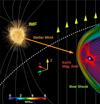 |
Fig. 1 3D view of a typical simulation setup. We show the density distribution (color scale), Earth magnetic field lines (red lines), and IMF (yellow lines). The yellow arrows indicate the orientation of the IMF (northward orientation). The dashed white line shows the beginning of the simulation domain (the star is not included in the model). |
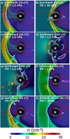 |
Fig. 2 Polar cut (XY plane) of the plasma density in simulations with (a) Sun–Earth IMF orientation |BIMF | = 10 nT Pd = 1.2 nPa, (b) Sun–Earth IMF orientation |BIMF| = 10 nT Pd = 30 nPa, (c) northward IMF orientation |BIMF| = 10 nT Pd = 1.2 nPa, (d) northward IMF orientation |BIMF| = 100 nT Pd = 1.2 nPa, (e) northward IMF orientation |BIMF| = 200 nT Pd = 1.2 nPa, (f) southward IMF orientation |BIMF| = 50 nT Pd = 3 nPa, (g) Earth–Sun IMF orientation |BIMF| = 50 nT Pd = 3 nPa, and (h) ecliptic ctr-cw IMF orientation |BIMF| = 50 nT Pd = 3 nPa. Earth magnetic field (red lines), SW stream functions (green lines), |B| = 10 nT isocontour of the magnetic field (pink lines), and vr = 0 isocontours (white lines). The bold cyan arrows show the regions in which the plasma is injected into the inner magnetosphere. |
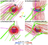 |
Fig. 3 3D view of the Earth magnetosphere topology if |B|IMF = 250 nT for (a) a Sun–Earth, (b) southward, (c) northward, and (d) ecliptic ctr-clockwise IMF orientations. We show the Earth magnetic field (red lines), SW stream functions (green lines), and isocontours of the plasma density for 6–9 cm−3, indicating the location of the BS (pink lines). The cyan isocontours indicate the reconnection regions (|B| = 60 nT). |
 |
Fig. 4 (a) Polar cut (XY plane) of the plasma temperature and (b) 3D view of the Earth magnetosphere adding the plasma temperature isocountour T = 26 keV (orange surface, temperature local maxima at R = 3 RE planet DS) and a polar/equatorial (XY∕XZ plane) cut of the plasma density for a simulation without an IMF and Pd = 1.2 nPa. The red lines indicate the Earth magnetic field lines. |
3.1 Parametric study of the magnetopause standoff distance
The magnetopause standoff distance Rsd can be calculated as the location where the dynamic pressure of the SW (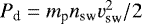 ), the thermal pressure of the SW (
 ), and the magnetic pressure of the IMF (
 are balanced by the magnetic pressure of the Earth magnetosphere of a dipolar magnetic field (
 ) and the thermal pressure of the magnetosphere (
 ). This results in the expression
 (5)
(5)
![\begin{equation*}\frac{R_{\textrm{sd}}}{R_{\textrm{E}}} = \left[\frac{\alpha \mu_{0} M_{\textrm{E}}^{2}}{4 \pi^2 \left(m_{\textrm{p}} n_{\textrm{sw}} v_{\textrm{sw}}^{2} + \frac{B_{\textrm{sw}}^{2}}{\mu_{0}} + \frac{2 m_{\textrm{p}} n_{\textrm{sw}} c_{\textrm{sw}}^{2}}{\gamma} - m_{\textrm{p}} n_{\textrm{BS}} v_{\textrm{th,MSP}}^{2} \right)} \right]^{(1/6)}\!\!\!\!,\end{equation*}](/articles/aa/full_html/2022/03/aa41181-21/aa41181-21-eq15.png) (6)
(6)
with ME the Earth dipole magnetic field moment, r = Rsd∕RE, and α the dipole compression coefficient (α ≈ 2; Gombosi 1994). This expression is an approximation, and it does not consider the effect of the reconnection of the Earth magnetic field with the IMF, that is to say, the approximation assumes a compressed dipolar magnetic field, ignoring the orientation of the IMF. Consequently, the theoretical standoff distance is only valid if |BIMF| is small, thus Rsd∕RE should be calculated using simulations for extreme space weather conditions. In the following, the location of the magnetopause is defined as the last close magnetic field line on the Earth DS at 0° longitude in the ecliptic plane. Figure 5 shows the pressure balance in simulations without IMF and low Pd, large |BIMF| and low Pd, as well as large |BIMF| and high Pd.
The simulation without IMF and Pd = 1.2 nPa shows a balance of the dynamic pressure of the SW and the combined effect of the magnetosphere magnetic and thermal pressure; see panels a to d of Fig. 5. The effect of the magnetosphere thermal pressure on the pressure balance for space weather conditions with low |BIMF| and Pd, leading to Pth,MSP∕Pmag,E ≈ 1.0 is strong. Figure 5, panels c and d, show two local maxima of Pth inside the BS and nearby the upper ionosphere. The Pth local maxima nearby the upper ionosphere are linked to the plasma belt (see Fig. 4), whose role on the pressure balance is negligible because the magnetic pressure generated by the Earth magnetic field in this plasma region is dominant, at least one order of magnitude higher. For a northward IMF with |BIMF| = 100 nT and Pd = 1.2 nPa, the leading terms in the pressure balance are the magnetic pressure of the IMF (Pd is 3.5 times lower) and the magnetosphere magnetic pressure (the magnetosphere thermal pressure is 4 times lower); see panels e to h. Consequently, the IMF orientation is particularly important for space weather conditions with a high IMF intensity but low SW dynamic pressure. On the other hand, the simulation for a northward IMF with |BIMF| = 50 nT and Pd = 60 nPa indicates a balance of the magnetic pressure of the magnetosphere (the magnetosphere thermal pressure is 4–5 times lower) and the combined effect of the SW dynamic pressure and the IMF magnetic pressure; see panels i to l. In other words, the leading terms of the pressure balance during extreme space weather conditions are the dynamic pressure of the SW, the IMF magnetic pressure, and the magnetosphere magnetic pressure.
We now study the effect of the IMF intensity and orientation on the magnetopause standoff distance. For this purpose, we fixed the SW parameters to Tsw = 1.8 × 10⁵ K and Pd = 1.2 nPa. First, we must clarify that the configurations we analyzed are idealizations, that is to say, an IMF that is purely oriented in one direction is rarely observed, particularly if the IMF intensity is high. This subtlety especially applies to the radial IMF configurations because small deviations in the ecliptic component break the East-West symmetry on the model, leading to a substantial variation in the Earth magnetosphere topology. Nevertheless, all the possible configurations were analyzed for the completeness of the study, independent of the rarity of the space weather condition. Figure 6 shows the location of the magnetopause in the ecliptic plane for different IMF orientations and intensities.
Two different trends are observed in Fig. 6 for Rsd ∕RE regarding the Ma value of the simulation. If Ma < 1, simulations with |BIMF|≤ 60 nT, the pressurebalance is dominated by the magnetic pressure of the IMF and the Earth magnetic field because the BS is not formed, thus the thermal pressure of the plasma inside the BS does not participate in the balance; see Fig. 2 panels d and e as well as Fig. 5 panels d to f. On the other hand, if Ma > 1, the thermal pressure of the plasma inside the BS participates in the balance, particularly in the simulations with low |BIMF| values; see Fig. 2 panels a and c as well as Fig. 5 panels a to d (Pth,MSP∕Pmag,E ≈ 0.4–1.0). The general trend in the simulations with Ma < 1 indicates a decrease in Rsd∕RE as the IMF intensity increases for all the IMF orientations. In contrast, Ma > 1 simulations for the Sun–Earth and Earth–Sun IMF orientations show an increase or a constant Rsd ∕RE, respectively. This exception is explained by the northward (southward) bending of the magnetosphere at the planet DS if the IMF is Earth–Sun (Sun–Earth), see Fig. 2 panel g, as well as the magnetosphere thermal pressure. The IMF orientation that leads to the lowest Rsd∕RE as |BIMF| increases is the Southward orientation, while the northward IMF orientation leads to the highest Rsd ∕RE. The data for each IMF orientation and Ma trend were fit to the expression  , indicated by solid lines for the simulations with Ma > 1 and by the dashed line for the Ma < 1 simulations in Fig. 6. Table 2 shows the fitting parameters of the regressions in the simulations with Ma < 1 and Ma > 1 for different IMF orientations.
The fit exponent of the simulations with Ma < 1 for northward, southward, and ecliptic IMF orientations are close to the theoretical α =−0.33 value from Eq. (6), neglecting the effect of the SW thermal and dynamic pressure as well as the magnetosphere thermal pressure. The excursion from the theoretical value is a consequence of the IMF orientation, that is to say, it is due to the deviation from the dipolar magnetic field assumption. The largest deviation is observed for the southward IMF orientation because the southward IMF leads to the strongest erosion of the Earth magnetic field on the DS and the largest decrease in magnetopause standoff distance. The exponents are negative because the magnetic pressure of the IMF is opposed to that of the magnetic pressure of the Earth magnetic field. On the other hand, the fit exponents for the Earth–Sun and Sun–Earth IMF orientations are more than twice higher than the theoretical value. The large deviation is explained by the formation of two Alfvén wings at the Earth’s DS and NS (Chane et al. 2012, 2015). Figure 7, panel a, shows the Alfvén wings that formed in the simulation with Earth–Sun IMF |BIMF| = 250 nT and Pd = 1.2 nPa. The Alfvén wings show the characteristic bending of the Earth magnetic field near the planet surface, the low-velocity plasma inside the wings, and a high-velocity plasma linked to the reconnection regions between the IMF and the Earth magnetic field. The IMF and Earth magnetic field magnetic pressure, see Fig. 7b, illustrates the role of the reconnection regions in the pressure balance and explains the large deviation of the fit exponents from the theoretical value. It must be pointed out that the Alfvén wings are observed during very special space weather conditions with extremely low SW densities, that is to say, the simulations performed do not represent the usual conditions for the formation of the Alfvén wings for the case of the Earth. Nevertheless, the study provides a generalization of the space weather conditions for the formation of the Alfvén wings in exoplanets with an Earth-like magnetosphere. The fit exponents of the simulations with Ma > 1 for northward, southward, and ecliptic IMF orientations are smaller than the theoretical value because the effect of the SW dynamic pressure and magnetosphere thermal pressure cannot be neglected. If |BIMF| increases, the magnetosphere thermal pressure decreases because the BS plasma is depleted faster: the reconnection regions are located closer to the Earth surface. Consequently, the pressure balance of the simulations with |BIMF|≥ 20 nT are dominated by the SW dynamic pressure and the combined effect of the magnetosphere thermal pressure and the Earth magnetic field pressure. Likewise, if |BIMF| > 20 nT, the combination of the SW dynamic pressure and the IMF magnetic pressure is mainly balanced by the Earth magnetic field pressure. The Earth–Sun and Sun–Earth IMF orientations show a weak dependence on |BIMF|, which is a consequence of the magnetosphere bending induced by the IMF in conjunction with the thermal pressure of the magnetosphere, which is almost unchanged as |B|IMF increases because the BS plasma depletion is rather weak due to the location of the reconnection region above 12 RE. This results in a magnetopause standoff distance that is nearly constant. The ecliptic clockwise and counterclockwise orientations lead to the same result.
We also considered the SW effect on the magnetosphere topology. To this end, IMF parameters were kept fixed (Sun–Earth IMF orientation with |B| = 10 nT). The IMF intensity in the simulations is small, minimizing the IMF effect on the magnetosphere topology. Figure 8 shows Rsd ∕RE for different SW densities (fixed Tsw = 1.8 × 10⁵ K and |v| = 350 km s−1, panel a), SW velocities (fixed Tsw = 1.8 × 10⁵ K and n = 12 cm−3, panel b), and corresponding dynamic pressures (panel c).
Rsd∕RE decreases asthe SW density or velocity increases, that is to say, a higher dynamic pressure leads to a stronger compression of the BS. Even if the dynamic pressure increases up to 160 nPa, extreme space weather conditions are comparable to a super-ICME, Rsd∕RE > 4.5. Consequently, the direct deposition of the SW toward the Earth surface requires a large distortion of the magnetosphere by the IMF in addition to the BS compression caused by the SW dynamic pressure. Again, the data were fit to the functions Rsd ∕RE = Anα, Rsd ∕RE = A|v|α, and  . In addition, three different data sets were used in the regression, the full range of values for the SW density and velocity (dashed black line), Pd < 10 nPa cases with n ≤60 cm3 and |v| ≤ 600 km s−1 (red solid line), and Pd > 10 nPa cases with n >60 cm3 and |v| > 600 km s−1 (solid blue line). No plateau is observed in the figures because the minimum dynamic pressure of the simulations is high enough to induce a relatively intense deformation of the magnetosphere. Table 3 shows the fitting result.
From Eq. (6), we deduce that the theoretical α exponent is − 0.17 for the SW density and − 0.33 for the SW velocity, assuming a negligible effect of the IMF magnetic pressure, SW thermal pressure, and magnetosphere thermal pressure in the pressure balance. The fit exponents are close to the theoretical exponents when the SW dynamic pressure is high enough (Pd≥ 10 nPa) to induce a significant compression of the magnetosphere (Rsd∕RE < 7), thus the pressure balance is dominated by the SW dynamic pressure and the magnetic pressure of the Earth magnetosphere; see the solid blue line in Fig. 8 panels a, b, and c. On the other hand, the regression exponents are 25% higher in the simulations with Pd < 10 nPa; see the solidred lines in panels a, b, and c. The deviation is caused by the effect of the magnetosphere thermal pressure on the pressure balance. The ratio of the magnetosphere thermal pressure and the SW dynamic pressure increases from 0.2 to 0.5 when the SW density decreases from 60 to 6 cm−3 and from 0.4 to 0.8 when the SW velocity decreases from 600 to 100 km s−1. Consequently, the magnetosphere thermal pressure must be included in the pressure balance to correctly calculate the magnetopause standoff distance when the SW dynamic pressure is low. The simulations without an IMF (pink stars) and the data fit (solid pink line) indicate the small effect of the Sun–Earth IMF with |B|IMF = 10 nT on the pressure balance and the Earth magnetic field topology. The regression extrapolation indicates a critical Pd ≈ 3.5 × 10⁵ nPa for the direct deposition of the SW toward the Earth surface, two orders of magnitude larger than the Pd values during a super-ICME for the case of the Earth. Consequently, the direct precipitation of the SW for a relatively weak |B|IMF is extremely unlikely.
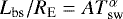
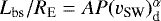
After the effect of the SW on the magnetopause standoff distance was assessed, we studied the effect of the plasma temperature and dynamic pressure on the thickness of the BS (Lbs∕RE), with Lbs the distance between the BS nose and the magnetopause standoff distance at the ecliptic plane on the DS 0° longitude. An increase in SW temperature leads to an increase in sound speed and thickness of the BS. On the other hand, a higher dynamic pressure leads to a compression of the BS. Figure 9 shows the Lbs∕RE values that were calculated in simulations performed for a range of the SW temperatures (fixed Pd ≈ 2 nPa, panel a) and the Pd values (fixed Tsw = 1.8 × 10⁵ K, panel b). In addition, the data were fit to the functions  and
and  .
.
The simulations indicate an increase in BS width of ≈ 0.4 RE when the SW temperature increases from 5 × 10⁴ to 2 × 10⁵ K (panel a). On the other hand, the BS width decreases ≈2.8 RE when Pd raises from 0.2 to 160 nPa (panel b). That is to say, the BS compression caused by the SW Pd is around 6–7 times higher than the BS expansion due to the SW temperature. Moreover, the BS compression is lower in the simulations with fixed SW velocity because the plasma temperature and sound speed inside the BS are higher as well as Pth. In addition, the simulations with Pd < 4 nPa show a weaker dependence of the BS width on Pd (compare the regression parameters of the simulations with Pd > 4 nPa and Pd < 4 nPa) because the magnetosphere thermal pressure is comparable to Pd. By contrast, as the simulation Pd increases and the role of the magnetosphere thermal pressure is less important in the pressure balance, the dependence of the BS width on Pd increases. The range of SW temperature and Pd values we highlighted includes the typical SW parameters during regular and extreme space weather conditions (Cliver et al. 1990; Mays et al. 2015).
In summary, the magnetopause standoff distance we calculated in the simulations reveals the key role of the IMF and SW in the distortion of the Earth magnetosphere for regular and extreme space weather conditions. The data regressions show clear differences in the pressure balance for super-Alfvénic and sub-Alfvénic configurations, as well as the important role of the magnetosphere thermal pressure in the determination of the magnetopause standoff distance when the SW dynamic pressure and IMF magnetic pressure are low. The range of magnetopause standoff distance we calculated iscomparable to the results obtained by other authors (Song et al. 1999; Kabin et al. 2004; Lavraud & Borovsky 2008; Ridley et al. 2010; Meng et al. 2012; Wang et al. 2015). The contribution of our study entails a larger sample of space weather configurations through the extended parametric studies we performed, as well as through the detailed analysis of the topological deformation trends that are linked to the SW and IMF properties.
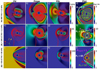 |
Fig. 5 Polar cut (XY plane) of the pressure balance. Simulation without IMF and Pd = 1.2 nPa, isocontour of(a) Pd, (b) Pmag and (c) Pth. Simulation with northward |BIMF| = 100 nT and Pd= 1.2 nPa, isocontour of(e) Pd, (f) Pmag, and (g) Pth. Simulation with northward |BIMF| = 50 nT and Pd= 60 nPa, isocontour of(i) Pd, (j) Pmag, and (k) Pth. Panels d, h, and l show the total pressure (Ptot = Pd + Pmag + Pmag,sw + Pth) normalized to the SW dynamic pressure (isocontour) as well as the isolines of Pd (white line), Pth (green line), Pmag (red line), and Pmag,sw (pink line), including the respective isoline values (colored characters). |
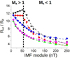 |
Fig. 6 Magnetopause standoff distance with respect to |B|IMF when the IMF is oriented in the Sun–Earth direction (black star), Earth–Sun (red circle), northward (blue diamond), southward (green triangle), and ecliptic ctr-clockwise direction (pink hexagon). The solid (dashed) lines indicate for each IMF orientation the data fit to the expression
|

Fit parameters of the regression  for different IMF orientations (first column) in simulations with Ma < 1 (second and third columns) and Ma > 1 (fourth and fifth columns).
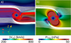 |
Fig. 7 Polar cut (XY plane) of the (a) plasma velocity module (color scale) and (b) magnetic pressure. The red lines indicate the magnetic field lines connected to the Earth surface, and the white lines show the unreconnected IMF lines. |
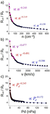 |
Fig. 8 Magnetopause standoff distance with respect to (a) the SW density (fixed v = 350 km s−1), (b) SW velocities (fixed 12⋅ cm−3), and (c) dynamic pressure. Sun–Earth IMF orientation with |B| = 10 nT. The pink stars indicate the magnetopause standoff distance if |B| = 0 nT. The dashed lines indicate the data fit to the expression Rsd∕RE = Anα, Rsd ∕RE = A|v|α, and |

Fit parameters of the regressions Rsd∕RE = Anα (first row), Rsd∕RE = A|v|α (second row), and  (third row) for the simulations with low (second and third columns) and high (fourth and fifth columns) Pd.
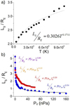 |
Fig. 9 BS width for (a) different SW temperatures (fixed Pd = 1.2 nPa) and (b) different Pd values (fixed Tsw = 1.8 × 10⁵ K) when the SW density increases (fixed the SW velocity to 350 km s−1, red dots) or the SW velocities increases (fixed the SW density to 12 cm−3, blue dots). Sun–Earth IMF orientation with |B| = 10 nT. The dashed lines indicate the data fit to the expression |


 |
Fig. 10 Location of the reconnection regions in the XY plane when |BIMF| increases from 10 to 250 nT for Earth–Sun and Sun–Earth IMF orientations. Pd = 1.2 nPa and Tsw = 1.8 × 10⁵ K. The color of the symbols indicates the |BIMF| value. The stars indicate the reconnection region for the Sun–Earth IMF orientation. The circles indicate the reconnection region for the Earth–Sun IMF orientation. |
3.2 Reconnection region tracking for different IMF orientations and intensities
This section is dedicated to tracking the location of the reconnection regions for different IMF orientation and intensities. Figure 10 indicates the location of the reconnection regions in the XY plane for Sun–Earth and Earth–Sun IMF orientations as |BIMF| increases from 10 to 250 nT. Likewise, Fig. 11 shows the same study for northward and southward IMF orientations. The reconnection in the simulations is identified as the region in which the magnetic field intensity goes to zero.
The reconnection region for the Sun–Earth IMF orientation on the DS moves toward the South pole as |BIMF| increases, showing a large northward displacement, but this is smaller in the Earth-ward direction. On the other hand, the reconnection on the NS moves toward the North pole, and the larger displacement is found in the sunward direction with respect to the southward displacement. Regarding the Earth–Sun IMF orientation, the reconnection on the DS moves southward toward the North pole, although the reconnection on the NS moves toward the South pole. The differences between the Sun–Earth and Earth–Sun orientations are caused by the North-South bending of the Earth magnetosphere. The reconnection region on the NS is located outside the computational domain for the simulations with |BIMF| < 30 nT, thus these data were not included in the analysis.
The reconnection region in the simulations with a southward IMF orientation are located closer to the equatorial plane and the Earth surface as |BIMF| increases. On the DS, the reconnection displaces southward and earthward. Regarding the northward IMF orientation, the reconnections are located closer to the poles as |BIMF| increases. The reconnection region on the NS is outside the computational domain for the simulations with southward IMF and |BIMF| < 60 nT, and also for the simulations with northward IMF and |BIMF| < 40 nT. These regions were not considered.
Figure 12 shows the location of the reconnection region for an ecliptic ctr-clockwise IMF orientation as |BIMF| increases. The clockwise case is not included because the Earth magnetosphere shows a symmetric topology deformation with respect to the ecliptic IMF orientations. The analysis is more complex regarding the other IMF orientations because the reconnections are not located in the XY plane and should be tracked in 3D.
The reconnection regions move toward the planet surface as the |BIMF| increases, following the East/West tilt induced in the Earth magnetosphere. The reconnection region is outside the computational domain for the simulations with |BIMF| < 20 nT.
To summarize, the location of the reconnection regions is critical for understanding the effect of the IMF orientation and intensity on the topology of the Earth magnetosphere. The study reveals a large variation in this topology in the range of IMF intensities and orientations we analyzed. Consequently, the SW injection into the inner magnetosphere and the plasma flows toward the Earth surface are very different regarding the IMF configuration. Table 4 shows the percentage of the reconnection displacement for different IMF orientations (defined as 100 ⋅ Δrmax∕Δrmin with  ) between the simulations with |BIMF| = 250 nT and |BIMF|min (third and fifth columns). The third and fifth columns also indicate whether the reconnection regions are located on the DS, NS, at the North pole, South pole, and West or East of the magnetosphere. If the reconnection region is located outside the computational domain (because |BIMF| is small), the simulation is not included in the analysis and the configuration with the lowest |BIMF| with the reconnection region inside the computational domain is indicated in the table (second and fourth columns).
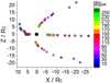 |
Fig. 11 Location of the reconnection regions in the XY plane when |BIMF| increases from 10 to 250 nT for northward and southward IMF orientations. Pd = 1.2 nPa and Tsw = 1.8 × 10⁵ K. The color contour indicates the |BIMF| value. The yellow (gray) star indicates the reconnection region on the DS (NS) for a southward IMF orientation. The yellow (gray) circle indicates the reconnection region near the North (South) pole for the northward IMF orientation. |
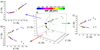 |
Fig. 12 Location of the reconnection region if |BIMF| increases from 10 to 250 nT for an ecliptic ctr-clockwise IMF orientation. Pd = 1.2 nPa and T = 1.8 × 10⁵ K. The color contour indicates the |BIMF| value. Panel a indicates the projection in the Y Z plane, (b) the projection in the XZ plane, and (c) the projection in the XY plane. Paneld shows the 3D view. |
IMF orientation (first column).
3.3 Open and closed field line boundary for different IMF orientations and intensities
The modification of the topology of the Earth magnetosphere by the IMF also modifies the ratio between open and closed magnetic field lines at the Earth surface. The Earth surface covered by open field lines is more vulnerable to extreme SW conditions because the plasma precipitates along the magnetic field lines toward the surface. If a large amount of SW is injected into the inner magnetosphere through the reconnection regions, the plasma flows on the planet surface, which is covered by open field lines, are higher. Consequently, it is important to study the modification that the IMF intensity and orientation cause on the latitude of the open and closed field line boundary (OCB). Figure 13 shows the open magnetic field lines at R∕RE = 2.05 for different IMF intensities and orientations (fixed Pd = 1.2 nPa and Tsw = 1.8 × 10⁵ K). The OCB lines are identified by an iterative method that calculates the last close magnetic field line connecting the inner boundary of the computational domain and concentric spheres with radius between Rsd ∕RE and (Rsd + RE)∕RE. The magnetotail is fully located inside the simulation domain in the configurations we analyzed; see the Appendix C for further discussion.
The increase in |BIMF| for a Sun–Earth IMF orientation (panel a) causes a decrease in OCB latitude on the DS, which is particularly large in the North Hemisphere. This result is consistent with the southward bending of the Earth magnetosphere, promoting a stronger erosion of the Earth magnetic field by the IMF in the North Hemisphere. The east-west tilt of the magnetosphere caused by the IMF orientations in the ecliptic plane (panel b) is also observed in the open field line distribution, leading to a large longitudinal and latitudinal OCB dependence. Regarding the Sun–Earth and Earth–Sun IMF orientations (panels c and d), the OCB is asymmetric with respect to the DS and NS. On the other hand, the displacement of the reconnection regions toward the Earth magnetic axis (equatorial plane) for a northward (southward) IMF orientation leads to a displacement of the OCB towards a higher (lower) latitude (panels e and f). The southward IMF orientation leads to the lowest OCB latitude on the DS and NS for both hemispheres.
The latitude of the OCB at the Earth surface was calculated by mapping the magnetic field lines obtained in the simulations with the magnetic field of a dipole without the distortion of the SW and IMF. The magnetic field line mapping is described in the Appendix B, where we show that below 2RE, the unperturbed and perturbed dipoles agree well, thus the OCB line latitude at the Earth surface can be extrapolated with reasonable confidence. Figure 14 indicates the OCB latitude with respect to the IMF orientation and |BIMF| calculated on the Earth DS (0° longitude) and NS (180° longitude) in the Northand South Hemispheres. In addition, the OCB latitude is compared with the latitude of the auroral oval associated with different Kp indices. The Kp index indicates the global geomagnetic activity. It takes values from 0 for the case of weak geomagnetic activity to 9 if there is extreme geomagnetic activity (Menvielle & Berthelier 1991; Thomsen 2004).
The OCB latitude on the North Hemisphere DS (panel a) decreases from 70° to 58° as |BIMF| increases for the Sun–Earth IMF orientation. Regarding the Earth–Sun IMF orientation, the range of OCB latitudes is slightly smaller, between 68 − 58°, due to the northward bending of the magnetosphere on the DS, leading to slight differences with respect to the Sun–Earth IMF in the North Hemisphere, but causing larger differences in the South Hemisphere (panel c). On the other hand, the northward IMF orientation leads to an increase in OCB latitude in the North Hemisphere up to 80° if |BIMF| = 100 nT, which decreases to 76° if |BIMF| = 250 nT due to the combined effect of the magnetosphere compression and the tilt. On the other hand, the OCB latitude in the South Hemisphere increases when |BIMF| reaches 88° for |BIMF| = 250 nT simulation. The trend of the OCB latitude regarding |BIMF| is inverted between hemispheres on the planet NS (see Fig. 10), again due to the effect of the magnetic field tilt. For the southward IMF orientation, the OCB latitude decreases as |BIMF| increases, between 63–53° in the North Hemisphere and 63–51° in the South Hemisphere if the simulations with |BIMF| = 10 and 250 nT are compared due to the Earth magnetic field erosion at the equatorial region. For the ecliptic ctr-clockwise orientation, the OCB latitude slightly decreases as |BIMF| increases, from 65° to 61° when |BIMF| increases from 10 to 250 nT, because the west-east asymmetry induced in the magnetosphere has a lesser effect on the OCB latitude. The latitude of the auroral oval for different Kp index is included in the panels and compared with the OCB latitude at the Earth DS and NS, providing an approximation of the Kp index in the simulations. The largest variation in OCB line with respect to the Kp index as |BIMF| enhances is observed for the Earth–Sun and southward IMF orientations. Consequently, Earth–Sun and southward IMF orientations can lead to strong geomagnetic activities. This result is consistent with previous studies by Schatten & Wilcox (1967); Boroyev et al. (2020). The Sun–Earth, northward, and ecliptic IMF orientations lead to Kp ≤ 4 if |BIMF| = 250 nT, thus the geomagnetic activity that is caused is relatively quiet. The latitudinal resolution of the model is 4°, thus the uncertainly on the Kp index prediction is ± 2, which is enough to distinguish between quiet (Kp < 3), moderate (3 ≤ Kp ≤ 6), and strong (Kp > 6) auroral activity.
In summary, the OCB latitude, and so the exposition of the Earth surface to the plasma flows from the magnetosheath, shows a clear dependence on the space weather conditions, leading to a large decrease in OCB latitude, in particular for an intense southward oriented IMF. For example, Fig. 15 shows the OCB line for different IMF orientations with |BIMF| = 250 nT, indicating that the South of Canada and the North of England are exposed if the IMF orientation is southward, thus the electric grids of these countries are in danger. Similar trends were obtained by other authors with respect to the IMF orientation and intensity (Lopez et al. 1999; Kabin et al. 2004; Wild et al. 2004; Wang et al. 2016; Burrell et al. 2020). We extended and refined these results here through the large sample of parametric studies we performed, including a forecast of the Kp index variation with respect to the IMF module and orientation.
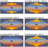 |
Fig. 13 Sinusoidal (Sanson-Flamsteed) projection of the open and closed magnetic field line boundary at R∕RE = 2.05 for (a) |BIMF| = 0 nT, (b) ecliptic ctr-clockwise |BIMF| = 250 nT, (c) Sun–Earth |BIMF| = 250 nT, (d) Earth–Sun |BIMF| = 250 nT, (e) northward |BIMF| = 250 nT, and (f) southward |BIMF| = 250 nT. Fixed Pd = 1.2 nPa and Tsw = 1.8 × 10⁵ K. The yellow (orange) dots indicate the open magnetic field lines at the Earth DS (NS). |
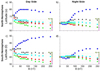 |
Fig. 14 OCB latitude with respect to the IMF orientation and |BIMF| calculated inthe North Hemisphere (a) DS (0° longitude) and (b) NS (180° longitude), South Hemisphere (c) DS and (d) NS. Fixed Pd = 1.2 nPa and Tsw = 1.8 × 10⁵ K. The dashed horizontal lines indicate the Kp index. The yellow star indicates the OCB latitude if |BIMF| = 0. IMF direction: Sun–Earth (black star), Earth–Sun (red circle), northward (blue diamond), southward (green triangle), and ecliptic ctr-clockwise (cyan pentagon). |
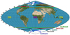 |
Fig. 15 Schematic view of the OCB line for Sun–Earth (black line), Earth–Sun (red line), northward (blue line), southward (green line), and ecliptic ctr-clockwise (cyan lines) with |BIMF | = 250 nT. The parameters Pd = 1.2 nT and Tsw = 1.8 × 10⁵ K are fixed. The location of the DS and NS with respect to the continents is irrelevant. |
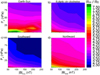 |
Fig. 16 Isocontour of the magnetopause standoff distance for different Pd and |BIMF| values when the IMF is oriented (a) Earth Sun, (b) ecliptic ctr-clockwise, (c) southward, and (d) northward. The parameter T = 1.8 × 10⁵ K is fixed. |
3.4 Combined effect of the dynamic pressure and IMF orientation and intensity on the topology of the Earth magnetic field
A complete parametric study of the topology of the Earth magnetosphere with respect to space weather conditions requires the combined effect of the SW dynamic pressure and the IMF module and orientation. With this aim, Fig. 16 indicates the magnetosphere standoff distance with respect to the IMF orientation and module (for |BIMF| = 50, 100, 150, 200 and 250 nT) and the SW dynamic pressure (Pd = 1.2, 1.5, 3, 4.5, 6, 15, 30, 45, 60, 80, and 100 nPa). The range of parameters includes regular and extreme space weather conditions (ICME). Ecliptic clockwise and counterclockwise IMF orientations lead to the same results. We therefore only analyzed the counterclockwise case. The Sun–Earth orientation is not included because in spite of the magnetic field tilt, there is an North-South symmetry with respect of the Earth–Sun orientation so that the simulations results are similar.
The IMF orientation that leads to the smallest magnetopause standof distance with respect to |BIMF| and Pd is the southward orientation. The simulations indicate that for Pd and |B|IMF. values consistent with extreme space conditions such as an ICMEs impacting the Earth (|B|IMF ≈ 100 nT and Pd ≈ 30 nPa), there is no direct precipitation of the SW toward the Earth surface. The smallest Rsd ∕RE = 2.92 is obtained for the southward IMF orientation. In addition, super-CMEs with |B|IMF = 250 nT and Pd = 100 nPa and an IMF oriented in the southward direction just lead to a Rsd∕RE slightly below 2.5, which is higher than 2.8 for the remaining IMF orientations. The balance between the dynamic pressure and IMF intensity is particularly complex for the Earth–Sun IMF orientation for simulations with Pd < 30 nPa, leading to an increase in Rsd∕RE as |B|IMF increases. This is caused by the North-South deformation that is induced at the DS and NS of the magnetosphere. On the other hand, simulations with Pd > 30 nPa, Rsd ∕RE show a weak dependence on |B|IMF because the compression of the BS is partially counterbalanced by the North-South asymmetry induced in the magnetosphere.
Next, Rsd∕RE data were fit with respectto Pd and |B|IMF by the surface function  . The regression results are indicated in Table 5 and Fig. 17. The regression analysis for the southward IMF orientation only includes Pd < 60 nPa values, thus the simulations with Rsd∕RE < 2.5 are not included in the study.
The expected exponents from the Eq. (6) are α =−0.33 and β =−0.17, although the regressions show clear deviations mainly caused by the Earth magnetic field reconnection with the IMF, particularly in the simulations with large |B|IMF, as well as the pressure generated by the particles inside the BS in the simulations with low Pd. The largest deviation of the α exponent is observed for the ecliptic and northward IMF orientation because there is a strong West-East tilt and poleward stretching induced in the magnetosphere that is further promoted in simulations with large Pd. In the southward IMF orientation, the α exponent is smaller than the theoretical value because of the erosion induced in the Earth magnetic field at the equatorial region. On the other hand, the Earth–Sun IMF orientation shows an α exponent that is closer to the theoretical value because the induced northward bending of the magnetosphere is weaker as the simulation Pd increases. The β exponent of the regressions agrees reasonably well with the theoretical exponent, although the deviation is significant regarding the ecliptic and northward IMF orientation cases for the reasons already mentioned.
In conclusion, the SW dynamic pressure, IMF intensity, and orientation are the main parameters required to study the response of the Earth magnetosphere to space weather conditions. Thus, the trends of the topological deformations identified by the parametric study can be generalized, providing a new tool for analyzing the consequences of the magnetosphere distortion. This is the topic of the following section.
Fit parameters of the regression  and standarderrors.
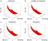 |
Fig. 17 Plot of the surface function |

4 Analysis applications
This section shows several applications of the study conclusions. Particularly, the direct exposition of satellites in different orbits to the SW for different space weather conditions, the Earth habitability along the solar main sequence, and an ICME classification with respect to the |B|IMF, Pd, and Dst parameters.
4.1 Forecast of space weather conditions for the SW precipitation toward the Earth surface
Figure 18 shows the critical |B|IMF required for the direct precipitation of the SW toward the Earth surface with respect to Pd and the IMF orientation. The SW precipitates directly toward the Earth surface if the magnetopause standoff distance of the simulation is the same as the Earth radius. Thus, the critical |B|IMF is calculated from the regression parameters taking Rsd∕RE = 1, thus ![$ \textrm{ln} (|B|_{\textrm{IMF,c}}) = ln [(A P^{\beta})^{-1}] / \alpha$](/articles/aa/full_html/2022/03/aa41181-21/aa41181-21-eq22.png) .
.
The direct precipitation of the SW requires the combination of extreme Pd and |B|IMF values well above the space weather conditions at the Earth even during super-ICME. For example, a southward IMF orientation with |B|IMF = 1000 nT requires Pd ≥ 355 nPa, while an Earth–Sun IMF orientation requires Pd ≥ 3660 nPa, which is 5–4 times larger than a super-ICME. Ecliptic and northward IMF orientations require even larger |B|IMF and Pd combinations for the direct precipitation of the SW.
4.2 Space weather conditions for the direct exposition of satellites to the solar wind
The direct exposition to the SW can inflict failure of the satellite electronics by radiation damage and charging. The Earth magnetic field protects the spacecraft, although the distortion of the magnetosphere driven by space weather conditions can lead to excursions outside the inner magnetosphere along the satellite orbit, particular at the Earth DS, where the magnetosphere is compressed by the SW and eroded by the IMF. Consequently, it is important to analyze the space weather conditions that can lead to the direct exposition of satellites at different orbits to the SW. The satellite orbits around the Earth are classified into low orbits (below 2000 km), medium orbits (between 2000–35 786 km), geosynchronous and geostationary orbits (at 35 786 km), and high orbits (above 35 786 km). Figure 19 indicatesthe critical Pd for different IMF intensities and orientations required to reduce the magnetopause standoff distance below the geostationary orbit Rgo = R∕RE ≈ 6.6 (panel a) and medium orbits at Rmo = R∕RE = 4.125 (20 000 km, panel b) and 2.5625 (10 000 km, panel c).
For the satellites on a geostationary orbit (panel a), during regular space weather conditions with Pd ≈ 1 nPa there is a transit outside the inner magnetosphere at the Earth DS if the IMF orientation is Earth–Sun and |B|IMF > 150 nT, decreasing to 130 nT for a northward IMF. The |B|IMF decreases to 50–60 nT if the IMF is southward or ecliptic ctr-cw. That is to say, southward and ecliptic IMF orientations are adverse for geostationary satellites because Rsd∕RE decreases below Rgo due to the erosion of the magnetic field at the DS and the East–West asymmetry driven in the magnetosphere. Likewise, if the space weather conditions lead to an enhancement of Pd, the geostationary satellites are exposed for southward IMF with |B|IMF = 10 nT and Pd ≈ 14 nPa, as well as ecliptic IMFwith |B|IMF = 10 nT and Pd ≈ 26 nPa.
On Earth medium orbits, a satellite at 20 000 km is exposed during regular space weather conditions with Pd ≈ 1 nPa if |B|IMF > 260 nT for a southward IMF, |B|IMF > 360 nT for an ecliptic IMF, |B|IMF > 600 nT for an Earth–Sun IMF and |B|IMF > 1450 nT for a northward IMF. Consequently, satellites on orbits of 20 000 km and lower are protected by the magnetosphere during regular space weather conditions because the critical |B|IMF is too large. On the other hand, extreme space weather conditions lead to exposed satellites at 20 000 km for southward IMF with |B|IMF = 40 nT and Pd ≈ 20 nPa, ecliptic IMF with |B|IMF = 40 nT, and Pd ≈ 55 nPa, Earth–Sun IMF with |B|IMF = 100 nT and Pd ≈ 60 nPa, as well as northward IMF with |B|IMF = 100 nT and Pd ≈ 70 nPa. In addition, satellites on an orbit of 10 000 km are only exposed if the IMF is southward, |B|IMF = 100 nT and Pd ≈ 70 nPa.
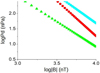 |
Fig. 18 Critical |B|IMF required for the direct precipitation of the SW toward the Earth surface with respect to Pd and the IMForientation. Fixed Tsw = 1.8 × 10⁵ K. IMF direction: Earth–Sun (red circle), southward (green triangle), and ecliptic ctr-clockwise (cyan pentagon). |
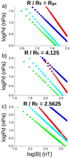 |
Fig. 19 Critical Pd to reducethe magnetopause standoff distance below (a) the geostationary orbit (b) medium orbit at Rmo =R∕RE = 4.125 and (c) medium orbit at 2.5625 for different IMF intensities and orientations. Fixed T = 1.8 × 10⁵ K. IMF direction: Earth–Sun (red circle), northward (blue diamond), southward (green triangle), and ecliptic ctr-clockwise (cyan pentagon). |
4.3 ICME classification
Most of the ICMEs that impact the Earth, around 1000 in each solar cycle, show an averaged plasma velocity lower than 500 km s−1 and IMF intensities below 15 nT. This leads to geomagnetic storms with Dst < −50 nT (Cane & Richardson 2003). Super-ICME events similar to the Carrington event are less frequent. They occur about once in each century (Riley et al. 2018), although the potential damage in space and ground technological resources is large (Baker et al. 2013; Eastwood et al. 2017, 2018). Other examples of super-ICME that did not impact the Earth were analyzed by Liu et al. (2014) using STEREO data, indicating plasma velocities about 2000 km s−1, a density of 100 cm−3 (Pd ≈ 330 nPa), and |B|IMF ≈ 100 nT (Dst = −600 to − 1100 nT). Space weather conditions during ICMEs can also be modeled using ENLIL (Odstrcil & Pizzo 1999; Odstrcil et al. 2002), the EUropean Heliospheric FORecasting Information Asset (EUHFORIA; Pomoell & Poedts 2018), and the Susanoo model (Shiota & Kataoka 2016), among others. Combining satellite data and modeling results, a classification of the ICMEs is proposed in Table 6 with respect to the SW dynamic pressure, IMF intensity, and Dst parameter.
When the results of our study are analyzed in the context of the proposed ICME classification, the direct precipitation of the SW toward the Earth surface is very unlikely, even for the case of super-ICMEs. The direct SW precipitation during a super-ICMEfor a southward IMF orientation requires extreme space weather condition values well above the expected range of the Pd and |B|IMF values, as was discussed in previous sections. Nevertheless, extreme space weather conditions inside the category of strong ICMEs already lead to magnetopause standoff distances of about Rsd ∕RE ≈ 2.5 if Pd = 60 nPa and |B|IMF = 100 nT for a southward IMF orientation, Rsd∕RE ≈ 3.8 for an Earth–Sun IMF orientation, Rsd∕RE ≈ 3.2 for an ecliptic IMF orientation, and Rsd∕RE ≈ 4.1 for a northward IMF orientation. Consequently, strong ICMEs are a threat to satellites on geostationary, high, and medium orbits. In particular the geostationary satellites are above the magnetopause for all the range of space weather condition inside the strong ICME category and IMF orientations. In addition, the medium-orbit satellites at 20 000 km are above the magnetopause if the IMF is southward for all the range of space weather condition inside the strong ICME category. It should be noted that medium-orbit satellites at 20 000 km are inside the inner magnetosphere if the IMF is northward during strong ICME space weather conditions. Medium-orbit satellites at 10 000 km are protected by the magnetosphere during strong ICME space weather conditions, although they are exposed to the direct impact of the SW during super-ICME space weather conditions in particular for the southward IMF orientation.
ICME classification with respect to the SW dynamic pressure, IMF intensity, and Dst parameter.
4.4 Earth habitability during the early-Sun main sequence
This section is dedicated to the analysis of the Earth habitability with respect to the space weather conditions during the solar evolution on the main sequence. Early stages of the solar evolution are linked to a faster rotation rate and higher magnetic activity (Emeriau-Viard & Brun 2017) because the solar rotation and magnetic activity decrease during the main sequence (Folsom et al. 2017; Fabbian et al. 2017). Consequently, the space weather conditions change (Réville et al. 2016; Carolan et al. 2019; Ahuir et al. 2020). When we consider the rotation tracks from Carolan et al. (2019) (Table 1), the average values of the SW radial velocity, density, and radial IMF intensity for different solar rotation rates are provided, thus the effect of the space weather conditions on the Earth magnetosphere during different stages of the solar evolution on the main sequence can be studied in the first approximation. The actual rotation rate of the Sun (ΩS) decreased from 10ΩS to 2ΩS between the first 300 to 1100 Myr of the solar evolution. The SW density approximately decreased from 1000 to 140 cm−3, the radial velocity from 1100 to 700 km s−1 (Pd drops from 980 to 57 nPa), and |B|IMF from 150 to 7 nT. Table 7 shows the averaged magnetopause standoff distance for a southward IMF during regular space weather condition with respect to ΩS based on the parametric study (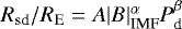 ). The uncertainty of Rsd∕RE is calculated as
  .
.
The analysis results indicate that the Earth magnetosphere avoids the direct precipitation of the SW during regular space weather condition if Ω =5–10ΩS, consistent with Carolan et al. (2019) analysis. Nevertheless, super-CMEs during the early main sequence of the Sun were probably more frequent, intense, and lasted longer (two or three days) (Sterenborg et al. 2011; Airapetian et al. 2015a,b), as the detection of superflares by Kepler mission for main-sequence G-K stars suggests (Shibayama et al. 2013). Figure 20 shows the range of parameters required for the direct precipitation of the SW during regular and CME space weather conditions on the early main sequence of the Sun (Ω = 5–10ΩS and <440 Myr). For simplicity, the space weather conditions consistent with CMEs on the solar early main sequence are in the range of 1 to 20 times the averaged Pd and |B|IMF values provided by Carolan et al. (2019). Only the data for southward IMF orientations are shown. They lead to the most restrictive space weather conditions.
The analysis shows a possible direct precipitation of the SW during early phases of the solar main sequence for CME-like space weather conditions, particularly if the solar rotation rate is 10ΩS. This indicates a wide range of parameters that lead to Rsd∕RE < 1.
In summary, the emerging life at the Earth surface was protected from the sterilizing effect of the SW during regular and CME-like space weather conditions 1100 Myr after the Sun entered the main sequence. On the other hand, during the first 440 Myr of the solar main sequence, CMEs and super-CMEs were a major hazard for Earth habitability, especially due to the high recurrence and prevalence of extreme space weather conditions. Our study results are comparable with the studies by See et al. (2014); Airapetian (2016).
Averaged magnetopause standoff distance for a southward IMF during regular space weather condition with respect to ΩS.
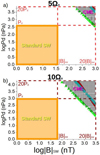 |
Fig. 20 Critical Pd and |B|IMF values for the direct precipitation of SW toward the Earth surface for a southward IMF if (a) 5ΩS and (b) 10ΩS. The dashed gray region indicates the space weather conditions that lead to the direct precipitation of the SW toward the Earth surface. The dashed orange region shows the regular space weather conditions. The parameter T = 1.8× 10⁵ K is fixed. |
4.5 Simulation of ICMEs impacting Earth between 1997 and 2020
A set of simulations was performed to reproduce the space weather conditions during the ICMEs that reached Earth between 1997 and 2020. The CMEs included in the analysis are a subsample of the CME Richardson list (Richardson & Cane 2020). We selected the most extreme events with respect to the Pd and |B|IMF values. They are listed in Appendix D. In the proposed ICME classification, all the events are common ICMEs, except for the space weather conditions on 16∕07∕2000 and 24∕11∕2001, which are close to the strong ICME category (Pd ≈ 30 nPa and |B|IMF ≈ 50 nT). Table 8 indicates the location of the nose of the BS, magnetopause standoff distance, and the lowest OCB latitude at the DS and NS in the North and South Hemispheres for the ICMEs we analyzed. In addition, the Kp index was calculated from the lowest latitude of OCB line in the North Hemisphere. The IMF and SW values we used as the simulation input represent the combination of SW dynamic pressure, IMF module, and southward IMF component that causes the strongest disturbance of the Earth magnetosphere during the ICME, but not necessarily the highest dynamic pressure, IMF module, and southward IMF component because these maxima may occur at different times. Figures D.1 and D.2 show the 24-h evolution of the IMF module and components, the velocity module and radial component, as well as the SW density and temperature for 15∕05∕1997 and 31∕03∕2001. The model resolution in the latitudinal direction is doubled, reducing the uncertainty of the OCB line from 4° to 2°, thus the uncertainty of the calculated Kp index is ± 1.
The ICMEs that led to the smallest magnetopause standoff distance impacted the Earth on 24∕11∕2001 and 29∕05∕2003 with Rsd ∕RE < 3.4. The lowest OCB latitudes in the North and South Hemispheres, <53°, were observed for the ICMEs on 31∕03∕2001b, 24∕11∕2001, 15∕05∕2005, and 24∕08∕2005, that is to say, the North of Canada, Alaska, North of Russia, and in the Nordic countries (except for continental Denmark) are exposed to plasma precipitation along the open magnetic fields. The calculated Kp index derived from the lowest OCB line latitude in the North Hemisphere is consistent with the measured Kp considering the ± 1 uncertainty, except for the 29∕05∕2003 ICME, for which the calculated Kp index is twounits smaller than the measured index. The aurora is generated by the electrons and ions precipitating toward the Earth surface, thus the plasma flows in the simulations must also be analyzed. Figure 21 indicates the plasma flows and velocity isocontours of the inflow regions at R∕RE = 2.75 for ICMEs on 31∕03∕2001b, 24∕11∕2001, 15∕05∕2005, and 24∕08∕2005 (ICMEs with the largest observed Kp = 8 index). In addition, Table 9 shows the latitude of the plasma flow extrapolated to the Earth surface in the North and South Hemispheres (inflow plasma velocity ≥ 50 km s−1).
The simulations indicate the formation of plasma streams connecting the magnetosheath and the Earth surface (see Fig. 21, blue and isolines). Regarding the IMF orientation, the inflow plasma regions on the Earth DS show an East-West asymmetry caused by the large IMF component on the ecliptic plane, for example, for the 24∕11∕2001 ICME, or a North–South asymmetry due to the IMF component on the Sun–Earth direction, for example, for the 24∕08∕2005 ICME. When the plasma flows are extrapolated to the Earth surface (v ≥ 50 km s−1, cyan line isoline), the plasma streams are deposited on the planet DS between the latitudes 50–74°. The simulation of the 24∕08∕2005 ICME shows the plasma deposition in the lowest latitude at the North Hemisphere DS 50–62°, although the simulation of the 21∕01∕2005 ICME indicates the widest plasma deposition region at the North Hemisphere DS 51–69°. Consequently, the plasma streams scatter from the OCB line and are deposited at the Earth surface from lower latitudes (between 2–3° below the OCB line latitude). If the Kp index is calculated including the scattering of the plasma streams, the Kp index for the simulations analyzed is 8, the same value as the measured Kp index. Regarding the plasma flows towards the Earth NS, the inflow maximum (v ≥ 200 km s−1, dark blue isoline) is observed between 54–56° latitude, consistent with the latitude of the aurora observations during extreme space weather conditions (Shaw 2019; Hayakawa et al. 2018; Mikhalev 2019). The plasma flows for the remaining ICME simulations is lower than that of the highlighted cases.
Figure 22 shows the OCB line calculated for the 27∕05∕2017 ICME simulations and the energy flux calculated by Ovation Prime simulations for 27∕05∕2017 t = 22 : 00 hours in the North and South Hemisphere. The Ovation Prime model is used to forecast the latitude and longitude of the visible aurora (Newell et al. 2010; Machol et al. 2012). Ovation prime data are provided by the integrated Space Weather Analysis system (iSWA; iSW 2020).
The latitude of the OCB line on the Earth NS is located between 58–64° in the North Hemisphere and 59–65° in the SouthHemisphere, similar to the Ovation prime forecast of the aurora location that indicates a local maxima of the energy flux between latitudes 58–65°. In addition, the Kp index derived from the OCB line is 5, which is the same value as the measured Kp index on 27∕05∕2017 at t = 22 : 00 h.
Figure 23 shows the satellites at geosynchronous, high, medium, and low orbits around the Earth with respect to the location of the BS nose and magnetopause standoff distance calculated from the ICME simulation results, in particular for the space weather conditions leading to the smallest magnetopause standoff distance that threatens the satellite integrity by direct exposition to the SW.
The space weather conditions for the 16∕07∕2000, 31∕03∕2001b, 24∕11∕2001, 29∕05∕2003, 21∕01∕2005 and 15∕05∕2005 ICMEs lead to RBS < Rgo, that is to say, the geosynchronous satellites directly face the SW during a fraction of the orbit on the Earth DS. Consequently, the integrity of geosynchronous satellites is in danger, especially because of the high SW density, up to 50 cm−3. On the other hand, the space weather conditions during the 03∕08∕2016 ICMEs led to Rsd > Rgo, thus the geosynchronous satellites are inside the Earth inner magnetosphere during the full orbit. The space weather conditions during the remaining ICMEs we analyzed show a RBS > Rgo > Rsd, thus the geosynchronous satellites are inside the Earth magnetosphere during the full orbit, although for a fraction of the orbit on the DS, the satellites cross the magnetosheath and enter the BS. Inside the BS, the SW particles slow down and accumulate, leading to a decrease in protection from the magnetosphere. The model developed by Dmitriev et al. (2016) predicted the magnetopause crossing of geosynchronous satellite during the 20∕11∕2003, 07∕11∕2004, 15∕05∕2005 and 24∕08∕2005 ICMEs, consistent with simulation results that indicate a magnetopause standoff distance below the geosynchronous satellite orbit: 4.29, 3.48, 3.88, and 3.52 RE, respectively. In addition, observations of magnetopause crossings by the geosynchronous satellite 1991 − 080, 1994 − 084 and LANL − 01A during 31∕03∕2001 ICME (Ober et al. 2002), by GOES 13 − 15 and MMS during 17∕03∕2001 ICME (Le et al. 2016), by THEMIS A and E during 27∕05∕2017 ICME (Pezzopane et al. 2019) are reported. They are also consistent with the simulation results, which predict a magnetopause standoff distance of 4.01, 5.30, and 5.33 RE, respectively. The satellites on medium orbits below 10 000 km are inside the magnetosphere throughout the full orbit for all the ICMEs we analyzed, although medium orbits on 20 000 km crossed the magnetosheath during the 22∕10∕1999, 31∕03∕2001, 24∕10∕2003, 07∕11∕2004, and 24∕08∕2005 ICMEs. Examples of the consequences of the severe space weather conditions during the 24∕10∕2003 ICME are the loss of the low-orbit satellite ADEOS/MIDORI 2 due to electrostatic discharge, the engine switch-off of the high-orbit satellite SMART-1 caused by the ionization effect of the SW, two weeks outage of the geostationary satellite DRTS/Kodama that wasalso caused by electrostatic discharge, as well as high bit error rates and magnetic torques that disabled GOES 9, 10, and 12 (Tamaoki et al. 2010; Cannon et al. 2013). The simulation of the 24∕10∕2003 ICME predicts a minor-moderate auroral activity, a significant East–West tilt of the Earth magnetosphere, and a relatively short magnetopause standoff distance (Rsd∕RE = 4.09).
ICME date (first column), magnetopause, and BS standoff distance (second column), OCB minimum in the North and South Hemispheres on the DS (third column) and NS (fourth column), and Kp index derivedfrom the lowest OCB line latitude at the North Hemisphere (fifth column).
ICME date (first column), plasma flow latitude at the DS North Hemisphere (second column) and South Hemisphere (third column), NS North Hemisphere (fourth column) and South Hemisphere (fifth column), and inflow plasma velocity ≥ 100 km s−1).
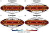 |
Fig. 21 Plasma flow (color surfaces 10−16 kg m−3) at R∕RE = 2.75 for ICMEs that impacted Earth on (a) 31∕03∕2001b, (b) 24∕11∕2001, (c) 15∕05∕2005, and (d) 24∕08∕2005. Velocity isocontours at 50 km s−1 (light cyan), 100 km s−1 (yellow), 150 km s−1 (orange), and 200 km s−1 (red). |
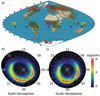 |
Fig. 22 (a) OCB line calculated from the 27∕05∕2017 ICME simulation. Energy flux calculated by Ovation prime simulations at the (b) North Hemisphere and (c) South Hemisphere. Ovation prime data are provided by the iSWA (iSW 2020). |
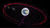 |
Fig. 23 Schematic view of the satellites at geosynchronous, high, medium, and low orbits around the Earth between 2000–2020. The orbits highlighted by red dots are geosynchronous satellites. The solid pink lines indicate orbits at R∕RE = i with i an integer between 2 to 8 (Ri). The dashed pink line indicates the geosynchronous orbit (Rg). The colored symbols and horizontal lines show the standoff distance of the magnetopause and the BS nose for the different ICMEs we analyzed: light green star for 22∕10∕1999, light cyan star for 16∕07∕2000, light pink star for 31∕03∕2001b, light gray star for 24∕11∕2001, yellow diamond for 29∕05∕2003, cyan diamond for 24∕10∕2003, pink diamond for 07∕11∕2004, gray diamond for 21∕01∕2005, orange triangle for 15∕05∕2005, and blue triangle for 24∕08∕2005. |
5 Discussion and conclusions
The distortion induced by the SW and the IMF on the topology of the Earth magnetosphere must be analyzed in detail because the large variability of the space weather conditions triggers a wide number of physical phenomena, for example, geomagnetic storms. Extreme space weather conditions have consequences for the integrity of satellites orbiting the Earth, electric power grids, and human health. In addition, an efficient shielding of the exoplanet magnetic field to avoid the direct precipitation of the stellar wind toward the surface is critical for exoplanet habitability.
Simulating the interaction of the SW and IMF with the Earth magnetic field using MHD models is a useful tool for analyzing the global structures of the magnetosphere during different space weather conditions. The validity of the MHD models was confirmed by comparing simulation results and spacecraft- and ground-based measurements (Watanabe & Sato 1990; Raeder et al. 2001; Wang et al. 2003a; Facskó et al. 2016; Honkonen et al. 2013). Consequently, a parametric analysis based on MHD simulations regarding the SW density, velocity, and temperature as well as the IMF orientation and intensity may provide a reasonable first approximation of the space weather effects on the topology of the Earth magnetosphere. We recall that no kinetic effects are included in the study, thus deviations between simulation results and observational data can exist for some of the extreme space weather configurations we analyzed.
The set of simulations we performed for which we fixed the SW dynamic pressure, but modified the IMF orientation and intensity show the critical role of the IMF on the topology of the Earth magnetosphere. It leads to a large variation in the magnetopause standoff distance, the location of the reconnection regions between the IMF and the Earth magnetic field where the SW is injected inside the inner magnetosphere, the plasma streams between the magnetosheath and the Earth surface as well as the open and closed field line boundary. Particularly the southward, Sun–Earth, and Earth–Sun IMF orientations lead to the smallest magnetopause standoff distances as the IMF intensity increases. In addition, the reconnection regions are closer to the Earth surface as the IMF intensity increases, although at different locations inside the magnetosphere regarding the IMF orientation. This modifies the plasma flows toward the Earth surface. In the same way, an intense IMF oriented in the southward direction causes a decrease in latitude of the OCB, exposing wider regions of the Earth surface to the plasma flows along the magnetic field lines. For example, the OCB on the DS (0° longitude) decreases from 72 to 53° when simulations without an IMF and with a southward IMF with 250 nT are compared. The results of the parametric study are consistent with those of other authors regarding the magnetopause standoff distance (Song et al. 1999; Kabin et al. 2004; Lavraud & Borovsky 2008; Ridley et al. 2010; Meng et al. 2012; Wang et al. 2015) and the latitude of the OCB (Lopez et al. 1999; Kabin et al. 2004; Wild et al. 2004; Rae et al. 2004; Wang et al. 2016; Burrell et al. 2020).
The simulations indicate that the direct precipitation of the SW toward the Earth surface is very unlikely in the range of space weather conditions expected for current and future stages of the Sun in the main-sequence evolution. The extreme space weather conditions during ICME and super-ICME impacting the Earth cannot lead to a compression and erosion of the Earth magnetosphere that would be large enough to reduce the magnetosphere standoff distance below Rsd ∕RE = 1. For example, the SW precipitation toward the Earth surface for an IMF that is purely oriented in the southward direction requires an IMF intensity of 1000 nT and a SW dynamic pressure above 350 nPa, space weather conditions well above super-ICMEs. In addition, if the analysis is extended to previous stages of the solar evolution, the simulations show an efficient shielding of the Earth surface 1100 Myr after the Sun enters the main sequence. On the other hand, early evolution stages when the solar rotation rate was 5–10 times faster than the current rotation rate, the case of the first 440 Myr of the solar main sequence, the Earth habitability could be threatened during extreme space weather conditions. These results are consistent with the studies of See et al. (2014); Airapetian (2016). The Earth magnetic field intensity is a fixed parameter in the analysis, although several studies indicated that the Earth magnetic field might be stronger during early evolution phases of the solar system (Tarduno et al. 2007, 2010, 2020). In addition, there are other factors that affect the young Earth habitability that we did not include in the study, for example, the solar luminosity and X-ray or ultraviolet emission (Cockell 2001; Sackmann & Boothroyd 2003; Ribas et al. 2005; Cnossen et al. 2007) or the atmospheric evolution (Kasting & Catling 2003; Arndt & Nisbet 2012; Gronoff et al. 2020). Consequently, supplementary analyses are required to confirm the habitability of the young Earth. This will be the topic for a future research.
An ICME classification for the Earth is proposed regarding the SW dynamic pressure, IMF intensity, and Disturbance Storm Time Index. The ICME classification consists of three categories: common, strong, and super-ICMEs. Common ICMEs have a relatively fast recurrence and cover the main number of extreme space weather events impacting the Earth with SW dynamic pressures < 40 nPa, IMF intensities <50 nT, and Dst < −100 nT. Strong ICMEs have a lower recurrence, a few events each year, particularly associated with the maximum of the solar magnetic activity cycle, showing a dynamic pressure in the range of [40, 100] nPa, an IMF intensity of [50, 100] nT, and Dst = [−100, −500] nT. The super-ICME category identifies events that occur once per century, similar to the Carrington event with an SW dynamic pressure above 100 nPa, an IMF intensity above 100 nT, and Dst > −500 nT. This classification is consistent with those in the studies of other authors (Rastatter et al. 2002; Tsurutani et al. 2003; Siscoe et al. 2006; Saiz et al. 2008; Balan et al. 2014; Keika et al. 2015).
The simulations we performed to reproduce the effect of the ICMEs impacting the Earth between 1997 − 2020 indicate that all the events can be included in the common ICME category, except for the extreme space weather conditions observed on 16∕07∕2000 and 24∕11∕2001. These are classified as close to the strong ICME category (Pd ≈ 30 nPa and |B|IMF ≈ 50 nT). The event on 29∕10∕2003 was not included in the study because of the lack of SW and IMF data, although this event probably belongs to the strong ICME category (Balan et al. 2014). For example, the Earth magnetosphere distortion during the 24∕11∕2001 ICME was large enough to potentially impact the electric grids of the North of Canada, Alaska, the North of Russia, and the Nordic countries (except for continental Denmark). In addition, the Kp = 8 index calculated regarding the plasma flows toward the Earth surface is the same as the Kp = 8 index we measured.
We recall that the simulations neglect the effect imprinted on the Earth magnetosphere by previous space weather conditions. Consequently, the simulations performed for ICMEs showing a fast variation in space weather conditions could overestimate the forcing of the SW and IMF. This is the case of the simulations performed for the 31∕03∕2001 ICME; see Fig. D.2. It shows large variations in IMF orientation and intensity as well as SW dynamic pressure within a time frame of minutes. On the other hand, the space weather parameters are quasi-steady within a time frame of 1 h during the 15∕05∕1997 ICME; see Fig. D.1. The simulation results are therefore more accurate.
Although no direct SW precipitation is expected toward the Earth surface, extreme space weather conditions can endanger the integrity of the satellites around the Earth because the magnetopause standoff distance decreases and the satellite orbit on the Earth DS is partially unprotected outside the magnetosphere. Southward and ecliptic IMF orientations are particularly adverse for geosynchronous satellites, which are partially exposed to the SW if the SW dynamic pressure is ≈ 14–26 nPa and the IMF intensity 10 nT, that is to say, 5–10 times the dynamic pressure of regular space weather conditions. On the other hand, medium-orbit satellites at 20 000 km are directly exposed to the SW during common ICMEs if the IMF orientation is southward and during strong ICMEs if the IMF orientation is Earth–Sun or ecliptic. In the same way, medium-orbit satellites at 10 000 km are directly exposed to the SW if a super-ICME with a southward IMF orientation impacts the Earth. For example, during the ICMEs on 15∕07∕2000, 24∕11∕2001, 29∕05∕2003, and 21∕01∕2005, the geosynchronous satellites were directly affected by the SW during a fraction of the orbit on the Earth DS, although medium-orbit satellites below R∕RE ≈ 5 were protected by the magnetosphere during the full orbit. Other important threats to the satellite integrity during extreme space weather conditions, such as the enhancement of the Earth radiation belts and the atmosphere drag force, are not included in the study.
Acknowledgements
This work was supported by the project 2019-T1/AMB-13648 founded by the Comunidad de Madrid. The research leading to these results has received funding from the grants ERC WholeSun 810218, Exoplanets A and INSU/PNP. We extend our thanks to CNES for Solar Orbiter, PLATO and Meteo Space science support and to INSU/PNST for their financial support. This work has been supported by Comunidad de Madrid (Spain) – multiannual agreement with UC3M (“Excelencia para el Profesorado Universitario” – EPUC3M14) – Fifth regional research plan 2016–2020. Data available on request from the authors. The authors acknowledge the Community Coordinated Modeling Center (CCMC) and the main developer of Ovation prime code Prof. Patrick Newell. The authors also acknowledge J. Reynolds and V. Trivaldos for managing the Uranus cluster in Carlos III University where the simulations for this study were performed.
Appendix A Upper ionosphere model
The upper ionospheric domain is located between R = 2 − 2.5RE in simulations with Pd > 1 nPa and between R = 3 − 3.5RE in simulations with Pd < 1 nPa. The upper ionosphere model is based on (Büchner et al. 2003). Below the lower boundary of the upper ionosphere, the magnetic field intensity is too high, thus the simulation time step is too small. In addition, a single-fluid MHD model cannot correctly reproduce magnetosphere regions such as the inner ionosphere or the plasma sphere because the kinetic effects are strong.
First, the field-aligned current (JFAC) is calculatedas
 (A.1)
(A.1)
with J the plasma current, J⊥ the perpendicular component of the plasma current along the magnetic field line, mu0 the vacuum magnetic permeability, and B the magnetic field.
Next, the electric field of the upper ionosphere model is calculated using the Pedersen conductance (σ) empirical formula,
 (A.4)
(A.4)
with E0 = KBTe the mean energy of the electrons,  the energy flux, and KB the Boltzmann constant (Te and me are the electron temperature and mass, respectively). Thus, the electric field (E) linked to the FAC is
 (A.5)
(A.5)
When the electric field is calculated, the velocity of the plasma in the upper ionosphere is
 (A.6)
(A.6)
The plasma density in the upper ionosphere is defined with respect to the Alfvén velocity. The module of the Alfvén velocity is fixed (vA = 8 ⋅ 103 km/s) to control the simulation time step, thus the density profile between R = 2 − 2.5RE does not evolve during the simulation, defined as
 (A.7)
(A.7)
The plasma pressure in the upper ionosphere model is defined with respect to the sound speed of the SW (csw) and at the inner boundary (cp),
 (A.8)
(A.8)
with γ = 5∕3 the polytropic index,  with Tp is the plasma temperature at the inner boundary, and
  with Tsw the SW temperature. Figure C.1 shows the profiles of the density and pressure inside the upper ionosphere model for the simulation with Tsw = 1.8 ⋅ 105 K, n = 20 cm−3, |v| = 350 km/s, and |B|IMF = 0.
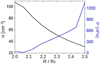 |
Fig. A.1 Radial profiles of the density and pressure inside the upper ionosphere model. Simulation with Tsw = 1.8 ⋅ 105 K, n = 20 cm−3, |v| = 350 km/s, and |B|IMF = 0. |
The initial model conditions for the plasma density and pressure are defined to have a smooth transition between the upper ionosphere and the simulation domains. During the simulation, the pressure and density gradients increased because the density and pressure profiles were fixed inside the inner ionosphere, but evolved freely in the simulation domain. The answer of the system during the early stages of the simulation is to compensate for the gradients feeding plasma toward the simulation domain, generating an outward plasma flux that saturates when the inner magnetosphere reaches the steady state. Henceforth, the plasma flows are dominated by the balance between the SW injection inside the inner magnetosphere and the plasma streams toward the planet surface.
The numerical model we used to study space weather configurations with low SW dynamic pressure, Pd ≤ 1 nPa, was modified with respect to high Pd simulations. The inner boundary was located at Rin = 3RE and the upper ionosphere domain between 3.0 − 3.5RE. The reason for this modification was that we wished to avoid an overestimation of the magnetosphere thermal pressure in low Pd simulations. This can be caused by the plasma Alfvén velocity that is imposed in the upper ionosphere, which is required to control the simulation time step and may lead to an artificial enhancement of the plasma fluxes toward the simulation domain. This numerical issue was avoided by displacing the inner boundary of the model outward. This reduced the fluxes and minimized the overestimation of the magnetosphere thermal pressure. For high Pd simulations, the effect of outward fluxes is negligible in the pressure balance.
The model prediction for quite space weather conditions was compared with the analysis of Samsonov et al. (2016) by performing a simulation using the same parameters as in the original benchmark study: n = 5 cm−3, Vx = −400 km/s, T =2 ⋅ 105 K, By = −Bx = 3.5 nT, and Bz = 0 nT. The location of the magnetopause is Rx∕RE = 10.7, Ry ∕RE = 16.8, R−y ∕RE = 16.6, and Rz ∕RE = 14.9. The model prediction and the benchmark study agree reasonably well. Figure A.2 shows the electric field in the simulation domain. The local maximum of the electric field is also consistent with the simulations in Samsonov et al. (2016) near the BS (fig 1). There is a secondary local maximum of the electric field module near the lower boundary of the simulation domain that is caused by the conditions imposed in the upper ionosphere. The module of the electric field predicted inside the magnetosphere is similar to Cluster spacecraft observations during the magnetopause crossing on 30∕02∕2002 (De Keyser et al. 2005). The electric field measured in the current sheet and magnetosheath is one order of magnitude higher than the simulations because the IMF module is 10 times larger during the Cluster magnetopause crossing. When the simulation was performed using a southward IMF with |B| = 50 nT and Pd = 5 nPa, similar to the space weather conditions during Cluster magnetopause crossing, the predicted electric field is 15 − 30 mV/m in the current sheet and magnetosheath region. This is similar to Cluster spacecraft observations.
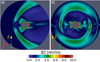 |
Fig. A.2 Electric field module in the simulation domain for the benchmark case in Samsonov et al. (2016) in (a) the XZ plane and (b) in the YZ plane. |
In addition, another two simulations were performed using the same SW parameters, but for northward and southward IMF orientations with |Bz| = 3 nT, identifying the displacement of the magnetopause location defined as ΔR∕RE = northward(R)∕RE − southward(R)∕RE: ΔRx∕RE = 0.2, ΔRy∕RE = 0.1 and ΔRz∕RE = −1.0. Again, thereis a reasonable agreement.
Next, the model was compared with the Carrington-like event analyzed by Ridley et al. (2006), who identified a magnetopause standoff distance of R∕RE = 2 (equal to the lower boundary of the simulation domain) for the parameters n = 750 cm−3, Vx = −1600 km/s (Pd = 1600 nPa), T =3.5 ⋅ 107 K, Bx = 150 nT, By = 170 nT, and Bz = 200 nT. Our model cannot be used to simulate space weather conditions leading to a magnetopause standoff distance smaller R∕RE = 2.5, although the extrapolation of the modelresults predicts R∕RE ≈ 1.22 if Pd = 1600 nPa and Bz = 200 nT (pure southward IMF orientation).
The electric field in the upper ionosphere domain remains almost unchanged during the simulation because the density profile was fixed. Figure A.3 panel a shows the radial electric field inside the upper ionosphere (North hemisphere at R∕RE = 3.1) for the Samsonov et al. (2016) benchmark case, indicating a reasonable order-of-magnitude agreement with respect to other models and satellite measurements (Shume et al. 2009; Alken & Maus 2010; Watanabe et al. 2014). Panel b indicates the FAC intensity and orientation, values in the range of the observations and modeling data (from nA∕m2 to several μAm2 regarding the space weather conditions) Weimer (2001); Waters et al. (2001); Ritter et al. (2013); Bunescu et al. (2019); Zhang et al. (2020).
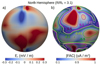 |
Fig. A.3 (a) Radial electric field and (b) FAC intensity in the North Hemisphere at R∕RE = 3.1 for the Samsonov et al. (2016) benchmark case. The colored isocontours indicate different FAC intensities and inward and outward (green and pink) orientations. |
Appendix B Magnetic field line mapping
The magnetic field lines of the simulations were mapped with respect to the magnetic field of an unperturbed dipole. To this end, a simulationwithout the driving effect of the SW and IMF was performed in which we decreased the inner boundary of the simulation domain to R∕RE = 1. Figure B.1 shows the mapping of the magnetic field lines for simulations during regular and extreme space weather conditions with the magnetic field of an unperturbed dipole.
The mapping shows that even for simulations with a high dynamic pressure (panel b) and |B|IMF (panel c), the magnetic field lines follows the unperturbed dipole magnetic field lines inside the computational domain of the upper ionosphere, between R∕RE = 2 to 2.5, indicated in the figures by the dashed and dotted white line. Consequently, the extrapolations of the OCB line and plasma flows toward the Earth surface are reasonably accurate.
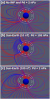 |
Fig. B.1 3D view of the magnetic field line mapping between an unperturbed dipole and simulations with (a) no IMF and Pd = 2 nPa, (b) Sun-Earth IMF |B|IMF = 10 nT and Pd = 105 nPa, and (c) Sun-Earth IMF |B|IMF = 100 nT and Pd = 2 nPa. The dashed white line indicates the inner boundary of the simulation domain (R∕RE = 2), and the dotted white line shows the upper boundary of the ionosphere model (R∕RE = 2.5). The red lines show the magnetic field lines in the simulation with only the dipole magnetic field and the blue lines the magnetic field lines in the simulation with dipole + IMF magnetic fields. |
Appendix C Magnetotail and OCB line latitude on the nightside
The simulation outer boundary is located at R∕RE = 30, although themagnetotail extension can exceed R∕RE = 30, thus this magnetosphere structure is only partially reproduced by the model. Consequently, the last close magnetic field line cannot be accurately identified on the Earth NS, and this also holds for the latitude of the OCB line. This is the case for the simulations with Pd≥ 85 nPa and |BIMF|≤ 10 nT. Therefore the analysis of the OCB line latitude on the NS was not performed for these configurations. Nevertheless, the outer boundary conditions might affect the magnetotail topology when the simulation reaches steady state. Figure C.1 compares the magnetotail structure in simulations for the same space weather conditions, but increasing the outer boundaries from R∕RE = 30 to 100.
The simulations with the outer boundary at R∕RE = 30 and 100 agree well regarding the Earth magnetic field on the DS and NS, indicating that the outer boundary conditions have a negligible effect on thecomputational domain. Consequently, the location of the last close magnetic field lines on the NS is similar, leading to values of the OCB line latitude inside the uncertainty of the model resolution.
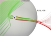 |
Fig. C.1 Polar plot of the magnetic field lines in simulations with the outer boundary at R∕RE= 30 (red line) and 100 (green line) for the 27∕05∕2017 ICME. The gray sphere indicates the outer boundary of the simulation with at R∕RE= 30. |
Appendix D CME list
Table D.1 shows the SW density, temperature, radial velocity, dynamic pressure, IMF components, and module as well as the data source for the CME subsample.
The simulation inputs were obtained from OMNIWeb (OMN 2020), ACE SWICS (ACE 2020), and DSCOVR (DSC 2020) after the front of the ICME impacted the Earth. OMNIWeb pro- vides high-resolution OMNI (HRO) data based on the Global Geospace Science (GGS) Wind satellite (Ogilvie & Desch 1997), ACE SWICS data from the Advanced Composition Explorer (ACE) spacecraft (Stone et al. 1998), and DSCOVR data from the Deep Space Climate Observatory (Burt & Smith 2012). The strong CME impacting the Earth on 29∕10∕2003 is not included in the list because no data for the SW density and temperature nor for the IMF module and intensity are available.
Figures D.1 and D.2 show two examples of the space weather condition obtained from OMNIWeb. We used them as input for the simulations for the ICMEs on 15∕05∕1997 and 31∕03∕2001, respectively.
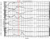 |
Fig. D.1 OMNIWeb data during the 15∕05∕1997 ICME. (a) |B| (nT), (b) Bx (nT), (c) By (nT), (d) Bz (nT), (e) |v| (km/s), (f) vr (km/s), (g) n (cm−3), and (h) T (104 K). The solid red line indicates the time frame we selected as the simulation input. |
SW and IMF parameters of the CME selection between 1997 − 2020. Date (first column), SW density (second column), SW temperature (third column), SW radial velocity (fourth column), SW dynamic pressure (fifth column), IMF component along the Sun–Earth direction (sixth column), IMF component along the magnetic axis direction (seventh column), IMF component along the ecliptic direction (eighth column), IMF module (ninth column), data source (tenth column), and measured Kp index (eleventh column).
 |
Fig. D.2 OMNIWeb data during the 31∕03∕2001 ICME. (a) |B| (nT), (b) Bx (nT), (c) By (nT), (d) Bz (nT), (e) |v| (km/s), (f) vr (km/s), (g) n (cm−3), and (h) T (104 K). The solid red line indicates the time frame we selected as the simulation input. |
Appendix E Acronym list
Acronym list.
Appendix F Parameter list for the simulations
The SW and IMF parameters in the simulations included in figures 6, 10, 11, 12, 13, 14, and 15 are (for Sun–Earth, Earth–Sun, northward, southward and ecliptic ctr-clockwise IMF orientations) listed below.
The SW and IMF parameters in the simulations included in figures 8 and 9, for which we fixed the SW velocity and temperature are (for the Sun–Earth IMF orientation) listed below
The SW and IMF parameters in the simulations included in the figures 8 and 9, for which we fixed the SW density and temperature are (for the Sun-Earth IMF orientation) listed below.
The SW and IMF parameters in the simulations included in figure 9 fixing the SW density and velocity are (for the Sun–Earth IMF orientation) listed below.
The SW and IMF parameters in the simulations included in the figures 16 and 17, for which we fixed the SW density and temperature are (for Earth–Sun, northward, southward, and ecliptic ctr-clockwise IMF orientations) listed below.
References
- ACE 2020, ACE SWICS 1.1 Level 2 Data http://www.srl.caltech.edu/ACE/ASC/level2/lvl2DATA_SWICS-SWIMS.html [Google Scholar]
- Acuña, M. H., Ogilvie, K. W., Baker, D. N., et al. 1995, Space Sci. Rev., 71, 5 [Google Scholar]
- Ahuir, J., Brun, A. S., & Strugarek, A. 2020, A&A, 635, A170 [NASA ADS] [CrossRef] [EDP Sciences] [Google Scholar]
- Airapetian, V. S. 2016, Proc. Int. Astron. Union, 12, 315 [NASA ADS] [CrossRef] [Google Scholar]
- Airapetian, V. S., Glocer, A., & Danchi, W. 2015a, 18th Cambridge Workshop on Cool Stars, Stellar Systems, and the Sun, Proc. of the conference held at Lowell Observatory, 8-14 June, 2014, eds. G. van Belle & H.C. Harris., 257 [Google Scholar]
- Airapetian, V., Glocer, A., & Guillaume, G. 2015b, Proc. Int. Astron. Union, 11, 409 [CrossRef] [Google Scholar]
- Airapetian, V. S., Barnes, R., Cohen, O., et al. 2020, Int. J. Astrobiol., 19, 136 [NASA ADS] [CrossRef] [Google Scholar]
- Aizawa, S., Griton, L. S., Fatemi, S., et al. 2021, Planet. Space Sci., 198, 105176 [NASA ADS] [CrossRef] [Google Scholar]
- Alken, P., & Maus, S. 2010, J. Atmos. Sol-Terr. Phys., 72, 319 [NASA ADS] [CrossRef] [Google Scholar]
- Andréeová, K., Pulkkinen, T. I., Laitinen, T. V., & Přech, L. 2008, J. Geophys. Res.: Space Phys., 113, A09224 [Google Scholar]
- Arndt, N. T., & Nisbet, E. G. 2012, Annu. Rev. Earth Planet. Sci., 40, 521 [NASA ADS] [CrossRef] [Google Scholar]
- Baker, D. N., Pulkkinen, T. I., Büchner, J., & Klimas, A. J. 1999, J. Geophys. Res.: Space Phys., 104, 14601 [NASA ADS] [CrossRef] [Google Scholar]
- Baker, D. N., Li, X., Pulkkinen, A., et al. 2013, Space Weather, 11, 585 [NASA ADS] [CrossRef] [Google Scholar]
- Balan, N., Skoug, R., Tulasi Ram, S., et al. 2014, J. Geophys. Res.: Space Phys., 119, 10, 041 [NASA ADS] [Google Scholar]
- Bazilevskaya, G. A. 2005, Adv. Space Res., 35, 458 [NASA ADS] [CrossRef] [Google Scholar]
- Borovsky, J. E., Hesse, M., Birn, J., & Kuznetsova, M. M. 2008, J. Geophys. Res.: Space Phys., 113, A07210 [Google Scholar]
- Borovsky, Joseph E., & Shprits, Y. Y. 2017, J. Geophys. Res.: Space Phys., 122, 11543 [NASA ADS] [Google Scholar]
- Boroyev, R. N., Vasiliev, M. S., & Baishev, D. G. 2020, J. Atmos. Sol.-Terr. Phys., 204, 105290 [NASA ADS] [CrossRef] [Google Scholar]
- Büchner, J., Dum, C., & Scholer, M. 2003, Space Plasma Simulation (Berlin, Heidelberg: Springer-Verlag) [CrossRef] [Google Scholar]
- Bunescu, C., Vogt, J., Marghitu, O., & Blagau, A. 2019, Ann. Geophys., 37, 347 [NASA ADS] [CrossRef] [Google Scholar]
- Burch, J. L., & Phan, T. D. 2016, Geophys. Res. Lett., 43, 8327 [NASA ADS] [CrossRef] [Google Scholar]
- Burrell, A. G., Chisham, G., Milan, S. E., et al. 2020, Ann. Geophys., 38, 481 [NASA ADS] [CrossRef] [Google Scholar]
- Burt, J., & Smith, B. 2012, in 2012 IEEE Aerospace Conference, 1 [Google Scholar]
- Cairns, Iver H., & Lyon, J. G. 1995, J. Geophys. Res.: Space Phys., 100, 17173 [NASA ADS] [CrossRef] [Google Scholar]
- Cairns, Iver H., & Lyon, J. G. 1996, Geophys. Res. Lett., 23, 2883 [NASA ADS] [CrossRef] [Google Scholar]
- Cane, H. V., & Richardson, I. G. 2003, J. Geophys. Res.: Space Phys., 108, 1 [Google Scholar]
- Cane, H. V., Richardson, I. G., & St. Cyr, O. C. 2000, Geophys. Res. Lett., 27, 3591 [NASA ADS] [CrossRef] [Google Scholar]
- Cannon, P., Angling, M., Barclay, L., et al. 2013, Extreme space weather: impacts on engineered systems and infrastructure, Tech. rep. [Google Scholar]
- Carolan, S., Vidotto, A., Loesch, C., & Coogan, P. 2019, MNRAS, 489, 5784 [NASA ADS] [CrossRef] [Google Scholar]
- Carrington, R. C. 1859, MNRAS, 20, 13 [NASA ADS] [CrossRef] [Google Scholar]
- Chane, E., Raeder, J., Saur, J., et al. 2015, J. Geophys. Res.: Space Phys., 120, 8517 [NASA ADS] [CrossRef] [Google Scholar]
- Chane, E., Saur, J., Neubauer, F. M., Raeder, J., & Poedts, S. 2012, J. Geophys. Res.: Space Phys., 117, A09217 [Google Scholar]
- Chaston, C. C., Yao, Y., Lin, N., Salem, C., & Ueno, G. 2013, J. Geophys. Res.: Space Phys., 118, 5579 [NASA ADS] [CrossRef] [Google Scholar]
- Chen, C. H. K., & Boldyrev, S. 2017, ApJ, 842, 122 [NASA ADS] [CrossRef] [Google Scholar]
- Chen, S-H, Le, G, & Fok, M-C. 2015, J. Geophys. Res.: Space Phys., 120, 113 [NASA ADS] [CrossRef] [Google Scholar]
- Chen, Y., Tóth, G., Cassak, P., et al. 2017, J. Geophys. Res.: Space Phys., 122, 10, 318 [NASA ADS] [Google Scholar]
- Cherniak, I., & Zakharenkova, I. 2018, Space Weather, 16, 1377 [CrossRef] [Google Scholar]
- Choi, H.-S., Lee, J., Cho, K.-S., et al. 2011, Space Weather, 9, S06001 [Google Scholar]
- Cliver, E. W., Feynman, J., & Garrett, H. B. 1990, J. Geophys. Res.: Space Phys., 95, 17103 [NASA ADS] [CrossRef] [Google Scholar]
- Cnossen, I., Favata, J., Witasse, F., et al. 2007, J. Geophys. Res.: Planets, 112, E02008 [CrossRef] [Google Scholar]
- Cockell, C. S. 2001, Ultraviolet Radiation and Exobiology (Blaustein A. R. Springer) [CrossRef] [Google Scholar]
- Daglis, I. A. 2006, Space Sci Rev., 124, 183 [Google Scholar]
- De Keyser, J., Dunlop, M. W., & Owen, C. J. 2005, Space Sci Rev., 118, 231 [NASA ADS] [CrossRef] [Google Scholar]
- De Zeeuw, D. L., Sazykin, S., Wolf, R. A., et al. 2004, J. Geophys. Res.: Space Phys., 109, A12219 [CrossRef] [Google Scholar]
- Dedner, A., Kemm, F., Kröner, D., et al. 2002, J. Comput. Phys., 175, 645 [Google Scholar]
- Den, M., Tanaka, T., Fujita, S., et al. 2006, Space Weather, 4, S06004 [Google Scholar]
- Dmitriev, A. V., Lin, R. L., Liu, S. Q., & Suvorova, A. V. 2016, Space Weather, 14, 530 [CrossRef] [Google Scholar]
- DSC 2020, DSCOVR Space Weather Data Portal https://www.ngdc.noaa.gov/dscovr/portal/index.html [Google Scholar]
- Dusik, S., Granko, G., Safránková, J., Nĕmecek, Z., & Jelinek, K. 2010, Geophys. Res. Lett., 37, L19103 [Google Scholar]
- Eastwood, J. P., Sibeck, D. G., Angelopoulos, V., et al. 2008, Geophys. Res. Lett., 35, L17S03 [NASA ADS] [CrossRef] [Google Scholar]
- Eastwood, J. P., Hietala, H., Toth, G., Phan, T. D., & Fujimoto, M. 2015, Space Sci. Rev., 188, 251 [CrossRef] [Google Scholar]
- Eastwood, J. P., Biffis, E., Hapgood, M. A., et al. 2017, Risk Anal., 37, 206 [NASA ADS] [CrossRef] [Google Scholar]
- Eastwood, J. P., Hapgood, M. A., Biffis, E., et al. 2018, Space Weather, 16, 2052 [NASA ADS] [CrossRef] [Google Scholar]
- Emeriau-Viard, C., & Brun, S. 2017, ApJ, 846, 26 [NASA ADS] [CrossRef] [Google Scholar]
- Escoubet, C. P., Fehringer, M., & Goldstein, M. 2001, Ann. Geophys., 19, 1197 [NASA ADS] [CrossRef] [Google Scholar]
- Fabbian, D., Simoniello, R., Collet, R., et al. 2017, Astron. Nachr., 338, 753 [NASA ADS] [CrossRef] [Google Scholar]
- Facskó, G., Honkonen, I., Zivković, T., et al. 2016, Space Weather, 14, 351 [CrossRef] [Google Scholar]
- Folsom, C. P., Bouvier, J., Petit, P., et al. 2017, MNRAS, 474, 4956 [Google Scholar]
- Fuselier, S. A., Lewis, W. S., Schiff, C., et al. 2016, Space Sci. Rev., 199, 77 [CrossRef] [Google Scholar]
- Gallet, F., Charbonnel, C., Amard, L., et al. 2017, A&A, 597, A14 [NASA ADS] [CrossRef] [EDP Sciences] [Google Scholar]
- Ganushkina, N., Jaynes, A., & Liemohn, M. 2017, Space Sci. Rev., 212, 1315 [CrossRef] [Google Scholar]
- Garraffo, C., Drake, J. J., & Cohen, O. 2016, ApJ, 833, L4 [NASA ADS] [CrossRef] [Google Scholar]
- Gombosi, T. I. 1994, Gaskinetic Theory, Cambridge Atmospheric and Space Science Series (Cambridge University Press) [Google Scholar]
- Gonzalez, W. D., Joselyn, J. A., Kamide, Y., et al. 1994, J. Geophys Res.: Space Phys., 99, 5771 [NASA ADS] [CrossRef] [Google Scholar]
- González Hernández, I., Komm, R., Pevtsov, A., & Leibacher, J. 2014, Solar Origins of Space Weather and Space Climate (New York: Springer-Verlag) [Google Scholar]
- Gosling, J. T. 1990, Coronal Mass Ejections and Magnetic Flux Ropes in Interplanetary Space (American Geophysical Union (AGU)), 343 [Google Scholar]
- Gosling, J. T., McComas, D. J., Phillips, J. L., & Bame, S. J. 1991, J. Geophys. Res.: Space Phys., 96, 7831 [NASA ADS] [CrossRef] [Google Scholar]
- Greenwald, R. A., Baker, K. B., Dudeney, J. R., et al. 1995, Space Sci. Rev., 71, 761 [CrossRef] [Google Scholar]
- Gronoff, G., Arras, P., Baraka, S., et al. 2020, J. Geophys. Res.: Space Phys., 125, e2019JA027639 [Google Scholar]
- Grygorov, K., Safránková, J., Nĕmecek, Z., et al. 2017, Planet. Space Sci., 148, 28 [NASA ADS] [CrossRef] [Google Scholar]
- Hapgood, M. 2019, Space Weather, 17, 950 [NASA ADS] [CrossRef] [Google Scholar]
- Hayakawa, H., Ebihara, Y., Hand, D. P., et al. 2018, ApJ, 869, 57 [NASA ADS] [CrossRef] [Google Scholar]
- Honkonen, I., Rastätter, L., Grocott, A., et al. 2013, Space Weather, 11, 313 [NASA ADS] [CrossRef] [Google Scholar]
- Howard, R. A. 2006, A Historical Perspective on Coronal Mass Ejections (American Geophysical Union (AGU)), 7 [Google Scholar]
- Howard, T. 2014, Space Weather and Coronal Mass Ejections (New York: Springer-Verlag) [CrossRef] [Google Scholar]
- Hu, Y.-Q., Guo, X.-C., Li, G.-Q., Wang, C., & Huang, Z.-H. 2005, Chinese Phys. Lett., 22, 2723 [Google Scholar]
- Hudson, M. K., Elkington, S. R., Lyon, J. G., et al. 1997, J. Geophys. Res.: Space Phys., 102, 14087 [NASA ADS] [CrossRef] [Google Scholar]
- Huttunen, K., Koskinen, H. E. J., Pulkkinen, T. I., et al. 2002, J. Geophys. Res.: Space Phys., 107, 1440 [NASA ADS] [CrossRef] [Google Scholar]
- Ilie, R., Liemohn, M. W., Toth, G., & Skoug, R. M. 2012, J. Geophys. Res.: Space Phys., 117, A04208 [Google Scholar]
- iSW 2020, iNTEGRATED SPACE WEATHER ANALYSIS SYSTEM https://iswa.ccmc.gsfc.nasa.gov/IswaSystemWebApp/ [Google Scholar]
- Jakosky, B. M., Grebowsky, J. M., Luhmann, J. G., & Brain, D. A. 2015, Geophys. Res. Lett., 42, 8791 [NASA ADS] [CrossRef] [Google Scholar]
- Janhunen, P., Palmroth, M., Laitinen, T., et al. 2012, J. Atmos. Sol.-Terr. Phys., 80, 48 [NASA ADS] [CrossRef] [Google Scholar]
- Jia, X., Slavin, J. A., Gombosi, T. I., et al. 2015, J. Geophys. Res. (Space Phys.), 120, 4763 [NASA ADS] [CrossRef] [Google Scholar]
- Jordanova, V. K., Yu, Y., Niehof, J. T., et al. 2014, Geophys. Res. Lett., 41, 2687 [NASA ADS] [CrossRef] [Google Scholar]
- Kabin, K., Gombosi, T. I., DeZeeuw, D. L., & Powell, K. G. 2000, Icarus, 143, 397 [NASA ADS] [CrossRef] [Google Scholar]
- Kabin, K., Rankin, R., Rostoker, G., et al. 2004, J. Geophys. Res.: Space Phys., 109, A05222 [NASA ADS] [CrossRef] [Google Scholar]
- Kabin, K., Heimpel, M. H., Rankin, R., et al. 2008, Icarus, 195, 1 [NASA ADS] [CrossRef] [Google Scholar]
- Kasting, J. F.,& Catling, D. 2003, ARA&A, 41, 429 [NASA ADS] [CrossRef] [Google Scholar]
- Katircioglu, F. T., Kaymaz, Z., Sibeck, D. G., & Dandouras, I. 2009, Ann. Geophys., 27, 3765 [NASA ADS] [CrossRef] [Google Scholar]
- Kay, C., Gopalswamy, N., Reinard, A., & Opher, M. 2017, ApJ, 835, 117 [NASA ADS] [CrossRef] [Google Scholar]
- Keika, K., Ebihara, Y., & Kataoka, R. 2015, Earth Planets Space, 67, 65 [NASA ADS] [CrossRef] [Google Scholar]
- Kidder, A., Winglee, R. M., & Harnett, E. M. 2008, J. Geophys. Res. (Space Phys.), 113, A09223 [Google Scholar]
- Kilpua, E. K. J., Lugaz, N., Mays, M. L., & Temmer, M. 2019, Space Weather, 17, 498 [NASA ADS] [CrossRef] [Google Scholar]
- Kress, B. T., Hudson, M. K., Looper, M. D., et al. 2007, J. Geophys. Res.: Space Phys., 112, A09215 [Google Scholar]
- Laitinen, T. V., Pulkkinen, T. I., Palmroth, M., Janhunen, P., & Koskinen, H. E. J. 2005, Ann. Geophys., 23, 3753 [NASA ADS] [CrossRef] [Google Scholar]
- Lavraud, B., & Borovsky, J. E. 2008, J. Geophys. Res.: Space Phys., 113, A00B08 [Google Scholar]
- Le, G., Luhr, H., Anderson, B. J., et al. 2016, Geophys. Res. Lett., 43, 2396 [NASA ADS] [CrossRef] [Google Scholar]
- Li, W., & Hudson, M. K. 2019, J. Geophys. Res.: Space Phys., 124, 8319 [NASA ADS] [CrossRef] [Google Scholar]
- Lin, Y., Wing, S., Johnson, J. R., et al. 2017, Geophys. Res. Lett., 44, 5892 [NASA ADS] [CrossRef] [Google Scholar]
- Linsky, J. 2019, Space Weather: The Effects of Host Star Flares on Exoplanets, 955 (Springer International Publishing), 229 [CrossRef] [Google Scholar]
- Liu, Y. D., Luhmann, J. G., Kajdic, P., et al. 2014, Nat. Commun., 5, 3481 [NASA ADS] [CrossRef] [Google Scholar]
- Liu, Z.-Q., Lu, J. Y., Wang, C., et al. 2015, J. Geophys. Res.: Space Phys., 120, 5645 [NASA ADS] [CrossRef] [Google Scholar]
- Loewe, C. A., & Prölss, G. W. 1997, J. Geophys. Res.: Space Phys., 102, 14209 [NASA ADS] [CrossRef] [Google Scholar]
- Lopez, R. E., Wiltberger, M., Lyon, J. G., Goodrich, C. C., & Papadopoulos, K. 1999, Geophys. Res. Lett., 26, 967 [NASA ADS] [CrossRef] [Google Scholar]
- Low, B. C. 2001, J. Geophys. Res.: Space Phys., 106, 25141 [NASA ADS] [CrossRef] [Google Scholar]
- Lu, S., Lu, Q., Lin, Y., et al. 2015, J. Geophys. Res.: Space Phys., 120, 6286 [NASA ADS] [CrossRef] [Google Scholar]
- Lugaz, N., Farrugia, C. J., Huang, C.-L., & Spence, H. E. 2015, Geophys. Res. Lett., 42, 4694 [NASA ADS] [CrossRef] [Google Scholar]
- Lugaz, N., Farrugia, C. J., Huang, C.-L., et al. 2016, Nat. Commun., 7, 13001 [NASA ADS] [CrossRef] [Google Scholar]
- Lundin, R., Lammer, H., & Ribas, I. 2007, Space Sci. Rev., 129, 245 [NASA ADS] [CrossRef] [Google Scholar]
- Lyon, J. G., Fedder, J. A., & Mobarry, C. M. 2004, J. Atmos. Sol.-Terr. Phys., 66, 1333 [NASA ADS] [CrossRef] [Google Scholar]
- Ma, Y.-J., Nagy, A. F., Toth, G., et al. 2007, Geophys. Res. Lett., 34, L24S10 [Google Scholar]
- Machol, J. L., Green, J. C., Redmon, R. J., Viereck, R. A., & Newell, P. T. 2012, Space Weather, 10, S03005 [Google Scholar]
- Manchester IV, Gombosi, T. I., Roussev, I., et al. 2004, J. Geophys. Res.: Space Phys., 109, A02107 [CrossRef] [Google Scholar]
- Manuzzo, R., Califano, F., Belmont, G., & Rezeau, L. 2020, Ann. Geophys., 38, 275 [NASA ADS] [CrossRef] [Google Scholar]
- Mays, M. L., Taktakishvili, A., Pulkkinen, A., et al. 2015, Sol. Phys., 290, 1775 [CrossRef] [Google Scholar]
- Mejnertsen, L., Eastwood, J. P., Hietala, H., Schwartz, S. J., & Chittenden, J. P. 2018, J. Geophys. Res.: Space Phys., 123, 259 [NASA ADS] [CrossRef] [Google Scholar]
- Meng, X., Toth, G., Liemohn, M. W., Gombosi, T. I., & Runov, A. 2012, J. Geophys. Res.: Space Phys., 117, A08216 [NASA ADS] [Google Scholar]
- Menvielle, M., & Berthelier, A. 1991, Rev. Geophys., 29, 415 [CrossRef] [Google Scholar]
- Mignone, A., Bodo, G., Massaglia, S., et al. 2007, ApJS, 170, 228 [Google Scholar]
- Mikhalev, A. V. 2019, Sol.-Terr. Phys., 5, 66 [NASA ADS] [Google Scholar]
- Molera Calvés, G., Pogrebenko, S. V., Cimò, G., et al. 2014, A&A, 564, A4 [NASA ADS] [CrossRef] [EDP Sciences] [Google Scholar]
- Moore, T. E., & Khazanov, G. V. 2010, J. Geophys. Res.: Space Phys., 115, A00J13 [CrossRef] [Google Scholar]
- Müller, J., Simon, S., Motschmann, U., et al. 2011, Comput. Phys. Commun., 182, 946 [CrossRef] [Google Scholar]
- Müller, J., Simon, S., Wang, Y. C., et al. 2012, Icarus, 218, 666 [CrossRef] [Google Scholar]
- Neugebauer, M., & Goldstein, R. 1997, Am. Geophys. Union Geophys. Monogr. Ser., 99, 245 [NASA ADS] [Google Scholar]
- Newell, P. T., Sotirelis, T., & Wing, S. 2010, J. Geophys. Res.: Space Phys., 115, A03216 [Google Scholar]
- Ngwira, C. M., Pulkkinen, A., Leila Mays, M., et al. 2013, Space Weather, 11, 671 [NASA ADS] [CrossRef] [Google Scholar]
- Nishida, A., Uesugi, K., Nakatani, I., et al. 1992, EOS, Trans. Am. Geophys. Union, 73, 425 [NASA ADS] [CrossRef] [Google Scholar]
- Nishimura, Y., Wang, B., Zou, Y., et al. 2020, Transient Solar Wind–Magnetosphere–Ionosphere Interaction Associated with Foreshock and Magnetosheath Transients and Localized Magnetopause Reconnection (American Geophysical Union (AGU)), 39 [Google Scholar]
- Nĕmecek, Z., Safránková, J., Koval, A., Merka, J., & Prech, L. 2011, J. Atmos. Sol.-Terr. Phys., 73, 20 [CrossRef] [Google Scholar]
- Nĕmecek, Z., Safránková, J., Lopez, R. E., et al. 2016, Adv. Space Res., 58, 240 [CrossRef] [Google Scholar]
- Nwankwo, V. U. J., Chakrabarti, S. K., & Weigel, R. S. 2015, Adv. Space Res., 56, 47 [NASA ADS] [CrossRef] [Google Scholar]
- Ober, D. M., Thomsen, M. F., & Maynard, N. C. 2002, J. Geophys. Res.: Space Phys., 107, 1 [NASA ADS] [CrossRef] [Google Scholar]
- Odstrcil, D., & Pizzo, V. J. 1999, J. Geophys. Res.: Space Phys., 104, 483 [NASA ADS] [CrossRef] [Google Scholar]
- Odstrcil, D., Linker, J. A., Lionello, R., et al. 2002, J. Geophys. Res.: Space Phys., 107, SSH 14 [Google Scholar]
- Ogilvie, K. W., & Desch, M. D. 1997, Adv. Space Res., 20, 559 [Google Scholar]
- Ogino, T., Walker, R. J., & Ashour-Abdalla, M. 1992, IEEE Trans. Plasma Sci., 20, 817 [Google Scholar]
- Ogino, T., Walker, R. J., & Ashour-Abdalla, M. 1994, J. Geophys. Res.: Space Phys., 99, 11027 [NASA ADS] [CrossRef] [Google Scholar]
- Omidi, N., & Sibeck, D. G. 2007, J. Geophys. Res.: Space Physics, 112, A01203 [Google Scholar]
- Omidi, N., Eastwood, J. P., & Sibeck, D. G. 2010, J. Geophys. Res.: Space Phys., 115, A06204 [Google Scholar]
- OMN 2020, OMNIWeb: New version of High Resolution OMNI Data https://omniweb.gsfc.nasa.gov/form/omni_min_def.html [Google Scholar]
- Pezzopane, M., Del Corpo, A., Piersanti, M., et al. 2019, Earth Planets Space, 71, 1 [NASA ADS] [CrossRef] [Google Scholar]
- Pomoell, J., & Poedts, S. 2018, J. Space Weather Space Climate, 8, 1 [Google Scholar]
- Poppe, B. B., & Jorden, K. P. 2006, Sentinels of the Sun: Forecasting Space Weather (Johnson Books) [Google Scholar]
- Powell, K. G., Roe, P. L., Linde, T. J., Gombosi, T. I., & De Zeeuw D. L. 1999, J. Comput. Phys., 154, 284 [NASA ADS] [CrossRef] [Google Scholar]
- Pulkkinen, A., Bernabeu, E., Thomson, A., et al. 2017, Space Weather, 15, 828 [NASA ADS] [CrossRef] [Google Scholar]
- Rae, I. J., Kabin, K., Rankin, R., et al. 2004, J. Geophys. Res.: Space Phys., 109, A01204 [NASA ADS] [Google Scholar]
- Raeder, J. 2003, Global Magnetohydrodynamics – A Tutorial (Springer Berlin Heidelberg), 212 [Google Scholar]
- Raeder, J., McPherron, R. L., Frank, L. A., et al. 2001, J. Geophys. Res.: Space Phys., 106, 381 [NASA ADS] [CrossRef] [Google Scholar]
- Rastatter, L., Hesse, M., Kuznetsova, M., Gombosi, T. I., & DeZeeuw, D. L. 2002, Geophys. Res. Lett., 29, 37 [Google Scholar]
- Réville, V., Folsom, C. P., Strugarek, A., & Brun, A. S. 2016, ApJ, 832, 145 [CrossRef] [Google Scholar]
- Ribas, I., Guinan, E., Gudel, M., & Audard, M. 2005, ApJ, 622, 680 [NASA ADS] [CrossRef] [Google Scholar]
- Richardson, I.,& Cane, H. 2020, Near-Earth Interplanetary Coronal Mass Ejections Since January 1996 [Google Scholar]
- Richardson, I. G., Cliver, E. W., & Cane, H. V. 2001, Geophys. Res. Lett., 28, 2569 [NASA ADS] [CrossRef] [Google Scholar]
- Richer, E., Modolo, R., Chanteur, G. M., Hess, S., & Leblanc, F. 2012, J. Geophys. Res. (Space Phys.), 117, A10228 [Google Scholar]
- Ridley, A. J., De Zeeuw, D. L., Manchester, W. B., & Hansen, K. C. 2006, Adv. Space Res., 38, 263 [NASA ADS] [CrossRef] [Google Scholar]
- Ridley, A. J., Gombosi, T. I., Sokolov, I. V., Toth, G., & Welling, D. T. 2010, Ann. Geophys., 28, 1589 [NASA ADS] [CrossRef] [Google Scholar]
- Riley, P. 2012, Space Weather, 10, S02012 [Google Scholar]
- Riley, P., Baker, D., Liu, Y. D., et al. 2018, Space Sci. Rev., 214, 1 [NASA ADS] [CrossRef] [Google Scholar]
- Ritter, P., Luhr, H., & Rauberg, J. 2013, Earth Planets Space, 65, 1285–1294 [NASA ADS] [CrossRef] [Google Scholar]
- Sackmann, J., & Boothroyd, A. I. 2003, ApJ, 583, 1024 [NASA ADS] [CrossRef] [Google Scholar]
- Saiz, E., Cid, C., & Cerrato, Y. 2008, Ann. Geophys., 26, 3989 [NASA ADS] [CrossRef] [Google Scholar]
- Salman, T. M., Lugaz, N., Farrugia, C. J., et al. 2018, Space Weather, 16, 2004 [NASA ADS] [CrossRef] [Google Scholar]
- Samsonov, A. A., Bogdanova, Y. V., Branduardi-Raymont, G., Sibeck, D. G., & Toth, G. 2020, Geophys. Res. Lett., 47, e2019GL086474 [Google Scholar]
- Samsonov, A. A., Sibeck, D. G., & Imber, J. 2007, J. Geophys. Res.: Space Phys., 112, A12220 [Google Scholar]
- Samsonov, A. A., Gordeev, E., Tsyganenko, N. A., et al. 2016, J. Geophys. Res.: Space Phys., 121, 6493 [NASA ADS] [CrossRef] [Google Scholar]
- Savani, N. P., Vourlidas, A., Richardson, I. G., et al. 2017, Space Weather, 15, 441 [NASA ADS] [CrossRef] [Google Scholar]
- Schatten, K. H., & Wilcox, J. M. 1967, J. Geophys. Res. 1896–1977, 72, 5185 [CrossRef] [Google Scholar]
- Schwartz, S. J. 1995, Adv. Space Res., 15, 107 [NASA ADS] [CrossRef] [Google Scholar]
- Schwenn, R., Dal Lago, A., Huttunen, E., & Gonzalez, W. D. 2005, Ann. Geophys., 23, 1033 [NASA ADS] [CrossRef] [Google Scholar]
- Scolini, C., Verbeke, C., Poedts, S., et al. 2018, Space Weather, 16, 754 [Google Scholar]
- See, V., Jardine, M., Vidotto, A. A., et al. 2014, A&A, 570, A99 [NASA ADS] [CrossRef] [EDP Sciences] [Google Scholar]
- Shah, A., Waters, C. L., Sciffer, M. D., & Menk, F. W. 2016, J. Geophys. Res.: Space Phys., 121, 10, 845 [Google Scholar]
- Shaw, J. A. 2019, in Light in Nature VII, 11099, International Society for Optics and Photonics (SPIE), 28 [Google Scholar]
- Sheeley Jr. N. R., Howard, R. A., Koomen, M. J., et al. 1985, J. Geophys. Res.: Space Phys., 90, 163 [NASA ADS] [CrossRef] [Google Scholar]
- Shen, F., Feng, X. S., Wu, S. T., Xiang, C. Q., & Song, W. B. 2011, J. Geophys. Res.: Space Phys., 116, A04102 [Google Scholar]
- Shi, R., Liu, H., Yoshikawa, A., Zhang, B., & Ni, B. 2013, J. Geophys. Res.: Space Phys., 118, 2903 [NASA ADS] [CrossRef] [Google Scholar]
- Shi, Q. Q., Shen, X.-C., Tian, A. M., et al. 2020, Magnetosphere Response to Solar Wind Dynamic Pressure Change (American Geophysical Union (AGU)), 77 [Google Scholar]
- Shibayama, T., Maehara, H., Notsu, S., et al. 2013, ApJS, 209, 5 [Google Scholar]
- Shiota, D., & Kataoka, R. 2016, Space Weather, 14, 56 [CrossRef] [Google Scholar]
- Shume, E. B., de Paula, E. R., Maus, S., et al. 2009, J. Geophys. Res.: Space Phys., 114, A06305 [Google Scholar]
- Sibeck, D. G., Lopez, R. E., & Roelof, E. C. 1991, J. Geophys. Res.: Space Phys., 96, 5489 [NASA ADS] [CrossRef] [Google Scholar]
- Sibeck, D. G., Lee, S.-H., Omidi, N., & Angelopoulos, V. 2021, J. Geophys. Res.: Space Phys., 126, e2021JA029201 [CrossRef] [Google Scholar]
- Singh, A., Singh, R., & Siingh, D. 2011, Planet. Space Sci., 59, 810 [NASA ADS] [CrossRef] [Google Scholar]
- Siscoe, G., Crooker, N. U., & Clauer, C. R. 2006, Adv. Space Res., 38, 173 [NASA ADS] [CrossRef] [Google Scholar]
- Slavin, J. A., & Holzer, R. E. 1979, J. Geophys. Res., 84, 2076 [NASA ADS] [CrossRef] [Google Scholar]
- Slavin, J. A., Acuña, M. H., Anderson, B. J., et al. 2009, Science, 324, 606 [NASA ADS] [CrossRef] [Google Scholar]
- Song, P., DeZeeuw, D. L., Gombosi, T. I., Groth, C. P. T., & Powell, K. G. 1999, J. Geophys. Res.: Space Phys., 104, 28361 [NASA ADS] [CrossRef] [Google Scholar]
- Sterenborg, M. G., Cohen, O., Drake, J. J., & Gombosi, T. I. 2011, J. Geophys. Res.: Space Phys., 116, A01217 [Google Scholar]
- Stone, E. C., Frandsen, A. M., Mewaldt, R. A., et al. 1998, Space Sci. Rev., 86, 1 [Google Scholar]
- Strugarek, A., Brun, A. S., Matt, S. P., & Réville, V. 2014, ApJ, 795, 86 [Google Scholar]
- Strugarek, A., Brun, A. S., Matt, S. P., & Réville, V. 2015, ApJ, 815, 111 [Google Scholar]
- Sugiura, M., & Chapman, S. 1960, The average Morphology of geomagnetic storms with sudden commencement, Abhandlungen der Akademie der Wissenschaften in Gottingen, Mathematisch-Physikalische Klasse / Sonderheft: Sonderheft (Vandenhoeck & Ruprecht) [Google Scholar]
- Tamaoki, S., Urayama, F., & Nozawa, S. 2010, Tran. Jpn. Soc. Aeronaut. Space Sci. Aerospace Technol. Jpn., 8, 13 [NASA ADS] [Google Scholar]
- Tanaka, T. 1994, J. Comput. Phys., 111, 381 [Google Scholar]
- Tarduno, J. A., Cottrell, R. D., Watkeys, M. K., & Bauch, D. 2007, Nature, 446, 657 [NASA ADS] [CrossRef] [Google Scholar]
- Tarduno, J. A., Cottrell, R. D., Watkeys, M. K., et al. 2010, Science, 327, 1238 [NASA ADS] [CrossRef] [Google Scholar]
- Tarduno, J. A., Cottrell, R. D., Bono, R. K., et al. 2020, Proc. Natl. Acad. Sci. U.S.A., 117, 2309 [NASA ADS] [CrossRef] [Google Scholar]
- Thomsen, M. F. 2004, Space Weather, 2, S11004 [Google Scholar]
- Torök, T., Downs, C., Linker, J. A., et al. 2018, ApJ, 856, 75 [CrossRef] [Google Scholar]
- Tóth, G., Sokolov, I. V., Gombosi, T. I., et al. 2005, J. Geophys. Res.: Space Phys., 110, A12226 [CrossRef] [Google Scholar]
- Trattner, K. J., Burch, J. L., Ergun, R., et al. 2016, Geophys. Res. Lett., 43, 4673 [NASA ADS] [CrossRef] [Google Scholar]
- Tsurutani, B. T., Gonzalez, W. D., Lakhina, G. S., & Alex, S. 2003, J. Geophys. Res.: Space Phys., 108, 1 [Google Scholar]
- Turc, L., Fontaine, D., Savoini, P., & Modolo, R. 2015, J. Geophys. Res.: Space Phys., 120, 6133 [NASA ADS] [CrossRef] [Google Scholar]
- Turner, D. L., Wilson, L. B., Liu, T. Z., et al. 2018, Nature, 561, 206 [NASA ADS] [CrossRef] [Google Scholar]
- Turner, D. L., Liu, T. Z., Wilson III, L. B., et al. 2020, J. Geophys. Res.: Space Phys., 125, e2019JA027707 [Google Scholar]
- Van Allen, J. A., Ludwig, G. H., Ray, E. C., & McIlwain, C. E. 1958, J. Jet Propuls., 28, 588 [Google Scholar]
- Varela, J., Pantellini, F., & Moncuquet, M. 2015, Planet. Space Sci., 119, 264 [NASA ADS] [CrossRef] [Google Scholar]
- Varela, J., Pantellini, F., & Moncuquet, M. 2016a, Planet. Space Sci., 129, 74 [NASA ADS] [CrossRef] [Google Scholar]
- Varela, J., Pantellini, F., & Moncuquet, M. 2016b, Planet. Space Sci., 120, 78 [NASA ADS] [CrossRef] [Google Scholar]
- Varela, J., Pantellini, F., & Moncuquet, M. 2016c, Planet. Space Sci., 122, 46 [NASA ADS] [CrossRef] [Google Scholar]
- Varela, J., Reville, V., Brun., A. S., Pantellini, F., & Zarka, P. 2016d, A&A, 595, A69 [NASA ADS] [CrossRef] [EDP Sciences] [Google Scholar]
- Varela, J., Reville, V., Brun, A. S., Zarka, P., & Pantellini, F. 2018, A&A, 616, A182 [NASA ADS] [CrossRef] [EDP Sciences] [Google Scholar]
- Wang, Y. L., Raeder, J., Russell, C. T., Phan, T. D., & Manapat, M. 2003a, J. Geophys. Res.: Space Phys., 108, SMP 8 [Google Scholar]
- Wang, Y. M., Ye, P. Z., Wang, S., & Xue, X. H. 2003b, Geophys. Res. Lett., 30, 1 [NASA ADS] [Google Scholar]
- Wang, Y. L., Raeder, J., & Russell, C. T. 2004, Ann. Geophys., 22, 1001 [NASA ADS] [CrossRef] [Google Scholar]
- Wang, Y.-C., Mueller, J., Motschmann, U., & Ip, W.-H. 2010, Icarus, 209, 46 [NASA ADS] [CrossRef] [Google Scholar]
- Wang, M., Lu, J., Liu, Z., & Pei, S. 2012, Chin. Sci. Bull., 57, 1438 [NASA ADS] [CrossRef] [Google Scholar]
- Wang, J. Y., Wang, C., Huang, Z. H., & Sun, T. R. 2014, J. Geophys. Res.: Space Phys., 119, 1887 [NASA ADS] [CrossRef] [Google Scholar]
- Wang, J., Du, A., Zhang, Y., Zhang, T., & Ge, Y. 2015, Sci. China Earth Sci., 58, 1235 [NASA ADS] [CrossRef] [Google Scholar]
- Wang, C., Wang, J. Y., Lopez, R. E., et al. 2016, J. Geophys. Res.: Space Phys., 121, 6341 [NASA ADS] [CrossRef] [Google Scholar]
- Watanabe, K., & Sato, T. 1990, J. Geophys. Res.: Space Physics, 95, 75 [NASA ADS] [CrossRef] [Google Scholar]
- Watanabe, M., Sakito, S., Tanaka, T., Shinagawa, H., & Murata, K. T. 2014, J. Geophys. Res.: Space Phys., 119, 6145 [NASA ADS] [CrossRef] [Google Scholar]
- Waters, C. L., Anderson, B. J., & Liou, K. 2001, Geophys. Res. Lett., 28, 2165 [NASA ADS] [CrossRef] [Google Scholar]
- Weimer, D. R. 2001, J. Geophys. Res.: Space Phys., 106, 12889 [NASA ADS] [CrossRef] [Google Scholar]
- Wild, J. A., Milan, S. E., Owen, C. J., et al. 2004, Ann. Geophys., 22, 3625 [NASA ADS] [CrossRef] [Google Scholar]
- Wu, C.-C., & Lepping, R. P. 2002, J. Geophys. Res.: Space Phys., 107, SSH 3 [Google Scholar]
- Wu, C., & Lepping, R. P. 2015, Sol. Phys., 290, 1243 [NASA ADS] [CrossRef] [Google Scholar]
- Wu, C.-C., Lepping, R. P., & Gopalswamy, N. 2006, Sol Phys, 239, 449 [NASA ADS] [CrossRef] [Google Scholar]
- Wu, C.-C., Liou, K., Vourlidas, A., et al. 2016, J. Geophys. Res.: Space Phys., 121, 1839 [NASA ADS] [CrossRef] [Google Scholar]
- Zhang, Y., & Paxton, L. J. 2016, Auroral Dynamics and Space Weather (American Geophysical Union) [Google Scholar]
- Zhang, H., & Zong, Q. 2020, Transient Phenomena at the Magnetopause and Bow Shock and Their Ground Signatures (American Geophysical Union (AGU)), 11 [Google Scholar]
- Zhang, Q. H., Zhang, Y. L., Wang, C., et al. 2020, Proc. Nat. Acad. of Sci., 117, 16193 [NASA ADS] [CrossRef] [Google Scholar]
All Tables
Space weather classification with respect to the SW density, velocity, and temperature as well as the IMF intensity.
Fit parameters of the regression for different IMF orientations (first column) in simulations with Ma < 1 (second and third columns) and Ma > 1 (fourth and fifth columns).
Fit parameters of the regressions Rsd∕RE = Anα (first row), Rsd∕RE = A|v|α (second row), and (third row) for the simulations with low (second and third columns) and high (fourth and fifth columns) Pd.
ICME classification with respect to the SW dynamic pressure, IMF intensity, and Dst parameter.
Averaged magnetopause standoff distance for a southward IMF during regular space weather condition with respect to ΩS.
ICME date (first column), magnetopause, and BS standoff distance (second column), OCB minimum in the North and South Hemispheres on the DS (third column) and NS (fourth column), and Kp index derivedfrom the lowest OCB line latitude at the North Hemisphere (fifth column).
ICME date (first column), plasma flow latitude at the DS North Hemisphere (second column) and South Hemisphere (third column), NS North Hemisphere (fourth column) and South Hemisphere (fifth column), and inflow plasma velocity ≥ 100 km s−1).
SW and IMF parameters of the CME selection between 1997 − 2020. Date (first column), SW density (second column), SW temperature (third column), SW radial velocity (fourth column), SW dynamic pressure (fifth column), IMF component along the Sun–Earth direction (sixth column), IMF component along the magnetic axis direction (seventh column), IMF component along the ecliptic direction (eighth column), IMF module (ninth column), data source (tenth column), and measured Kp index (eleventh column).
All Figures
|
Fig. 1 3D view of a typical simulation setup. We show the density distribution (color scale), Earth magnetic field lines (red lines), and IMF (yellow lines). The yellow arrows indicate the orientation of the IMF (northward orientation). The dashed white line shows the beginning of the simulation domain (the star is not included in the model). |
| In the text | |
|
Fig. 2 Polar cut (XY plane) of the plasma density in simulations with (a) Sun–Earth IMF orientation |BIMF | = 10 nT Pd = 1.2 nPa, (b) Sun–Earth IMF orientation |BIMF| = 10 nT Pd = 30 nPa, (c) northward IMF orientation |BIMF| = 10 nT Pd = 1.2 nPa, (d) northward IMF orientation |BIMF| = 100 nT Pd = 1.2 nPa, (e) northward IMF orientation |BIMF| = 200 nT Pd = 1.2 nPa, (f) southward IMF orientation |BIMF| = 50 nT Pd = 3 nPa, (g) Earth–Sun IMF orientation |BIMF| = 50 nT Pd = 3 nPa, and (h) ecliptic ctr-cw IMF orientation |BIMF| = 50 nT Pd = 3 nPa. Earth magnetic field (red lines), SW stream functions (green lines), |B| = 10 nT isocontour of the magnetic field (pink lines), and vr = 0 isocontours (white lines). The bold cyan arrows show the regions in which the plasma is injected into the inner magnetosphere. |
| In the text | |
|
Fig. 3 3D view of the Earth magnetosphere topology if |B|IMF = 250 nT for (a) a Sun–Earth, (b) southward, (c) northward, and (d) ecliptic ctr-clockwise IMF orientations. We show the Earth magnetic field (red lines), SW stream functions (green lines), and isocontours of the plasma density for 6–9 cm−3, indicating the location of the BS (pink lines). The cyan isocontours indicate the reconnection regions (|B| = 60 nT). |
| In the text | |
|
Fig. 4 (a) Polar cut (XY plane) of the plasma temperature and (b) 3D view of the Earth magnetosphere adding the plasma temperature isocountour T = 26 keV (orange surface, temperature local maxima at R = 3 RE planet DS) and a polar/equatorial (XY∕XZ plane) cut of the plasma density for a simulation without an IMF and Pd = 1.2 nPa. The red lines indicate the Earth magnetic field lines. |
| In the text | |
|
Fig. 5 Polar cut (XY plane) of the pressure balance. Simulation without IMF and Pd = 1.2 nPa, isocontour of(a) Pd, (b) Pmag and (c) Pth. Simulation with northward |BIMF| = 100 nT and Pd= 1.2 nPa, isocontour of(e) Pd, (f) Pmag, and (g) Pth. Simulation with northward |BIMF| = 50 nT and Pd= 60 nPa, isocontour of(i) Pd, (j) Pmag, and (k) Pth. Panels d, h, and l show the total pressure (Ptot = Pd + Pmag + Pmag,sw + Pth) normalized to the SW dynamic pressure (isocontour) as well as the isolines of Pd (white line), Pth (green line), Pmag (red line), and Pmag,sw (pink line), including the respective isoline values (colored characters). |
| In the text | |
|
Fig. 6 Magnetopause standoff distance with respect to |B|IMF when the IMF is oriented in the Sun–Earth direction (black star), Earth–Sun (red circle), northward (blue diamond), southward (green triangle), and ecliptic ctr-clockwise direction (pink hexagon). The solid (dashed) lines indicate for each IMF orientation the data fit to the expression
|
| In the text | |
|
Fig. 7 Polar cut (XY plane) of the (a) plasma velocity module (color scale) and (b) magnetic pressure. The red lines indicate the magnetic field lines connected to the Earth surface, and the white lines show the unreconnected IMF lines. |
| In the text | |
|
Fig. 8 Magnetopause standoff distance with respect to (a) the SW density (fixed v = 350 km s−1), (b) SW velocities (fixed 12⋅ cm−3), and (c) dynamic pressure. Sun–Earth IMF orientation with |B| = 10 nT. The pink stars indicate the magnetopause standoff distance if |B| = 0 nT. The dashed lines indicate the data fit to the expression Rsd∕RE = Anα, Rsd ∕RE = A|v|α, and |
| In the text | |
|
Fig. 9 BS width for (a) different SW temperatures (fixed Pd = 1.2 nPa) and (b) different Pd values (fixed Tsw = 1.8 × 10⁵ K) when the SW density increases (fixed the SW velocity to 350 km s−1, red dots) or the SW velocities increases (fixed the SW density to 12 cm−3, blue dots). Sun–Earth IMF orientation with |B| = 10 nT. The dashed lines indicate the data fit to the expression |
| In the text | |
|
Fig. 10 Location of the reconnection regions in the XY plane when |BIMF| increases from 10 to 250 nT for Earth–Sun and Sun–Earth IMF orientations. Pd = 1.2 nPa and Tsw = 1.8 × 10⁵ K. The color of the symbols indicates the |BIMF| value. The stars indicate the reconnection region for the Sun–Earth IMF orientation. The circles indicate the reconnection region for the Earth–Sun IMF orientation. |
| In the text | |
|
Fig. 11 Location of the reconnection regions in the XY plane when |BIMF| increases from 10 to 250 nT for northward and southward IMF orientations. Pd = 1.2 nPa and Tsw = 1.8 × 10⁵ K. The color contour indicates the |BIMF| value. The yellow (gray) star indicates the reconnection region on the DS (NS) for a southward IMF orientation. The yellow (gray) circle indicates the reconnection region near the North (South) pole for the northward IMF orientation. |
| In the text | |
|
Fig. 12 Location of the reconnection region if |BIMF| increases from 10 to 250 nT for an ecliptic ctr-clockwise IMF orientation. Pd = 1.2 nPa and T = 1.8 × 10⁵ K. The color contour indicates the |BIMF| value. Panel a indicates the projection in the Y Z plane, (b) the projection in the XZ plane, and (c) the projection in the XY plane. Paneld shows the 3D view. |
| In the text | |
|
Fig. 13 Sinusoidal (Sanson-Flamsteed) projection of the open and closed magnetic field line boundary at R∕RE = 2.05 for (a) |BIMF| = 0 nT, (b) ecliptic ctr-clockwise |BIMF| = 250 nT, (c) Sun–Earth |BIMF| = 250 nT, (d) Earth–Sun |BIMF| = 250 nT, (e) northward |BIMF| = 250 nT, and (f) southward |BIMF| = 250 nT. Fixed Pd = 1.2 nPa and Tsw = 1.8 × 10⁵ K. The yellow (orange) dots indicate the open magnetic field lines at the Earth DS (NS). |
| In the text | |
|
Fig. 14 OCB latitude with respect to the IMF orientation and |BIMF| calculated inthe North Hemisphere (a) DS (0° longitude) and (b) NS (180° longitude), South Hemisphere (c) DS and (d) NS. Fixed Pd = 1.2 nPa and Tsw = 1.8 × 10⁵ K. The dashed horizontal lines indicate the Kp index. The yellow star indicates the OCB latitude if |BIMF| = 0. IMF direction: Sun–Earth (black star), Earth–Sun (red circle), northward (blue diamond), southward (green triangle), and ecliptic ctr-clockwise (cyan pentagon). |
| In the text | |
|
Fig. 15 Schematic view of the OCB line for Sun–Earth (black line), Earth–Sun (red line), northward (blue line), southward (green line), and ecliptic ctr-clockwise (cyan lines) with |BIMF | = 250 nT. The parameters Pd = 1.2 nT and Tsw = 1.8 × 10⁵ K are fixed. The location of the DS and NS with respect to the continents is irrelevant. |
| In the text | |
|
Fig. 16 Isocontour of the magnetopause standoff distance for different Pd and |BIMF| values when the IMF is oriented (a) Earth Sun, (b) ecliptic ctr-clockwise, (c) southward, and (d) northward. The parameter T = 1.8 × 10⁵ K is fixed. |
| In the text | |
|
Fig. 17 Plot of the surface function |
| In the text | |
|
Fig. 18 Critical |B|IMF required for the direct precipitation of the SW toward the Earth surface with respect to Pd and the IMForientation. Fixed Tsw = 1.8 × 10⁵ K. IMF direction: Earth–Sun (red circle), southward (green triangle), and ecliptic ctr-clockwise (cyan pentagon). |
| In the text | |
|
Fig. 19 Critical Pd to reducethe magnetopause standoff distance below (a) the geostationary orbit (b) medium orbit at Rmo =R∕RE = 4.125 and (c) medium orbit at 2.5625 for different IMF intensities and orientations. Fixed T = 1.8 × 10⁵ K. IMF direction: Earth–Sun (red circle), northward (blue diamond), southward (green triangle), and ecliptic ctr-clockwise (cyan pentagon). |
| In the text | |
|
Fig. 20 Critical Pd and |B|IMF values for the direct precipitation of SW toward the Earth surface for a southward IMF if (a) 5ΩS and (b) 10ΩS. The dashed gray region indicates the space weather conditions that lead to the direct precipitation of the SW toward the Earth surface. The dashed orange region shows the regular space weather conditions. The parameter T = 1.8× 10⁵ K is fixed. |
| In the text | |
|
Fig. 21 Plasma flow (color surfaces 10−16 kg m−3) at R∕RE = 2.75 for ICMEs that impacted Earth on (a) 31∕03∕2001b, (b) 24∕11∕2001, (c) 15∕05∕2005, and (d) 24∕08∕2005. Velocity isocontours at 50 km s−1 (light cyan), 100 km s−1 (yellow), 150 km s−1 (orange), and 200 km s−1 (red). |
| In the text | |
|
Fig. 22 (a) OCB line calculated from the 27∕05∕2017 ICME simulation. Energy flux calculated by Ovation prime simulations at the (b) North Hemisphere and (c) South Hemisphere. Ovation prime data are provided by the iSWA (iSW 2020). |
| In the text | |
|
Fig. 23 Schematic view of the satellites at geosynchronous, high, medium, and low orbits around the Earth between 2000–2020. The orbits highlighted by red dots are geosynchronous satellites. The solid pink lines indicate orbits at R∕RE = i with i an integer between 2 to 8 (Ri). The dashed pink line indicates the geosynchronous orbit (Rg). The colored symbols and horizontal lines show the standoff distance of the magnetopause and the BS nose for the different ICMEs we analyzed: light green star for 22∕10∕1999, light cyan star for 16∕07∕2000, light pink star for 31∕03∕2001b, light gray star for 24∕11∕2001, yellow diamond for 29∕05∕2003, cyan diamond for 24∕10∕2003, pink diamond for 07∕11∕2004, gray diamond for 21∕01∕2005, orange triangle for 15∕05∕2005, and blue triangle for 24∕08∕2005. |
| In the text | |
|
Fig. A.1 Radial profiles of the density and pressure inside the upper ionosphere model. Simulation with Tsw = 1.8 ⋅ 105 K, n = 20 cm−3, |v| = 350 km/s, and |B|IMF = 0. |
| In the text | |
|
Fig. A.2 Electric field module in the simulation domain for the benchmark case in Samsonov et al. (2016) in (a) the XZ plane and (b) in the YZ plane. |
| In the text | |
|
Fig. A.3 (a) Radial electric field and (b) FAC intensity in the North Hemisphere at R∕RE = 3.1 for the Samsonov et al. (2016) benchmark case. The colored isocontours indicate different FAC intensities and inward and outward (green and pink) orientations. |
| In the text | |
|
Fig. B.1 3D view of the magnetic field line mapping between an unperturbed dipole and simulations with (a) no IMF and Pd = 2 nPa, (b) Sun-Earth IMF |B|IMF = 10 nT and Pd = 105 nPa, and (c) Sun-Earth IMF |B|IMF = 100 nT and Pd = 2 nPa. The dashed white line indicates the inner boundary of the simulation domain (R∕RE = 2), and the dotted white line shows the upper boundary of the ionosphere model (R∕RE = 2.5). The red lines show the magnetic field lines in the simulation with only the dipole magnetic field and the blue lines the magnetic field lines in the simulation with dipole + IMF magnetic fields. |
| In the text | |
|
Fig. C.1 Polar plot of the magnetic field lines in simulations with the outer boundary at R∕RE= 30 (red line) and 100 (green line) for the 27∕05∕2017 ICME. The gray sphere indicates the outer boundary of the simulation with at R∕RE= 30. |
| In the text | |
|
Fig. D.1 OMNIWeb data during the 15∕05∕1997 ICME. (a) |B| (nT), (b) Bx (nT), (c) By (nT), (d) Bz (nT), (e) |v| (km/s), (f) vr (km/s), (g) n (cm−3), and (h) T (104 K). The solid red line indicates the time frame we selected as the simulation input. |
| In the text | |
|
Fig. D.2 OMNIWeb data during the 31∕03∕2001 ICME. (a) |B| (nT), (b) Bx (nT), (c) By (nT), (d) Bz (nT), (e) |v| (km/s), (f) vr (km/s), (g) n (cm−3), and (h) T (104 K). The solid red line indicates the time frame we selected as the simulation input. |
| In the text | |
Current usage metrics show cumulative count of Article Views (full-text article views including HTML views, PDF and ePub downloads, according to the available data) and Abstracts Views on Vision4Press platform.
Data correspond to usage on the plateform after 2015. The current usage metrics is available 48-96 hours after online publication and is updated daily on week days.
Initial download of the metrics may take a while.