| Issue |
A&A
Volume 664, August 2022
|
|
|---|---|---|
| Article Number | A74 | |
| Number of page(s) | 15 | |
| Section | Planets and planetary systems | |
| DOI | https://doi.org/10.1051/0004-6361/202142885 | |
| Published online | 10 August 2022 | |
A 3D parametric Martian magnetic pileup boundary model with the effects of solar wind density, velocity, and IMF
1
Institute of Space Weather, Nanjing University of Information Science and Technology,
Nanjing, PR China
;
e-mail: This email address is being protected from spambots. You need JavaScript enabled to view it.
2
State Key Laboratory of Space Weather, National Space Science Center, Chinese Academy of Sciences,
Beijing, PR China
3
Joint Research and Development Center of Chinese Science Academy and Shen county,
Shandong, PR China
4
Department of Physics and Space Science, Royal Military College of Canada,
Kingston, ON, Canada
Received:
11
December
2021
Accepted:
16
May
2022
Abstract
Using global magnetohydrodynamic simulations, we construct a 3D parametric model of the Martian magnetic pileup boundary (MPB). This model employs a modified parabola function defined by four parameters. The effects of the solar wind dynamic pressure, the solar wind densities and velocities, and the intensity and orientation of the interplanetary magnetic field (IMF) are examined using 267 simulation cases. The results from our parametric model show that (1) the MPB moves closer to Mars when the upstream solar wind dynamic pressure (Pd) increases, the subsolar standoff distance decreases and the flaring degree of the Martian MPB increases with an increasing Pd according to the power-law relations. For the same Pd, a higher solar wind velocity (a lower density) leads to a farther location of the MPB from Mars, along with a larger flaring degree, which is explained by the higher solar wind convection electric fields and a stronger magnetic pileup process under these conditions. (2) Larger Y or Z components of the IMF, BY or BZ, result in a thicker pileup region and a farther MPB location from Mars, as well as a decrease in the flaring degree. The radial IMF component, BX, has little effect on the geometry of the MPB. (3) In most of the simulations used to derive the current parametric model, the strongest Martian crustal magnetic field is located on the dayside. However, for a larger value of the southward IMF, the Martian MPB is located farther away in the northern hemisphere instead of the southern hemisphere. The north-south asymmetry of the Martian MPB with the southern hemisphere being farther away is observed for other IMF directions. We suggest that the magnetic reconnection of the southward IMF with the crustal field that occurs at middle latitudes of the southern hemisphere results in different magnetic field topologies and the closer location of the MPB under these conditions. Our model results show a relatively good agreement with the previous empirical and theoretical models.
Key words: magnetohydrodynamics (MHD) / solar wind / planets and satellites: terrestrial planets / planet-star interactions
© M. Wang et al. 2022
 Open Access article, published by EDP Sciences, under the terms of the Creative Commons Attribution License (https://creativecommons.org/licenses/by/4.0), which permits unrestricted use, distribution, and reproduction in any medium, provided the original work is properly cited.
This article is published in open access under the Subscribe-to-Open model. This email address is being protected from spambots. You need JavaScript enabled to view it. to support open access publication.
1 Introduction
The interaction of the solar wind with Mars, which is a weakly magnetized planet with an atmosphere, is complicated (e.g., Nagy et al. 2004). Generally, due to the mass loading and the magnetic pileup processes, the interplanetary magnetic field (IMF) can pile up outside the Martian ionosphere; the compressed magnetic field balances the solar wind dynamic pressure and results in the formation of the Martian induced magnetosphere (e.g., Holmberg et al. 2019). The Martian magnetosphere has an important boundary that is similar to the magnetopause in the terrestrial magnetosphere. This boundary is referred to either as the magnetic pileup boundary (MPB) when it is defined based on the strength and fluctuation of the magnetic field (along with the suprathermal electron fluxes) from the Mars Global Surveyor (MGS) mission (e.g., Vignes et al. 2000; Edberg et al. 2009), or as the induced magnetosphere boundary (IMB) based on the particle characteristics for the Mars Express (MEX) spacecraft (e.g., Lundin et al. 2004; Dubinin et al. 2006). Usually, the MPB and IMB are considered to be the same boundary (e.g., Matsunaga et al. 2017; Holmberg et al. 2019), and this assumption is used in the present work as well.
The geometry of the Martian MPB has been investigated on a number of different occasions (e.g., Vignes et al. 2000; Edberg et al. 2008; Němec et al. 2020). The solar wind dynamic pressure (Pd) is recognized as one of the main factors controlling its position (e.g., Crider et al. 2003; Dubinin et al. 2007). Generally, it is reported that the Martian MPB is located closer to Mars during higher Pd intervals (e.g., Brain et al. 2005; Matsunaga et al. 2017). Specifically, using data from Phobos 2, Verigin et al. (1993) found a power-law dependence of the asymptotic magnetotail diameter of the IMB on Pd. Similarly, Crider et al. (2003) presented a power-law correlation of the terminator distance of the MPB with Pd based on MGS data. However, based on the observations of MGS and MEX, Edberg et al. (2009) reported an exponential relation between Pd and the extrapolated terminator distance of the IMB. Even more recently, also using MEX data, Ramstad et al. (2017) argued that the subsolar standoff distance of the IMB decreases with Pd according to a power-law function, instead of an exponential one. In addition, using the Mars Atmosphere and Volatile Evolution (MAVEN) spacecraft data, Lentz et al. (2021) further reported that, compared with the magnetic pressure of the magnetic pileup region and the thermal pressure of the ionosphere, the effect of Pd on the standoff distances of the IMB was relatively weak during the interplanetary coronal mass ejection event of September 2017. The effects of Pd corresponding to different solar wind densities and velocities have also been studied. For the Earth, using global magnetohydrodynamic (MHD) simulations, Samsonov et al. (2020) reported that under the same Pd, the change in the subsolar standoff distance of the magnetopause is greater when velocity increases compared to the change when density is enhanced, especially for a southward IMF. In contrast, for Mars, using MAVEN data, Ramstad et al. (2017) suggested that changing solar wind density or velocity individually for the same Pd had little effect on the location of the Martian IMB. However, in their observational study, it was hard to remove the influence of other factors completely, such as the IMF and the crustal field. Recently, using a 3D multispecies MHD model, Wang et al. (2021) confirmed the power-law relation between the subsolar standoff distance of the Martian MPB and Pd. They further indicated that for the same Pd, a higher solar wind velocity (lower density) can result in a larger subsolar standoff distance, which is explained by the stronger magnetic pileup process. However, Wang et al. (2021) only focused on the subsolar point of the Martian MPB, and did not study the dependence of the whole geometry of the Martian MPB on the individual solar wind density and velocity.
Another factor that affects the location of the Martian MPB is the IMF. Although several publications have reported that the Martian MPB location is sensitive to the IMF direction (e.g., Brain et al. 2003, 2005; Dubinin et al. 2006), the details of the influences of the IMF on the geometry of the MPB remain controversial. Furthermore, the magnetic field topology of the Martian induced magnetosphere is also dependent on the upstream IMF (e.g., DiBraccio et al. 2018; Weber et al. 2020; Xu et al. 2020). Specifically, using MGS observations, Brain et al. (2005) indicated that the MPB altitude in the northern hemisphere is partly controlled by the IMF draping direction. Later, Dubinin et al. (2006) showed a strong “dawn-dusk” asymmetry of the magnetospheric boundary in the IMF coordinates that is associated with the IMF draping asymmetry. Based on MEX and MGS data, Edberg et al. (2009) found that the IMF direction influence on the MPB is weaker than Pd, but still significant. That is, in the hemisphere of locally upward solar wind electric field (ESW = −Vsw × BIMF), the MPB generally moves outward, while it is the opposite in the southern hemisphere where the MPB actually moves inward. However, using MAVEN observations, Matsunaga et al. (2017) argued that the IMB is always pushed to high altitudes in the downward ESW hemisphere. Moreover, Ramstad et al. (2017) further indicated that by contributing additional magnetic pressure and inducing stronger ionospheric currents, an enhanced IMF can affect the IMB location. However, the details of this effect were not discussed in their work.
The influence of the Martian crustal magnetic field on the MPB has also been studied. The intrinsic crustal magnetic field of Mars is complex and the most intense crustal sources are mainly concentrated in the area of the heavily cratered southern highlands in the southern hemisphere (e.g., Acuna et al. 1999; Connerney et al. 1999). As a result, it was reported that, on average, the MPB is located farther away in the southern hemisphere than that in the northern hemisphere (e.g., Crider et al. 2002; Brain et al. 2003; Edberg et al. 2008). The average difference of the MPB location between the two hemispheres is estimated to be ~10% (Edberg et al. 2009). Moreover, Matsunaga et al. (2017) suggested that this north-south asymmetry is permanent, regardless of the intense crustal fields locations, while the boundary locations become higher when the intense crustal fields are located on the dayside. Using MHD simulations, Fang et al. (2017) confirmed the crustal field distribution effect on the IMB location and further indicated that the IMB locations cannot be simply parameterized only by the subsolar longitude; the subsolar latitude information is equally important.
The solar extreme ultraviolet (EUV) radiation also affects the background Martian atmosphere and ionosphere conditions (e.g., Kim et al. 1998; Bougher et al. 2000; Lundin et al. 2013) and, therefore, is expected to influence the MPB location. However, some early studies did not find obvious relations between them (Vignes et al. 2000; Modolo et al. 2006). More recently, based on the MEX and MGS data, Edberg et al. (2009) showed that the MPB radius decreases linearly with increasing EUV flux. However, Edberg et al. (2009) did not simultaneously constrain solar wind parameters (Ramstad et al. 2017), which might have affected their results. Ramstad et al. (2017), also using MEX data, indicated that the IMB expands significantly with increasing EUV radiation under the constrained nominal solar wind conditions. In addition, Lentz et al. (2021) further confirmed that, during the interplanetary coronal mass ejection event of September 2017, the subsolar standoff distance of the IMB increased with the EUV flux.
As various factors influencing the Martian MPB location have been investigated, efforts have also been made to model its size and shape. Initially, static models for the MPB location were developed to represent its position under typical conditions (e.g., Vignes et al. 2000; Dubinin et al. 2006; Trotignon et al. 2006; Edberg et al. 2008). This was largely due to the limited number of MPB crossings at Mars. Usually, the conic section function, r = L/(1 + ε cos θ), was employed. Here, r and θ are the polar coordinates with origin at X0, which is displaced from the Mars center. L and ε are the semilatus rectum and the eccentricity, respectively. Generally, the values of X0 were in the range of 0.6–0.9 RM, and L was 0.9–1.1 RM, giving the subsolar standoff distance r0 of 1.25–1.33 RM. The eccentricity, ε, was typically slightly less than 1 .0, meaning that the MPB shape was closed on the nightside. However, the locations of the Martian MPB are dynamically changing in response to the upstream and downstream conditions, which could lead to a remarkable variability. Therefore, a dynamic model with the corresponding control factors is needed. Using MEX data, Ramstad et al. (2017) constructed the first dynamic Martian IMB model depending on the upstream solar wind density and velocity, which showed that the standoff distance and the eccentricity (flaring degree) of the Martian IMB decrease with Pd. However, due to the limited number of available crossings, their model only employed the solar wind density and velocity as controlling parameters, while other factors such as the intensity and orientation of the IMF, and the EUV flux were not considered. Recently, based on an automated region identification approach and the MAVEN data, Nemec et al. (2020) derived another dynamic empirical model of the Martian MPB, which includes the dependence on the solar wind dynamic pressure, the solar ionizing flux, and the crustal magnetic fields. However, due to the sparse data coverage, this MPB model was deemed unreliable beyond the terminator (X ≤ −0.5 RM). In addition, the models of Ramstad et al. (2017) and Nemec et al. (2020), are both axisymmetric, which means they do not describe the north-south and dawn-dusk asymmetries of the Martian MPB.
Using MHD simulations, we constructed a 3D parametric Martian MPB model, which uses a modified parabola function depending on six parameters. In this paper, the effects of different solar wind densities and velocities, as well as the intensity and orientation of the IMF, are examined.
2 Simulation and Method
2.1 Simulation Model
In this work, we employed the 3D multispecies MHD model originally developed by Ma et al. (2004) to study the interaction between the solar wind and the Martian magnetosphere (Fang et al. 2010, 2015, 2017; Ma et al. 2014a,b). This model is implemented within the Block Adaptive-Tree Solar wind Roe-type Upwind Scheme (BATSRUS) in the Space Weather Modeling Framework (SWMF; Tóth et al. 2012). It is worth mentioning that, besides the single fluid multispecies MHD model developed by Ma et al. (2004), BATSRUS also has other different versions of the Martian plasma models, such as the multifluid MHD model (e.g., Najib et al. 2011; Dong et al. 2015) and the multifluid electron pressure MHD model (e.g., Ma et al. 2013). Also, hybrid simulations have been employed to study the interaction of the solar wind with the Martian upper atmosphere (e.g., Modolo et al. 2016; Jarvinen et al. 2018). On the one hand, the model comparison by Egan et al. (2018) shows that, in general, the plasma boundaries in all these models vary only slightly in extent and appear symmetric overall. On the other hand, the single fluid multispecies MHD model of Ma et al. (2004) obtains the more accurate plasma boundaries, while the multifluid MHD model and the multifluid electron pressure MHD model get a more extended shock region, and the hybrid simulations show a more compressed shock region (Egan et al. 2018). In addition, we used the model of Ma et al. (2004) to construct a 3D parametric Martian bow shock model (Wang et al. 2020a) and study the effect of solar wind density and velocity on the subsolar standoff distance of the Martian MPB (Wang et al. 2021). Our parametric bow shock model also shows the north-south and dawn-dusk asymmetries, which are related to the IMF condition and the location of the intense crustal field, and it is in good agreement with the previous empirical and theoretical models. Hence, the single fluid multispecies MHD model developed by Ma et al. (2004) is consistently used in this work.
In this model, the input solar wind parameters include the components of the solar wind velocity (VX, VY, VZ), the solar wind number density (n), the solar wind temperature (T), and the components of the IMF (BX, BY, BZ) in the Mars-centered solar orbital (MSO) coordinate system. Our model uses the MSO coordinate system in which the origin is located at the Mars center, the X-axis points to the Sun, the Z-axis is normal to the Martian orbital plane, and the Y-axis completes the right-handed system.
The computational domain of a typical simulation is defined within −24 RM ≤ X ≤ 8 RM, −16 RM ≤ Y, Z ≤ 16 RM, where RM = 3396 km is the radius of Mars, and the inner boundary is taken to be 100 km above the Martian surface. This model applies a spherical grid near Mars in which the resolution in longitude and latitude is uniform at 3°, while the radial resolution varies from 10 km at the lower boundary to 630 km at the outer boundary. In the radial direction, the grid size is <0.01 RM for 1.20 RM ≤ r ≤ 1.40 RM. This is the region where the subsolar part of the Martian MPB is generally located. The other details of the model are given in Ma et al. (2004).
The Martian crustal field is described using the 60-order spherical harmonic model developed by Arkani-Hamed (2001). For most of the simulations analyzed in this work, following Wang et al. (2020a) and Wang et al. (2021), the subsolar location was fixed to 180° west longitude and 0° north latitude, which meant that the strongest Martian crustal magnetic field was located in the dayside region (e.g., Crider et al. 2002; Fang et al. 2017). As a result, the Martian season in the simulations was assumed to be the spring or autumn equinoxes. Preliminary results for the strongest crustal fields located on the nightside are discussed in Sect. 4.3.
Solar extreme ultraviolet (EUV) radiation, which varies with solar cycle, affects the background Martian atmosphere and ionosphere conditions (e.g., Kim et al. 1998; Bougher et al. 2000; Lundin et al. 2013). In this work, most of the simulations correspond to typical solar maximum conditions that are identical to Case 1 of Ma et al. (2004). Two simulations based on solar minimum conditions are briefly discussed in Sect. 4.3. In all cases, the density profiles of the neutral species in the Martian atmosphere are assumed to be spherically symmetric.
The other solar wind parameters were set as follows: the solar wind velocities VY and VZ were chosen to be 0, the upstream solar wind ion temperature Ti = 5 × 10⁴ K, and the electron temperature Te = 3 × 10⁵ K, representing typical solar wind conditions upstream of Mars (e.g., Halekas et al. 2017; Liu et al. 2021). We simulated a total of 267 cases with the different solar wind dynamic pressure Pd corresponding to different number density n and velocity V, along with the different magnitudes and orientations of the IMF. Specifically, in this work Pd varied from 0.15 to 9.0 nPa (n ∈ [1, 16] cm−3, VX ∈ [−250, −1334] km s−1), and the IMF strength range was from 0 to 12 nT. The detailed information for all the simulations is listed in the supplementary document, which is available online1.
In this work, the IMF cone angle, µ, is defined as the angle between the IMF direction and the X-axis in the MSO coordinates,
 (1)
(1)
For the BX = BY = BZ = 0 case, µ was set to 0. The IMF clock angle λ is defined as the angle between the Z-axis and the projection of the IMF on the Y−Z plane in the MSO coordinates, as follows:
 (2)
(2)
For BY = BZ = 0 cases, λ was set to π/2.
2.2 3D Parametric Model Function of the Magnetic Pileup Boundary
We employ a modified parabola to describe the 3D shape of the Martian MPB, as follows:
 (3)
(3)
where  is the radial distance from the Mars center, θ = arccos(X/r) is the angle between the Mars-Sun line (the X-axis in the MSO coordinate system) and the radial direction, and
  is the azimuthal angle measured from the positive Z-axis of the MSO coordinate system in polar coordinates. This function is based on the shape of the terrestrial magnetopause proposed by Shue et al. (1997), and has been modified and extensively used in numerous other models (e.g., Lin et al. 2010; Liu et al. 2015). The parameters in the function can directly represent the shape and size of the Martian MPB, such as the subsolar standoff distance and the flaring degree, which we will discuss in detail next. The azimuth angle ϕ is introduced to describe the north-south and dawn-dusk asymmetries, because of its different trigonometric values on the Y−Z plane.
The shape of the MPB given by Eq. (3) is open on the night-side as long as the value of the exponent is positive. However, for the values of the exponent less than 0.5, the MPB asymptotically approaches the negative X axis. Thus when considered only for relatively small values of X on the nightside, the shape of MPB may appear to be closed (see Fig. 1 of Shue et al. 1997). There are currently not enough observations to constrain the MPB far in the tail, and therefore we do not consider our model to be applicable to X < −4 RM.
In Eq. (3), four parameters, r0, α0, α1, and α2 are used to describe the size and shape of the MPB. The parameter r0 represents the MPB subsolar standoff distance, which is the distance from the Mars center to the intersection of the MPB and the Mars-Sun line. Here, α0 describes the flaring degree of the MPB tail, which plays the same role as in other magnetopause models (Shue et al. 1997; Lin et al. 2010; Liu et al. 2015). The parameter α1 introduces the north-south asymmetry of the MPB; for α1 < 0 the flaring degree in the southern hemisphere is larger than that in the northern hemisphere, and for α1 > 0 the reverse is true. Similarly, α2 denotes the dawn-dusk asymmetry; for α2 < 0 the flaring angle in the eastern hemisphere is smaller than that in the western hemisphere. Thus, we use a set of the parameters of r0, α0, α1, and α2 to describe the shape and size of the Martian MPB with the north-south and dawn-dusk asymmetries.
2.3 Identification of the Magnetic Pileup Boundary
In this section, we discuss the identification of the location of the MPB in the simulation data. The Martian MPB, the interface between the solar wind and the Mars-induced magnetosphere, is created by the mass loading and magnetic pileup processes. As a result, some of the physical properties change dramatically across the MPB. For instance, inside the MPB, the magnitude of the magnetic field and the density of the predominant planetary heavy ions (O+ and  ) are expected to increase suddenly while the solar wind protons (H+) density decreases rapidly. At the same time, the fluctuations of the magnetic fields and the electron fluxes are expected to decrease as well (e.g., Trotignon et al. 2006; Dubinin et al. 2007; Matsunaga et al. 2017). Therefore, several methods were used to define the location of the MPB in previous studies. The observational work employed methods based on increase in the magnetic field strength and the absence of strong magnetic fluctuations (Matsunaga et al. 2015), the ratio of
  (Matsunaga et al. 2017), and the ratio of (Pth + Pd)/PB (Xu et al. 2016, here, Pth, Pd, and PB represent the plasma thermal pressure, the dynamic pressure, and the magnetic pressure, respectively). In numerical studies, the MPB location was calculated based on the balance between the magnetic pressure and the solar wind thermal pressure (Ma et al. 2014a), the gradient of the magnetic field magnitude (Fang et al. 2015; Wang et al. 2021), and the flow speed gradient (Fang et al. 2015). In general, the methods based on the pressure balance and the magnetic field magnitude gradient are more accurate in the dayside region, while the methods using the flow speed gradient work better on the nightside (Fang et al. 2015).
In this work, we combined the methods of the pressure balance and the flow speed gradient to determine the location of the MPB. First of all, we divided the azimuth angle ϕ into 32 sections and found the MPB locations along the radial direction for each θ resolution in each ϕ section, which was expected to be asymmetric in 3D. In each ϕ section, we determined the MPB locations using two different methods, depending on the solar zenith angle (SZA). (1) In the region of SZA ≤ 45°, the MPB was identified according to the pressure balance ratio of (Pth_sw + Pd_sw)/(PB + Pth_ion) ≤ 1.0. Here, Pth_sw, Pd_sw, PB, and Pth_ion are the thermal pressure and dynamic pressure of solar wind, the magnetic pressure, and the thermal pressure of the predominant planetary heavy ions (O+,  , and
, and  ), respectively. Although Pd_sw and Pth_ion are almost negligible near the MPB (especially at the subsolar region), taking them into account allowed us to determine the location of the MPB more accurately. (2) In the region of SZA ≥ 90°, the MPB locations are defined by the extreme value of the flow speed gradient when r < (rBS_model − 0.1). Here, rBS_model is the corresponding radial distance of the bow shock from the Mars center, calculated by the Martian bow shock model of Wang et al. (2020a). Therefore, the extreme value of the flow speed gradient corresponding to the bow shock location is excluded. (3) For SZA ∈ (45°, 90°), we employed these two methods to find the two locations of the MPB, which refer to Pratio and dUt, and the MPB locations (X′, Y′, Z′) were calculated according to the relations as follows:
 ![Mathematical equation: $X' = X\left( {{\rm{d}}Ut} \right){{\left( {{\rm{SZA}} - {\rm{45}}} \right)} \over {45}} + X\left( {{P_{{\rm{ratio}}}}} \right)\left[ {1 - {{\left( {{\rm{SZA}} - 45} \right)} \over {45}}} \right],\,\,Y' = Y\left( {{\rm{d}}Ut} \right){{\left( {{\rm{SZA}} - 45} \right)} \over {45}} + \,\,Y\left( {{P_{{\rm{ratio}}}}} \right)\left[ {1 - {{\left( {{\rm{SZA}} - 45} \right)} \over {45}}} \right],\,\,Z'\, = Z\left( {{\rm{d}}Ut} \right){{\left( {{\rm{SZA}} - 45} \right)} \over {45}} + Z\left( {{P_{{\rm{ratio}}}}} \right)\left[ {1 - {{\left( {{\rm{SZA}} - 45} \right)} \over {45}}} \right]$](/articles/aa/full_html/2022/08/aa42885-21/aa42885-21-eq9.png)

 . This technique makes the method of determining MPB gradually change from the pressure balance ratio of SZA ≤ 45° to the flow speed gradient of SZA ≥ 90°. The final method combines two definitions of the MPB in a smooth manner.
Figure 1 shows an example of the identified locations of the Martian MPB from simulation data. From the figure, we can see that the determined MPB locations agree well with the place where the solar wind total pressure and the vectors of the solar wind velocity change sharply. Moreover, Fig. 1 also displays some features of the Martian MPB (such as the north-south and dawn-dusk asymmetries), which we will discuss in detail in the next section.
After determining the 3D MPB locations, we fit them with the model Eq. (3) for all 267 simulation cases. The method of nonlinear least squares, which employs the algorithm of Trustregion with 95% confidence bounds, was used to do the fitting. For the case in Fig. 1, the fitting results are r0 = 1.270 RM, α0 = 0.3874, α1 = −0.03509, and α2 = 0.01443. The determination coefficient of the fitting R2 = 0.9437 (R2 = 1 corresponds to a perfect fitting), which denotes a relatively high goodness of fit and demonstrates the good performance of our MPB shape function. For the entire set of the 267 simulations used in this study, the average value of R2 was 0.9268. The detailed information on all the fitting results is listed in the supplementary document.
3 Model Results
In this section, we discuss the specific effects of the solar wind parameters on the size and shape of the Martian MPB. First, we compare the results of fitting the dependence of r0 and α0 on Pd with the exponential and the power-law functions. The power-law function gives a better fit than the exponential one, which is consistent with Ramstad et al. (2017) and Wang et al. (2021). Figure 2 shows the dependence of the MPB parameters on the solar wind dynamic pressure Pd calculated with different solar wind number densities n and velocities V.
Panel a of Fig. 2 shows that the dependence of r0 on Pd can be presented by the power-law relations; r0 decreases with increasing Pd. For the same Pd, a higher solar wind density results in a smaller r0 (the differences can reach ~0.05 RM), which is in agreement with the study by Wang et al. (2021). Panel b shows that α0 is enhanced with increasing Pd as a power-law; a higher solar wind density results in a smaller α0 under the same Pd, and the differences can reach ~0.1. These differences indicate that r0 and α0 can be better described by fitting n and V individually than by just fitting Pd. This conclusion is in agreement with Wang et al. (2021). Panels c and d indicate that for increasing Pd, α1 and α2 increase. Their relations on Pd can be approximated well by the hyperbolic tangent functions. These two parameters are mainly Pd-dependent; changing n and V individually in such a way that the dynamic pressure remains the same and has little effect. In addition to analyzing the effects of n and V on the MPB shape for these IMF conditions (BX = −1.6776 nT, BY = 2.4871 nT, and BZ = 0 nT), we also studied them for other IMF conditions and the results are qualitatively similar (see the supplementary document).
Figure 3 shows the dependence of the MPB parameters on the IMF components. It is worth mentioning that the IMF conditions of Fig. 3 were set with one nonzero component while the other two components were null. From Fig. 3 we can see that BX barely affects all the MPB parameters, except that α1 slightly decreases with increasing BX. In contrast, BY and BZ have a significant influence on the MPB parameters. Panels a and b show that when the absolute values of BY and BZ increase, r0 increases while α0 decreases. The dependence of α1 on the IMF is a bit complex. Specifically, for BY and a positive BZ condition, α1 is negative (which means that the MPB in the southern hemisphere is located farther than in the northern one). Also, the value of α1 increases with the increasing absolute value of BY and decreases with positive BZ. For negative BZ, α1 is positive and its value increases with the increasing absolute value of BZ, which implies a more distant northern hemisphere and increasing north-south asymmetry. We suggest that such different effects of positive and negative BZ are caused by different magnetic field topologies on the dayside, which we will discuss in detail next. Panel d demonstrates that the parameter α2 is sensitive to the IMF direction. That is to say, for negative BY and BZ, α2 is a bit less than 0, while α2 ≈ 0.02 for positive BY and it is close to 0.01 for positive BZ. The effects of the IMF components on the MPB parameters for other values of Pd are also included in the supplementary document.
Next, we examine the effects of the IMF clock angle λ on the MPB parameters when BX = 0 nT, which are shown in Fig. 4. The parameter r0 follows a trigonometric relation (mostly the cosine function) with λ. A similar trigonometric relation seems to exist between λ and α0. The parameter α1 generally increases with an increasing absolute value of λ, while α2 displays no distinct dependence on λ.
Figure 5 shows the effects of the IMF cone angle µ on the MPB parameters. The parameter r0 can be approximated by quadratic functions of µ. When µ increases from 0 to π/2, r0 increases; when µ ∈ [π/2, π], r0 decreases with µ. The parameter α0 also appears to follow a quadratic relation with µ, while its change is opposite to that of r0. The parameter α1 is generally positive for some negative BZ cases when µ > π/2, and α1 < 0 for the other IMF conditions. This also agrees with the result from panel c of Fig. 3 and will be discussed in detail next. The dependency of α2 on µ is a bit complex. For µ that is changed by BX and BZ, its dependence on α2 is weak. For µ varying with BX and BY, α2 is generally positive for the positive BY cases, and α2 appears to have a quadratic relation with µ varying with negative BY. In general, the effect of BY on α2 is larger than that of BZ. Further results concerning the µ effects for other values of Pd and the IMF strengths are in the supplementary document.
In addition, according to Figs. 3 and 5, we suggest that the radial IMF BX effect on the geometry of the Martian MPB is relatively small and that the IMF cone angle influence is also mainly due to the BY and BZ components. As a result, we employed the  and IMF clock angle λ as the IMF factors in the MPB model. Also, to minimize the impact of the pure BX cases in this work, we excluded the cases of Bt = 0 (23 in 267) to fit the MPB model. Using the results of the selected set of 244 simulations, we obtained the following best fit for the MPB shape parameters:
![Mathematical equation: ${r_0} = {p_1}{n^{{p_2}}}|V{|^{{p_3}}}\left( {{p_4}{B_t} + 1.0} \right)\left[ {{p_5}\cos \left( {{p_6}\lambda } \right) + 1.0} \right],$](/articles/aa/full_html/2022/08/aa42885-21/aa42885-21-eq11.png) (4)
(4)
![Mathematical equation: ${\alpha _0} = {p_7}{n^{{p_8}}}|V{|^{{p_9}}}\left( {{p_{10}}{B_t} + 1.0} \right)\left[ {{p_{11}}\cos \left( {{p_{12}}\lambda } \right) + {p_{13}}\sin \left( {{p_{12}}\lambda } \right)1.0} \right],$](/articles/aa/full_html/2022/08/aa42885-21/aa42885-21-eq12.png) (5)
(5)
![Mathematical equation: $\matrix{ {{\alpha _1} = {p_{14}}\left[ {{p_{15}}\tan \,h\left( {{p_{16}}{P_{\rm{d}}}} \right) + 1.0} \right]\left( {{p_{17}}|{B_t}sin\left( \lambda \right)| + 1.0} \right)} \hfill \cr {\quad \quad \left[ {{p_{18}}\tan \,h\left( {{p_{19}}{B_t}\cos \left( \lambda \right)} \right) + 1.0} \right]} \hfill \cr {\quad \quad \left[ {{p_{20}}\cos \left( {{p_{21}}\lambda } \right) + {p_{22}}\sin \left( {{p_{21}}\lambda } \right) + 1.0} \right] + {p_{23}},} \hfill \cr } $](/articles/aa/full_html/2022/08/aa42885-21/aa42885-21-eq13.png) (6)
(6)
and
![Mathematical equation: $\matrix{ {{\alpha _2} = {p_{24}}\left[ {{p_{25}}\tan \,h\left( {{p_{26}}{P_{\rm{d}}}} \right) + 1.0} \right]\left[ {{p_{27}}\tan \,h\left( {{p_{28}}{B_t}\,\sin \left( \lambda \right)} \right)1.0} \right]} \hfill \cr {\quad \quad \left[ {{p_{29}}\cos \left( {{p_{30}}\lambda } \right) + {p_{31}}\sin \left( {{p_{30}}\lambda } \right) + 1.0} \right] + {p_{32}}.} \hfill \cr } $](/articles/aa/full_html/2022/08/aa42885-21/aa42885-21-eq14.png) (7)
(7)
The numerical values of the 32 coefficients in these equations are given in Table 1. Here, it is assumed that n is measured in cm−3, V in km s−1, Pd in nPa, Bt in nT, λ in radians, and r0 in RM. The fitting determination coefficients R2 for Eqs. (4)–(7), are 0.9212, 0.8211, 0.6427, and 0.5589, respectively.
Next, for all 267 cases, we further examined the  and the root mean squared error (RMSE) as shown in Fig. 6. These two coefficients were used to measure the errors between the identified MPB locations and the final model functions (Eqs. (4)–(7) and Table 1). They are also listed in the supplementary document. A smaller value of RMSE usually indicates a larger R2 and a better fitting. Our results show that, although
  is generally smaller than R2 (which is directly fitted from identified simulation data), the mean value of
  is 0.9079 (the black dashed line in panel a), which indicates a good fitting and a relatively high accuracy of the model result. Moreover, the mean value of RMSE is 0.1572 (the black dashed line in panel b), which indicates that the average quadratic mean value of the differences between the model results and the identified MPB locations is 0.1572 RM. However, for a very few cases,
  and RMSE are far from the mean value, which may be due to an error in the simulation or the fitting. In general, both
  and RMSE demonstrate the high goodness of fit of the model result.
Figure 7 illustrates the effects of the solar wind number density n and velocity V on the shape and size of the Martian MPB. Panels a and b are the influences of n and V; the left, middle, and right panels show the modeled MPB in the X−Y, X−Z, and Y−Z planes in the MSO coordinates, respectively. For panel a, the solar wind dynamic pressures are 1 nPa (the number density n = 2.4 cm−3, the red lines), 2 nPa (n = 5.0 cm−3, the green lines), and 3 nPa (n = 7.2 cm−3, the blue lines). The solar wind velocity is V = −500 km s−1 and the IMF BX = −1.6776 nT, BY = 2.4871 nT, and BZ = 0 nT. For panel b, the solar wind dynamic pressures values are also 1 nPa (the solar wind velocity V = −347 km s−1, the red lines), 2 nPa (V = −500 km s−1, the green lines), and 3 nPa (V = −601 km s−1, the blue lines) with n = 5 cm−3 and Bx = −1.6776 nT, By = 2.4871 nT, and BZ = 0 nT.
From Fig. 7 and Eqs. (4)–(7), we can see that as Pd increases, the Martian MPB moves closer to Mars. Specifically, with increasing Pd, the subsolar standoff distance decreases and the flaring angle increases; the degree of the north-south asymmetry decreases, while the degree of the dawn-dusk asymmetry increases. The model results in panel a are r0 = 1 .285 RM, α0 = 0.3976; r0 = 1.221 Rm, α0 = 0.3916, and r0 = 1.190 Rm, α0 = 0.3887 for n = 2.4, 5.0, and 7.2 cm−3, respectively. In panel b the model results are r0 = 1.270 RM, α0 = 0.3773; r0 = 1.221 Rm, α0 = 0.3916, and r0 = 1.197 Rm, α0 = 0.3990 for V = −347, −500, and −601 km s−1, respectively. This indicates that for the same Pd, a higher solar wind velocity (lower density) leads to a farther distance of the Martian MPB from Mars.
Figure 8 shows the effects of the IMF components BY (panel a), BZ (panel b), and the clock angle λ (panel c) on the shape and size of the Martian MPB. The left, middle, and right panels show the results in the X−Y, X−Z, and Y−Z planes in the MSO coordinates, respectively. For panel a, BY equals to 1 nT (the red solid lines), 3 nT (the green solid lines), and 5 nT (the blue solid lines) with BX = BZ = 0 nT. For panel b, BZ is 1 nT (the red solid lines), 3 nT (the green solid lines), and 5 nT (the blue solid lines) with BX = BY = 0 nT. For panel c, the IMF clock angle λ takes values of 0 (the black lines), π/6 (the red lines), π/3 (the blue lines), and π/2 (the green lines) with BX = 0 nT and Bt = 5 nT. The solar wind dynamic pressure is Pd = 1 nPa (n = 4.0 cm−3, VX = −400.0 km s−1) for all these cases.
From Fig. 8 and Eqs. (4)–(7), we can see that as the absolute value of BY or BZ increases, the subsolar standoff distance increases and the flaring degree of the Martian MPB decreases. The degree of the north-south asymmetry decreases with increasing |BY| and increases with |BZ|. Moreover, for southward IMF, the southern hemisphere is generally located closer to Mars than the northern hemisphere (α1 > 0) (for northward BZ, α1 < 0). In other words, the well-known north-south asymmetry is reduced by the southward BZ when the strongest crustal field is on the dayside. Finally, the degree of the dawn-dusk asymmetry also slightly changes with BY. Panel c and Eqs. (4)–(7) indicate that the subsolar standoff distance is proportional to a cosine function of λ, and the flaring degree, the degrees of the north-south asymmetry, and the dawn-dusk asymmetry are approximated by the Fourier functions of λ.
For the range of the control parameters, Pd (n, V), Bt, and λ, considered, the range of the Martian MPB model parameters, r0, α0, α1, and α2 are 0.38 RM (from ~1.10 to ~1.48 RM), 0.16 (from ~0.27 to ~0.43), 0.08 (from ~−0.058 to ~0.024), and 0.06 (from ~−0.020 to ~0.039), respectively.
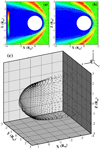 |
Fig. 1 Example of identified locations of the Martian MPB from simulation data on the X−Y plane (panel a), the X−Z plane (panel b), and in 3D (panel c) in the MSO coordinate system. The solar wind conditions for this example are BX = −1.6776 nT, BY = 2.4871 nT, BZ = 0 nT, and Pd = 1.06 nPa (n = 4.0 cm−3, VX = −400.0 km s−1 ). The black circles are the determined MPB locations in each panel. Panels a and b: color code displays the total pressure of solar wind (Ptot_sw = Pth_sw + Pd_sw in nPa) and the white arrows represent the vectors of the solar wind velocity. |
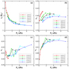 |
Fig. 2 Dependence of the MPB model parameters r0 (square in panel a), α0 (circle in panel b), α1 (gradient in panel c), and α2 (delta in panel d) on the solar wind dynamic pressure Pd corresponding to the different solar wind number density n. The IMF conditions are BX = −1.6776 nT, BY = 2.4871 nT, and BZ = 0 nT. The line segments connect adjacent points. The colors red, green, black, cyan, and blue represent n = 1, 3, 5, 7, and 9 cm−3, respectively. Further details of the simulations and fits are listed as cases 13–47 in the supplementary document. |
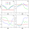 |
Fig. 3 Dependence of the MPB parameters r0 (square in panel a), α0 (circle in panel b), α1 (gradient in panel c), and α2 (delta in panel d) on the intensities of the IMF components BX (red), BY (blue), and BZ (green) for Pd = 1.06 nPa (n = 4.0 cm−3, VX = −400.0 km s−1). The IMF conditions were set with one component having a nonzero value, while the two other components were null. The line segments connect adjacent points. Further details concerning the case information are listed as cases 65–94 in the supplementary document. |
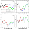 |
Fig. 4 IMF clock angle λ effects on the MPB parameters for BX = 0 nT (same format as in Fig. 3). The colors black, blue, green, and red represent λ varying with (1) Bt = 5 nT, BY < 0, Pd = 1.0 nPa, (2) Bt = 5 nT, BY > 0, Pd = 1.0 nPa, (3) Bt = 5 nT, BY > 0, Pd = 3.0 nPa, and (4) Bt = 10 nT, BY < 0, Pd = 5.0 nPa, respectively. Further details are listed in the supplementary document as cases 139–181. |
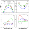 |
Fig. 5 Effects of the IMF cone angle µ on the MPB parameters (same format as in Fig. 3). The colors black, red, green, and blue correspond to the µ changed by varying BX for (1) Bt = 5 nT, BY < 0, BZ = 0, Pd = 1.0 nPa (cases 192–201), (2) Bt = 5 nT, BY > 0, BZ = 0, Pd = 1.0 nPa (cases 182–191), (3) Bt = 5 nT, BZ < 0, BY = 0, Pd = 1.0 nPa (cases 235–244), and (4) Bt = 5 nT, BZ > 0, BY = 0, Pd = 3.0 nPa (cases 245–254), respectively. |
 |
Fig. 6
|

 |
Fig. 7 Effects of the solar wind number density n and velocity V on the shape and size of the Martian MPB. |
 |
Fig. 8 Modeled effects of the IMF components BY, BZ, and the clock angle λ on the shape and size of the Martian MPB. |
4 Discussion
4.1 Mechanism of Solar Wind Effects on the Martian MPB
In general, a planetary magnetopause forms in the area where inside pressure approximately equals the outside pressure (e.g., Chapman & Ferraro 1931; Shue & Chao 2013; Lu et al. 2015). Although Mars is an unmagnetized planet, the inside pressure is mainly the magnetic pressure provided by the crustal fields (e.g., Holmberg et al. 2019). The outside pressure consists of the dynamic, thermal, and magnetic pressures (e.g., Brain et al. 2010; Wei et al. 2012; Holmberg et al. 2019; Zhang et al. 2019). As a result, when the upstream Pd increases, it pushes the MPB closer to the surface of Mars. In addition, the dayside region usually moves deeper than the flank region, and hence the flaring degree is enhanced with an increasing Pd (e.g., Shue et al. 1997). For a higher Pd when the MPB moves to a lower altitude and the asymmetry caused by the magnetic pileup process is expected to be more pronounced. Therefore, the dawn-dusk asymmetry increases with Pd. However, the north-south asymmetry caused by the intrinsic magnetic field is compensated by the stronger magnetic pileup process, and so it decreases with Pd.
The differences between the effects of the solar wind density and the velocity on the MPB can be explained by the magnetic pileup process. As the planetary ion pickup and solar wind mass loading processes are driven by the solar wind convection electric field (ESW = −VSW × BIMF), the IMF can pile up outside the ionosphere, in which the unmagnetized planet can prevent the penetration of the solar wind magnetic field by a diamagnetic current at the ionopause (e.g., Nagy et al. 2004; Fang et al. 2018). As a result, for a higher solar wind velocity under the same Pd, the solar wind convection electric field is higher for the same IMF conditions. The mass loading effect due to the pickup process also becomes stronger, which would cause a stronger magnetic pileup region (e.g., Modolo et al. 2006; Vaisberg et al. 2017; Chang et al. 2020). In this vein, for a higher solar wind velocity, the magnetic pressure at the Martian MPB should be higher (Wang et al. 2021). Moreover, at a higher magnetic field strength, the plasmas near the plasma depletion region (the inner part of the Martian magnetosheath where the magnetosheath magnetic fields are enhanced and the magnetosheath plasmas are partially depleted) are more easily squeezed out along the pileup magnetic field, which leads to a decrease in the plasma density, plasma β, and the ion temperature, especially for the hotter plasmas (e.g., Lee & Lee 2020; Wang et al. 2020b). Thus, the stronger magnetic pileup process for the higher solar wind velocity causes the magnetic pressure to increase and the thermal pressure to decrease at the Martian MPB. In addition, in the magnetosheath the thermal pressure dominates, while in the magnetosphere it is the magnetic pressure (Brain et al. 2010; Cui et al. 2018; Sánchez-Cano et al. 2020). As a result, for the same Pd, a higher solar wind velocity (a lower density) leads the MPB located farther away from Mars and having a higher flaring degree.
The mechanism by which the IMF affects the geometry of the Martian MPB is also due to the magnetic pileup process. As we mentioned above, the magnetic pileup process is caused by the interaction of the Martian ionosphere and the solar wind, in which the unmagnetized planet prevents the penetration of the solar wind magnetic field by the diamagnetic current at the ionopause, which results in the pileup of the IMF outside the ionosphere (e.g., Nagy et al. 2004; Fang et al. 2018). However, the IMF can only be compressed in the direction perpendicular to the solar wind speed, and hence only the IMF components perpendicular to the solar wind velocity, BY and BZ, participate in the process and determine the size of the pileup region (e.g., Wang et al. 2020a). The pileup process is stronger at a larger IMF intensity. As a result, larger BY and BZ result in a thicker pileup region and a farther MPB from Mars, which in turn increase the subsolar standoff distance and flaring degree of the MPB. For the IMF BX component, the IMF pileup is weak, so there is little effect of BX on the MPB. The IMF cone angle influence is also mainly due to the changing of the BY and BZ components. In addition, when the MPB moves away from Mars with increasing intensities of BY and BZ, the asymmetries of the MPB become smaller.
According to the classic magnetic field draping theory, at Mars the IMF is mainly piled up along the upstream IMF orientation in the plane perpendicular to the solar wind flow direction (e.g., Crider et al. 2004; Brain et al. 2005). Although these pileup and draping processes vary with the altitude and SZA (e.g., Fang et al. 2018), the IMF pileup is the strongest in the IMF clock angle direction (e.g., Luhmann et al. 2004). In this vein, however, the northward and southward BZ should have the same effect on the MPB, which disagrees with our model calculations. This disagreement, however, is explained by the magnetic field topology shown in Fig. 9.
Figure 9 shows the magnetic field topology in the X−Z plane for the northward and southward BZ. The intrinsic crustal magnetic field of Mars is complex and the intense crustal sources are mainly concentrated in the area of the southern hemisphere in the Terra Sirenum region, which is located in the longitude range 150° E to 240° E and the latitude range 30° S to 85° S (e.g., Acuna et al. 1999; Connerney et al. 1999). In this work, for nearly all of the simulations, the subsolar location was fixed to 180° W and 0° N, which means that the strongest crustal magnetic field was located on the dayside (Arkani-Hamed 2001; Ma et al. 2004). Panel a of Fig. 9 shows that for the northward BZ, the crustal field and the IMF are basically parallel at SZA ≈ 45°, which results in a thick pileup region. In contrast, for the southward BZ, shown in panel b, at SZA ≈ 45° the crustal fields and the IMF are antiparallel, causing magnetic reconnection and leading to the erosion of the crustal field (e.g., Brain et al. 2003). As a result, the MPB for southward IMF is located closer to the planet than for northward IMF. Meanwhile, the northern hemisphere of the MPB is not affected by this as the crustal field is relatively weak there, and its average location is in between the two conditions mentioned above. As a result, for the northward BZ, the MPB in the southern hemisphere is located farther away from the planet than the northern hemisphere and has a larger flaring degree. This also partly agrees with Edberg et al. (2009), who suggested that the southern hemisphere of the Martian MPB reacts differently to the IMF orientation than the northern hemisphere. As the absolute value of BZ increases, this north-south asymmetry decreases as the whole MPB moves away from Mars. Moreover, the effects of the IMF clock angle on the subsolar standoff distance and the flaring degree might also be associated with local magnetic reconnection, which needs further investigation in the future.
 |
Fig. 9 Magnetic field topology in the X−Z plane for BZ = 5 nT (panel a) and BZ = −5 nT (panel b). The solar wind conditions are IMF BX = BY = 0 nT, Pd = 1 nPa (n = 4.0 cm−3, VX = −400.0 km s−1 ). The color bar shows the solar wind total pressure (nPa) in each panel. The solid black lines are the magnetic field lines. The red circles and white squares represent the MPB location identified by the method in this work and the pressure balance (Pth + Pd)/PB = 1.0. The red dashed line is the model result of Vignes et al. (2000). |
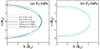 |
Fig. 10 Comparison of our parametric Martian MPB model with existing empirical models. Panels a and b: models for Pd = 1 nPa (n = 4.0 cm−3, VX = −400.0 km s−1) and Pd = 3 nPa (n = 7.186 cm−3, VX = −500.0 km s−1), respectively. The IMF conditions used for our model are the same for both panels: BX = −1.6776 nT, BY = 2.4871 nT, and BZ = 0 nT. Red dashed lines and green dashed lines represent our parametric model results in the X−Y and X−Z planes. Black, blue, and cyan solid lines show the results of Vignes et al. (2000), Edberg et al. (2008), and Ramstad et al. (2017), respectively. |
4.2 Model Comparison
In Fig. 10, we compare our parametric model of the Martian MPB to several existing empirical models for different solar wind conditions. It is worth mentioning that Vignes et al. (2000) and Edberg et al. (2008) models do not include any control parameters and only represent the MPB locations under the typical solar wind conditions in panel a.
Figure 10 shows that for Pd = 1 nPa (panel a), our parametric model is in agreement with the average location of the empirical models in the subsolar region, and is especially close to the Vignes et al. (2000) model. In the mid-latitude region, our model predicts the MPB being farther away from Mars than the other models, and in the tail region, our model also agrees with the empirical models well. For Pd = 3 nPa, the results are similar and the two models agree very well on the dayside. Our model is located a bit farther away from Mars in the mid-latitude region when compared to the model of Ramstad et al. (2017). The asymmetries of our model are summarized in Table 2.
The detailed comparison between the subsolar standoff distance r0 (RM) and the terminator distance LX=0 (RM) (measured from the Mars center) for different MPB models is presented in Table 2. For our parametric model, LX=0 values are displayed in the northern (ϕ = 0°), eastern (90°), southern (180°), and western (270°) directions. The IMF conditions used to calculate these values were the same as those used for Fig. 10. For Pd = 1 nPa, it appears that the Ramstad et al. (2017) model slightly underestimates the size of the Martian MPB (r0 = 1.218 RM), while our parametric model (r0 = 1.270 RM) is in closer agreement with the empirical models (1.29 and 1.33 RM). For Pd = 3 nPa, r0 = 1.190 RM for our parametric model is very close to the 1.187 RM of the Ramstad et al. (2017) model. Our model is the only one so far to include the asymmetries; the obvious asymmetries it shows are the in the north-south (Lϕ=180° > Lϕ=0° ) and dawn-dusk (Lϕ=90° > Lϕ=270°) directions. Asymmetries in the MPB location are expected and have been reported previously (e.g., Crider et al. 2002; Brain et al. 2003; Edberg et al. 2008, 2009; Fang et al. 2017; Matsunaga et al. 2017). In the future, the corresponding crossing data of the Martian MPB from multiple satellites, such as MGS, MEX, MAVEN, and Tianwen-1 can be used to validate and improve our model.
4.3 Effects of the Crustal Magnetic Field and the Solar Cycle
In this section, we make a first attempt at illustrating the effects of the orientation of the crustal magnetic fields and solar activity. We performed four simulations in which the subsolar positions of the crustal magnetic field were set to 180° W 0° N and 0° W 0° N, which represent the strong and weak crustal magnetic fields. For every orientation of the crustal field, we considered conditions typical for the maximum and minimum of the solar cycle (Ma et al. 2004). Table 3 shows the values of the model parameters r0, α0, α1, and α2 obtained directly from the simulation data, as well as the average terminator distance of the MPB from the Mars center at X = 0, Lx=0. The other solar wind conditions used for these four cases were Pd = 1 nPa (n = 4.0 cm−3, V = −400.0 km s−1), BX = −1.6776 nT, By = 2.4871 nT, and BZ = 0 nT.
Our results show that the MPB is located farther away from Mars under the solar maximum condition than under the solar minimum conditions, which agrees with Ramstad et al. (2017) and Lentz et al. (2021). Specifically, in the subsolar strong crustal field cases (180° W 0° N), Lx=0 and r0 were 3.793 and 0.7087% smaller, respectively, for solar minimum conditions than for solar maximum conditions. In weak crustal field cases (0° W 0° N), the differences were 6.246 and 6.544%, respectively. In both the solar maximum and minimum conditions, when the strong crustal field is located in the dayside region, the MPB moves away from Mars. Also, the flaring angle α0 is enhanced under the solar maximum condition, while it does not change too much under the solar minimum condition. Moreover, in solar maximum conditions, the southern hemisphere asymmetry is more prominent when the strong crustal field is located on the day-side, which agrees well with the results of Fang et al. (2017) and Matsunaga et al. (2017). In solar minimum conditions, the north-south asymmetry in the simulations is not obvious. In addition, our simulations also show that the effect of the crustal field on the MPB location is larger than that of the solar cycle. In the future, the effects of the crustal fields and the solar cycle need to be studied further and accounted for by Martian MPB models.
Comparison of our Martian MPB model with previous empirical models.
Preliminary effect of the crustal magnetic field (CM) and the solar cycle on the Martian magnetic pileup boundary.
5 Summary and Conclusions
Using a 3D multispecies MHD model, we constructed a 3D parametric Martian MPB model that includes the solar wind density and velocity, along with the intensity and orientation of the IMF, as controlling factors. We employed a modified parabola function to describe the shape and size of the Martian MPB. This shape function includes the north-south and dawn-dusk asymmetries, and is controlled by four model parameters. We determined the location of the MPB from the simulation data by combining the pressure balance and the flow speed gradient. A total of 267 individual simulations with different solar wind and IMF conditions were used to produce a database and calculate the four parameters of our MPB model. Conditions corresponding to the solar maximum and the strongest crustal field located on the day-side were used in most cases. Our main results are as follows: (1) the MPB moves close to Mars when the upstream Pd increases; the subsolar standoff distance decreases and the flaring degree of the Martian MPB increases with increasing Pd according to the power-law relations. Under the same Pd, a higher solar wind velocity (and, therefore, a lower density) leads to a farther location of the MPB from Mars and a larger flaring degree. This is explained by the higher solar wind convection electric field and the stronger magnetic pileup process under these conditions. (2) A larger IMF Y or Z component, BY or BZ, leads to a thicker pileup region and a farther MPB location from Mars, as well as a decrease in the flaring degree. There is little effect of the radial IMF component, BX, on the geometry of the MPB. (3) The conditions corresponding to the strongest crustal field located on the dayside were used in this work. Under these conditions, for the southward IMF, the Martian MPB is located farther away in the northern hemisphere than in the southern hemisphere, and this phenomenon is more prominent for a larger value of the southward IMF. While the well-known north-south asymmetry of the Martian MPB (the southern hemisphere of the MPB being farther away than the northern one) is only observed for other IMF directions. We suggest that the magnetic reconnection of the southward IMF and the crustal field that occurs at the middle latitude of the southern hemisphere results in the different magnetic field topologies and affects the location of the MPB.
The comparison shows a good agreement between our parametric model and the previous empirical models under typical solar wind conditions. There are two aspects of the model that should be improved in the future. First, several other factors, such as the location of the crustal magnetic fields (or the seasonal dependency) and the solar cycle (or solar EUV radiation) should be included. Second, the Martian MPB crossing from multiple satellites, such as MGS, MEX, MAVEN, and Tianwen-1 should be used to validate the model.
Acknowledgements
The work is supported by the National Natural Science Foundation of China (grant 42074195, 42030203, 41974190), Macau Foundation and the pre-research project on Civil Aerospace Technologies No. D020104, D020308 funded by China’s National Space Administration. This research is funded by Pandeng Program of National Space Science Center, Chinese Academy of Sciences. The work is also supported by the Specialized Research Fund for State Key Laboratories, Beijing Municipal Science and Technology Commission (Grant No. Z191100004319001), the Key Research Program of the Chinese Academy of Sciences, Grant No. ZDBS-SSW-TLC00103, and a grant from the “Macao Young Scholars Program” (Project code: AM201905). L. Xie was supported by the Youth Innovation Promotion Association of the Chinese Academy of Sciences. We acknowledge the CSEM team in University of Michigan for the use of BATS-R-US code. The numerical calculations in this paper have been carried out on the super computing system in the Super computing Center of Nanjing University of Information Science & Technology. We especially acknowledge Yingjuan Ma at UCLA for the multi-species MHD model used in this work.
References
- Acuna, M. H., Connerney, J. E. P., Ness, N. F., et al. 1999, Science, 284, 790 [NASA ADS] [CrossRef] [Google Scholar]
- Arkani-Hamed, J. 2001, J. Geophys. Res., 106, 23197 [Google Scholar]
- Bougher, S. W., Engel, S., Roble, R. G., et al. 2000, J. Geophys. Res., 105, 17669 [Google Scholar]
- Brain, D. A., Bagenal, F., Acuña, M. H., et al. 2003, J. Geophys. Res. Space Phys., 108, 1424 [NASA ADS] [Google Scholar]
- Brain, D. A., Halekas, J. S., Lillis, R., et al. 2005, Geophys. Res. Lett., 32, L18203 [Google Scholar]
- Brain, D., Barabash, S., Boesswetter, A., et al. 2010, Icarus, 206, 139 [Google Scholar]
- Chang, Q., Xu, X., Xu, Q., et al. 2020, ApJ, 900, 63 [Google Scholar]
- Chapman, S., & Ferraro, V. C. A. 1931, J. Geophys. Res., 36, 77 [Google Scholar]
- Connerney, J. E. P., Acuna, M. H., Wasilewski, P. J., et al. 1999, Science, 284, 794 [NASA ADS] [CrossRef] [Google Scholar]
- Crider, D. H., Acuña, M. H., Connerney, J. E. P., et al. 2002, Geophys. Res. Lett., 29, 1170 [Google Scholar]
- Crider, D. H., Vignes, D., Krymskii, A. M., et al. 2003, J. Geophys. Res. Space Phys., 108, 1461 [Google Scholar]
- Crider, D. H., Brain, D. A., Acuña, M. H., et al. 2004, Space Sci. Rev., 111, 203 [NASA ADS] [CrossRef] [Google Scholar]
- Cui, J., Yelle, R. V., Zhao, L.-L., et al. 2018, ApJ, 853, L33 [Google Scholar]
- DiBraccio, G. A., Luhmann, J. G., Curry, S. M., et al. 2018, Geophys. Res. Lett., 45, 4559 [NASA ADS] [CrossRef] [Google Scholar]
- Dong, C., Ma, Y., Bougher, S. W., et al. 2015, Geophys. Res. Lett., 42, 9103 [NASA ADS] [CrossRef] [Google Scholar]
- Dubinin, E., Fränz, M., Woch, J., et al. 2006, Space Sci. Rev., 126, 209 [CrossRef] [Google Scholar]
- Dubinin, E., Fränz, M., Woch, J., et al. 2007, The Mars Plasma Environment (Berlin: Springer), 209 [Google Scholar]
- Edberg, N. J. T., Lester, M., Cowley, S. W. H., et al. 2008, J. Geophys. Res. Space Phys., 113, A08206 [Google Scholar]
- Edberg, N. J. T., Brain, D. A., Lester, M., et al. 2009, Annal. Geophys., 27, 3537 [Google Scholar]
- Egan, H., Ma, Y., Dong, C., et al. 2018, J. Geophys. Res. Space Phys., 123, 3714 [NASA ADS] [Google Scholar]
- Fang, X., Liemohn, M. W., Nagy, A. F., et al. 2010, J. Geophys. Res. Space Phys., 115, A04308 [Google Scholar]
- Fang, X., Ma, Y., Brain, D., et al. 2015, J. Geophys. Res. Space Phys., 120, 10926 [NASA ADS] [Google Scholar]
- Fang, X., Ma, Y., Masunaga, K., et al. 2017, J. Geophys. Res. Space Phys., 122, 4117 [Google Scholar]
- Fang, X., Ma, Y., Luhmann, J., et al. 2018, Geophys. Res. Lett., 45, 3356 [Google Scholar]
- Halekas, J. S., Ruhunusiri, S., Harada, Y., et al. 2017, J. Geophys. Res. Space Phys., 122, 547 [NASA ADS] [CrossRef] [Google Scholar]
- Holmberg, M. K. G., André, N., Garnier, P., et al. 2019, J. Geophys. Res. Space Phys., 124, 8564 [Google Scholar]
- Jarvinen, R., Brain, D. A., Modolo, R., et al. 2018, J. Geophys. Res. Space Phys., 123, 1678 [NASA ADS] [Google Scholar]
- Kim, J., Nagy, A. F., Fox, J. L., et al. 1998, J. Geophys. Res., 103, 29339 [Google Scholar]
- Lee, L. C., & Lee, K. H. 2020, Rev. Mod. Plasma Phys., 4, 9 [Google Scholar]
- Lentz, C. L., Baker, D. N., Andersson, L., et al. 2021, J. Geophys. Res. Space Phys., 126, e28105 [NASA ADS] [Google Scholar]
- Lin, R. L., Zhang, X. X., Liu, S. Q., et al. 2010, J. Geophys. Res. Space Phys., 115, A04207 [Google Scholar]
- Liu, Z.-Q., Lu, J. Y., Wang, C., et al. 2015, J. Geophys. Res. Space Phys., 120, 5645 [Google Scholar]
- Liu, D., Rong, Z., Gao, J., et al. 2021, ApJ, 911, 113 [NASA ADS] [CrossRef] [Google Scholar]
- Lu, J. Y., Liu, Z.-Q., Kabin, K., et al. 2011, J. Geophys. Res. Space Phys., 116, A09237 [Google Scholar]
- Lu, J. Y., Wang, M., Kabin, K., et al. 2015, Planet. Space Sci., 106, 108 [Google Scholar]
- Luhmann, J. G., Ledvina, S. A., & Russell, C. T. 2004, Adv. Space Res., 33, 1905 [Google Scholar]
- Lundin, R., Barabash, S., Andersson, H., et al. 2004, Science, 305, 1933 [NASA ADS] [CrossRef] [Google Scholar]
- Lundin, R., Barabash, S., Holmström, M., et al. 2013, Geophys. Res. Lett., 40, 6028 [Google Scholar]
- Ma, Y., Nagy, A. F., Sokolov, I. V., et al. 2004, J. Geophys. Res. Space Phys., 109, A07211 [Google Scholar]
- Ma, Y., Russell, C. T., Nagy, A. F., et al. 2013, AGU Fall Meeting Abstracts, P13C-05 [Google Scholar]
- Ma, Y. J., Fang, X., Nagy, A. F., et al. 2014a, J. Geophys. Res. Space Phys., 119, 1272 [Google Scholar]
- Ma, Y., Fang, X., Russell, C. T., et al. 2014b, Geophys. Res. Lett., 41, 6563 [Google Scholar]
- Matsunaga, K., Seki, K., Hara, T., et al. 2015, J. Geophys. Res. Space Phys., 120, 6874. [Google Scholar]
- Matsunaga, K., Seki, K., Brain, D. A., et al. 2017, J. Geophys. Res. Space Phys., 122, 9723 [Google Scholar]
- Modolo, R., Chanteur, G. M., Dubinin, E., et al. 2006, Ann. Geophys., 24, 3403 [NASA ADS] [CrossRef] [Google Scholar]
- Modolo, R., Hess, S., Mancini, M., et al. 2016, J. Geophys. Res. Space Phys., 121, 6378 [NASA ADS] [Google Scholar]
- Nagy, A. F., Winterhalter, D., Sauer, K., et al. 2004, Space Sci. Rev., 111, 33 [NASA ADS] [CrossRef] [Google Scholar]
- Najib, D., Nagy, A. F., Tóth, G., et al. 2011, J. Geophys. Rese. Space Phys., 116, A05204 [NASA ADS] [Google Scholar]
- Němec, F., Linzmayer, V., Nemecek, Z., et al. 2020, J. Geophys. Res. Space Phys., 125, e28509 [Google Scholar]
- Ramstad, R., Barabash, S., Futaana, Y., et al. 2017, J. Geophys. Rese. Space Phys., 122, 7279 [NASA ADS] [CrossRef] [Google Scholar]
- Samsonov, A. A., Bogdanova, Y. V., Branduardi-Raymont, G., et al. 2020, Geophys. Res. Lett., 47, e86474 [Google Scholar]
- Sánchez-Cano, B., Narvaez, C., Lester, M., et al. 2020, J. Geophys. Res. Space Phys., 125, e28145 [Google Scholar]
- Shue, J.-H., & Chao, J.-K. 2013, J. Geophys. Res. Space Phys., 118, 3017 [Google Scholar]
- Shue, J.-H., Chao, J. K., Fu, H. C., et al. 1997, J. Geophys. Res., 102, 9497 [Google Scholar]
- Tóth, G., van der Holst, B., Sokolov, I. V., et al. 2012, J. Comput. Phys., 231, 870 [Google Scholar]
- Trotignon, J. G., Mazelle, C., Bertucci, C., et al. 2006, Planet. Space Sci., 54, 357 [Google Scholar]
- Vaisberg, O. L., Ermakov, V. N., Shuvalov, S. D., et al. 2017, Planet. Space Sci., 147, 28 [Google Scholar]
- Verigin, M. I., Gringauz, K. I., Kotova, G. A., et al. 1993, J. Geophys. Res., 98, 1303 [Google Scholar]
- Vignes, D., Mazelle, C., Rme, H., et al. 2000, Geophys. Res. Lett., 27, 49 [Google Scholar]
- Wang, M., Xie, L., Lee, L. C., et al. 2020a, ApJ, 903, 125 [Google Scholar]
- Wang, J., Lee, L. C., Xu, X., et al. 2020b, A&A, 642, A34 [NASA ADS] [CrossRef] [EDP Sciences] [Google Scholar]
- Wang, M., Lee, L. C., Xie, L., et al. 2021, A&A, 651, A22 [NASA ADS] [CrossRef] [EDP Sciences] [Google Scholar]
- Weber, T., Brain, D., Xu, S., et al. 2020, Geophys. Res. Lett., 47, e87757 [NASA ADS] [Google Scholar]
- Wei, Y., Fraenz, M., Dubinin, E., et al. 2012, J. Geophys. Res. Space Physics, 117, A03208 [NASA ADS] [Google Scholar]
- Xu, S., Liemohn, M. W., Dong, C., et al. 2016, J. Geophys. Res. Space Phys., 121, 6417 [NASA ADS] [CrossRef] [Google Scholar]
- Xu, S., Mitchell, D. L., Weber, T., et al. 2020, J. Geophys. Res. Space Physics, 125, e27755 [NASA ADS] [Google Scholar]
- Zhang, H., Fu, S., Pu, Z., et al. 2019, ApJ, 880, 122 [NASA ADS] [CrossRef] [Google Scholar]
All Tables
Preliminary effect of the crustal magnetic field (CM) and the solar cycle on the Martian magnetic pileup boundary.
All Figures
|
Fig. 1 Example of identified locations of the Martian MPB from simulation data on the X−Y plane (panel a), the X−Z plane (panel b), and in 3D (panel c) in the MSO coordinate system. The solar wind conditions for this example are BX = −1.6776 nT, BY = 2.4871 nT, BZ = 0 nT, and Pd = 1.06 nPa (n = 4.0 cm−3, VX = −400.0 km s−1 ). The black circles are the determined MPB locations in each panel. Panels a and b: color code displays the total pressure of solar wind (Ptot_sw = Pth_sw + Pd_sw in nPa) and the white arrows represent the vectors of the solar wind velocity. |
| In the text | |
|
Fig. 2 Dependence of the MPB model parameters r0 (square in panel a), α0 (circle in panel b), α1 (gradient in panel c), and α2 (delta in panel d) on the solar wind dynamic pressure Pd corresponding to the different solar wind number density n. The IMF conditions are BX = −1.6776 nT, BY = 2.4871 nT, and BZ = 0 nT. The line segments connect adjacent points. The colors red, green, black, cyan, and blue represent n = 1, 3, 5, 7, and 9 cm−3, respectively. Further details of the simulations and fits are listed as cases 13–47 in the supplementary document. |
| In the text | |
|
Fig. 3 Dependence of the MPB parameters r0 (square in panel a), α0 (circle in panel b), α1 (gradient in panel c), and α2 (delta in panel d) on the intensities of the IMF components BX (red), BY (blue), and BZ (green) for Pd = 1.06 nPa (n = 4.0 cm−3, VX = −400.0 km s−1). The IMF conditions were set with one component having a nonzero value, while the two other components were null. The line segments connect adjacent points. Further details concerning the case information are listed as cases 65–94 in the supplementary document. |
| In the text | |
|
Fig. 4 IMF clock angle λ effects on the MPB parameters for BX = 0 nT (same format as in Fig. 3). The colors black, blue, green, and red represent λ varying with (1) Bt = 5 nT, BY < 0, Pd = 1.0 nPa, (2) Bt = 5 nT, BY > 0, Pd = 1.0 nPa, (3) Bt = 5 nT, BY > 0, Pd = 3.0 nPa, and (4) Bt = 10 nT, BY < 0, Pd = 5.0 nPa, respectively. Further details are listed in the supplementary document as cases 139–181. |
| In the text | |
|
Fig. 5 Effects of the IMF cone angle µ on the MPB parameters (same format as in Fig. 3). The colors black, red, green, and blue correspond to the µ changed by varying BX for (1) Bt = 5 nT, BY < 0, BZ = 0, Pd = 1.0 nPa (cases 192–201), (2) Bt = 5 nT, BY > 0, BZ = 0, Pd = 1.0 nPa (cases 182–191), (3) Bt = 5 nT, BZ < 0, BY = 0, Pd = 1.0 nPa (cases 235–244), and (4) Bt = 5 nT, BZ > 0, BY = 0, Pd = 3.0 nPa (cases 245–254), respectively. |
| In the text | |
|
Fig. 6
|
| In the text | |
|
Fig. 7 Effects of the solar wind number density n and velocity V on the shape and size of the Martian MPB. |
| In the text | |
|
Fig. 8 Modeled effects of the IMF components BY, BZ, and the clock angle λ on the shape and size of the Martian MPB. |
| In the text | |
|
Fig. 9 Magnetic field topology in the X−Z plane for BZ = 5 nT (panel a) and BZ = −5 nT (panel b). The solar wind conditions are IMF BX = BY = 0 nT, Pd = 1 nPa (n = 4.0 cm−3, VX = −400.0 km s−1 ). The color bar shows the solar wind total pressure (nPa) in each panel. The solid black lines are the magnetic field lines. The red circles and white squares represent the MPB location identified by the method in this work and the pressure balance (Pth + Pd)/PB = 1.0. The red dashed line is the model result of Vignes et al. (2000). |
| In the text | |
|
Fig. 10 Comparison of our parametric Martian MPB model with existing empirical models. Panels a and b: models for Pd = 1 nPa (n = 4.0 cm−3, VX = −400.0 km s−1) and Pd = 3 nPa (n = 7.186 cm−3, VX = −500.0 km s−1), respectively. The IMF conditions used for our model are the same for both panels: BX = −1.6776 nT, BY = 2.4871 nT, and BZ = 0 nT. Red dashed lines and green dashed lines represent our parametric model results in the X−Y and X−Z planes. Black, blue, and cyan solid lines show the results of Vignes et al. (2000), Edberg et al. (2008), and Ramstad et al. (2017), respectively. |
| In the text | |
Current usage metrics show cumulative count of Article Views (full-text article views including HTML views, PDF and ePub downloads, according to the available data) and Abstracts Views on Vision4Press platform.
Data correspond to usage on the plateform after 2015. The current usage metrics is available 48-96 hours after online publication and is updated daily on week days.
Initial download of the metrics may take a while.