| Issue |
A&A
Volume 697, May 2025
|
|
|---|---|---|
| Article Number | A113 | |
| Number of page(s) | 6 | |
| Section | Planets, planetary systems, and small bodies | |
| DOI | https://doi.org/10.1051/0004-6361/202452882 | |
| Published online | 12 May 2025 | |
The nature of Martian plume during solar wind interaction with Mars
1
School of Space and Earth Science, Beihang University,
Beijing,
China
2
Key Laboratory of Space Environment Monitoring and Information Processing, Ministry of Industry and Information Technology,
Beijing,
China
★ Corresponding author: This email address is being protected from spambots. You need JavaScript enabled to view it.
Received:
5
November
2024
Accepted:
25
March
2025
Abstract
Investigating the physical mechanism of ion escape on Mars is crucial for comprehending the evolution of Martian space environment. The plume structure located in the +E hemisphere of Mars plays a crucial role in the escape of planetary ions, contributing more than 20 percent to the overall ion escape rate. In this study, a three-dimensional multi-fluid Hall magnetohydrodynamics (MHD) numerical model is utilized to simulate the ion escape process of Mars. A force analysis is conducted to examine the electric field exerted on O+ and to investigate the density, velocity, and escape flux of O+. Numerical results indicate that both the convection field and the magnetic force field play essential roles in driving ion escape in the plume region and shaping the morphology of ion escaping fluxes. The plume is positioned above the magnetic pile-up boundary (MPB), as the convection field directed towards the +Z direction primarily influences the area above the MPB. Furthermore, the Hall field points outward and reaches the peak values at the MPB, while the ambipolar field peaks at the bow shock (BS). In addition, the ions escaping from the plume predominantly originates from the middle and high latitudes of the +E hemisphere on the Martian dayside. The plume escape rate and the tail escape rate are 4.33 × 10²³ s−1 and 1.74 × 1024 s−1 respectively. The plume escape rate accounts for 24.83% of the tail escape rate and 19.89% of the overall escape rate.
Key words: magnetohydrodynamics (MHD) / methods: numerical / planets and satellites: terrestrial planets
© The Authors 2025
 Open Access article, published by EDP Sciences, under the terms of the Creative Commons Attribution License (https://creativecommons.org/licenses/by/4.0), which permits unrestricted use, distribution, and reproduction in any medium, provided the original work is properly cited.
This article is published in open access under the Subscribe to Open model. This email address is being protected from spambots. You need JavaScript enabled to view it. to support open access publication.
1 Introduction
In recent years, Mars has attracted significant attention in planetary science research, due to its potential as a habitable planet. Unlike Earth, which is warm and moist, Mars is currently characterized by cold and dry conditions. However, numerous pieces of evidence indicate the existence of liquid water on the ancient surface of Mars. The hypothesis that Mars once possessed water is supported by the data of NASA’s Spirit rover, which uncovered hydrated minerals with crystal structures that imply the existence of liquid water (e.g., Johnson 2018; Orosei et al. 2018). It is widely believed that the change in Mars’ conditions can be influenced by its plasma environment and the subsequent loss of atmospheric ions. Unlike Earth, Mars lacks a dipole magnetic field and instead possesses a localized and unevenly distributed crustal magnetic field primarily concentrated in the southern hemisphere, which complicates the interaction between the solar wind and Mars.
Although the induced magnetosphere of the unmagnetized planets provides some protection from sputtering and ion pickup, Mars’ upper atmosphere interacts directly with the solar wind, due to the absence of a global dipole magnetic field similar to Earth’s (e.g., Gunell et al. 2018). Solar radiation leads to the formation of the ionosphere, which is primarily composed of ![Mathematical equation: $\[\mathrm{O}_2^{+}\]$](/articles/aa/full_html/2025/05/aa52882-24/aa52882-24-eq1.png) , O+, and
, O+, and ![Mathematical equation: $\[\mathrm{CO}_{2}^{+}\]$](/articles/aa/full_html/2025/05/aa52882-24/aa52882-24-eq2.png) ions produced through various chemical reactions such as photoionization and charge exchange. The Martian ionosphere and the crustal magnetic field are able to resist the incoming solar wind plasma. The bow shock is generated by the interaction of the supersonic solar wind flow, while the magnetic pileup results from mass loading effects. The heavy planetary ions are lost during the process of ion escape, which can be categorized into two main types based on the distinct locations of the escape channels: tailward escape and plume escape. It has been estimated that ion escape through the plume constitutes approximately 30% of the tail escape rate and 23% of the overall escape rate (e.g., Dong et al. 2015).
ions produced through various chemical reactions such as photoionization and charge exchange. The Martian ionosphere and the crustal magnetic field are able to resist the incoming solar wind plasma. The bow shock is generated by the interaction of the supersonic solar wind flow, while the magnetic pileup results from mass loading effects. The heavy planetary ions are lost during the process of ion escape, which can be categorized into two main types based on the distinct locations of the escape channels: tailward escape and plume escape. It has been estimated that ion escape through the plume constitutes approximately 30% of the tail escape rate and 23% of the overall escape rate (e.g., Dong et al. 2015).
The plume structure in the +E hemisphere of Mars is notable for its unique and stable plasma configuration, where in the convection the electric field points away from the planet +Esw (e.g., Fang et al. 2008; Najib et al. 2011; Hinton et al. 2024). The convection electric field is able to accelerate heavy planetary ions to higher altitudes in a direction perpendicular to the solar wind flow rather than being deflected by the magnetic field and gravity. The movement of these ions is constrained within a range of angles spanning from +Esw to the tailward direction. In addition, the gyroradius of these ions corresponds to a few times the radius of Mars (e.g., Jarvinen et al. 2016). Consequently, their trajectory may extend well beyond the bow shock (BS) before their cycloid motion bends them in the direction of the solar wind. As the solar wind crosses the BS, it undergoes significant deceleration, accompanied by the accumulation and strengthening of magnetic field, leading to a discrepancy between two distinct regions within the plume structure (e.g., Fang et al. 2008).
While previous studies have indicated that the characteristics of the plume structure are governed by the convection electric field, it has been demonstrated that the electric field in the Martian space environment is highly intricate (e.g., Li et al. 2022, 2023; Song et al. 2023). The convection electric field is dominant downstream of the BS and the magnetosheath along the ZMS E direction. The Hall electric field is also crucial in the magnetic pileup boundary (MPB), while the ambipolar electric field makes important contributions in the BS. It is necessary to investigate the roles played by various electric field components, including convection, Hall, and ambipolar electric fields, in the shaping the plume structure. For this study we employed the three-dimensional multi-fluid model for the Martian space environment, which incorporates the Hall effect, to investigate the mechanism behind plume formation. The structure of the paper is as follows. Section 2 provides detailed descriptions of the model and simulation runs. Section 3 presents the findings and discusses the results of these simulations. Finally, Section 4 summarizes our conclusions and key findings.
2 Model description
The numerical model employed for this paper is a threedimensional multi-fluid magnetohydrodynamics (MHD) model, which includes the Navier-Stokes equations of four primary ion species present in the Martian ionosphere: H+, ![Mathematical equation: $\[\mathrm{O}_{2}^{+}\]$](/articles/aa/full_html/2025/05/aa52882-24/aa52882-24-eq3.png) , O+, and
, O+, and ![Mathematical equation: $\[\mathrm{CO}_{2}^{+}\]$](/articles/aa/full_html/2025/05/aa52882-24/aa52882-24-eq4.png) (e.g., Li et al. 2021). These ions are self-consistently generated by the three major chemical reactions occurring in the ionosphere: photoionization, charge exchange, and recombination reactions (e.g., Ma et al. 2004; Najib et al. 2011). Additionally, the model incorporates the Chapman function to calculate the photoionization rates, facilitating a more accurate simulation of the M2 layer of Mars.
(e.g., Li et al. 2021). These ions are self-consistently generated by the three major chemical reactions occurring in the ionosphere: photoionization, charge exchange, and recombination reactions (e.g., Ma et al. 2004; Najib et al. 2011). Additionally, the model incorporates the Chapman function to calculate the photoionization rates, facilitating a more accurate simulation of the M2 layer of Mars.
The governing equations for each ion component “s” are composed of the continuity equation, the momentum equation, and the energy conservation equation, which can be expressed as follows (e.g., Li et al. 2022, 2023; Najib et al. 2011):
![Mathematical equation: $\[\frac{\partial \rho_s}{\partial t}+\nabla \bullet\left(\rho_s \boldsymbol{u}_s\right)=\frac{\delta \rho_s}{\delta t},\]$](/articles/aa/full_html/2025/05/aa52882-24/aa52882-24-eq5.png) (1)
(1)
![Mathematical equation: $\[\begin{aligned}& \frac{\partial\left(\rho_s \boldsymbol{u}_s\right)}{\partial t}+\nabla \bullet\left(\rho_s \boldsymbol{u}_s \boldsymbol{u}_s+\boldsymbol{I} p_s\right) \\& =n_s q_s\left(\boldsymbol{u}_s-\boldsymbol{u}_{+}\right) \times \boldsymbol{B}+\frac{n_s ~q_s}{n_e ~e}\left(\boldsymbol{J} \times \boldsymbol{B}-\nabla p_e\right)+\frac{\delta M_s}{\delta t},\end{aligned}\]$](/articles/aa/full_html/2025/05/aa52882-24/aa52882-24-eq6.png) (2)
(2)
![Mathematical equation: $\[\begin{aligned}& \frac{\partial e_s}{\partial t}+\nabla \bullet\left[\left(e_s+p_s\right) \boldsymbol{u}_s\right] \\& =\boldsymbol{u}_s \bullet\left[\frac{n_s ~q_s}{n_e ~e}\left(\boldsymbol{J} \times \boldsymbol{B}-\nabla p_e\right)+n_s ~q_s\left(\boldsymbol{u}_s-\boldsymbol{u}_{+}\right) \times \boldsymbol{B}\right]+\frac{\delta E_s}{\delta t},\end{aligned}\]$](/articles/aa/full_html/2025/05/aa52882-24/aa52882-24-eq7.png) (3)
(3)
where, ![Mathematical equation: $\[e_{s}=\frac{1}{2} \rho_{s} \boldsymbol{u}_{s}^{2}+\frac{p_{s}}{\gamma-1}, \rho_{s}, \boldsymbol{u}_{s}, p_{s}, n_{s}\]$](/articles/aa/full_html/2025/05/aa52882-24/aa52882-24-eq8.png) , and qs respectively represent the energy density, mass density, velocity, ion pressure, number density, and charge of the ions. Here γ represents the ratio of specific heat (taken as 5/3 in this paper). B stands for the magnetic field, and J denotes the current density. pe and ne represent the electron pressure and electron number density, respectively. Following the quasi-neutrality assumption of the plasma, the electron number density ne = ∑i=ions ni. In addition, we assume that the electron pressure pe = ∑i=ions pi.
, and qs respectively represent the energy density, mass density, velocity, ion pressure, number density, and charge of the ions. Here γ represents the ratio of specific heat (taken as 5/3 in this paper). B stands for the magnetic field, and J denotes the current density. pe and ne represent the electron pressure and electron number density, respectively. Following the quasi-neutrality assumption of the plasma, the electron number density ne = ∑i=ions ni. In addition, we assume that the electron pressure pe = ∑i=ions pi.
The source terms, ![Mathematical equation: $\[\frac{\partial \rho_{s}}{\partial t}, \frac{\delta M_{s}}{\delta t}, \frac{\delta E_{s}}{\delta t}\]$](/articles/aa/full_html/2025/05/aa52882-24/aa52882-24-eq9.png) in Equations (1)–(3) respectively denote the changes in mass density, momentum, and energy for each species resulting from chemical reactions, including charge exchange, photoionization, and recombination among individual ion components. These source terms can be written as
in Equations (1)–(3) respectively denote the changes in mass density, momentum, and energy for each species resulting from chemical reactions, including charge exchange, photoionization, and recombination among individual ion components. These source terms can be written as
![Mathematical equation: $\[\frac{\delta \rho_s}{\delta t}=\boldsymbol{S}_s-\boldsymbol{L}_s,\]$](/articles/aa/full_html/2025/05/aa52882-24/aa52882-24-eq10.png) (4)
(4)
![Mathematical equation: $\[\frac{\delta \boldsymbol{M}_s}{\delta t}=\rho_s \sum_{t=neutral } \boldsymbol{v}_{s t}\left(\boldsymbol{u}_n-\boldsymbol{u}_s\right)+\boldsymbol{S}_s u_n-\boldsymbol{L}_s u_s,\]$](/articles/aa/full_html/2025/05/aa52882-24/aa52882-24-eq11.png) (5)
(5)
![Mathematical equation: $\[\begin{aligned}\frac{\delta \boldsymbol{E}_s}{\delta t}= & \sum_{t=\text { neutral }} \frac{\rho_s v_{s t}}{m_s+m_t}\left[3 \kappa\left(\boldsymbol{T}_n-\boldsymbol{T}_s\right)+m_t\left(\boldsymbol{u}_n-\boldsymbol{u}_s\right)^2\right] \\& +\frac{\kappa}{\gamma-1} \cdot \frac{\boldsymbol{S}_s \boldsymbol{T}_n-\boldsymbol{L}_s \boldsymbol{T}_s}{m_s}+\frac{1}{2}\left(\boldsymbol{S}_s \boldsymbol{u}_n^2-\boldsymbol{L}_s \boldsymbol{u}_s^2\right) \\& +\frac{n_s}{n_e} \cdot \frac{\kappa}{\gamma-1} \cdot \frac{\boldsymbol{S}_e \boldsymbol{T}_n-\boldsymbol{L}_s \boldsymbol{T}_s}{m_e},\end{aligned}\]$](/articles/aa/full_html/2025/05/aa52882-24/aa52882-24-eq12.png) (6)
(6)
where Ss and Ls respectively represent the production and loss rates of ionic species s; vst denotes the collision frequency between species s and t; un and Tn respectively represent the velocity and temperature of the neutral species “n”; Tn and ms respectively represent the temperature and mass of the ionic species “s”; and κ represents the Boltzmann constant.
Introducing the parameter charge-averaged ion velocity ![Mathematical equation: $\[\boldsymbol{u}_{+}=\frac{1}{e n_{e}} \sum_{s} n_{s} q_{s} \boldsymbol{u}_{s}\]$](/articles/aa/full_html/2025/05/aa52882-24/aa52882-24-eq13.png) and the electron velocity
and the electron velocity ![Mathematical equation: $\[\boldsymbol{u}_{e}=\boldsymbol{u}_{+}-\frac{1}{e n_{e}}\]$](/articles/aa/full_html/2025/05/aa52882-24/aa52882-24-eq14.png) , the magnetic induction equation is expressed as follows:
, the magnetic induction equation is expressed as follows:
![Mathematical equation: $\[\frac{\partial \boldsymbol{B}}{\partial t}-\nabla \times\left(\boldsymbol{u}_{+} \times \boldsymbol{B}-\frac{\boldsymbol{J} \times \boldsymbol{B}}{e n_e}+\frac{\nabla P_e}{e n_e}\right)=0.\]$](/articles/aa/full_html/2025/05/aa52882-24/aa52882-24-eq15.png) (7)
(7)
The model adopts the Mars-centered Solar Orbital (MSO) coordinate system, where the X-axis points from Mars toward the Sun, the Z-axis is perpendicular to the X-axis and points toward the Martian north ecliptic pole, and the Y-axis completes the right-hand coordinate system. In comparison to the Mars-Sun-Electric (MSE) coordinate system used in previous studies, the northern hemisphere (MSO) corresponds to the same region as the +E hemisphere (MSE). The computational domain is defined within the region of −24RM ≤ X ≤ 8RM, −16RM ≤ Y, Z ≤ 16RM, where RM is the radius of Mars (RV ≈ 3396 km). The inner boundary is set to be 100 km above the Martian surface, where the ion density at the inner boundary is assumed as the value of photochemical equilibrium. The model grid consists of 56 blocks and 100 × 120 × 80 = 960 000 computational cells, with the smallest grid size set to be 10 km. At the inner boundary of the lowest layer, the velocity and density of H+ are set to 0 and 0.3 times the solar wind density, respectively (e.g., Dong et al. 2015). The neutral density profile derived from Bougher (e.g., Bougher et al. 2000) is adopted as the initial value, facilitating a better comparison of differences between the northern and southern hemispheres of Mars.
A typical event with solar wind parameters in quiet-time conditions is set as follows: nsw = 2 cm−3, |Usw| = 566 km/s, |BIMF| = 3nT, and T = 3.5 × 10⁵ K (e.g., Liu et al. 2021). This event was chosen to demonstrate a characteristic plasma distribution under average conditions. Assuming that the solar wind follows a Parker spiral mode, an angle of 56° in the MSO coordinate system was selected and represented as (BX, BY, BZ) = (−1.6, 2.5, 0)nT. The subsolar point is positioned at 180° longitude on the equatorial plane. The G110 Martian crustal magnetic field model proposed by (e.g., Gao et al. 2021), was adopted in our simulation.
The electric field plays a crucial role in controlling ion transport and its characteristics, which ultimately determine whether the pickup ions escape tailward or escape through the plume (e.g., Fang et al. 2010). Benefiting from the involvement of ionkinetic scaled generalized Ohm’s law in our multi-fluid MHD model, it is anticipated that the nature and source of the Martian plume structure during the process of solar wind interaction with Mars would be well revealed through force analysis.
The equation of motion for charged particles can be written as
![Mathematical equation: $\[\boldsymbol{F}_s=n_s q_s\left(\boldsymbol{E}+\boldsymbol{u}_s \times \boldsymbol{B}\right),\]$](/articles/aa/full_html/2025/05/aa52882-24/aa52882-24-eq16.png) (8)
(8)
where the electric field force (nsqsE) governs both the acceleration and deflection of ions, while the magnetic force (nsqsus × B) mainly functions to deflect the ions. On the ion kinetic scale, the electric field consists of three components: the convection field, the Hall field, and the ambipolar field, which can be expressed as follows (the convection field, the Hall field, and the ambipolar field are all electric fields):
![Mathematical equation: $\[\boldsymbol{E}=-\boldsymbol{u}_{+} \times \boldsymbol{B}+\frac{\boldsymbol{J} \times \boldsymbol{B}}{e n_e}-\frac{\nabla P_e}{e n_e}.\]$](/articles/aa/full_html/2025/05/aa52882-24/aa52882-24-eq17.png) (9)
(9)
Here u+ represents the charge-averaged ion velocity (![Mathematical equation: $\[\boldsymbol{u}_{+}=\frac{1}{e n_{e}} \sum_{s} n_{s} q_{s} \boldsymbol{u}_{s}\]$](/articles/aa/full_html/2025/05/aa52882-24/aa52882-24-eq18.png) ), while us denotes the single-species ion velocity (specifically O+ in this paper).
), while us denotes the single-species ion velocity (specifically O+ in this paper).
When comparing Equations (8) and (9), it becomes evident that the term us × B significantly influences the total electromagnetic field. Hence, we designate us × B as the field of magnetic force in order to draw parallels with the components of the electric field.
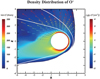 |
Fig. 1 Density and velocity of O+ ions in the X − Z Plane. The color plot represents ion density; the areas where the oxygen ion density is less than 0.001cm−3 have been blanked out. The white lines represent the magnetic pileup boundary (MPB, internally) and the bow shock (BS, externally) according to the empirical model by Vignes et al. (2000). The arrows depict the velocity vectors of O+ ions. |
3 Simulation results and analysis
3.1 Physical process behind the formation of plume structures
Figure 1 illustrates the spatial distribution of O+ density and velocity within the X − Z plane. For clarity, the areas where the oxygen ion density is less than 0.001 cm−3 have been blanked out. The locations of the MPB and BS predicted by the empirical model are superimposed on the color plots. The distribution of ion density and velocity shows a pronounced north-south asymmetry, with a prominent plume structure forming in the northern hemisphere, consistent with previous studies (e.g., Jarvinen et al. 2018; Najib et al. 2011; Fang et al. 2015).
In addition, the plume structure is intersected by boundary layers, such as the BS and MPB, motivating us to define two distinct parts of the plume structure. One part is termed the downstream plume, which encompasses the portion with altitudes lower than the BS, while the upstream plume comprises the remaining portion. As depicted in Figure 1, the O+ velocity in the downstream plume points to the −X and +Z directions, while in the upstream plume the velocity primarily aligns along the +Z direction. The density of O+ at ionospheric altitude shows a noticeable north-south asymmetry. The ionosphere in the southern hemisphere appears more expanded compared to that of the north, which can be attributed to the prominent effect of the strong crustal magnetic fields on the Martian ionosphere.
The advantage of our three-dimensional multi-fluid Hall MHD model lies in its ability to show the physical mechanism underlying the formation of the plume. As indicated by the momentum equations in Equation (2), the electromagnetic (EM) field includes the convection field (−u+ × B), the Hall field ![Mathematical equation: $\[\left(\frac{J \times \boldsymbol{B}}{e n_{e}}\right)\]$](/articles/aa/full_html/2025/05/aa52882-24/aa52882-24-eq19.png) , the ambipolar field
, the ambipolar field ![Mathematical equation: $\[\left(\frac{\nabla P_{e}}{e n_{e}}\right)\]$](/articles/aa/full_html/2025/05/aa52882-24/aa52882-24-eq20.png) , and the field of magnetic force (us × B). We emphasize that the magnetic force plays a crucial role in deflecting pickup ions, thus altering the trajectories, but it does not influence the acceleration process of these ions. This process is important for understanding the motion of pickup ions in the magnetic field.
, and the field of magnetic force (us × B). We emphasize that the magnetic force plays a crucial role in deflecting pickup ions, thus altering the trajectories, but it does not influence the acceleration process of these ions. This process is important for understanding the motion of pickup ions in the magnetic field.
To depict the morphology of the EM field while showing its asymmetry features, Figure 2 presents each component of the EM field in the X − Z plane, alongside the total field. The simulation results indicate that the magnitude of the total field is much stronger in the downstream plume than in the upstream plume; the maximum values are located at the MPB and BS. In both plume regions, the direction of the total field in the X − Z plane is almost parallel, pointing to the −X + Z direction, which is consistent with previous observations and simulations (e.g., Najib et al. 2011; Fang et al. 2015; Jarvinen et al. 2018; Ma et al. 2019). It can be seen from Figure 2b that the convection field (−u+ × B) reaches its maximum at both the BS and MPB. Moreover, its intensity is more pronounced in the downstream plume, which can be attributed to the magnetic field’s accumulation (e.g., Ma et al. 2019). The vectors of the convection field in the downstream plume direct away from Mars toward the MPB, while in the upstream plume regions it predominantly aligns with the +Z direction. In addition, the convection field within the plume is perpendicular to the MPB. Figures 2c and 2d show the Hall field ![Mathematical equation: $\[\left(\frac{J {\times} \boldsymbol{B}}{e n_{e}}\right)\]$](/articles/aa/full_html/2025/05/aa52882-24/aa52882-24-eq21.png) and ambipolar field
and ambipolar field ![Mathematical equation: $\[\left(\frac{\nabla P_{e}}{e n_{e}}\right)\]$](/articles/aa/full_html/2025/05/aa52882-24/aa52882-24-eq22.png) , respectively, which indicate that the Hall and ambipolar fields are both primarily concentrated near the MPB and BS, peaking outward to decelerate solar wind plasma. The ambipolar field reaches its peak intensity near the subsolar region and decreases as the solar zenith angle (SZA) increases, which is consistent with recent statistical results (e.g., Xu et al. 2021). In addition, Figure 2e displays a color plot and vectors of the magnetic force field (us × B) in the X − Z plane. Similar to the convection field, the field of magnetic force exhibits a higher intensity in the downstream plume compared to the upstream region; the highest intensity is located near the MPB and BS as a result of magnetic field enhancement. Moreover, the direction of the magnetic force field is inward, contrasting with the outward direction of the Hall field and ambipolar field at the boundary layers.
, respectively, which indicate that the Hall and ambipolar fields are both primarily concentrated near the MPB and BS, peaking outward to decelerate solar wind plasma. The ambipolar field reaches its peak intensity near the subsolar region and decreases as the solar zenith angle (SZA) increases, which is consistent with recent statistical results (e.g., Xu et al. 2021). In addition, Figure 2e displays a color plot and vectors of the magnetic force field (us × B) in the X − Z plane. Similar to the convection field, the field of magnetic force exhibits a higher intensity in the downstream plume compared to the upstream region; the highest intensity is located near the MPB and BS as a result of magnetic field enhancement. Moreover, the direction of the magnetic force field is inward, contrasting with the outward direction of the Hall field and ambipolar field at the boundary layers.
Figure 2 reveals that the dominant fields governing the plasma flow in the downstream plume are the convection field and the magnetic force field. The Hall field and the ambipolar field primarily operate near the MPB and BS, respectively, both with outward-pointing directions. In contrast, the upstream plume is primarily affected by the convection field and the magnetic force field, indicating their significant roles in governing ion motion in this region. The simulation results suggest that the magnetic force field induces cyclotron motion in heavy ions, while the convection field contributes to the acceleration process. The combined effects of the convection field and magnetic force field generate an EM force at the MPB that is parallel to the boundary layer. Consequently, this total field directly drives the pickup ions, shaping the plume structure.
To comprehensively analyze the distinct contributions of each component of the total EM field within the plume, we illustrate the profile of the EM field extracted along a line with the SZA set to 60° in the X − Z plane, delineated by the blue line in Figure 2a. The profiles of the four components and the total EM field along the X, Y, and Z directions are depicted in Figure 3.
In Figure 3a, the magnitude of the EM fields along the altitude with SZA = 60° is depicted. It can be seen that within the region of the downstream plume, the total field is primarily dominated by the convection field, with additional contributions from the magnetic force field. The Hall field and ambipolar field play significant roles near the MPB and BS, collectively contributing approximately 20–30% of the total EM field. Conversely, the upstream plume is influenced mainly by the convection field and the magnetic force field. In order to access the relative significance of each component of the EM field in different directions, the X, Y, and Z components of the EM field are plotted in Figure 3. It can be seen in Figure 3b that the convection field and magnetic force field are dominant near the MPB, with peak values reaching 1.64 and 2.46 mv/m, respectively, while the fluctuation of the EM field and its components within the sheath are not as noticeable. In the upstream plume, the predominant field is the magnetic force field us × B, measuring approximately 0.58 mv/m. Instead, in the downstream plume the convection field and magnetic force field are of similar magnitudes, but opposite directions. Consequently, the total field within the sheath is approximately 0.61 mv/m and negatively aligned along the X-axis, which is consistent with observational results (e.g., Jarvinen et al. 2018). In Figure 3c, it is apparent that the EM field and its components in Y direction exhibit negative peaks near the MPB. The convection field shows a gradual change within the downstream plume, with an approximate magnitude of 0.1 mv/m. As altitude increases, there is a shift in the direction of the magnetic force field from positive to negative. However, within the upstream plume, the magnetic force field is predominant, with a magnitude of less than 0.5 mv/m. The simulation results imply a drift in the negative Y direction near the MPB and within the solar wind region, highlighting the significant role of the magnetic force field throughout the plume. Figure 3d presents the EM field and its components in the Z direction. Within the downstream plume, the convection field, the Hall field, and the magnetic force field rapidly reach their peaks near the MPB, with magnitudes of 2.67, 1.13, and 0.70 mv/m, respectively. These components in the Z direction within the sheath undergo a more gradual transition. In addition, the convection field, magnetic force field, and ambipolar field peak before sharply declining near the BS.
To understand the roles of the convection field and magnetic force field in the plume’s escape process, we examined their relative contributions to the total force in the X − Z plane. This examination involved calculating the ratio of each field component to the total field. The contour plots illustrating these relative percentages are presented in Figure 4. Panels 4a and 4b display the relative percentage of the Z component, while panels 4c and 4d depict the relative percentage of the X component. For the Z component, it is obviously seen that the convection field dominates 80% of the total field within both the upstream and downstream plumes. However, near the MPB and BS, this relative percentage decreases to approximately 65%, mainly due to the presence of the Hall field and the ambipolar field. Conversely, for the X component, the contribution of the magnetic force field is notably more significant, particularly in the upstream plume, where it constitutes over 99% of the total field. In the downstream plume, the magnetic force field accounts for about 50–80% of the total field, and this percentage tends to increase with the solar zenith angle. This result indicates that the magnetic force field significantly influences the upstream plume, whereas in the downstream plume, the motion of planetary ions is governed by a combination of the convection field and the magnetic force field. Therefore, it can be concluded that both the convection field and magnetic force field exert a pronounced influence on ion motion and ion escape within the plume region.
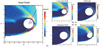 |
Fig. 2 Electromagnetic field components in the X − Z plane, where the panels represent the total field (a), convection field (b), Hall field (c), ambipolar field (d), and magnetic force field (e). The areas where the oxygen ion density is less than 0.001cm−3 have been blanked out. The field vectors are indicated by white arrows, and provide a clear visual depiction of the field dynamics across the plane. |
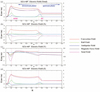 |
Fig. 3 Electromagnetic (EM) field and its components along the altitude at a zenith angle of 60° in the X − Z plane. Panels a–d display the magnitude of electric field, and the X, Y, and Z components of the electric field, respectively. The pink dashed lines mark the statistical positions of the MPB and BS. In the visualization, red represents the convection field, green denotes the Hall field, blue indicates the ambipolar field, black shows the magnetic force field, and pink illustrates the total field, including all components. |
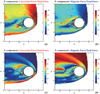 |
Fig. 4 Relative contributions of the EM field components in the X − Z plane. This figure quantifies the percentage of the convection electric field (panels a and c) and the magnetic force field (panels b and d) relative to the total field in the Z direction (panels a and b) and the X direction (panels c and d). The areas where the O+ ion density is below 0.001cm−3 have been blanked out. The black contour lines provide a visual representation of the field intensities across the plane. |
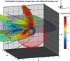 |
Fig. 5 Method for determining escape rates in the plume and the tail. The color plot represents common logarithms of radial escape fluxes of O+ ion. The solid black lines represent the MPB and BS (e.g., Vignes et al. 2000), while the black dotted line depicts a circle with radius of 6RM. The tailward escape is indicated by a red line and arrow, while the plume escape is denoted by a green line and arrow. |
3.2 Location and escape rate of the plume escape channel
To visualize O+ escape channels, Figure 5 represents the common logarithms of radial escape fluxes of O+ ion in the X − Z plane. It is clear that there are two escape channels highlighted by two strong flux regions. Figure 5 suggests that the O+ ion escape flux is relatively limited at low latitudes (0°–30°) within the northern hemisphere of the Martian meridian plane. In contrast, the escape flux intensifies at mid to high latitudes (30°–90°), which constitute the principal source region for the plume escape channel (e.g., Ma et al. 2023).
Rather than distinguishing between plume and tail region at locations close to Mars, it is better to perform calculations of the two escape rates at more distant locations. For this study, we evaluated and contrasted the rates of ion escape through the plume and tail region based on a sphere with a radius of 6RM, as shown in Figure 5, and illustrates the 3D diagram of calculating escape rates. The mesh represents the calculation region of escape rate. To distinguish between these regions, we used the intersection of the sphere with the MPB as the demarcation point, situated at Z = 6RM (e.g., Fang et al. 2008). Accordingly, we designated the plume region as the surface from Z = 3RM to 6RM (depicted as the green hemisphere) and the tail region as the surface from Z = −6RM to 3RM (depicted as the red hemisphere).
Using the demarcation point, the escape rates of O+ from plume and tail can be calculated to be approximately 4.33 × 10²³ s−1 and 1.74 × 1024 s−1, respectively. The corresponding total escape rate for O+ is therefore 2.18 × 1024 s−1. The plume escape is 24.83% of the tail escape and 19.89% of the total escape. The detailed calculations and comparative results are summarized in Table 1. Our simulated escape rates are consistent with Dong’s results from observations (e.g., Dong et al. 2015), and with the simulation results (e.g., Zhang et al. 2023).
A schematic plot of the plume escape, based on the conclusions of this paper, is presented in Figure 6, with the MPB and BS depicted by black lines. The various components of the EM field are represented by the colored arrows: green indicates the convection field, yellow represents the Hall field, blue signifies the ambipolar field, and the pink dashed line denotes the magnetic force field. The direction of the solar wind is marked by the red arrow. The color bar indicates common logarithms of radial escape fluxes of O+ ion.
Calculations and comparative results.
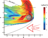 |
Fig. 6 Schematic diagram of the plume escape process. The colored arrows represent the components of electromagnetic field; green indicates the convection field, yellow represents the Hall field, blue signifies the ambipolar field, and the pink dashed line represents the magnetic force field. The direction of the solar wind is indicated by the red arrow, while the color bar represents the logarithmic scale of the O+ escape flux contour. |
4 Conclusions
In this study, we employed a three-dimensional multi-fluid MHD model to investigate the dynamic mechanism behind the ion plume escape process during the interaction between solar wind and Mars. The plume, which obtains energy from the electromagnetic field, primarily emerges outside the magnetic pileup boundary (MPB) in the +E hemisphere of the Mars-Sun-Electric field (MSE) coordinate system. According to the distribution characteristics of the field, we classified the plume structure into upstream and downstream plumes based on the bow shock (BS).
Our simulated study illustrates the plume with strong ion flux influenced by both the convection field and magnetic force field. In the dayside downstream plume, the convection field in the X direction accounts for 50% of the total field, with the magnetic force field contributing an equal percentage, but in the opposite vector direction. The Z component of the convection field dominates over 80%. The acceleration due to the convection field prevents pickup ions from precipitating back to Mars, creating a plume escape trajectory. In the upstream plume, the magnetic force field in the X direction causes ion deflection in the −X direction, resulting in the plume structure as detected by observation. The convection field in the Z direction further accelerates heavy ions, facilitating their escape from Mars. In addition, the Hall and ambipolar fields play crucial roles in the plume escape process, contributing approximately 20–30% of the total field near the MPB and BS. This study provides a more comprehensive and specific support for the variation of the plume influenced by alterations in the electric fields due to varying solar wind inputs.
We estimated the plume escape for O+ (4.33 × 10²³ s−1) to be 24.83% of the tail escape (1.74 × 1024 s−1) and 19.89% of the total escape (2.18 × 1024 s−1). The demarcation point distinguishing these channels is the intersection of the sphere (6RM) with the MPB, which is the innovative method we used. The comparison shows a good agreement between our approach and the previous results of simulation (e.g., Dong et al. 2015). It can also be seen that the plume channel located at mid to high latitudes in the +E hemisphere on the Martian dayside, which is consistent with statistical observations (e.g., Sakakura et al. 2022; Ma et al. 2023).
Acknowledgements
This work was supported by the National Natural Science Foundation of China under Grants 42241114, 42074214, and 12150008, the B-type Strategic Priority Program of the Chinese Academy of Sciences (Grant XDB41000000).
References
- Bougher, S. W., Engel, S., Roble, R. G., & Foster, B. 2000, JGRE, 105, 17669 [NASA ADS] [CrossRef] [Google Scholar]
- Dong, Y., Fang, X., Brain, D. A., et al. 2015, GeoRL, 42, 8942 [Google Scholar]
- Fang, X., Liemohn, M. W., Nagy, A. F., et al. 2008, JGRA, 113, A02210 [Google Scholar]
- Fang, X., Liemohn, M. W., Nagy, A. F., Luhmann, J. G., & Ma, Y. 2010, JGRA, 115, A04308 [Google Scholar]
- Fang, X., Ma, Y., Brain, D., Dong, Y., & Lillis, R. 2015, JGRA, 120, 10926 [Google Scholar]
- Gao, J. W., Rong, Z. J., Klinger, L., et al. 2021, E&SS, 8, e01860 [Google Scholar]
- Gunell, H., Maggiolo, R., Nilsson, H., et al. 2018, A&A, 614, L3 [NASA ADS] [CrossRef] [EDP Sciences] [Google Scholar]
- Hinton, P. C., Brain, D. A., Schnepf, N. R., Jarvinen, R., & Ramstad, R. 2024, MNRAS, 533, 3999 [Google Scholar]
- Jarvinen, R., Brain, D. A., & Luhmann, J. G. 2016, P&SS, 127, 1 [Google Scholar]
- Jarvinen, R., Brain, D. A., Modolo, R., Fedorov, A., & Holmstrom, M. 2018, JGRA, 123, 1678 [Google Scholar]
- Johnson, B. C. 2018, Mars’ Energetic Plume Ion Escape Channel, University of Michigan [Google Scholar]
- Li, Y., Lu, H., Cao, J., et al. 2021, ApJ, 921, 139 [NASA ADS] [CrossRef] [Google Scholar]
- Li, S., Lu, H., Cao, J., et al. 2022, ApJ, 941, 198 [NASA ADS] [CrossRef] [Google Scholar]
- Li, S.-b., Lu, H.-y., Cao, J.-b., et al. 2023, AdSpR, 72, 3212 [Google Scholar]
- Liu, D., Rong, Z. J., Gao, J. W., et al. 2021, ApJ, 911, 113 [NASA ADS] [CrossRef] [Google Scholar]
- Ma, X., Tian, A., Guo, R., et al. 2023, Icarus, 406, 540 [Google Scholar]
- Ma, Y. J., Nagy, A. F., Sokolov, I. V., & Hansen, K. C. 2004, JGRA, 109, A07211 [NASA ADS] [Google Scholar]
- Ma, Y. J., Dong, C. F., Toth, G., et al. 2019, JGRA, 124, 9040 [Google Scholar]
- Najib, D., Nagy, A. F., Toth, G., & Ma, Y. 2011, JGRA, 116, A05204 [NASA ADS] [CrossRef] [Google Scholar]
- Orosei, R., Lauro, S. E., Pettinelli, E., et al. 2018, Science, 361, 490 [Google Scholar]
- Sakakura, K., Seki, K., Sakai, S., et al. 2022, JGRA, 127, e2021JA029750 [Google Scholar]
- Song, Y., Lu, H., Cao, J., et al. 2023, JGRA, 128, e2022JA031083 [NASA ADS] [Google Scholar]
- Vignes, D., Mazelle, C., Rme, H., et al. 2000, GeoRL, 27, 49 [Google Scholar]
- Xu, S., Mitchell, D. L., Ma, Y., et al. 2021, JGRA, 126, e29764 [Google Scholar]
- Zhang, Q., Holmstrom, M., Wang, X.-d., Nilsson, H., & Barabash, S. 2023, JGRA, 128, e2023JA031828 [NASA ADS] [Google Scholar]
All Tables
All Figures
|
Fig. 1 Density and velocity of O+ ions in the X − Z Plane. The color plot represents ion density; the areas where the oxygen ion density is less than 0.001cm−3 have been blanked out. The white lines represent the magnetic pileup boundary (MPB, internally) and the bow shock (BS, externally) according to the empirical model by Vignes et al. (2000). The arrows depict the velocity vectors of O+ ions. |
| In the text | |
|
Fig. 2 Electromagnetic field components in the X − Z plane, where the panels represent the total field (a), convection field (b), Hall field (c), ambipolar field (d), and magnetic force field (e). The areas where the oxygen ion density is less than 0.001cm−3 have been blanked out. The field vectors are indicated by white arrows, and provide a clear visual depiction of the field dynamics across the plane. |
| In the text | |
|
Fig. 3 Electromagnetic (EM) field and its components along the altitude at a zenith angle of 60° in the X − Z plane. Panels a–d display the magnitude of electric field, and the X, Y, and Z components of the electric field, respectively. The pink dashed lines mark the statistical positions of the MPB and BS. In the visualization, red represents the convection field, green denotes the Hall field, blue indicates the ambipolar field, black shows the magnetic force field, and pink illustrates the total field, including all components. |
| In the text | |
|
Fig. 4 Relative contributions of the EM field components in the X − Z plane. This figure quantifies the percentage of the convection electric field (panels a and c) and the magnetic force field (panels b and d) relative to the total field in the Z direction (panels a and b) and the X direction (panels c and d). The areas where the O+ ion density is below 0.001cm−3 have been blanked out. The black contour lines provide a visual representation of the field intensities across the plane. |
| In the text | |
|
Fig. 5 Method for determining escape rates in the plume and the tail. The color plot represents common logarithms of radial escape fluxes of O+ ion. The solid black lines represent the MPB and BS (e.g., Vignes et al. 2000), while the black dotted line depicts a circle with radius of 6RM. The tailward escape is indicated by a red line and arrow, while the plume escape is denoted by a green line and arrow. |
| In the text | |
|
Fig. 6 Schematic diagram of the plume escape process. The colored arrows represent the components of electromagnetic field; green indicates the convection field, yellow represents the Hall field, blue signifies the ambipolar field, and the pink dashed line represents the magnetic force field. The direction of the solar wind is indicated by the red arrow, while the color bar represents the logarithmic scale of the O+ escape flux contour. |
| In the text | |
Current usage metrics show cumulative count of Article Views (full-text article views including HTML views, PDF and ePub downloads, according to the available data) and Abstracts Views on Vision4Press platform.
Data correspond to usage on the plateform after 2015. The current usage metrics is available 48-96 hours after online publication and is updated daily on week days.
Initial download of the metrics may take a while.