| Issue |
A&A
Volume 698, June 2025
|
|
|---|---|---|
| Article Number | A187 | |
| Number of page(s) | 10 | |
| Section | Planets, planetary systems, and small bodies | |
| DOI | https://doi.org/10.1051/0004-6361/202554525 | |
| Published online | 13 June 2025 | |
The influence of external solar-wind drivers on the physical characteristics of the Martian bow shock
1
School of Space and Earth Sciences, Beihang University,
Beijing,
China
2
Key Laboratory of Space Environment Monitoring and Information Processing, Ministry of Industry and Information Technology,
Beijing,
China
3
Institut de Recherche en Astrophysique et Planétologie (IRAP), CNRS, Université de Toulouse, CNES,
Toulouse,
France
4
Planetary Environmental and Astrobiological Research Laboratory (PEARL), School of Atmospheric Sciences, Sun Yat-sen University, Zhuhai,
Guangdong,
China
5
Chinese Academy of Sciences Center for Excellence in Comparative Planetology, Hefei,
Anhui,
China
6
Institute of Geology and Geophysics, Chinese Academy of Sciences,
Beijing,
China
★ Corresponding author: This email address is being protected from spambots. You need JavaScript enabled to view it.
Received:
14
March
2025
Accepted:
5
May
2025
Abstract
The Martian bow shock represents the main interface between the upstream interplanetary space and the downstream planetary obstacle, where the solar-wind plasma and the frozen-in interplanetary magnetic field (IMF) begin to be perturbed. However, the physical characteristics of the Martian bow shock layer and the influence of the external solar wind drivers on them remain unclear. By employing a three-dimensional Hall magneto-hydrodynamic (MHD) model, this study aims to reveal the physical characteristics of the Martian bow-shock layer extracted from the maximum radially inward gradient of the solar-wind velocity (VS W), including the magnetic field, current density, electric fields, and the energy transfer between the fields and solar wind protons, as well as the influence of the VS W and the IMF on these features. Simulation results indicate that the IMF has initiated the processes of piling-up, draping, bending, and slipping at the Martian bow shock, inducing an associate current to flow from the +ZMS E pole to the −ZMS E pole along the bow-shock layer, with the strongest being located at the subsolar position. Furthermore, the total electric field at the Martian bow shock is constituted by the motional electric field (EM) with the +ZMS E direction around the ±ZMS E flanks and the outward ambipolar (EA) and Hall (EH) electric fields around the lower solar zenith angles; through these, the solar wind transfers its kinetic energy to the electromagnetic fields. A higher VS W gives rise to an enhanced magnetic field, current density, and electric fields at the Martian bow shock, thereby leading to an increase in the corresponding energy-transfer rates. A greater magnitude of the IMF cross-flow component tends to result in an intensified magnetic field, current densities, EM, and EH; while it causes a decreased EA and associated energy-transfer rate at the bow shock layer. If the Parker spiral angle of the IMF is not restricted to 90°, a portion of the quasi-parallel bow-shock layer will be formed, within which the magnitudes of the magnetic field, current density, EH, and the corresponding energy-transfer rate through EH are all lower than those of the quasi-perpendicular bow-shock layer. The results of this study provide valuable insights into the physical properties at the bow-shock layer that emerge during the Mars-solar-wind interactions.
Key words: magnetohydrodynamics (MHD) / methods: numerical / planets and satellites: terrestrial planets
© The Authors 2025
 Open Access article, published by EDP Sciences, under the terms of the Creative Commons Attribution License (https://creativecommons.org/licenses/by/4.0), which permits unrestricted use, distribution, and reproduction in any medium, provided the original work is properly cited.
This article is published in open access under the Subscribe to Open model. This email address is being protected from spambots. You need JavaScript enabled to view it. to support open access publication.
1 Introduction
The solar wind, which is composed of the solar coronal plasma, is a supersonic stream of flow that pervades the entire Solar System. Upon colliding with the planetary obstacle, the solar wind is decelerated and deflected to form a comet-like cavity, which is isolated from interplanetary space by the bow shock. Therefore, planetary bow shocks indicate the area where the interplanetary solar wind flow begins to be disturbed due to the existence of a downstream planetary obstacle, such as its magnetosphere or atmosphere. The exploration of planetary bow shocks provides significant insights not only into the effect of the collisionless shocks, but also into the nature of the planetary obstacles.
The interaction between the solar wind and Mars presents a unique pattern in our Solar System, as the Martian ionosphere and induced magnetosphere constitute the main obstacle to the solar wind. This is because Mars lacks a global intrinsic dynamo magnetic field but has remnant crustal fields mainly located in its southern hemisphere (Acuna et al. 1999). Additionally, its comparatively small size and greater heliocentric distance and lower mass and gravity exert substantial implications on the shock characteristics (Mazelle et al. 2004).
As the outermost boundary of the Martian space environment, the Martian bow shock was first reported by the Mariner 4 flyby (Smith et al. 1965) and Mars 2, 3, and 5 orbiters (Russell 1977, 1978a,b). Subsequently, based on the abundant magnetic field and plasma data provided by Phobos-2, the existence of the Martian bow shock was affirmed, and the associated shape was revealed through statistical data fit by the conic section function (Riedler et al. 1989; Trotignon et al. 1991a,b, 1993). However, the bow-shock crossings of Phobos-2 are mainly concentrated on the far magnetotail, which is greater than 10 RM. It was not until the Mars Global Surveyor (MGS) that sufficient dayside crossings of the Martian bow shock were performed, thereby confirming that the average subsolar and terminator distances of the bow shock are approximately 1.58 RM and 2.6 RM (Vignes et al. 2000; Trotignon et al. 2006; Edberg et al. 2008). With an increasing availability of more precise observation data from the Mars Express (MEX, Dubinin et al. 2006; Edberg et al. 2009; Hall et al. 2016) and the Mars Atmosphere and Volatile EvolutioN (MAVEN, Jakosky et al. 2015; Connerney et al. 2015), global parametric Martian bow-shock models employing a generalized conic section function were developed to investigate the shape and location of the shock in correspondence with the variations of the upstream and downstream conditions (Ramstad et al. 2017; Gruesbeck et al. 2018; Wang et al. 2020). However, these models are more focused on the locations of the Martian bow shock rather than the physical features on the shock surface, which play a crucial role in the Mars-solar-wind interaction.
The Martian bow shock exhibits distinct physical characteristics during the Mars-solar-wind interaction, including solar-wind velocity (VS W), magnetic field, current density, electric field, and associated energy transfer. As the supersonic solar wind encounters the Martian obstacle, it decelerates, deflects, and compresses, resulting in the piling-up and wrapping of the frozen-in interplanetary magnetic field (IMF) at the bow shock. This enhancement and bending of the IMF tend to induce a current layer, mainly in the direction opposite to the solar-wind motional electric field. Furthermore, electric fields emerge as a consequence of charge separation between ions and electrons at the bow shock, through which the plasma kinetic energy is transferred to the thermal and electromagnetic-field energy, signifying that the Martian bow shock functions as the most powerful dynamo region for energy input (Ramstad et al. 2020; Wang et al. 2023, 2024).
Upstream solar-wind conditions not only influence the location and shape of the Martian bow shock, they also have an impact on its physical characteristics. The dynamic pressure of the solar wind is one of the dominant factors influencing the configuration of the Martian bow shock. High solar-wind dynamic pressure is capable of compressing the Martian bow shock to a lower altitude, resulting in the average position of the bow shock moving toward the planet and a reduction in the flaring angle of the bow shock (Hall et al. 2016; Halekas et al. 2017; Gruesbeck et al. 2018; Wang et al. 2020). However, the subsolar stand-off distance and the flaring angle of the Martian bow shock tend to increase in accordance with the strength of the cross-flow component of the IMF (Sui et al. 2023; Wang et al. 2020). In addition, the direction of the IMF (cone angle and clock angle) can give rise to asymmetry on the bow-shock surface; that is, the bow shock on the quasi-parallel side is nearer to Mars than that on the quasi-perpendicular side (Yuan et al. 2024; Garnier et al. 2022a; Zhang et al. 1991). Unfortunately, the physical characteristics of the bow-shock layer have barely been presented by these parametric Martian bow-shock models, let alone the impact of the external solar-wind drivers on these characteristics. Recent simulations have revealed that the magnitudes of corresponding electromagnetic forces at the Martian bow shock increase simultaneously to balance the enhanced solar-wind dynamic pressure, driving the location of the bow shock toward Mars (Song et al. 2023a). However, the simulation results displayed limited physical characteristics at the bow shock, mainly due to presenting the boundary in two-dimensional planes, despite the employment of a three-dimensional simulation.
Therefore, in this study, the Martian bow-shock layer is extracted from the three-dimensional multi-fluid Hall-MHD simulation domain to reveal its comprehensive characteristics, including magnetic field, current density, electric fields, and energy transfer at the boundary layer, as well as the impact of the VS W and IMF on these characteristics. The subsequent sections of this paper are structured as follows: Section 2 provides a description of the multi-fluid Hall-MHD model, Section 3 shows the simulation results, and Section 4 summarizes our study.
2 Model description
With the extensive application and development of computational hydrodynamics, this method is also being increasingly utilized in space science. However, in the Universe, the fluids are magnetized and thus subject to interaction with the electromagnetic environment of the surrounding space. Accordingly, to capture the fluid dynamics of each ion species (![Mathematical equation: $\[\mathrm{H}^{+}, \mathrm{O}_{2}^{+}, \mathrm{O}^{+}, \mathrm{CO}_{2}^{+}\]$](/articles/aa/full_html/2025/06/aa54525-25/aa54525-25-eq1.png) ), the multi-fluid Hall-MHD model, which regards each ion species as a separate fluid coupled to the magnetic-induction equation including the Hall term, has been developed and proven to be a computationally efficient and reliable method for modeling the Mars-solar-wind interactions (Li et al. 2020, 2022a,b, 2024b, 2025; Song et al. 2023a,b, 2025; Najib et al. 2011; Dong et al. 2014, 2015; Ma et al. 2019).
), the multi-fluid Hall-MHD model, which regards each ion species as a separate fluid coupled to the magnetic-induction equation including the Hall term, has been developed and proven to be a computationally efficient and reliable method for modeling the Mars-solar-wind interactions (Li et al. 2020, 2022a,b, 2024b, 2025; Song et al. 2023a,b, 2025; Najib et al. 2011; Dong et al. 2014, 2015; Ma et al. 2019).
During the process of performing the multi-fluid Hall-MHD model for simulating the interaction between the solar-wind and Martian atmospheres, by setting appropriate solar-wind conditions, the self-consistent generation of four ion species (![Mathematical equation: $\[\mathrm{H}^{+}, \mathrm{O}_{2}^{+}, \mathrm{O}^{+}, \mathrm{CO}_{2}^{+}\]$](/articles/aa/full_html/2025/06/aa54525-25/aa54525-25-eq2.png) ) can be achieved by integrating an atmospheric profile (H, O, CO2) (Bougher et al. 2001) and taking into account the solar extreme-ultraviolet flux (Huestis 2001), as well as considering the physical collisions and chemical reactions among them (Schunk & Nagy 2009). Subsequently, the characteristics of individual ion species within the Martian space environment can be precisely captured by solving a series of gas-dynamic Euler equations related to their mass, momentum, and energy under the second-order entropy-conditioned scheme (Dong et al. 2002). Additionally, the temporal evolution of the Martian electromagnetic environments is derived by solving the magnetic-induction equation computed using a second-order MacCormack scheme (MacCormack 2003). Previous simulation-observation comparisons carried out by Song et al. (2023b) confirmed that the ionospheric ion densities and dynamics depicted by the Hall-MHD model reproduce the characteristics of the Martian ionosphere precisely. Furthermore, when taking the MAVEN measurements of the solar wind as the initial input and inter-polating the quasi-steady simulation results onto the orbit of the MAVEN satellite, the direct comparison between the simulation results and observational data demonstrated relatively good consistencies, thereby validating the multi-fluid Hall-MHD model (see the appendix in Li et al. 2023). The equations governing the multi-fluid Hall-MHD model can be expressed as follows:
) can be achieved by integrating an atmospheric profile (H, O, CO2) (Bougher et al. 2001) and taking into account the solar extreme-ultraviolet flux (Huestis 2001), as well as considering the physical collisions and chemical reactions among them (Schunk & Nagy 2009). Subsequently, the characteristics of individual ion species within the Martian space environment can be precisely captured by solving a series of gas-dynamic Euler equations related to their mass, momentum, and energy under the second-order entropy-conditioned scheme (Dong et al. 2002). Additionally, the temporal evolution of the Martian electromagnetic environments is derived by solving the magnetic-induction equation computed using a second-order MacCormack scheme (MacCormack 2003). Previous simulation-observation comparisons carried out by Song et al. (2023b) confirmed that the ionospheric ion densities and dynamics depicted by the Hall-MHD model reproduce the characteristics of the Martian ionosphere precisely. Furthermore, when taking the MAVEN measurements of the solar wind as the initial input and inter-polating the quasi-steady simulation results onto the orbit of the MAVEN satellite, the direct comparison between the simulation results and observational data demonstrated relatively good consistencies, thereby validating the multi-fluid Hall-MHD model (see the appendix in Li et al. 2023). The equations governing the multi-fluid Hall-MHD model can be expressed as follows:
![Mathematical equation: $\[\frac{\partial \rho_s}{\partial t}+\nabla \bullet\left(\rho_s \boldsymbol{u}_s\right)=\frac{\delta \rho_s}{\delta t},\]$](/articles/aa/full_html/2025/06/aa54525-25/aa54525-25-eq3.png) (1)
(1)
![Mathematical equation: $\[\begin{aligned}& \frac{\partial\left(\rho_s ~\boldsymbol{u}_s\right)}{\partial t}+\nabla \bullet\left(\rho_s ~\boldsymbol{u}_s ~\boldsymbol{u}_s+\boldsymbol{I} p_s\right) \\& =n_s ~q_s\left(\boldsymbol{u}_s-\boldsymbol{u}_{+}\right) \times \boldsymbol{B}+\frac{n_s ~q_s}{n_e ~e}\left(\boldsymbol{J} \times \boldsymbol{B}-\nabla p_e\right)+\frac{\delta M_s}{\delta t},\end{aligned}\]$](/articles/aa/full_html/2025/06/aa54525-25/aa54525-25-eq4.png) (2)
(2)
![Mathematical equation: $\[\begin{aligned}& \frac{\partial e_s}{\partial t}+\nabla \bullet\left[\left(e_s+p_s\right) \boldsymbol{u}_s\right] \\& =\boldsymbol{u}_s \bullet\left[n_s ~q_s\left(\boldsymbol{u}_s-\boldsymbol{u}_{+}\right) \times \boldsymbol{B}+\frac{n_s ~q_s}{n_e ~e}\left(\boldsymbol{J} \times \boldsymbol{B}-\nabla p_e\right)\right]+\frac{\delta E_s}{\delta t},\end{aligned}\]$](/articles/aa/full_html/2025/06/aa54525-25/aa54525-25-eq5.png) (3)
(3)
![Mathematical equation: $\[\frac{\partial \boldsymbol{B}}{\partial t}-\nabla \times\left(\boldsymbol{u}_{+} \times \boldsymbol{B}-\frac{\boldsymbol{J} \times \boldsymbol{B}}{e n_e}+\frac{\nabla p_e}{e n_e}\right)=0,\]$](/articles/aa/full_html/2025/06/aa54525-25/aa54525-25-eq6.png) (4)
(4)
where Eqs. (1)–(3) represent the conservative Euler equations and Eq. (4) stands for the magnetic-induction equation. Here, ρs, us, ps, ns, and qs are the individual mass density, velocity, pressure, number density, and charge of the species s, respectively. I is the identity matrix, ![Mathematical equation: $\[e_{s}=\frac{1}{2} \rho_{s} \boldsymbol{u}_{s}^{2}+\frac{p_{s}}{\gamma-1}\]$](/articles/aa/full_html/2025/06/aa54525-25/aa54525-25-eq7.png) , and γ is the polytropic index chosen to be 5/3. pe = ∑i=ions pi and ne = ∑i=ions ni are the pressure and number density of electrons. u+ is the charge-averaged ion velocity:
, and γ is the polytropic index chosen to be 5/3. pe = ∑i=ions pi and ne = ∑i=ions ni are the pressure and number density of electrons. u+ is the charge-averaged ion velocity: ![Mathematical equation: $\[\frac{1}{e n_{e}} \sum_{s} n_{s} q_{s} \boldsymbol{u}_{s}\]$](/articles/aa/full_html/2025/06/aa54525-25/aa54525-25-eq8.png) . The electric current density can be obtained from
. The electric current density can be obtained from ![Mathematical equation: $\[\boldsymbol{J}=\frac{1}{\mu_{0}} \nabla \times \boldsymbol{B}\]$](/articles/aa/full_html/2025/06/aa54525-25/aa54525-25-eq9.png) . Moreover, as demonstrated in Eqs. (1)–(4), the total electric field (ET) is composed of the motional electric field (EM = −u+ × B), the Hall electric field
. Moreover, as demonstrated in Eqs. (1)–(4), the total electric field (ET) is composed of the motional electric field (EM = −u+ × B), the Hall electric field ![Mathematical equation: $\[\left(\boldsymbol{E}_{H}=\frac{\boldsymbol{J} \times \boldsymbol{B}}{e n_{e}}\right)\]$](/articles/aa/full_html/2025/06/aa54525-25/aa54525-25-eq10.png) , and the ambipolar electric field
, and the ambipolar electric field ![Mathematical equation: $\[\left(\boldsymbol{E}_{A}=-\frac{\nabla p_{e}}{e n_{e}}\right)\]$](/articles/aa/full_html/2025/06/aa54525-25/aa54525-25-eq11.png) . The source terms
. The source terms ![Mathematical equation: $\[\frac{\delta \rho_{s}}{\delta t}, \frac{\delta M_{s}}{\delta t}\]$](/articles/aa/full_html/2025/06/aa54525-25/aa54525-25-eq12.png) , and
, and ![Mathematical equation: $\[\frac{\delta E_{s}}{\delta t}\]$](/articles/aa/full_html/2025/06/aa54525-25/aa54525-25-eq13.png) on the rightmost side of Eqs. (1)–(3) represent the variations in mass, momentum, and energy of the ion species that arise from physical collisions and chemical reactions among all species (Schunk & Nagy 2009; Najib et al. 2011; Li et al. 2020).
on the rightmost side of Eqs. (1)–(3) represent the variations in mass, momentum, and energy of the ion species that arise from physical collisions and chemical reactions among all species (Schunk & Nagy 2009; Najib et al. 2011; Li et al. 2020).
A spherical simulation grid composed of 960 000 cells within the Mars-centered Solar Orbital (MSO) coordinate frame was employed in our simulation, where the X-axis (−24 RM ≤ X ≤ 8 RM, RM ≈ 3396 km is the radius of Mars) points from Mars toward the Sun, with the Z-axis (−16 RM ≤ Z ≤ 16 RM) being perpendicular to the X-axis and positively oriented toward the north celestial pole. The Y-axis (−16 RM ≤ Y ≤ 16 RM) completes the right-hand coordinate system. Since the general curvilinear coordinate system was adopted and transformed from the physical MSO coordinate system, high resolution for the region with intense variations of physical parameters can be achieved by refining the physical grid. The inner boundary, which is 100 km above the Martian surface, has a minimum grid size of 10 km. At this boundary, it is assumed that the ion velocities are zero and the densities are at photochemical equilibrium values; meanwhile, the density of H+ is regarded as 0.3 times that of the densities of solar-wind protons (Dong et al. 2014, 2015). The subsolar location corresponds to the 180° W at the equator.
To explore the influence of the VS W and IMF on the physical properties of the Martian bow shock, we conducted four simulation cases under diverse VS W and IMF with a solar-wind density of 4 cm−3 and a proton temperature of 3.5 × 10⁵ K. The specific parameters of each case are presented in Table 1. Simulation Case 1 was devised to reveal the physical characteristics at the Martian bow shock under normal solar wind conditions. For Cases 2 and 3, the magnitudes of the VS W and IMF cross-flow component (By) were separately augmented by a factor of two, thereby exploring the individual impacts of their intensities on the physical properties of the bow-shock layer. Additionally, in simulation Case 4, an IMF Parker spiral angle of 56° was adopted to investigate the influence of the IMF direction. The magnetosonic Mach number (MM S) in Case 2 doubled to 14, whereas in Case 3 it decreased to 5.5, as compared with Case 1. Hence, Case 2 also represents a high MM S circumstance arising from a high magnitude of VS W, while Case 3 also represents a low MM S situation due to high IMF strength. These upstream solar-wind conditions listed in Table 1 indicate that the directions of VS W and EM in all simulation cases are aligned along the X-axis and Z-axis under the MSO coordinates. Consequently, the Mars Solar Electric (MSE) coordinates are identical to the MSO in these simulations, where ZMS E is parallel to the EM, XMS E points from Mars toward the Sun, and YMS E completes the right-handed coordinate system. Our simulation results are presented in the MSE coordinate to obtain more generalized conclusions related to the EM and to facilitate comparisons with the previous statistical observations. It should be noted that the simulations were carried out without taking the Martian crustal fields into account, with the specific aim of revealing the induced physical characteristics at the bow shock layer and exploring the impact of the external solar-wind drivers on these properties.
Settings of upstream solar-wind velocity (VS W) and interplanetary magnetic field (IMF) as well as corresponding magnetosonic Mach number (MM S) in the simulation cases.
3 Simulation results
3.1 Physical characteristics at the Martian bow shock
Firstly, we explored the physical properties of the Martian bow shock under normal solar-wind conditions (Case 1). In order to reveal the physical characteristics at the Martian bow shock, the extraction of the bow-shock layer from the numerical simulation domain is required. Based on Rankine-–Hugoniot relations, Fang et al. (2015) proposed an automatic algorithm to identify the three-dimensional locations of the dayside bow shock by utilizing the peaks of the plasma speed gradient along the radial direction. In this study, we employed this criterion to extract the locations of the dayside bow-shock layer, where the radially inward gradient of the solar-wind velocity is maximized.
Figure 1a presents the distribution of the VS W in the XY plane, along with its vectors. It is obvious that when supersonic solar wind plasma encounters the Martian obstacle, it tends to be decelerated and deflected, forming a bow shock in front of the planet accompanied by two symmetrical magnetotail lobes. The radial gradient of the VS W in the XY plane is depicted in Fig. 1b, overlapping with the average locations of the bow shock (white dashed line) as adopted from Vignes et al. (2000). It can be observed that the locations where the radial gradient of VS W is at its maximum essentially coincides with the statistical average positions of the Martian bow shock. Furthermore, the distributions of the VS W and the corresponding radial gradient in the XZ plane are demonstrated in Figs. 1c and 1d, respectively, which exhibit similar characteristics to Figs. 1a and 1b; however, the solar wind plasma tends to shift toward the −ZMS E magnetotail due to the magnetic forces arising from the bending of the IMF over the polar region (Chai et al. 2019; Dubinin et al. 2019; Li et al. 2024a). To identify the locations of the dayside Martian bow shock (X > 0), the maximum values of the radially inward gradient of the VS W are extracted from the simulation results of Case 1, as depicted in Fig. 1e, where the VS W is mapped in conjunction with its vectors. It is obvious that the solar-wind flow is deflected in all directions, with the minimum velocity occurring in the vicinity of the subsolar position, reproducing the phenomenon where the solar-wind plasma decelerates and deflects at the Martian-bow-shock layer. To display the comprehensive features of the dayside Martian-bow-shock layer, it is preferable to view it from the Sun; this is presented in Fig. 1f, which shows the XMS E positions of the bow shock along with three corresponding contour lines. It can be observed from Fig. 1f that the bow shock exhibits ±YMS E symmetrical distribution under the upstream solar-wind conditions of simulation Case 1. However, an asymmetrical distribution exists around the ±ZMS E terminator flanks primarily due to the failure of the radial gradient criterion at these positions (Fang et al. 2015); yet, this does not impede the investigation of the physical characteristics on the dayside Martian bow shock.
To investigate the distribution of the IMF at the Martian-bow-shock layer, Fig. 2a1 depicts the color-coded bow shock based on the magnetic-field strength and overlapped with its vectors. Besides this, the distributions of its components Bx, By, and Bz at the boundary layer are, respectively, provided in Figs. 2a2–2a4. It is evident from Figs. 2a1–a4 that the magnetic fields at the Martian bow shock are mainly composed of the IMF By component with a magnitude of approximately 8 nT, which is nearly three times that of the upstream IMF. This enhancement of the magnetic field indicates that the IMF has begun to pile up at the bow-shock layer as the solar-wind flow slows down. Meanwhile, the −YMS E (+YMS E) bow-shock layer features +Bx (−Bx) as depicted in Fig. 2a2, suggesting that the magnetic fields undergo draping and bending as the solar-wind flow deflects. Another characteristic of the IMF topology can be mirrored by the Bz component as shown in Fig. 2a4, which exhibits a symmetrical quadrupole pattern (Bz · YMS E · ZMS E < 0), indicating that IMFs tend to symmetrically slip at the bow-shock layer over its ±ZMS E poles. Therefore, the magnetic fields frozen in the solar-wind flow at the Martian bow-shock layer display complex behaviors, such as piling up, draping, bending, and slipping.
According to ![Mathematical equation: $\[\boldsymbol{J}=\frac{1}{\mu_{0}} \nabla \times \boldsymbol{B}\]$](/articles/aa/full_html/2025/06/aa54525-25/aa54525-25-eq14.png) , the current density is correlated with the magnetic fields. Consequently, the intricate behaviors of the IMFs within the Martian-bow-shock layer are capable of inducing a current layer, as depicted in Figs. 2b1–b4, where the distributions of the total and the corresponding three components of the current density at the bow-shock layer are presented along with its vectors. It is obvious that the current density is predominantly in the −ZMS E direction, flowing from the +ZMS E pole to the −ZMS E pole along the bow-shock layer, with the maximum magnitude of approximately 40 nA/m2 around the subsolar area. However, the maximum value of the current density is up to twice as strong as the statistical value reported by Ramstad et al. (2020). This discrepancy is anticipated as the statistical study averaging over 9000 orbits fails to resolve the bow-shock structure smaller than 0.2 RM, whereas this study reveals the bow-shock current layer at the ion scale. A similar noticeable difference also exists in the investigation of the current layer within the Martian magnetic pile up boundary (Boscoboinik et al. 2023), which highlights that the study of the Martian current system should be at ion scales.
, the current density is correlated with the magnetic fields. Consequently, the intricate behaviors of the IMFs within the Martian-bow-shock layer are capable of inducing a current layer, as depicted in Figs. 2b1–b4, where the distributions of the total and the corresponding three components of the current density at the bow-shock layer are presented along with its vectors. It is obvious that the current density is predominantly in the −ZMS E direction, flowing from the +ZMS E pole to the −ZMS E pole along the bow-shock layer, with the maximum magnitude of approximately 40 nA/m2 around the subsolar area. However, the maximum value of the current density is up to twice as strong as the statistical value reported by Ramstad et al. (2020). This discrepancy is anticipated as the statistical study averaging over 9000 orbits fails to resolve the bow-shock structure smaller than 0.2 RM, whereas this study reveals the bow-shock current layer at the ion scale. A similar noticeable difference also exists in the investigation of the current layer within the Martian magnetic pile up boundary (Boscoboinik et al. 2023), which highlights that the study of the Martian current system should be at ion scales.
The electric fields at the Martian bow shock exert the direct force that decelerates the solar-wind protons, through which the kinetic energy of the solar wind is transferred to the electromagnetic fields. The distributions of the total electric field (ET), which is composed of the motional (EM), Hall (EH), and ambipolar (EA) electric fields, along with the associated energy-transfer rates between the solar wind protons, are demonstrated in Fig. 3. It is evident that the directions of the EM predominantly point toward the +ZMS E, resulting in the concentration of the EM on the ±ZMS E flanks with a magnitude of approximately 2.5 V /km. The symmetrical draping and slipping patterns of the IMF at the Martian bow shock give rise to the symmetrical distribution of the outward EH, with the maximum magnitude of 0.2 V /km around the subsolar region, and it gradually decays as the solar zenith angle (SZA) increases. Furthermore, EA exhibits similar distribution characteristics to EH, but possesses a significantly stronger magnitude of 2.5 V /km at the subsolar position, which is consistent with results of previous studies (Xu et al. 2021; Wang et al. 2023). Accordingly, the electric field at the Martian bow shock is attributed to the EM pointing toward the +ZMS E around ±ZMS E flanks, accompanied by outward EA and EH around the lower SZA area.
The spatial distributions of the solar-wind proton energy-transfer rates can reveal the details of the energy transfer between the fields and the solar-wind plasmas at the Martian bow shock, as shown in the right column of Fig. 3. The significant negative-energy-transfer rate between the total electric-field and solar-wind protons (ET · JH+ < 0), as depicted in Fig. 3b1, implies that the Martian bow shock acts as a substantial dynamo, through which the kinetic energy of the solar wind is efficiently converted into electromagnetic energy. This is in accordance with the previous hybrid simulation results, which indicated that the bow shock is the most powerful dynamo of energy input, where the plasma energy of the solar wind is transferred to the electromagnetic field at a rate of about −1 × 10⁻¹⁰ ~ −10 × 10−10 W / m3. However, they only revealed the energy transfer between the total electric field and various ion species, but there exist discrepancies in the energy-transfer patterns between different electric-field terms and various ion species (Li et al. 2024b, 2025). From the energy transfer between the EM and the solar wind (Fig. 3b2), it can be deduced that the solar wind predominantly transfers its energy to the EM around the +ZMS E pole, at rates of approximately −0.15 × 10⁻¹⁰ W / m3, which is extremely low in comparison with the total energy-transfer rates. However, the transfer of the kinetic energy of the solar wind to the EA and EH mainly occurs around the subsolar region, with maximum rates of −10 × 10−10 W / m3 and −1 × 10⁻¹⁰ W / m3, respectively, and gradually decays as the SZA increases. In conclusion, it can be inferred that the kinetic energy of the solar wind plasma is transferred to the electromagnetic field at the Martian bow shock, with the vast majority being converted into EA and a small proportion into EH around the lower SZAs. An extremely small proportion are converted into EM around the +ZMS E pole.
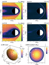 |
Fig. 1 Distribution of solar-wind velocity in (a) XY and (c) XZ planes for Case 1, overlapping with its vectors. The distribution of the radial gradient of the solar-wind velocity in the (b) XY and (d) XZ planes for Case 1 is shown overlapping with dashed average bow-shock locations (Vignes et al. 2000). (e) Martian-bow-shock layer colored based on the magnitude of the solar-wind velocity and overlapping with its vectors for Case 1. (f) Locations of XMS E at Martian-bow-shock layer for Case 1 along with three corresponding contoured solid lines, as viewed from the Sun. |
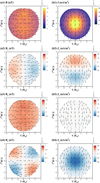 |
Fig. 2 Distribution of (a1) total magnetic-field magnitude and (a2, a3, a4) its components (Bx, By, Bz) at the Martian bow-shock layer for Case 1, overlapping with magnetic-field vectors. The distribution of (b1) total current density magnitude and (b2, b3, b4) its components (Jx, Jy, Jz) at the bow-shock layer for Case 1, overlapping with current vectors. |
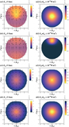 |
Fig. 3 Distribution of (a1) total electric-field overlapping with its uniform vectors and (a2) its energy-transfer rate between solar-wind protons at the Martian bow shock for Case 1. The distributions of (b1–b2) motional, (c1–c2) Hall, and (d1–d2) ambipolar electric fields at the bow-shock layer for Case 1, along with the associated energy transfer rates, are presented in a format consistent with that used for the a1–a2 total electric-field. |
3.2 The influence of the magnitude of VSW
When the upstream VS W doubles, the shape of the Martian bow shock is significantly compressed as a result of the higher MM S, as inferred from the gradient of the VS W depicted in Figs. 4a, b. More specifically, the subsolar position of the bow shock decreases to 1.48 RM, in contrast to the corresponding 1.58 RM in Case 1; and the terminator position compresses to 2.4 RM, as compared to the corresponding 2.7 RM in Case 1, which are consistent with the previous conclusions drawn from the parametric bow-shock model (Wang et al. 2020; Garnier et al. 2022a). To extract the Martian-bow-shock layer from the simulation results of Case 2, we still adopted the criterion of the maximum value of the radially inward gradient of VS W to determine the location of the bow shock. Figure 4c presents the bow-shock layer derived from simulation Case 2, which is colored according to the magnitude of VS W and overlaps its vectors. It is manifest that the solar-wind flow decelerates and deflects at this compressed bow-shock layer.
In order to directly compare the physical characteristics at the bow shock derived from simulation Case 2 and Case 1, Fig. 5 depicts the distributions of the magnetic field, current density, electric fields, and associated energy transfer at the compressed bow-shock layer extracted from simulation Case 2 in the same manner as Case 1. It can be observed from the distribution of IMFs presented in Fig. 5a1 that IMFs exhibit similar behaviors at the compressed bow shock, such as piling-up, draping, bending, and slipping. However, as VS W doubles, the magnitude of the pile-up IMF (By) rises from 8 nT in Case 1 to 10 nT, and the bending (Bx) and slipping (Bz) components increase by approximately 0.5 nT, respectively (not shown here); this induces a more intense current density with the maximum magnitude of ~50 nA/m2 predominantly in the −ZMS E direction (Fig. 5a2). This enhancement of the IMF strength and the associated current density leads to an increase in the outward EH from 0.2 V /km in Case 1 to 0.3 V /km around the subsolar area. The corresponding energy transfer rate (EH · JH+), as provided in Fig. 5d2, indicates that the maximum kinetic-energy-transfer rate of solar-wind protons through EH doubles to −2 × 10⁻¹⁰ W / m3. Based on EM = −VS W × B, the upstream EM will increase twice when VS W doubles, resulting in a twofold enhancement of EM at the bow-shock layer to ~5.0 V /km at the ±ZMS E flanks. The greatest associated energy-transfer rate (EM · JH+) increases to −1 × 10⁻¹⁰ W / m3 around the +ZMS E pole. When the location and shape of the bow shock are compressed under the double- VS W condition, the Martian magnetosheath is also compressed by the higher VS W, leading to an increase of the outward EA to ~12.5 V /km and a tenfold rise in the corresponding energy-transfer rate (EA · JH+) around lower SZAs. The enhancements in the components of the electric field and those of the energy-transfer rate determine the intensification of the total electric field and the total energy-transfer rate, as demonstrated in Figs. 5b1–b2. Accordingly, it can be deduced that a higher VS W pushes the bow shock closer to the Martian surface and compresses the Martian space environment, thereby resulting in the enhancement of the magnetic field, current density, electric fields, and associated energy-transfer rates at the bow-shock layer.
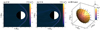 |
Fig. 4 Distribution of radial gradient of solar-wind velocity in (a) XY and (b) XZ planes for Case 2, with dashed lines representing the average bow-shock location (Vignes et al. 2000). (c) Martian bow-shock layer is color-coded based on the magnitude of solar-wind velocity, and it overlaps its vectors for Case 2. |
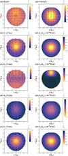 |
Fig. 5 Distribution of (a1) total magnetic-field magnitude and (a2) total current-density magnitude at the Martian bow shock for Case 2, along with corresponding vectors. The distribution of (b1) total electric field overlapping with its uniform vectors and (b2) its energy-transfer rate between solar-wind protons at the Martian bow shock for Case 2. The distributions of (c1–c2) motional, (d1–d2) Hall, and (e1–e2) ambipolar electric fields at the bow-shock layer for Case 2, along with the associate energy-transfer rates, are presented in a format consistent with that used for the b1-b2 total electric field. |
3.3 The influence of IMF By Strength
When the upstream IMF By doubles, the Martian-induced magnetosphere tends to be strengthened, which in turn is capable of preventing the invasion of the solar-wind plasma with lower MM S at greater distances, pushing the bow-shock layer further away from the Martian surface as demonstrated in Figs. 6a, b. Specifically, the subsolar and terminator positions of the bow shock expand to approximately 1.7 RM and 3.0 RM separately. Based on the criteria of the maximum radially inward VS W gradient, Figure 6c presents the Martian bow-shock layer extracted from simulation Case 3, overlapping with the VS W vectors. It is obvious that the dayside bow-shock layer under the double IMF By condition is the most expanded, where the solar-wind flow tends to be decelerated and deflected.
In order to investigate the influence of the strength of the IMF By on the physical characteristics within the Martian bow-shock layer, Figure 7 provides the distributions of the magnetic field, current density, electric fields, and the corresponding energy-transfer rates on the bow-shock layer under the double-IMF By condition, as viewed from the Sun. When the upstream IMF By is doubled, the pile-up IMF around the subsolar bow-shock layer approximately doubles to 15 nT (Fig. 7a1), giving rise to an increase of the induced current density to ~60 nA/m2 (Fig. 7a2). This enhancement of the magnetic field and current density at the bow shock results in the increase of the outward EH (Fig. 7d1) and the corresponding energy transfer rate (EH · JH+, Fig. 7d2) to 0.6 V /km and −2 × 10⁻¹⁰ W / m3, respectively, around the subsolar area. Moreover, the intensification of the magnetic field at the bow-shock layer also leads to a doubling of EM to ~5.0 V /km around the ±ZMS E flanks (Fig. 7c1). Despite the doubling of the EM, the energy transfer from the solar wind through this type of electric field still constitutes the smallest proportion of 1%, which is ~−0.15 × 10⁻¹⁰ W / m3 concentrated at the +ZMS E pole. However, the magnitude of the outward EA and the associated energy-transfer rate (EA · JH+), respectively, decline to 1.5 V /km and −5 × 10⁻¹⁰ W / m3 around the subsolar position. This is ascribed to the fact that the location of the bow shock is farther from the Martian surface in Case 3, thereby leading to the reduction of the electron pressure within the expanded Martian magnetosheath as compared to Case 1. Therefore, it can be deduced that a stronger IMF By tends to increase the distance of the Martian-bow-shock layer from the Martian surface, as well as the magnitudes of the magnetic field, current density, EM, and EH at the bow-shock layer; however, it decreases the magnitude of EA at the bow shock. Besides this, a significant increase in the energy transfer via EH and a decrease in the energy transfer through EA are observed around the lower SZAs, indicating that the effect of the outward EH at the Martian bow shock is strengthened under conditions of an intensified cross-flow component of the IMF.
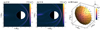 |
Fig. 6 Distribution of radial gradient of solar-wind velocity in (a) XY and (b) XZ planes for Case 3, with dashed lines representing the average bow-shock location (Vignes et al. 2000). (c) Martian bow-shock layer color-coded based on magnitude of solar-wind velocity and overlapping its vectors for Case 3. |
3.4 The influence of the IMF Parker spiral angle
In simulation Cases 1–3, the VS W and IMF are separately set in the −X and Y directions, indicating that the Parker spiral angle of the IMF is 90°. Under such solar-wind conditions, a dawn-dusk symmetrical quasi-perpendicular bow shock tends to be formed in front of the Martian obstacle. To explore the influence of the IMF Parker spiral angle on the physical properties at the Martian-bow-shock layer, we carried out simulation Case 4 with a Parker spiral angle of 56°, which represents the Mars-solar-wind interaction under the average upstream solar-wind condition. Figures 8a, b illustrate the distribution of the radial gradient of VS W in the XY and XZ planes, overlapping with solid white magnetic-field lines and dashed average-bow-shock locations, respectively. It is apparent from Fig. 8a that the magnetic-field lines are quasi-parallel to the normal direction of the bow shock within Y < 0, indicating that a portion of the quasi-parallel bow-shock layer tends to be formed when the IMF Parker spiral angle is not restricted to 90°. Employing the maximum value criterion of the radially inward gradient of VS W as previously mentioned, the bow-shock layer is extracted from simulation Case 4 as shown in Fig. 8c, where it is colored according to the magnitude of VS W and overlaps its vectors. The common features on the bow-shock layer can also be observed; namely, the solar-wind flow decelerates and deflects at the bow-shock layer.
To reveal the impact of the IMF Parker spiral angle on the characteristics of the magnetic field and current density at the bow-shock layer, Figs. 9a1–a4 and b1–b4 depict the corresponding distributions accompanied by associated components, overlapping their vectors separately, in circumstances where the IMF Parker spiral angle is 56°. It is evident from Figs. 9a1–a4 that the distributions of the magnetic field exhibit distinct asymmetries. Specifically, the total magnetic field is stronger at the +Y bow-shock layer due to the fact that the Bx and By at the +Y bow-shock layer are 1 ~ 2 nT greater than the corresponding ones at the −Y layer, indicating that the IMFs are more inclined to drape and pile up at the quasi-perpendicular bow shock. While Bz is more intense at the −Y bow shock layer, implying that IMFs are more prone to slip at the quasi-parallel bow shock. Meanwhile, the asymmetry of the magnetic field gives rise to the asymmetrical distribution of the current density, as illustrated in Figs. 9b1–b4. The more intense Bx and By at the quasi-perpendicular bow shock induce stronger Jz (~30 nA/m2) at the corresponding location (+Y layer), resulting in the shift of the strongest total current density to the quasi-perpendicular bow-shock layer as compared with Case 1. Besides this, the positive Bz and negative Bx around the +Z bow shock, as well as the negative Bz and Bx around the −Z bow shock, respectively, give rise to positive Jy (~5 nA/m2) around the +Z bow shock and negative Jy (~−5 nA/m2) around the −Z bow shock, thereby bending the current flow within the bow-shock layer. Accordingly, if the IMF Parker spiral angle is not limited to 90°, a portion of the Martian quasi-perpendicular bow-shock layer will transform into quasi-parallel shock, where IMFs struggle to pile up but are prone to slipping. Subsequently, the strongest total magnetic field and the associated current density tend to shift from the subsolar position to the quasi-perpendicular bow shock, and the current flow bends surrounding the quasi-parallel bow shock.
Figure 10 presents the distributions of electric fields and associated energy-transfer rates between the solar wind plasma used to investigate the influence of the IMF Parker spiral angle on these physical characteristics at the Martian bow shock. Owing to the stronger magnetic field and current density existing at the +Y bow-shock layer, stronger EH (~0.15 V /km) with outward directions and the associated energy-transfer rate (EH · JH+ ~−0.5 × 10⁻¹⁰ W / m3) also emerge there, as shown in Figs. 10c1–c2. According to EM = −VS W × B, the magnitude of EM will diminish if VS W and B remain invariant, but the angle between them is no longer equal to 90°. Therefore, in contrast to Case 1, the EM around the ±ZMS E flanks at the bow shock decreases to 2.0 V /km, and the corresponding energy-transfer rates around the +ZMS E pole decrease to −0.1 × 10⁻¹⁰ W / m3 (Figs. 10b1–b2). However, the dominant outward EA and the associated energy-transfer rate remain almost unchanged compared with Case 1, with the magnitudes reaching 2.5 V /km and −10 × 10−10 W / m3 separately around the subsolar area; this is mainly attributed to the similar locations of the bow-shock layer derived from these two simulation cases.
In conclusion, if the IMF Parker spiral angle is not confined to 90°, a portion of the Martian bow shock exhibits the characteristics of a quasi-parallel shock, where the magnetic field, current density, EH, and the associated energy-transfer rate between the solar-wind flows (EH · JH+) are smaller than those at the corresponding quasi-perpendicular shock. Moreover, the total electric field and the associated energy-transfer rate become lower around the +ZMS E pole as a result of the decrease in EM and remain almost unchanged around the lower SZAs due to the fact that the dominant EA is almost invariant there.
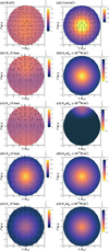 |
Fig. 7 Distribution of (a1) total magnetic-field magnitude and (a2) total current-density magnitude at the Martian bow shock for Case 3, along with corresponding vectors. The distribution of (b1) total electric field overlapping its uniform vectors and (b2) its energy-transfer rate between solar-wind protons at the Martian bow shock for Case 3. The distributions of (c1–c2) motional, (d1–d2) Hall, and (e1–e2) ambipolar electric fields at the bow-shock layer for Case 3, along with the associated energy-transfer rates, are presented in a format consistent with that used for the b1-b2 total electric field. |
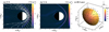 |
Fig. 8 Distribution of radial gradient of solar-wind velocity in (a) XY and (b) XZ planes for Case 4, overlapping the solid magnetic-field lines and dashed average bow shock locations (Vignes et al. 2000) separately. (c) Martian bow-shock layer color-coded based on magnitude of solar-wind velocity and overlapping its vectors for Case 4. |
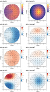 |
Fig. 9 Distribution of (a1) total magnetic-field magnitude and (a2, a3, a4) its components (Bx, By, Bz) at the Martian bow-shock layer for Case 4 overlapping magnetic field vectors. The distribution of the (b1) total current-density magnitude and (b2, b3, b4) its components (Jx, Jy, Jz) at the bow-shock layer for Case 4 overlapping current vectors. |
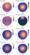 |
Fig. 10 Distribution of (a1) total electric field overlapping its uniform vectors and (a2) its energy-transfer rate between solar-wind protons at the Martian bow shock for Case 4. The distributions of (b1–b2) motional, (c1–c2) Hall, and (d1–d2) ambipolar electric fields at the bow-shock layer for Case 4, along with the associated energy-transfer rates, are presented in a format consistent with that used for the a1–a2 total electric field. |
4 Conclusions
By taking advantage of the multi-fluid Hall-MHD model and employing the maximum radially inward gradient of the VS W to extract the bow-shock layer, this study reveals comprehensive distributions of physical characteristics within the Martian-bow-shock layer, including the magnetic field, current density, electric fields, and the corresponding energy-transfer rates between the fields and solar-wind protons. Furthermore, this study also explores the influence of external solar-wind drivers on these physical characteristics at the bow-shock layer, such as the magnitude of the VS W and the magnitude and Parker spiral angle of the IMF.
Under normal conditions with an IMF Parker spiral angle of 90°, the associated simulation results indicate that the IMFs display symmetrical yet complex behaviors at the Martian bow-shock layer, such as pile-up around the subsolar area, draping and bending on the ±YMS E layer, and slipping around the ±ZMS E poles. Such symmetrical magnetic-field topology at the Martian bow shock tends to induce currents in the −ZMS E – direction flowing from the +ZMS E flank toward the −ZMS E flank – with the strongest magnitude around the subsolar locations. The ET at the Martian bow-shock layer is composed of the EM in the +ZMS E direction around the ±ZMS E flanks and the outward EA around the lower SZAs, along with the minimal contribution of the outward EH around the subsolar area. According to the energy-transfer rates between the electromagnetic fields and the solar-wind protons, it can be deduced that the solar wind is prone to losing most of its energy through the EA.
When the upstream VS W doubles, the Martian bow shock is compressed during the Mars-solar-wind interaction, resulting in stronger magnetic fields, current density, electric fields, and the corresponding energy transfer from the solar-wind protons at the bow-shock layer. When the magnitude of the upstream cross-flow IMF component (By) doubles, the Martian bow shock expands as a result of the stronger Martian-induced magnetosphere. This expanded bow-shock layer exhibits a stronger magnetic field, current density, EM, and EH, but a weaker EA. Therefore, the solar wind tends to transfer its kinetic energy to the Martian electromagnetic fields predominantly through the EA and EH, indicating that the effect of the EH is significantly enhanced under larger IMF conditions. When the upstream Parker spiral angle of the IMF is not restricted to 90°, a portion of the quasi-parallel bow-shock layer is formed, giving rise to asymmetrical physical characteristics at the Martian bow-shock layer. More specifically, when the upstream IMF Parker spiral angle is 56°, the magnetic fields are more prone to slip, making it difficult to pile up at the quasi-parallel bow-shock layer compared to those of the corresponding quasi-perpendicular bow shock. This leads to the curvature of the associated current density surrounding the quasi-parallel bow shock, as well as stronger EH and an associated energy-transfer rate at the quasi-perpendicular bow shock. However, under this solar wind condition, the dominant electric fields at the Martian bow shock are also the outward EA distributed around the lower SZAs and EM with the +ZMS E direction at the ±ZMS E flanks, through which the solar-wind plasma transfers its kinetic energy to the Martian electromagnetic fields.
This study is dedicated to uncovering the physical features at the Martian bow shock and highlighting the influence exerted by the external drivers of the solar wind on these physical characteristics. However, certain internal influencing factors, such as the Martian ionosphere, which can be affected by the solar extreme ultraviolet radiation and the crustal magnetic fields (Gruesbeck et al. 2018; Garnier et al. 2022b), can also exert impacts on the location and shape of the Martian-bow-shock layer as well as associated physical characteristics, thus warranting further investigations in the near future.
Acknowledgements
This work was supported by the National Natural Science Foundation of China under Grants 42241114, 42330207, 42074214, 12150008 and 42404176, the B-type Strategic Priority Program of the Chinese Academy of Sciences (Grant XDB41000000), the Postdoctoral Fellowship Program of CPSF under Grant GZC20233367.
References
- Acuna, M., Connerney, J., Ness, et al. 1999, Science, 284, 790 [NASA ADS] [CrossRef] [Google Scholar]
- Boscoboinik, G., Bertucci, C., Gomez, D., et al. 2023, Icarus, 401, 115598 [Google Scholar]
- Bougher, S. W., Engel, S., Hinson, D. P., & Forbes, J. M. 2001, GRL, 28, 3091 [Google Scholar]
- Chai, L., Wan, W., Wei, Y., et al. 2019, ApJ, 871, L27 [Google Scholar]
- Connerney, J. E., Espley, J. R., DiBraccio, G. A., et al. 2015, GRL, 42, 8819 [Google Scholar]
- Dong, H.-T., Zhang, L.-D., & Lee, C.-H. 2002, CFDJ, 10, 563 [Google Scholar]
- Dong, C., Bougher, S. W., Ma, Y., et al. 2014, GRL, 41, 2708 [NASA ADS] [CrossRef] [Google Scholar]
- Dong, C., Bougher, S. W., Ma, Y., et al. 2015, JGRA, 120, 7857 [Google Scholar]
- Dubinin, E., Fränz, M., Woch, J., et al. 2006, SSRv, 126, 209 [Google Scholar]
- Dubinin, E., Modolo, R., Fraenz, M., et al. 2019, GRL, 46, 12722 [Google Scholar]
- Edberg, N., Lester, M., Cowley, S., & Eriksson, A. 2008, JGRA, 113 [Google Scholar]
- Edberg, N. J. T., Brain, D. A., Lester, M., et al. 2009, AnGeo, 27 [Google Scholar]
- Fang, X., Ma, Y., Brain, D., Dong, Y., & Lillis, R. 2015, JGRA, 120, 10 [Google Scholar]
- Garnier, P., Jacquey, C., Gendre, X., et al. 2022a, JGRA, 127, e2021JA030147 [Google Scholar]
- Garnier, P., Jacquey, C., Gendre, X., et al. 2022b, J. Geophys. Res.: Space Phys., 127, e2021JA030146 [Google Scholar]
- Gruesbeck, J. R., Espley, J. R., Connerney, J. E., et al. 2018, JGRA, 123, 4542 [Google Scholar]
- Halekas, J., Ruhunusiri, S., Harada, Y., et al. 2017, JGRA, 122, 547 [Google Scholar]
- Hall, B. E. S., Lester, M., Sánchez-Cano, B., et al. 2016, JGRA, 121, 11 [Google Scholar]
- Huestis, D. L. 2001, JQSRT, 69, 709 [Google Scholar]
- Jakosky, B. M., Grebowsky, J. M., Luhmann, J. G., & Brain, D. A. 2015, GRL, 42, 8791 [Google Scholar]
- Li, S., Lu, H., Cui, J., et al. 2020, EPP, 4, 23 [Google Scholar]
- Li, S., Lu, H., Cao, J., et al. 2022a, ApJ, 941, 198 [NASA ADS] [CrossRef] [Google Scholar]
- Li, S., Lu, H., Cao, J., et al. 2022b, ApJ, 931, 30 [Google Scholar]
- Li, S., Lu, H., Cao, J., et al. 2023, ApJ, 949, 88 [Google Scholar]
- Li, S., Lu, H., Cao, J., et al. 2024a, GRL, 51, e2024GL109186 [Google Scholar]
- Li, S., Lu, H., Cao, J., et al. 2024b, GRL, 51, e2024GL110646 [Google Scholar]
- Li, S., Wang, S., Lu, H., et al. 2025, GRL, 52, e2024GL113340 [Google Scholar]
- Ma, Y., Dong, C., Toth, G., et al. 2019, J. Geophys. Res.: Space Phys., 124, 9040 [Google Scholar]
- MacCormack, R. W. 2003, JSR, 40, 757 [Google Scholar]
- Mazelle, C., Winterhalter, D., Sauer, K., et al. 2004, SSRv, 111, 115 [Google Scholar]
- Najib, D., Nagy, A. F., Tóth, G., & Ma, Y. 2011, JGRA, 116 [Google Scholar]
- Ramstad, R., Barabash, S., Futaana, Y., & Holmström, M. 2017, JGRA, 122, 7279 [Google Scholar]
- Ramstad, R., Brain, D. A., Dong, Y., et al. 2020, NatAs, 4, 979 [Google Scholar]
- Riedler, W., Möhlmann, D., Oraevsky, V., et al. 1989, Nature, 341, 604 [NASA ADS] [CrossRef] [Google Scholar]
- Russell, C. 1977, GRL, 4, 387 [Google Scholar]
- Russell, C. 1978a, GRL, 5, 81 [Google Scholar]
- Russell, C. 1978b, GRL, 5, 85 [Google Scholar]
- Schunk, R. W., & Nagy, A. F. 2009, Ionospheres: Physics, Plasma Physics, and Chemistry (Cambridge University Press) [CrossRef] [Google Scholar]
- Smith, E. J., Davis Jr, L., Coleman Jr, P. J., & Jones, D. E. 1965, Science, 149, 1241 [Google Scholar]
- Song, Y., Lu, H., Cao, J., et al. 2023a, JGRA, 128, e2022JA031083 [NASA ADS] [Google Scholar]
- Song, Y., Lu, H., Cao, J., et al. 2023b, JGRA, 128, e2023JA031788 [NASA ADS] [Google Scholar]
- Song, Y., Lu, H., Cao, J., et al. 2025, JGRE, 130, e2024JE008603 [Google Scholar]
- Sui, H., Wang, M., Lu, J., Zhou, Y., & Wang, J. 2023, ApJ, 945, 136 [Google Scholar]
- Trotignon, J. G., Grard, R., & Klimov, S. 1991a, GRL, 18, 365 [Google Scholar]
- Trotignon, J. G., Grard, R., & Savin, S. 1991b, JGRA, 96, 11253 [Google Scholar]
- Trotignon, J., Grard, R., & Skalsky, A. 1993, PSS, 41, 189 [Google Scholar]
- Trotignon, J., Mazelle, C., Bertucci, C., & Acuña, M. 2006, PSS, 54, 357 [Google Scholar]
- Vignes, D., Mazelle, C., Rme, H., et al. 2000, GRL, 27, 49 [Google Scholar]
- Wang, M., Xie, L., Lee, L., et al. 2020, ApJ, 903, 125 [Google Scholar]
- Wang, X.-D., Fatemi, S., Nilsson, H., et al. 2023, MNRAS, 521, 3597 [Google Scholar]
- Wang, X.-D., Fatemi, S., Holmström, M., et al. 2024, MNRAS, 527, 12232 [Google Scholar]
- Xu, S., Mitchell, D. L., Ma, Y., et al. 2021, JGRA, 126, e2021JA029764 [Google Scholar]
- Yuan, Y., Wang, M., Lu, J., Chen, J., & Cheng, N. 2024, ApJ, 976, 245 [Google Scholar]
- Zhang, T. L., Schwingenschuh, K., Lichtenegger, H., et al. 1991, JGRA, 96, 11265 [Google Scholar]
All Tables
Settings of upstream solar-wind velocity (VS W) and interplanetary magnetic field (IMF) as well as corresponding magnetosonic Mach number (MM S) in the simulation cases.
All Figures
|
Fig. 1 Distribution of solar-wind velocity in (a) XY and (c) XZ planes for Case 1, overlapping with its vectors. The distribution of the radial gradient of the solar-wind velocity in the (b) XY and (d) XZ planes for Case 1 is shown overlapping with dashed average bow-shock locations (Vignes et al. 2000). (e) Martian-bow-shock layer colored based on the magnitude of the solar-wind velocity and overlapping with its vectors for Case 1. (f) Locations of XMS E at Martian-bow-shock layer for Case 1 along with three corresponding contoured solid lines, as viewed from the Sun. |
| In the text | |
|
Fig. 2 Distribution of (a1) total magnetic-field magnitude and (a2, a3, a4) its components (Bx, By, Bz) at the Martian bow-shock layer for Case 1, overlapping with magnetic-field vectors. The distribution of (b1) total current density magnitude and (b2, b3, b4) its components (Jx, Jy, Jz) at the bow-shock layer for Case 1, overlapping with current vectors. |
| In the text | |
|
Fig. 3 Distribution of (a1) total electric-field overlapping with its uniform vectors and (a2) its energy-transfer rate between solar-wind protons at the Martian bow shock for Case 1. The distributions of (b1–b2) motional, (c1–c2) Hall, and (d1–d2) ambipolar electric fields at the bow-shock layer for Case 1, along with the associated energy transfer rates, are presented in a format consistent with that used for the a1–a2 total electric-field. |
| In the text | |
|
Fig. 4 Distribution of radial gradient of solar-wind velocity in (a) XY and (b) XZ planes for Case 2, with dashed lines representing the average bow-shock location (Vignes et al. 2000). (c) Martian bow-shock layer is color-coded based on the magnitude of solar-wind velocity, and it overlaps its vectors for Case 2. |
| In the text | |
|
Fig. 5 Distribution of (a1) total magnetic-field magnitude and (a2) total current-density magnitude at the Martian bow shock for Case 2, along with corresponding vectors. The distribution of (b1) total electric field overlapping with its uniform vectors and (b2) its energy-transfer rate between solar-wind protons at the Martian bow shock for Case 2. The distributions of (c1–c2) motional, (d1–d2) Hall, and (e1–e2) ambipolar electric fields at the bow-shock layer for Case 2, along with the associate energy-transfer rates, are presented in a format consistent with that used for the b1-b2 total electric field. |
| In the text | |
|
Fig. 6 Distribution of radial gradient of solar-wind velocity in (a) XY and (b) XZ planes for Case 3, with dashed lines representing the average bow-shock location (Vignes et al. 2000). (c) Martian bow-shock layer color-coded based on magnitude of solar-wind velocity and overlapping its vectors for Case 3. |
| In the text | |
|
Fig. 7 Distribution of (a1) total magnetic-field magnitude and (a2) total current-density magnitude at the Martian bow shock for Case 3, along with corresponding vectors. The distribution of (b1) total electric field overlapping its uniform vectors and (b2) its energy-transfer rate between solar-wind protons at the Martian bow shock for Case 3. The distributions of (c1–c2) motional, (d1–d2) Hall, and (e1–e2) ambipolar electric fields at the bow-shock layer for Case 3, along with the associated energy-transfer rates, are presented in a format consistent with that used for the b1-b2 total electric field. |
| In the text | |
|
Fig. 8 Distribution of radial gradient of solar-wind velocity in (a) XY and (b) XZ planes for Case 4, overlapping the solid magnetic-field lines and dashed average bow shock locations (Vignes et al. 2000) separately. (c) Martian bow-shock layer color-coded based on magnitude of solar-wind velocity and overlapping its vectors for Case 4. |
| In the text | |
|
Fig. 9 Distribution of (a1) total magnetic-field magnitude and (a2, a3, a4) its components (Bx, By, Bz) at the Martian bow-shock layer for Case 4 overlapping magnetic field vectors. The distribution of the (b1) total current-density magnitude and (b2, b3, b4) its components (Jx, Jy, Jz) at the bow-shock layer for Case 4 overlapping current vectors. |
| In the text | |
|
Fig. 10 Distribution of (a1) total electric field overlapping its uniform vectors and (a2) its energy-transfer rate between solar-wind protons at the Martian bow shock for Case 4. The distributions of (b1–b2) motional, (c1–c2) Hall, and (d1–d2) ambipolar electric fields at the bow-shock layer for Case 4, along with the associated energy-transfer rates, are presented in a format consistent with that used for the a1–a2 total electric field. |
| In the text | |
Current usage metrics show cumulative count of Article Views (full-text article views including HTML views, PDF and ePub downloads, according to the available data) and Abstracts Views on Vision4Press platform.
Data correspond to usage on the plateform after 2015. The current usage metrics is available 48-96 hours after online publication and is updated daily on week days.
Initial download of the metrics may take a while.