| Issue |
A&A
Volume 694, February 2025
|
|
|---|---|---|
| Article Number | A189 | |
| Number of page(s) | 10 | |
| Section | Planets, planetary systems, and small bodies | |
| DOI | https://doi.org/10.1051/0004-6361/202453085 | |
| Published online | 12 February 2025 | |
The impact of interplanetary magnetic field intensity on the Martian ionosphere
1
School of Space and Earth Sciences, Beihang University,
Beijing,
China
2
Key Laboratory of Space Environment Monitoring and Information Processing, Ministry of Industry and Information Technology,
Beijing,
China
★ Corresponding author; This email address is being protected from spambots. You need JavaScript enabled to view it.
Received:
20
November
2024
Accepted:
17
January
2025
Abstract
Context. The interplanetary magnetic field (IMF) is one of the important external drivers that controls the Martian-induced magnetosphere and ionosphere. Previous studies have shown that the ion escape process is highly influenced by both the direction and intensity of the IMF. The enhanced IMF may decrease the ion escape rate by inducing a stronger magnetosphere that protects the Martian ionosphere, but the mechanisms have not been investigated thoroughly. Further studies are needed to reveal the response of ionospheric heavy ions to IMF variation as well as the underlying physical mechanism.
Aims. This study aims to investigate the influence the IMF strength has on the Martian ionosphere. We adopted a multifluid magnetohydrodynamic model in this study, which can self-consistently simulate the interaction between solar wind and Mars. By comparing different cases, we analyzed the ionospheric structure on the dayside and near nightside as well as the ion transport process. We aim to obtain a deeper understanding of how the IMF intensity variation impacts the Martian ionosphere and the escape of planetary ions.
Methods. A three-dimensional multifluid MHD model was used to simulate the interaction between the upstream solar wind and Mars. Four major species in the Martian ionosphere, H+, O2+, O+, and CO2+, are considered in the model, with the chemical reactions and particle collisions included to calculate ion distribution and ion motions. We analyzed three cases where the IMF strength was set to 1 nT, 3 nT, and 5 nT.
Results. The enhancement of the IMF produces a stronger electromagnetic field in the Martian plasma environment. Both the electric field and magnetic field intensity increase, which provides a shielding effect to the Martian ionosphere, hindering the intrusion of solar wind particles. Thus, less planetary ions are produced by the chemical reactions between the solar wind and the Martian neutral particles, leading to shrinkage of the ionospheric upper boundary. As the IMF strength increases, both the day-to-night plasma transport and the ion outflow decreases. Thus, a more depleted nightside ionosphere is formed, and the tailward ion escape may be weakened, decreasing the global ion escape rate. Moreover, the strong crustal fields in the southern hemisphere enhance the electromagnetic field on the southern dayside, which withstand the penetration of solar wind plasma more effectively, resulting in asymmetry structures in the ionosphere.
Key words: magnetohydrodynamics (MHD) / methods: numerical / planets and satellites: terrestrial planets
© The Authors 2025
 Open Access article, published by EDP Sciences, under the terms of the Creative Commons Attribution License (https://creativecommons.org/licenses/by/4.0), which permits unrestricted use, distribution, and reproduction in any medium, provided the original work is properly cited.
This article is published in open access under the Subscribe to Open model. This email address is being protected from spambots. You need JavaScript enabled to view it. to support open access publication.
1 Introduction
It is widely believed that ~3.5 Gyr years ago ancient Mars possessed a denser atmosphere, and therefore, the early climate of Mars may have been warm and humid enough to sustain surface water and potentially able to host life (e.g., Jakosky et al. 2017; McKay & Stoker 1989; Wordsworth 2016). However, the atmosphere of Mars experienced a significant loss from then on, with the Martian atmospheric pressure decreasing from ~0.1 bar to ~6 mbar in the present (Jakosky & Phillips 2001). The nonthermal atmospheric escape process is one of the important pathways for Martian atmospheric loss since the end of the Noachian Period (e.g., Lammer et al. 2013; Shizgal & Arkos 1996). Therefore, investigating the influence of solar wind conditions, solar extreme ultraviolet (EUV), and crustal field on atmospheric escape is beneficial for picturing the outgassing history of the Martian atmosphere.
Unlike Earth or Jupiter, Mars does not possess a global intrinsic magnetic field. The solar wind interacts directly with the upper atmosphere of Mars to form the induced magnetosphere and magnetotail (e.g., Cui et al. 2020; Kallio et al. 2008; Matsunaga et al. 2017; Ramstad et al. 2020), and local crustal magnetic fields that are distributed mainly in the southern hemisphere have been reported (Acuña et al. 1998; Acuna et al. 1999). The existence of local crustal fields modifies the morphology of the magnetic field, thus playing an important role in controlling the plasma distribution on Mars. The crustal field can cause the formation of a mini-magnetosphere and uplift the magnetospheric pileup boundary (MPB) and bow shock (BS) (e.g. Breus et al. 2005; Edberg et al. 2008; Fan et al. 2023; Fang et al. 2017; Garnier et al. 2022; Harnett & Winglee 2003; Song et al. 2023b). Previous studies have shown that local crustal fields in the southern hemisphere hinder parallel ion transport while facilitating vertical ion transport, causing asymmetrical features in the dayside and near-nightside ionosphere (e.g., Girazian et al. 2017a; Li et al. 2022a,b; Song et al. 2023b).
The Martian ionosphere has been a subject of study since the first Martian mission (e.g., Chen et al. 1978; Gurnett et al. 2008; Vogt et al. 2015). The primary plasma source in the dayside ionosphere is the photoionization process. On the nightside, day-to-night plasma transport and electron precipitation dominate (Withers 2009; Zhang et al. 1990), forming a patchy and sporadic nightside ionosphere. The main peaks in the nightside ionosphere occur between 120 and 180 km, with the peak electron density approximately one to two orders of magnitude lower than the dayside peak density (e.g., Fowler et al. 2015; Girazian et al. 2017b; Lillis et al. 2009). The trans-terminator plasma transport, which is strongly dependent on the dayside ionospheric structure and the upstream solar wind conditions, functions as a main plasma source in the nightside with SZA<115° (Cao et al. 2019; Chaufray et al. 2014; Cui et al. 2015; Withers et al. 2012; Song et al. 2023b). The occurrence rate of the nightside ionosphere decreases with increasing SZA, indicating that the influence of plasma transport on the nightside ionosphere does not terminate until SZA = 125° (Němec et al. 2010). In the deep nightside ionosphere (SZA>115°), the electron precipitation controls the plasma source.
External drivers such as solar wind dynamic pressure, solar irradiation, and the interplanetary magnetic field (IMF) can profoundly influence the Martian ionosphere and ion escape (Edberg et al. 2009). The variation in the IMF is one of the important features of solar wind events. During interplanetary coronal mass ejection and co-rotating interaction region events, the IMF strength is significantly enhanced, and the IMF direction as well as the magnetic topology vary significantly, thus affecting the plasma transport process (e.g., Dong et al. 2015; Ma et al. 2017; Sakai et al. 2021; Xu et al. 2018, 2019). The upper ionosphere is strongly asymmetric in the direction of the upstream motional electric field −VS W × BI M F, which is highly influenced by the direction and intensity of the IMF (e.g., Dubinin et al. 2018, 2019). At higher values of the cross-flow component of the IMF, the dayside ionosphere shrinks, while in the E+ hemisphere (ZM S E>0) the ionosphere expands to a higher altitude than in the E− hemisphere (ZM S E<0). Fowler et al. (2022) observed a severely eroded dayside ionosphere in a case study with radial IMF, with both the altitudes of the upper ionosphere and the ionospheric densities significantly reduced compared to the average conditions. Diéval et al. (2014) also reported the impact of IMF direction on the nightside ionosphere, showing that very high nightside ionospheric peak densities are often associated with the westward IMF. Moreover, ion escape is also controlled by the direction and strength of the IMF. The Martian ion escape rate is much lower in the northward (parallel) IMF compared to the southward (antiparallel) IMF, with the escape rate increasing from ~5 × 10²³ s−1 to ~3 × 1025 s−1 during the IMF rotation from parallel to the intrinsic magnetic field to antiparallel (Sakai et al. 2021, 2023). Using a hybrid simulation model, Zhang et al. (2023) studied the influence of the IMF intensity and direction on the heavy ion escape rate. Their simulation results show that the enhancement of the IMF can result in a stronger induced magnetosphere, which then leads to a decrease of the heavy ion escape rate, but the detailed mechanisms of these processes have not been analyzed thoroughly. In general, previous studies have focused mainly on the influence of IMF directions instead of IMF intensity. In addition, the response of the Martian ionosphere to the variation of the IMF strength has not been analyzed systematically, meaning the underlying mechanisms still need to be revealed.
In solar wind events, external drivers such as solar wind dynamic pressure, solar EUV, and IMF conditions all vary simultaneously. The mixed effects caused by multiple factors complicate the scenario, making it challenging to distinguish the influence of IMF strength on the Martian ionosphere. The in situ observational data are also limited by satellite orbits and the temporal sampling coverage. Thus, to investigate the Martian ionosphere response to the IMF intensity variation while revealing the physical mechanism, a study based on the global simulation model is necessary.
There are three main approaches to simulating the Solar System plasmas and the interactions with planets: the gas-dynamic model, the hybrid model, and the magnetohydrodynamic (MHD) model (Ledvina et al. 2017). In this study, a 3D multifluid MHD model is applied to simulate the interaction between solar wind and Mars, and in the model the mass, momentum, and energy equations are solved separately for each fluid component. In our previous studies, the impact of solar wind dynamic pressure, including individual variation of solar wind density and velocity, on the Martian ionosphere and magnetosphere was investigated, which validates the reliability of our model. As the IMF is also one of the important external drivers that controls the Martian plasma environment, we focus on the influence of IMF intensity on the Martian ionosphere. Three cases with ideal solar wind parameters are analyzed in this work. We first compare the nightside electron density profiles under different IMF intensities, and then the plasma transport and ion distribution at ionospheric altitudes (100–600 km) are analyzed, revealing the possible mechanisms in the changes of ionospheric structures. The rest of the paper is organized as follows: A detailed model description is presented in Section 2, simulation results are shown in Section 3, and Section 4 provides the conclusion of our study.
2 Model description
In this study, a 3D multifluid MHD model that has been utilized and validated in numerous previous researches is applied to simulate the Martian ionosphere and magnetosphere (e.g., Li et al. 2022a,b). Four major ion species in the Martian ionosphere are included: ![Mathematical equation: $\[\mathrm{H}^{+}, \mathrm{O}_{2}^{+}, \mathrm{O}^{+}\]$](/articles/aa/full_html/2025/02/aa53085-24/aa53085-24-eq3.png) , and
, and ![Mathematical equation: $\[\mathrm{CO}_{2}^{+}\]$](/articles/aa/full_html/2025/02/aa53085-24/aa53085-24-eq4.png) . The ion species are self-consistently produced through ionospheric chemical reactions, including photoionization, charge exchange, and recombination reactions (Ma et al. 2004; Najib et al. 2011; Li et al. 2020). The ion transport processes are also considered in the model, increasing the accuracy of the dayside and near-nightside ionosphere simulation (Song et al. 2023b).
. The ion species are self-consistently produced through ionospheric chemical reactions, including photoionization, charge exchange, and recombination reactions (Ma et al. 2004; Najib et al. 2011; Li et al. 2020). The ion transport processes are also considered in the model, increasing the accuracy of the dayside and near-nightside ionosphere simulation (Song et al. 2023b).
In this model, a one-dimensional neutral density profile derived from Bougher et al. (2000) is adopted so that the oxygen corona is incorporated. We chose three neutral species, CO2, O, and H, which are the main neutral components of the Martian atmosphere. The Chapman function instead of a simple cosine function of the solar zenith angle (SZA) was employed to calculate the optical depth effects, allowing for more accurate modeling of the Martian ionosphere, especially in simulation of the M2 layer. The multifluid MHD model solves the continuity, momentum, and energy equations independently for each ion species as well as a magnetic induction equation that includes the Hall term and thermal pressure gradient term. Inelastic collisions (charge exchange, recombination, and photoionization) and elastic collisions (ion-neutral and ion-ion collisions) were considered in the source term of the MHD equations. A detailed description of the MHD model can be found in Song et al. (2023a).
The simulation was conducted under the Mars-centered Solar Orbital (MSO) coordinate system, in which the X-axis points from Mars to the Sun, the Z-axis is parallel to the north celestial pole, and the Y-axis completes the right-handed coordinate system. The computational domain was set to −24 RM ≤ X ≤ 8 RM, −16 RM ≤ Y ≤ 16 RM, and −16 RM ≤ Z ≤ 16 RM, where RM represents the average radius of Mars (RM ≈ 3396 km). The simulation grid consists of 960 000 cells, with the minimum radial grid size set to 10 km at the inner boundary of 100 km above the Martian surface. In our model, only one H+ population is considered, and solar wind protons and planetary protons are not distinguished. Therefore, at the inner boundary, the density and velocity of H+ are assumed to be 0.3 of the solar wind density and zero, while the ion densities are assumed to be the photochemical equilibrium, based on the work of Dong et al. (2014). The simulation assumes a solar irradiance condition at solar maximum. The remnant crustal field is simulated by using the 110° spherical harmonic crustal field model developed by Gao et al. (2021), with the strongest crustal field located on the dayside.
According to the statistical solar wind parameters upstream of Mars (Liu et al. 2021), three simulation cases with varying IMF strength were studied, as detailed in Table 1. The solar wind velocity was aligned with the X-axis in the MSO coordinate system. The IMF direction was set at a 56° Parker spiral angle in the X − Y plane; as an example, the IMF vector for Case 2 is (−1.68, 2.49, 0) nT in the MSO coordinate system.
Upstream solar wind condition settings of simulation cases.
3 Simulation results
We initially investigated the ion density distributions of the dayside and near-nightside ionosphere for different IMF conditions. The mean electron density (ne) profiles at ionospheric altitudes are depicted in Figure 1. Here, we present data with SZA ranges from 80° to 120°, for the day-to-night plasma transport dominates the plasma source in the near-nightside ionosphere (SZA<115°). At higher solar zenith angles, the nightside ionosphere is mainly produced by electron precipitation (Cui et al. 2015; Qin et al. 2022; Withers et al. 2012), which is not included in our model.
As shown in Figure 1, the electron density peaks are located between 150 and 200 km in the terminator and near-nightside regions, with the peak values decreasing with increasing SZA, which coincides with previous observational studies (Fowler et al. 2015; Girazian et al. 2017b; Qin et al. 2022). For the |IMF| = 3 nT case, which is taken as the normal condition case, the peak density decreases from 104.5 e−/cm3 in the SZA range of 80°–90° to 103.2 e−/cm3 in the SZA range of 110°–120°. The electron density displays a clear decrease with increasing IMF intensity. Near the terminator with the SZA range of 80°–100°, the expansion of electron density profiles only appears at the upper ionosphere, where the altitude is larger than 400 km. For the near-nightside region with the SZA range of 100°–120°, the inflation of density profiles occurs at all altitudes above 110 km. It is apparent that from the terminator to the near-nightside ionosphere, the response of electron density to IMF variation becomes more significant. In the SZA region of 110°–120°, the peak electron density depletes from 103.5 to 103 e−/cm3 as the IMF strength increases from 1 to 5 nT, while in the SZA region of 80°–90°, the peak density is almost the same for all three cases. Therefore, it is reasonable to deduce that the day-to-night plasma transport process is considerably influenced by changes in IMF strength since the near-nightside ionosphere is controlled by plasma transport. The discrepancy in electron density between the northern and southern hemispheres occurs mainly above 300 km. In the SZA range of 80°–90°, the electron density in the upper ionosphere is larger in the southern hemisphere compared to the northern one, while in the SZA range of 100°–120°, the near-nightside ionosphere is denser in the north. This north-south asymmetry could be explained by the hindering effect of the strong crustal field in the southern hemisphere on the horizontal plasma transport process.
Figure 2 shows the mean electron density distribution and the upper ionospheric boundary for different IMF intensity conditions. The data set has been divided into the northern hemisphere and the southern hemisphere, illustrating both the influence of IMF strength and the crustal magnetic field. The plots correspond to the SZA range of 0°–120° with a bin-size of 5° and to the altitude range of 120–600 km with a bin-size of 20 km. The ionospheric upper boundary, which is defined by the isoelectron density lines for ne = 100 cm−3, is marked by white lines to indicate how far the ionosphere extends (Ma et al. 2014). We note that the ionospheric upper boundary presented here is not the ionopause, which is usually identified by a sudden drop in electron density with increasing altitude in the Martian ionosphere or by the pressure balance criteria (Sánchez-Cano et al. 2020). Since the Martian ionosphere is sporadic and was not continuously observed, especially on the nightside (Duru et al. 2009, 2020; Vogt et al. 2015), we chose the artificially defined upper boundary instead of the ionopause to demonstrate the expansion and shrinkage of the ionosphere.
As shown in Figures 2a,b, in the Martian dayside, the ionospheric upper boundary is clearly uplifted in the southern hemisphere compared to the northern one, which is consistent with previous observational studies (e.g., Andrews et al. 2023; Chu et al. 2019; Dubinin et al. 2019; Flynn et al. 2017; Withers 2009). While in the near nightside, confirming the result in Figure 1, the upper boundary in the southern hemisphere is slightly lower than that in the north, but the difference is not significant.
In panels c and d, the upper boundary of the dayside ionosphere is located at an altitude range of 400–500 km in the northern hemisphere, while in the southern hemisphere, the upper boundary appears at a 450–550 km range. The simulated upper boundary coincides well with the observed altitude where ne = 100 cm−3 (Morgan et al. 2008), confirming the validation of our model. With increasing |IMF|, the ionospheric upper boundary appears to shrink in both hemispheres. The plasma transport process only changes the distribution of ions and electrons, and it does not generate new plasma particles on a global scale. Therefore, the shrinkage of the ionosphere in the SZA range of 0°–120° is caused by the difference in the ion production process or ion escape process. In the nightside region, the shrinkage of the ionosphere is also partly caused by the difference in the transterminator plasma transport since plasma transport functions as the main supplement of the near-nightside ionosphere.
To illustrate the mechanism of the response of the ionosphere to the IMF intensity variation, we investigated the influence of the IMF on plasma transport. Figure 3 exhibits the mean ion velocity and the mean ion flux of ![Mathematical equation: $\[\mathrm{O}_{2}^{+}\]$](/articles/aa/full_html/2025/02/aa53085-24/aa53085-24-eq5.png) along the X direction on the terminator plane. For all three cases, the mean
along the X direction on the terminator plane. For all three cases, the mean ![Mathematical equation: $\[\mathrm{O}_{2}^{+}\]$](/articles/aa/full_html/2025/02/aa53085-24/aa53085-24-eq6.png) velocity VX is higher in the northern hemisphere, confirming that the strong crustal field in the southern hemisphere hinders the day-to-night plasma transport for both normal and high IMF conditions. The mean trans-terminator ion flux is higher in the northern hemisphere for Case 2 and Case 3. However, for Case 1, the ion flux above 400 km is higher in the southern hemisphere, whereas at lower altitudes, the ion flux is higher in the north. This discrepancy may be caused by the lower ion density in the terminator region of the northern hemisphere, as shown in Figure 1. In general, it can be concluded that the day-to-night plasma transport is hindered by the crustal field in the southern hemisphere.
velocity VX is higher in the northern hemisphere, confirming that the strong crustal field in the southern hemisphere hinders the day-to-night plasma transport for both normal and high IMF conditions. The mean trans-terminator ion flux is higher in the northern hemisphere for Case 2 and Case 3. However, for Case 1, the ion flux above 400 km is higher in the southern hemisphere, whereas at lower altitudes, the ion flux is higher in the north. This discrepancy may be caused by the lower ion density in the terminator region of the northern hemisphere, as shown in Figure 1. In general, it can be concluded that the day-to-night plasma transport is hindered by the crustal field in the southern hemisphere.
In both hemispheres, the mean ![Mathematical equation: $\[\mathrm{O}_{2}^{+}\]$](/articles/aa/full_html/2025/02/aa53085-24/aa53085-24-eq7.png) velocity (VX) and the
velocity (VX) and the ![Mathematical equation: $\[\mathrm{O}_{2}^{+}\]$](/articles/aa/full_html/2025/02/aa53085-24/aa53085-24-eq8.png) flux along the X direction decrease with increasing |IMF|, proving that the trans-terminator plasma transport decreases with increasing IMF intensity. Therefore, the ion density in the near-nightside ionosphere decreases, causing shrinkage of the ionospheric upper boundary.
flux along the X direction decrease with increasing |IMF|, proving that the trans-terminator plasma transport decreases with increasing IMF intensity. Therefore, the ion density in the near-nightside ionosphere decreases, causing shrinkage of the ionospheric upper boundary.
The “1/e profile” of the heavy ion and electron density are presented in Figure 4, depicting the depletion of the nightside ionosphere. Here we define the 1/e profile following the study of Cao et al. (2019): The 1/e edge is where the value of the ion/electron density declines to 1/e of that at SZA = 90°, with e being the base of natural logarithms. It should also be noted that the 1/e edge in Figure 4 as well as the isoelectron density in Figure 2 were both obtained by using the interpolation method.
In Figure 4, the 1/e profiles under three different IMF intensities as well as those of the northern and southern hemispheres are compared. The figure presents the influence of the IMF strength and crustal field on ion depletion in the nightside ionosphere.
Similar to the observational study of Cao et al. (2019), below 250 km, the 1/e edge of ![Mathematical equation: $\[\mathrm{O}_{2}^{+}\]$](/articles/aa/full_html/2025/02/aa53085-24/aa53085-24-eq10.png) and
and ![Mathematical equation: $\[\mathrm{CO}_{2}^{+}\]$](/articles/aa/full_html/2025/02/aa53085-24/aa53085-24-eq11.png) mainly locate in the SZA range of 95°–105°. Comparing to
mainly locate in the SZA range of 95°–105°. Comparing to ![Mathematical equation: $\[\mathrm{O}_{2}^{+}\]$](/articles/aa/full_html/2025/02/aa53085-24/aa53085-24-eq12.png) and
and ![Mathematical equation: $\[\mathrm{CO}_{2}^{+}\]$](/articles/aa/full_html/2025/02/aa53085-24/aa53085-24-eq13.png) , the 1/e edge of O+ extends to a larger SZA range, implying that the decline of the O+ density is weaker as compared to other heavy ion species. This phenomenon could be caused by the difference in the ion speed since the ion mass of O+ is much lower than the ion mass of
, the 1/e edge of O+ extends to a larger SZA range, implying that the decline of the O+ density is weaker as compared to other heavy ion species. This phenomenon could be caused by the difference in the ion speed since the ion mass of O+ is much lower than the ion mass of ![Mathematical equation: $\[\mathrm{O}_{2}^{+}\]$](/articles/aa/full_html/2025/02/aa53085-24/aa53085-24-eq14.png) and
and ![Mathematical equation: $\[\mathrm{CO}_{2}^{+}\]$](/articles/aa/full_html/2025/02/aa53085-24/aa53085-24-eq15.png) . In addition, the relatively lower chemical loss reaction rate of O+ in our model may also contribute to this discrepancy, but the main influence should be the differences in the ion transport process.
. In addition, the relatively lower chemical loss reaction rate of O+ in our model may also contribute to this discrepancy, but the main influence should be the differences in the ion transport process.
When comparing the 1/e edge of the northern and southern hemispheres, it is evident that the nightside ionosphere in the north extendeds further into darkness, confirming the results of Cao et al. (2019). In our model, the crustal field is fixed and does not rotate with time, and the strongest crustal field is located on the southern dayside. Thus, the north-south asymmetry of the 1/e edge should mainly be caused by the difference in the day-to-night ion transport instead of the protection effect of the nightside crustal field on the nightside ionosphere. With the enhancement of the IMF, the 1/e edge in both hemispheres contracts into a lower SZA range, coinciding with the shrinkage of the nightside ionospheric upper boundary shown in Figure 2 as well as the decrease of the trans-terminator plasma transport exhibited in Figure 3. Therefore, increasing the IMF intensity can restrict ion transport from the dayside ionosphere to the nightside, resulting in a weaker nightside ionosphere. In addition, strong remnant magnetic fields in the Martian dayside also reduce the plasma source of the nightside ionosphere by impeding the ion transport.
To investigate the impact of IMF strength on the ion transport process more specifically, we analyzed the contour plots of horizontal ion speed, ion density, and vertical ion flux at different isosurfaces of altitude. Figure 5 shows the horizontal velocity for ![Mathematical equation: $\[\mathrm{O}_{2}^{+}\]$](/articles/aa/full_html/2025/02/aa53085-24/aa53085-24-eq16.png) in the 350 km altitude plane. On the dayside and near the terminator, the horizontal ion speed in the northern hemisphere is significantly higher compared to the southern one, confirming the hindering effect of the crustal field on ion transport. The velocity pattern in the southern hemisphere is also less regular compared to the north, probably due to the deflected plasma flow caused by the strong crustal fields, as reported in previous studies (e.g., Li et al. 2022b; Song et al. 2023b).
in the 350 km altitude plane. On the dayside and near the terminator, the horizontal ion speed in the northern hemisphere is significantly higher compared to the southern one, confirming the hindering effect of the crustal field on ion transport. The velocity pattern in the southern hemisphere is also less regular compared to the north, probably due to the deflected plasma flow caused by the strong crustal fields, as reported in previous studies (e.g., Li et al. 2022b; Song et al. 2023b).
The horizontal flow speed does not show any apparent differences in the northern dayside for the different IMF strengths. Nevertheless, in the southern dayside, the horizontal ion velocity near the strong crustal field is significantly enhanced with the increasing IMF strength. Such a variation could probably be caused by changes in the magnetic field topology, as the magnetic field topology is highly dependent on the upstream IMF condition (e.g., Weber et al. 2020; Xu et al. 2020). Changes in the occurrence rate for open, closed, and draped fields can then affect the horizontal and vertical plasma transport in the Martian ionosphere. As the IMF enhances, the horizontal ion velocity near the terminator experiences a pronounced decrease, which proves that the trans-terminator plasma transport is weaker, as shown in previous analysis.
Since the heavy ions in the Martian nightside and magnetotail regions are mainly ions transporting from the dayside ionosphere, the decrease in day-to-night plasma transport with enhancing IMF may cause a lower planetary ion escape in the magnetotail. To illustrate the heavy ion escape flux on a global scale, Figure 6 exhibits the vertical flux and ion density of ![Mathematical equation: $\[\mathrm{O}_{2}^{+}\]$](/articles/aa/full_html/2025/02/aa53085-24/aa53085-24-eq17.png) at ionospheric altitude. Here we chose iso-altitude planes of 300, 350, 400, 450, and 500 km to analyze the response of the vertical ion flow to IMF intensity since the difference in ion velocity and density is more prominent in the upper ionosphere.
at ionospheric altitude. Here we chose iso-altitude planes of 300, 350, 400, 450, and 500 km to analyze the response of the vertical ion flow to IMF intensity since the difference in ion velocity and density is more prominent in the upper ionosphere.
Figures 6a–6c present the distribution of vertical ![Mathematical equation: $\[\mathrm{O}_{2}^{+}\]$](/articles/aa/full_html/2025/02/aa53085-24/aa53085-24-eq18.png) flux with respect to geographical longitude and latitude. At 300 km, the ion flow is mainly inward (downward) at the dayside and near the terminator, which is consistent with the radial ion velocity and ion fluxes provided by Dubinin et al. (2020) and Li et al. (2022b), who suggested that the radial velocity of oxygen ions is mainly inward below 400 km. Near the strong crustal fields, an outflow (upward) region forms. At higher altitudes (above 400 km), the outward flow dominates, with a relatively strong outflow channel shown in the southern strong remnant field region.
flux with respect to geographical longitude and latitude. At 300 km, the ion flow is mainly inward (downward) at the dayside and near the terminator, which is consistent with the radial ion velocity and ion fluxes provided by Dubinin et al. (2020) and Li et al. (2022b), who suggested that the radial velocity of oxygen ions is mainly inward below 400 km. Near the strong crustal fields, an outflow (upward) region forms. At higher altitudes (above 400 km), the outward flow dominates, with a relatively strong outflow channel shown in the southern strong remnant field region.
By comparing three simulation cases, it is apparent that the increase in the IMF strength results in a lower outward flux and a higher inward flux on a global scale. Therefore, the enhanced IMF can weaken the ion escape process globally, leading to a lower escape rate for planetary ions. For the same solar wind velocity, a stronger IMF denotes a larger solar wind motional electric field, which in turn leads to a stronger induced magnetosphere (e.g., Chang et al. 2020; Wang et al. 2021; Zhang et al. 2024). In this way, the shielding effect of the induced magnetosphere to the Martian ionosphere is enhanced, reducing the ion escape flux. Moreover, the stronger downward ion flow under high IMF strength drives the heavy ions toward the ground, leading to the compressed ionospheric upper boundary presented in Figure 2.
However, in the strong crustal field region, the outward flow increases with the increase of IMF strength, indicating that the enhancing IMF can facilitate ion outflow locally near the strong crustal field. This promotion effect may be caused by the enhanced reconnection between local crustal fields and the IMF.
Figures 6d–6f depict the ![Mathematical equation: $\[\mathrm{O}_{2}^{+}\]$](/articles/aa/full_html/2025/02/aa53085-24/aa53085-24-eq21.png) number density on a log scale. At 300 km, the ion density does not show a prominent north-south asymmetry, similar to the results shown in Figure 1. At higher altitudes (above 350 km), the ion density is higher in the southern hemisphere, especially in the strong crustal field region. The
number density on a log scale. At 300 km, the ion density does not show a prominent north-south asymmetry, similar to the results shown in Figure 1. At higher altitudes (above 350 km), the ion density is higher in the southern hemisphere, especially in the strong crustal field region. The ![Mathematical equation: $\[\mathrm{O}_{2}^{+}\]$](/articles/aa/full_html/2025/02/aa53085-24/aa53085-24-eq22.png) density in the southern crustal field region is approximately an order of magnitude higher than that in the northern dayside. Since our model adopts the 1D spherical neutral profiles as initial input, the north-south asymmetry presented here is mainly caused by the remnant fields, and the asymmetric distribution of neutral components is not included. Strong remnant fields effectively shield the ionospheric ions from depletion, with the closed field topology hindering the horizontal transport of ions (Song et al. 2023b). Therefore, the ion density is higher near the strong field region, uplifting the local ionospheric upper boundary.
density in the southern crustal field region is approximately an order of magnitude higher than that in the northern dayside. Since our model adopts the 1D spherical neutral profiles as initial input, the north-south asymmetry presented here is mainly caused by the remnant fields, and the asymmetric distribution of neutral components is not included. Strong remnant fields effectively shield the ionospheric ions from depletion, with the closed field topology hindering the horizontal transport of ions (Song et al. 2023b). Therefore, the ion density is higher near the strong field region, uplifting the local ionospheric upper boundary.
As the IMF strength increases, the ion density above 350 km decreases, while at 300 km the discrepancy between the three cases is not prominent. The ion density in the strong crustal field region does not change much with the variation in the IMF, indicating that the increase of outflow flux is mainly caused by the increase of ion velocity rather than ion density. In the northern hemisphere and near the terminator region, the ion density clearly decreases with increasing IMF strength, similar to the trends shown in the panels of vertical flux. Therefore, globally, the decrease of outward ion flux with the enhancing IMF causes the decrease in ion density in the upper ionosphere, while in the strong field region, the enhanced IMF facilitates ion outflow.
In order to investigate the variations in the shielding effect of the electromagnetic field on the Martian ionosphere, we analyzed the electromagnetic field and the proton density distribution at a 1000 km altitude. Figure 7 shows the electromagnetic energy density ϵ (up) as well as the solar wind proton number flux nH+ · UH+ (down). The electromagnetic energy density is defined as ε = (ϵ0E2)/2 + B2/(2μ0), in which ϵ0 and μ0 are the permittivity and permeability of free space, while E and B denote the electric field and magnetic field. We chose to perform the analysis on the 1000 km iso-altitude plane, as this altitude is close to the average altitude of the induced magnetosphere boundary, and the influence of crustal fields becomes weak above 1000 km (Fan et al. 2019).
Similar to the observational results of Dong et al. (2018), the region with a high electromagnetic energy density appears mainly on the dayside and near the terminator, while in the deep nightside region the magnitude of ϵ is relatively small. As the upstream IMF enhances, the electromagnetic energy density on the dayside increases significantly from around 1 × 10⁻¹⁰ J m−3 in Case 1 to around 5 × 10⁻¹⁰ J m−3 in Case 3. The enhanced electromagnetic field then leads to more severe deceleration of solar wind protons, with fewer protons entering Martian space. As shown in Figures 7d–7f, the proton flux decreases prominently with increasing IMF strength, indicating that the ionosphere is less disturbed by the solar wind. Thus, the reaction rate of chemical reactions between solar wind particles and the planetary neutrals decreases, resulting in the lower planetary ion density in the ionosphere. In addition, a distinct north-south asymmetry is shown in the proton flux distribution plots, with the proton flux on the northern dayside significantly larger than that in the southern dayside. This asymmetry feature proves that the crustal fields in the southern dayside effectively withstand the penetration of solar wind plasma, which in turn leads to asymmetry in the planetary ion distribution and ion escape.
Figure 8 displays the intensity of the electric field and total magnetic field near the 1000 km altitude above the Martian surface. Similar to the distribution of electromagnetic energy density, the region with a high electric field intensity is located mainly on the dayside as well as near the north pole. On the nightside, the magnitude of the electric field is below 0.002 V/m, except in regions near the north pole. A prominent north-south asymmetry appears in the distribution of the electric field, which may be caused by the combined effect of the crustal field and motional electric field. On the dayside, the magnitude of the electric field is stronger in the southern hemisphere compared to the northern hemisphere, which may shield the planetary ions in the southern hemisphere more effectively. With increasing IMF intensity, the electric field in both the dayside and near-nightside regions enhances significantly, especially on the southern dayside. The magnetic field strength also exhibits apparent asymmetry features. On the dayside, the magnetic field intensity is much lower in the northern hemisphere compared to the southern hemisphere, as shown in panel b1 of Fig. 8. Therefore, the intrusion of solar wind protons is hindered by the stronger electromagnetic field in the southern hemisphere, resulting in the lower proton flux in Figure 7. Coinciding with Fang et al. (2023), the magnetic field strength also increases globally with the enhancement of the IMF, indicating an enhanced pileup of IMF. The maximum value of the total magnetic field and the electric field varies almost linearly with the increase of the IMF. At the 1000 km altitude plane, the maximum value of the electric field for cases 1,2, and 3 is 0.0037 V/m, 0.0065 V/m, and 0.0093 V/m; while the maximum value of the total magnetic field is around 48 nT, 52 nT, and 56 nT, separately. However, if we normalize the maximum values by the IMF magnitude, it is clear that the magnetic field and the electric field do not increase proportionally with the IMF, as also shown in the observational study of Dong et al. (2019). As discussed in Halekas et al. (2017), enhanced IMF implies a lower Alfven Mach number, which causes a weaker compression of the magnetosheath and magnetosphere. Therefore, the increase in the magnetic field and the electric field in the Martian magnetosphere is not as significant as the increase in the IMF.
It is therefore reasonable to deduce that a stronger IMF can produce a stronger electromagnetic field in Martian space that decelerates solar wind protons more efficiently. With fewer solar wind particles reaching the ionospheric altitudes, the production rate of planetary ions is reduced. The energy transfer between the solar wind particles and the planetary ions may also be reduced, leading to the lower ion transport velocity and ion outflow flux presented in this study. Therefore, the planetary ion density in the upper ionosphere decreases, causing the ionospheric upper boundary to shrink.
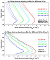 |
Fig. 1 Mean electron density profiles for different SZA range in the terminator region. Panels a shows the averaged electron density profiles, with the solid, dashed, and dotted lines representing profiles of the |IMF| = 1 nT case, |IMF| = 3 nT case, and |IMF| = 5 nT case, respectively. Panel b shows the averaged electron density profiles for the |IMF| = 3 nT case. Here, the solid and dashed lines represent profiles of the northern and southern hemispheres. The profiles are shifted on the x-axis by the amounts marked in the figure. |
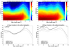 |
Fig. 2 Ionospheric upper boundary for different SZA range. Panels a and b show the mean electron density of the Martian ionosphere for an SZA range of 0°–120° and an altitude range of 120–600 km. The white line in each panel marks the altitudes that the electron density ne is equal to 100 cm−3. Panel c and d show the ionospheric upper boundary, with the solid dashed and dotted line representing the boundary of Case 1,2, and 3. The results are exhibited separately in the northern (left panels) and southern (right panels) hemispheres. |
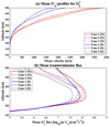 |
Fig. 3 Mean ion velocity (panel a) and mean trans-terminator ion flux (panel b) profiles along the X direction for |
![Mathematical equation: $\[\mathrm{O}_{2}^{+}\]$](/articles/aa/full_html/2025/02/aa53085-24/aa53085-24-eq9.png)
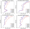 |
Fig. 4 1/e edge profile of density with respect to altitude and SZA of |
![Mathematical equation: $\[\mathrm{O}_{2}^{+}\]$](/articles/aa/full_html/2025/02/aa53085-24/aa53085-24-eq19.png)
![Mathematical equation: $\[\mathrm{CO}_{2}^{+}\]$](/articles/aa/full_html/2025/02/aa53085-24/aa53085-24-eq20.png)
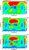 |
Fig. 5 Contour plots of horizontal velocity for |
![Mathematical equation: $\[\mathrm{O}_{2}^{+}\]$](/articles/aa/full_html/2025/02/aa53085-24/aa53085-24-eq23.png)
4 Discussion and conclusion
In this study, the impact of interplanetary magnetic field intensity on the Martian dayside and near-nightside ionosphere as well as ion transport and ion escape have been investigated. By using a 3D multifluid MHD simulation model, we revealed that the enhancement of the IMF can reduce the intrusion of solar wind into the Martian ionosphere, resulting in a smaller planetary ion outflow. The presence of a remnant magnetic field complicates the interaction between the solar wind and the ionosphere, causing an apparent north-south asymmetry in ion distribution and ion transport. Comparing our model results with previous observational studies (e.g., Dubinin et al. 2019, 2020; Fan et al. 2020; Qin et al. 2022), it can be seen that our model simulates the ionospheric flow pattern and ion density distribution successfully.
The increase in the IMF can enhance the solar wind electric field, which in turn creates a stronger induced magnetosphere. Thus, both the electric field and the magnetic field are enhanced. The enhanced electromagnetic field then protects the Martian ionosphere from the intrusion of solar wind particles. With fewer solar wind protons entering Martian space, the interactions between solar wind plasma and Martian neutral particles are weakened. Thus, the number of planetary ions generated through chemical reactions is reduced, resulting in a smaller heavy ion density and a lower ionospheric upper boundary. The energy transfer between solar wind plasma and planetary ions may also be reduced in this way, causing a lower heavy ion velocity. The vertical ion outflow flux is reduced for weak IMF conditions. Through the ion transport process, the nightside ionosphere is also influenced prominently by the variation of IMF strength. With a stronger IMF, the trans-terminator ion speed and the ion flux both decrease, causing a weaker day-to-night plasma transport to be exhibited. Therefore, the ion density of the near-nightside ionosphere is lower for high IMF strength, forming a more depleted nightside ionosphere. Both the decrease in heavy ion outflow and the weakened day-to-night plasma transport can influence the ion escape rate and lead to a lower ion escape rate, as presented in Zhang et al. (2023). However, the decrease in plasma transport dominates in this process since the ion escape in the magnetotail region is the main ion escape channel on Mars.
In our previous studies, we have shown that the enhanced solar wind dynamic pressure can increase the electromagnetic forces experienced by the planetary ions. In this way, both the outflow heavy ion flux and the day-to-night plasma transport are enhanced, facilitating the planetary ion escape. However, an increase in IMF intensity can result in a decrease in plasma transport and heavy ion outflow. Thus, in solar wind events such as interplanetary coronal mass ejection and co-rotating interaction region events, the increase in IMF intensity may partly offset the effect of the enhanced solar wind dynamic pressure on Martian heavy ions.
In addition to the IMF condition, our simulation results also present a distinct north-south asymmetry in both the ionospheric structure and the plasma transport processes. The ionosphere in the southern hemisphere is uplifted by the strong crustal field located on the dayside. The solar wind proton flux is much weaker in the southern hemisphere, which can be attributed to the shielding effect of the remnant magnetic field. Therefore, the planetary ion density is apparently higher in the southern dayside ionosphere as compared to that in the northern hemisphere, resulting in the expansion of the southern ionospheric upper boundary. The trans-terminator flow as well as the horizontal ion transport are also hindered by the crustal field. As a result, the nightside ionosphere in the northern hemisphere also tends to be more extended into the nightside. In addition, the outflow ion flux in the strong crustal field regions enhances significantly with increasing IMF intensity, contrary to the deceasing trend of the outflow flux on the global scale. Thus, it is reasonable to deduce that the enhanced IMF alters the magnetic topology near the strong crustal fields and facilitates ion outflow in these regions.
It should be noted that the MHD model used in our study adopts a 1D neutral density profile. Mechanisms such as dust storms and neutral winds are not included in this model. Thus, the Martian ionosphere simulated by our model is not influenced by the asymmetric distribution of neutral species, which leaves the crustal field to be the main endogenous source of north-south asymmetry.
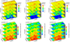 |
Fig. 6 Distribution of |
![Mathematical equation: $\[\mathrm{O}_{2}^{+}\]$](/articles/aa/full_html/2025/02/aa53085-24/aa53085-24-eq24.png)
![Mathematical equation: $\[\mathrm{O}_{2}^{+}\]$](/articles/aa/full_html/2025/02/aa53085-24/aa53085-24-eq25.png)
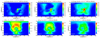 |
Fig. 7 Electromagnetic energy density ε (panels a–c) and the solar wind proton number flux nH+ · UH+ for all three cases. Both are depicted at a 1000 km altitude above the Martian surface. |
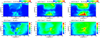 |
Fig. 8 Color plots of magnetic field strength with respect to longitude and latitude at an altitude of 900 (panels a,d), 1200 (panels b,e), and 1500 km (panels c,f) for Case 1 and Case 3. |
Acknowledgements
This work was supported by the National Natural Science Foundation of China under Grants 42241114, 42074214, and 12150008, the B-type Strategic Priority Program of the Chinese Academy of Sciences (Grant XDB41000000), and the Postdoctoral Fellowship Program of CPSF under Grant GZC20233367.
References
- Acuna, M., Connerney, J., Ness, et al. 1999, Science, 284, 790 [NASA ADS] [CrossRef] [Google Scholar]
- Acuña, M., Connerney, J., Wasilewski, P. a., et al. 1998, Science, 279, 1676 [NASA ADS] [CrossRef] [Google Scholar]
- Andrews, D. J., Stergiopoulou, K., Andersson, L., et al. 2023, JGRA, 128, e2022JA031027 [NASA ADS] [Google Scholar]
- Bougher, S., Engel, S., Roble, R., & Foster, B. 2000, JGRE, 105, 17669 [NASA ADS] [CrossRef] [Google Scholar]
- Breus, T., Ness, N., Krymskii, A., et al. 2005, AdSpR, 36, 2043 [Google Scholar]
- Cao, Y.-T., Cui, J., Wu, X.-S., Guo, J.-P., & Wei, Y. 2019, JGRE, 124, 1495 [NASA ADS] [Google Scholar]
- Chang, Q., Xu, X., Xu, Q., et al. 2020, ApJ, 900, 63 [Google Scholar]
- Chaufray, J.-Y., Gonzalez-Galindo, F., Forget, F., et al. 2014, JGRE, 119, 1614 [NASA ADS] [Google Scholar]
- Chen, R., Cravens, T., & Nagy, A. 1978, JGRA, 83, 3871 [NASA ADS] [CrossRef] [Google Scholar]
- Chu, F., Girazian, Z., Gurnett, D., et al. 2019, GRL, 46, 10257 [NASA ADS] [CrossRef] [Google Scholar]
- Cui, J., Galand, M., Yelle, R., Wei, Y., & Zhang, S.-J. 2015, JGRA, 120, 2333 [NASA ADS] [Google Scholar]
- Cui, J., Rong, Z., Wei, Y., & Wang, Y. 2020, E&PP, 4, 1 [CrossRef] [Google Scholar]
- Diéval, C., Morgan, D., Němec, F., & Gurnett, D. 2014, JGRA, 119, 4077 [Google Scholar]
- Dong, C., Bougher, S. W., Ma, Y., et al. 2014, GRL, 41, 2708 [NASA ADS] [CrossRef] [Google Scholar]
- Dong, C., Ma, Y., Bougher, S. W., et al. 2015, GRL, 42, 9103 [NASA ADS] [CrossRef] [Google Scholar]
- Dong, C., Bougher, S. W., Ma, Y., et al. 2018, JGRA, 123, 6639 [NASA ADS] [Google Scholar]
- Dong, Y., Fang, X., Brain, D., et al. 2019, JGRA, 124, 4295 [NASA ADS] [Google Scholar]
- Dubinin, E., Fränz, M., Pätzold, M., et al. 2018, P&SS, 160, 56 [NASA ADS] [CrossRef] [Google Scholar]
- Dubinin, E., Fränz, M., Pätzold, M., et al. 2019, JGRA, 124, 9725 [NASA ADS] [Google Scholar]
- Dubinin, E., Fränz, M., Pätzold, M., et al. 2020, JGRA, 125, e2020JA028010 [Google Scholar]
- Duru, F., Gurnett, D., Frahm, R., et al. 2009, JGRA, 114, A12 [CrossRef] [Google Scholar]
- Duru, F., Baker, N., De Boer, M., et al. 2020, JGRA, 125, e2019JA027409 [Google Scholar]
- Edberg, N., Lester, M., Cowley, S., & Eriksson, A. 2008, JGRA, 113, A08206 [NASA ADS] [CrossRef] [Google Scholar]
- Edberg, N., Brain, D., Lester, M., et al. 2009, AnGeo, 27, 3537 [Google Scholar]
- Fan, K., Fraenz, M., Wei, Y., et al. 2019, GRL, 46, 11764 [NASA ADS] [CrossRef] [Google Scholar]
- Fan, K., Fraenz, M., Wei, Y., et al. 2020, ApJ, 898, L54 [Google Scholar]
- Fan, K., Wei, Y., Fraenz, M., et al. 2023, GRL, 50, e2023GL103999 [NASA ADS] [CrossRef] [Google Scholar]
- Fang, X., Ma, Y., Masunaga, K., et al. 2017, JGRA, 122, 4117 [NASA ADS] [Google Scholar]
- Fang, X., Ma, Y., Luhmann, J., et al. 2023, JGRA, 128, e2023JA031588 [NASA ADS] [Google Scholar]
- Flynn, C. L., Vogt, M. F., Withers, P., et al. 2017, GRL, 44, 10 [NASA ADS] [CrossRef] [Google Scholar]
- Fowler, C., Andersson, L., Ergun, R., et al. 2015, GRL, 42, 8854 [NASA ADS] [CrossRef] [Google Scholar]
- Fowler, C. M., Hanley, K. G., McFadden, J., et al. 2022, JGRA, 127, e2022JA030726 [NASA ADS] [Google Scholar]
- Gao, J., Rong, Z., Klinger, L., et al. 2021, E&SS, 8, e2021EA001860 [Google Scholar]
- Garnier, P., Jacquey, C., Gendre, X., et al. 2022, JGRA, 127, e2021JA030147 [Google Scholar]
- Girazian, Z., Mahaffy, P., Lillis, R., et al. 2017a, GRL, 44, 11 [NASA ADS] [CrossRef] [Google Scholar]
- Girazian, Z., Mahaffy, P., Lillis, R., et al. 2017b, JGRA, 122, 4712 [NASA ADS] [Google Scholar]
- Gurnett, D., Huff, R., Morgan, D., et al. 2008, AdSpR, 41, 1335 [Google Scholar]
- Halekas, J., Brain, D., Luhmann, J., et al. 2017, JGRA, 122, 11 [NASA ADS] [Google Scholar]
- Harnett, E., & Winglee, R. 2003, GRL, 30, 20 [NASA ADS] [CrossRef] [Google Scholar]
- Jakosky, B. M., & Phillips, R. J. 2001, Nature, 412, 237 [NASA ADS] [CrossRef] [Google Scholar]
- Jakosky, B. M., Slipski, M., Benna, M., et al. 2017, Science, 355, 1408 [CrossRef] [Google Scholar]
- Kallio, E., Barabash, S., Janhunen, P., & Jarvinen, R. 2008, P&SS, 56, 823 [NASA ADS] [CrossRef] [Google Scholar]
- Lammer, H., Chassefière, E., Karatekin, O., et al. 2013, SSRv, 174, 113 [NASA ADS] [Google Scholar]
- Ledvina, S. A., Brecht, S. H., Brain, D. A., & Jakosky, B. M. 2017, JGRA, 122, 8391 [NASA ADS] [Google Scholar]
- Li, S., Lu, H., Cui, J., et al. 2020, E&PP, 4, 23 [NASA ADS] [Google Scholar]
- Li, S., Lu, H., Cao, J., et al. 2022a, ApJ, 941, 198 [NASA ADS] [CrossRef] [Google Scholar]
- Li, S., Lu, H., Cao, J., et al. 2022b, ApJ, 931, 30 [Google Scholar]
- Lillis, R. J., Fillingim, M. O., Peticolas, L. M., et al. 2009, JGRE, 114, E11009 [CrossRef] [Google Scholar]
- Liu, D., Rong, Z., Gao, J., et al. 2021, ApJ, 911, 113 [NASA ADS] [CrossRef] [Google Scholar]
- Ma, Y., Nagy, A. F., Sokolov, I. V., & Hansen, K. C. 2004, JGRA, 109, A07211 [NASA ADS] [Google Scholar]
- Ma, Y., Fang, X., Nagy, A., Russell, C., & Toth, G. 2014, JGRA, 119, 1272 [NASA ADS] [Google Scholar]
- Ma, Y., Russell, C., Fang, X., et al. 2017, JGRA, 122, 1714 [NASA ADS] [Google Scholar]
- Matsunaga, K., Seki, K., Brain, D. A., et al. 2017, JGRA, 122, 9723 [NASA ADS] [Google Scholar]
- McKay, C. P., & Stoker, C. R. 1989, RvGeo, 27, 189 [NASA ADS] [Google Scholar]
- Morgan, D., Gurnett, D., Kirchner, D., et al. 2008, JGRA, 113, A09303 [NASA ADS] [CrossRef] [Google Scholar]
- Najib, D., Nagy, A. F., Tóth, G., & Ma, Y. 2011, JGRA, 116, A05204 [NASA ADS] [CrossRef] [Google Scholar]
- Němec, F., Morgan, D., Gurnett, D., & Duru, F. 2010, JGRE, 115, A11314 [Google Scholar]
- Qin, J., Zou, H., Ye, Y., Hao, Y., & Wang, J. 2022, Icarus, 388, 115255 [NASA ADS] [CrossRef] [Google Scholar]
- Ramstad, R., Brain, D. A., Dong, Y., et al. 2020, Nat. Astron., 4, 979 [CrossRef] [Google Scholar]
- Sakai, S., Seki, K., Terada, N., et al. 2021, JGRA, 126, e2020JA028485 [Google Scholar]
- Sakai, S., Seki, K., Terada, N., et al. 2023, JGRA, 128, e2022JA030510 [NASA ADS] [Google Scholar]
- Sánchez-Cano, B., Narvaez, C., Lester, M., et al. 2020, JGRA, 125, e2020JA028145 [Google Scholar]
- Shizgal, B. D., & Arkos, G. G. 1996, RvGeo, 34, 483 [NASA ADS] [Google Scholar]
- Song, Y., Lu, H., Cao, J., et al. 2023a, JGRA, 128, e2022JA031083 [NASA ADS] [Google Scholar]
- Song, Y., Lu, H., Cao, J., et al. 2023b, JGRA, 128, e2023JA031788 [NASA ADS] [Google Scholar]
- Vogt, M. F., Withers, P., Mahaffy, P. R., et al. 2015, GRL, 42, 8885 [NASA ADS] [CrossRef] [Google Scholar]
- Wang, M., Lee, L., Xie, L., et al. 2021, A&A, 651, A22 [NASA ADS] [CrossRef] [EDP Sciences] [Google Scholar]
- Weber, T., Brain, D., Xu, S., et al. 2020, GRL, 47, e2020GL087757 [NASA ADS] [CrossRef] [Google Scholar]
- Withers, P. 2009, AdSpR, 44, 277 [Google Scholar]
- Withers, P., Fillingim, M., Lillis, R., et al. 2012, JGRA, 117, A12307 [NASA ADS] [CrossRef] [Google Scholar]
- Wordsworth, R. D. 2016, AREPS, 44, 381 [NASA ADS] [Google Scholar]
- Xu, S., Fang, X., Mitchell, D. L., et al. 2018, GRL, 45, 7337 [NASA ADS] [CrossRef] [Google Scholar]
- Xu, S., Curry, S. M., Mitchell, D. L., et al. 2019, JGRA, 124, 151 [NASA ADS] [Google Scholar]
- Xu, S., Mitchell, D. L., Weber, T., et al. 2020, JGRA, 125, e2020JA028576 [Google Scholar]
- Zhang, M., Luhmann, J., & Kliore, A. 1990, JGRA, 95, 17095 [NASA ADS] [CrossRef] [Google Scholar]
- Zhang, Q., Holmström, M., Wang, X.-d., Nilsson, H., & Barabash, S. 2023, JGRA, 128, e2023JA031828 [NASA ADS] [Google Scholar]
- Zhang, Q., Barabash, S., Holmstrom, M., et al. 2024, Nature, 1, 45 [NASA ADS] [CrossRef] [Google Scholar]
All Tables
All Figures
|
Fig. 1 Mean electron density profiles for different SZA range in the terminator region. Panels a shows the averaged electron density profiles, with the solid, dashed, and dotted lines representing profiles of the |IMF| = 1 nT case, |IMF| = 3 nT case, and |IMF| = 5 nT case, respectively. Panel b shows the averaged electron density profiles for the |IMF| = 3 nT case. Here, the solid and dashed lines represent profiles of the northern and southern hemispheres. The profiles are shifted on the x-axis by the amounts marked in the figure. |
| In the text | |
|
Fig. 2 Ionospheric upper boundary for different SZA range. Panels a and b show the mean electron density of the Martian ionosphere for an SZA range of 0°–120° and an altitude range of 120–600 km. The white line in each panel marks the altitudes that the electron density ne is equal to 100 cm−3. Panel c and d show the ionospheric upper boundary, with the solid dashed and dotted line representing the boundary of Case 1,2, and 3. The results are exhibited separately in the northern (left panels) and southern (right panels) hemispheres. |
| In the text | |
|
Fig. 3 Mean ion velocity (panel a) and mean trans-terminator ion flux (panel b) profiles along the X direction for |
| In the text | |
|
Fig. 4 1/e edge profile of density with respect to altitude and SZA of |
| In the text | |
|
Fig. 5 Contour plots of horizontal velocity for |
| In the text | |
|
Fig. 6 Distribution of |
| In the text | |
|
Fig. 7 Electromagnetic energy density ε (panels a–c) and the solar wind proton number flux nH+ · UH+ for all three cases. Both are depicted at a 1000 km altitude above the Martian surface. |
| In the text | |
|
Fig. 8 Color plots of magnetic field strength with respect to longitude and latitude at an altitude of 900 (panels a,d), 1200 (panels b,e), and 1500 km (panels c,f) for Case 1 and Case 3. |
| In the text | |
Current usage metrics show cumulative count of Article Views (full-text article views including HTML views, PDF and ePub downloads, according to the available data) and Abstracts Views on Vision4Press platform.
Data correspond to usage on the plateform after 2015. The current usage metrics is available 48-96 hours after online publication and is updated daily on week days.
Initial download of the metrics may take a while.