| Issue |
A&A
Volume 694, February 2025
|
|
|---|---|---|
| Article Number | A50 | |
| Number of page(s) | 12 | |
| Section | Planets, planetary systems, and small bodies | |
| DOI | https://doi.org/10.1051/0004-6361/202450449 | |
| Published online | 31 January 2025 | |
Instantaneous asymmetry of the Martian bow shock: A single- and dual-spacecraft study using MAVEN and Mars Express
1
Department of Physics, Umeå University,
901 87
Umeå,
Sweden
2
Department of Mathematics, Physics and Electrical Engineering, Northumbria University,
Newcastle upon Tyne,
UK
★ Corresponding author; This email address is being protected from spambots. You need JavaScript enabled to view it.
Received:
19
April
2024
Accepted:
22
November
2024
Abstract
Aims. We study the instantaneous asymmetry of the Martian bow shock during a change in the direction of the interplanetary magnetic field (IMF) and for steady-state conditions. Specifically, we study the asymmetry with regard to the convective electric field and to the crustal fields of Mars.
Methods. Two methods were used: First, a single-spacecraft method in which a switch in hemisphere in the Mars solar-electric (MSE) coordinate system was studied during a change in the direction of the interplanetary magnetic field. Second, we used a dual-spacecraft method wherein near simultaneous bow shock crossings on opposite hemispheres were studied. The dual bow shock crossings were then compared to a bow shock model, and the difference in the distance to the model was used as a measure of asymmetry.
Results. With the single-spacecraft method, an asymmetry with respect to the solar wind convective electric field, Esw, was found, wherein the bow shock was farther from the planet in the ZMSE <0 hemisphere, that is, the −E hemisphere. With the dual-spacecraft method, the mean of the magnitude of the asymmetries in the individual case was 0.13 RM. However, the standard deviation was as high as the mean, and no significant asymmetry could be attributed either to the solar wind convective electric field or to the Martian crustal fields. A strong asymmetry without a clear correlation to these factors was found nonetheless. Possible causes of the measured asymmetry are discussed.
Conclusions. The magnitude of the asymmetries in individual observations is larger than the average asymmetries. This indicates that the shape of the Martian bow shock is dynamic and influenced by fluctuations or wave phenomena.
Key words: plasmas / shock waves / planets and satellites: dynamical evolution and stability / planets and satellites: general / planets and satellites: magnetic fields
© The Authors 2025
 Open Access article, published by EDP Sciences, under the terms of the Creative Commons Attribution License (https://creativecommons.org/licenses/by/4.0), which permits unrestricted use, distribution, and reproduction in any medium, provided the original work is properly cited.
This article is published in open access under the Subscribe to Open model. This email address is being protected from spambots. You need JavaScript enabled to view it. to support open access publication.
1 Introduction
The bow shock is the first interaction region between the solar wind and the magnetosphere of the Martian system (Slavin & Holzer 1982; Schwingenschuh et al. 1990; Möhlmann et al. 1992, e.g.). It is created when the supersonic solar wind meets the ionosphere of Mars. The flow becomes shocked and is decelerated and deflected around the ionosphere (Yi et al. 1999; Mazelle et al. 2004). The interplanetary magnetic field (IMF) of the solar wind is frozen into the plasma and will therefore pile up, and together with the shocked flow, it will create a region with a higher particle density and magnetic field strength behind the bow shock. This is known as the magnetosheath (Dubinin et al. 1997; Vaisberg et al. 2018). Over long timescales and spatial scales, the system is in a steady-state: The bow shock is a constant presence between the solar wind and the magnetosheath. On smaller timescales and spatial scales, the system is remarkably dynamic, however: The shock is continuously reformed, and the position and shape of the shock change continuously (Hall et al. 2019; Romanelli et al. 2019; Madanian et al. 2020). The Martian system is interesting in that it is a hybrid system in which the shock is formed both in the interaction with the ionosphere, which gives rise to what is called an induced magnetosphere (Luhmann et al. 2004; Bertucci et al. 2011, e.g.), and in the interaction with the Martian crustal fields, which are strong enough to stand-off the solar wind (Brain et al. 2003).
Previous research has shown that the Martian bow shock is not symmetric, and several factors contribute to the asymmetry. There is an asymmetry with respect to the direction of the IMF; regions in which the bow shock normal is quasi-parallel to the IMF are closer to the planet than regions in which it is quasiperpendicular (Zhang et al. 1991; Vignes et al. 2002; Garnier et al. 2022a). The asymmetry with respect to the solar wind convective electric field (Esw) at Mars has been debated. There is a clear asymmetry in the ion flows at Mars, with Esw accelerating particles, creating an ion plume (Fang et al. 2008; Dong et al. 2015). Vignes et al. (2002) found that the bow shock was farther from the planet in the hemisphere of locally upward Esw . This result was also found by Edberg et al. (2009). Garnier et al. (2022a) found that particle acceleration by Esw could introduce asymmetries, but that this driver is secondary to other factors. Other studies did not report a significant asymmetry in the direction of the electric field (Halekas et al. 2017; Fang et al. 2017; Gruesbeck et al. 2018), but they did not use near simultaneous observations of bow shock crossings, or in the case of Fang et al. (2017), they used a magnetohydrodynamic fluid model, which might fail to capture kinetic effects. An asymmetry with respect to the electric field has been found at other planetary bodies. At comet 67P/Churyumov-Gerasimenko, observations and simulations showed a strong asymmetry with respect to Esw (Gunell et al. 2018). Comparisons between Mars and comets are interesting because the particle gyration radius and the size of the magnetosphere have similar scale ratios, which means that kinetic effects are important.
The asymmetry due to crustal fields is likewise debated. Edberg et al. (2009) found only a weak correlation between the strong crustal field region and larger bow shock stand-off distance, whereas other studies have found stronger evidence. Edberg et al. (2008) found that bow shock crossings that occurred over the southern hemisphere were farther out than crossings over the northern hemisphere on average, which they hypothesized might be caused by the crustal fields. Gruesbeck et al. (2018) similarly found a significant north-south asymmetry that they thought to be caused by crustal fields. The simulations by Fang et al. (2017) showed that the crustal fields significantly affected the location of the bow shock. Garnier et al. (2022b) used a multi-spacecraft approach to study the effect of crustal fields on the bow shock location. They found that it was a secondary driver after extreme-ultraviolet (EUV) flux and the magnetosonic Mach number (MMS).
The bow shock location as a whole is affected by the solar wind conditions. The main drivers for the bow shock location are the solar EUV flux, MMS, and the solar wind dynamic pressure (Pdyn) (Garnier et al. 2022a). The solar EUV flux affects the bow shock by ionizing planetary atoms and molecules, which increases the pressure in the magnetosheath, thereby pushing the bow shock outward from the planet. An increased EUV flux therefore increases the bow shock altitude (Halekas et al. 2017; Garnier et al. 2022a). Edberg et al. (2010) showed that an increase in MMS decreases the bow shock altitude, and (Halekas et al. 2017) later confirmed these results. The effect of the solar wind dynamic pressure on the bow shock location is well documented: A higher solar wind dynamic pressure pushes the bow shock closer to the planet (Schwingenschuh et al. 1992; Trotignon et al. 1993; Halekas et al. 2017). The effect is secondary to that of EUV and MMS, however (Garnier et al. 2022a).
Currently, there are no multi-spacecraft missions at Mars, but many have been proposed (Sanchez-Cano et al. 2022; Lillis et al. 2021; Larkin et al. 2024), and the dual-spacecraft mission EscaPADE is set to launch within the next few years (Lillis et al. 2022). It is at present difficult to study different regions of Mars simultaneously. In our study, we aim to combine the data sets of the Mars Express (MEX) and Mars Atmosphere and Volatile Evolution (MAVEN) mission to obtain near simultaneous measurements, such that the instantaneous asymmetry of the bow shock can be studied. The lack of multi-spacecraft missions also means that it is difficult to study the dynamics of the system because few simultaneous measurements of the upstream solar wind and the response of the magnetosphere are available. Our study aims to overcome this limitation by studying a shift in the IMF direction. When transformed into a coordinate system that is aligned with the solar convective electric field, the spacecraft switches position from one hemisphere to the other during a flip in the magnetic field direction, thereby allowing us to study the response in the magnetosphere to the change in upstream conditions.
To study the temporal and spatial variations in the Martian bow shock, we used two different methods. First, we used MAVEN data to study the effect of a shift in the magnetic field on the magnetosphere. As there is no solar wind monitor, the calm conditions after an interplanetary coronal mass ejection (ICME) (Tsurutani et al. 2008) were chosen to better isolate the phenomena we wish to study. Second, we used near simultaneous measurements by MAVEN and MEX to study the potential asymmetry of the Martian bow shock. Events in which the two spacecraft cross the bow shock on opposing hemispheres were compared with a bow shock model to determine the difference in the observed crossings from a symmetrical paraboloid.
This paper is structured in the following way: In Section 2, Instrumentation, we describe the spacecraft and data sets, including the instruments with which the data were obtained. The results of the two different methods are described in Section 3, where the results of the single-spacecraft method are presented in Section 3.1, and the results of the dual-spacecraft study are described in Section 3.2. We discuss the results and present our conclusions in Section 4.
2 Instrumentation
The data we used come from the MAVEN (Jakosky et al. 2015) and MEX (Chicarro et al. 2004) missions. The data stem from 2014 to 2021 and span parts of solar cycles 24 and 25 (NOAA 2023).
The MAVEN mission went into orbit around Mars in September 2014 and hosts a suite of plasma instruments. We made use of magnetic field data from the Magnetometer (MAG) (Connerney et al. 2015), which measures the vector magnetic field with a 0.05 nT resolution and a measurement frequency of 32 s−1 . Electron data were acquired from the Solar Wind Electron Analyzer (SWEA) (Mitchell et al. 2016), an electrostatic analyzer with a field of view (FOV) of 2π, an energy range of 5 eV − 4.6 keV, and a measurement frequency of 0.5 s−1. The ion data were acquired from the Solar Wind Ion Analyzer (SWIA) (Halekas et al. 2015), which is also an electrostatic analyzer with a FOV of 2π, an energy range of 5 eV/q–25 keV/q, and a measurement frequency of 0.25 s−1. The solar EUV flux was measured by the Extreme Ultraviolet (EUV) Monitor (Eparvier et al. 2015), which measures the solar emissions in three distinct energy bands. These data then served as input to the flare irradiance spectral model (FISM), which provides a model for the whole spectrum (Thiemann et al. 2017). We used the whole spectrum to determine the solar EUV flux.
MEX arrived at Mars in 2003 and is still providing measurements of the red planet in 2024. It carries a suite of particle instruments, the Analyzer of Space Plasmas and Energetic Atoms (ASPERA-3) (Barabash et al. 2006), which was used in this study. The Electron Spectrometer (ELS) is most important for our study (Barabash et al. 2006). This is a top-hat electrostatic analyzer with an energy range of 0.01–20 keV and a measurement frequency of 0.25 s−1. This energy spectrum is divided into two data products, with a lower and higher energy range. Most of the spectrum here was covered by the lower energy range, and therefore, only the lower energy range was used. The ion measurements were provided by the Ion Mass Analyzer (IMA) (Barabash et al. 2006), which is an electrostatic analyzer with an energy range of 0.01–36 keV/q for ions H+, He2+, He+, and O+ . It makes a full sweep of its FOV in 3 minutes and 12 seconds.
We used several coordinate systems in order to best represent different asymmetries. In the Mars-centered solar orbital (MSO) coordinate system, the x-axis points from Mars to the Sun, the y-axis points antiparallel to the orbital velocity of Mars, and the z-axis completes the right-handed system. In the Mars solarelectrical (MSE) coordinate system, the x-axis points antiparallel to the solar wind bulk velocity, the z-axis is parallel to Esw of the solar wind, and the y-axis completes the right-handed system. The MSE coordinate system is useful for discerning an asymmetry with respect to the electric field because unless there is a sampling bias, it evens out asymmetries with respect to the crustal fields, the magnetic field alignment, and so on. The system is typically divided into two hemispheres. The + E and − E hemisphere is defined by ZMS E >0 and ZMS E <0, respectively.
To investigate the effect of the crustal fields on the Martian bow shock location, the bow shock crossing position was projected onto the longitude and latitude on Mars to investigate whether a crossing occurred over a region with a high or low crustal field strength. MEX and MAVEN both use a planetographic coordinate system for the data used in this study. In the planetographic coordinate system, the origin is the center of mass, and the north pole (+90°) is defined as the rotational pole on the north side of the invariable plane of the Solar System (Withers & Jakosky 2017). The equator represents 0° latitude, and the south pole is at −90°. The other latitudes are defined relative to a reference ellipsoid with a polar radius 3376.20 km and an equatorial radius of 3396.19 km.
3 Method and observations
3.1 Single-spacecraft method: MAVEN
In this section, we use a single spacecraft (MAVEN) to assess the asymmetries in the Martian bow shock depending on the convective electric field of the solar wind. This is done by examining the plasma properties immediately before and after a change in the IMF direction, which rotates the MSE coordinate system, while the spacecraft does not move significantly in the MSO system. In order to minimize the influence of other changes, we considered periods following the passage of an ICME, when the solar wind is expected to be calmer than usual (Tsurutani et al. 2008). This method was previously employed in observations of the infant bow shock (IBS) of comet 67P/Churyumov-Gerasimenko (67P) (Gunell et al. 2018; Goetz et al. 2021).
3.1.1 Method
We examined the intervals that were identified as ICMEs at Mars by Zhao et al. (2021). The ion spectrograms recorded by the SWIA instrument during these intervals were examined for signatures similar to those of the IBS observations at comet 67P. Then the set of events was narrowed down further by including only events with a clear change between the + E and −E hemispheres.
In order to determine in which hemisphere with respect to the solar wind convective electric field the spacecraft is before, during, and after the directional change in the IMF, we defined cos θ following Gunell et al. (2018). This quantity is the cosine of the angle between the projections onto the yMSO−zMSO plane of the convective electric field of the solar wind, Esw = −vsw × Bsw, and the Mars-to-spacecraft vector,
 (1)
(1)
where ux, uy, and uz are unit vectors in the xMSO, yMSO, and zMSO directions, respectively, and B is the magnetic field at the spacecraft position, which is used as an approximation of the IMF. Assuming vsw = −|vsw|ux, we obtain
 (2)
(2)
Thus, cos θ is a normalized measure of
 (3)
(3)
The electron energy flux is greater in the magnetosheath than in the solar wind. We integrated the differential energy flux of the electrons, Γe measured by the SWEA instrument, to obtain a quantity, Fe, that can be used to determine in which hemisphere the spacecraft is located in the magnetosheath as opposed to the solar wind. We define
 (4)
(4)
where the upper limit of the integral, 4600 eV, is the upper limit of the SWEA energy range, and the lower limit, 30 eV, was chosen to exclude contributions from photoelectrons. Fe was normalized to 1010 eV/(cm2 s sr) as it is only used as a relative measure. A low Fe value corresponds to the solar wind, and a high Fe value corresponds to the magnetosheath.
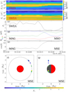 |
Fig. 1 Single-spacecraft observation. Example from 7 October 2015, showing a case when magnetosheath plasma was found in the −E hemisphere. (a) Logarithm of the differential energy flux of the ions in units of eV/(cm2s sr eV), (b) logarithm of the differential energy flux of the electrons in units of eV /(cm2s sr eV), (c) normalized integrated electron energy flux Fe, (d) magnetic flux density components, (e) normalized zMSE coordinate cos θ, (f) Fe (color-coded) at the positions of the observation in the yMSE − zMSE plane, and (g) Fe (color-coded) at the positions of the observation in the xMSE− zMSE plane. The magnetosheath is characterized by a higher electron flux Fe, as shown in panels c, f, and g. The −E hemisphere corresponds to cos θ < 0. |
3.1.2 Results
Using the event-selection procedure described in Sect. 3.1.1, we found ten events that could be used to detect asymmetries between the −E and + E hemispheres. An example from 7 October 2015 is shown in Fig. 1. In panels a and b, the differential energy flux of ions and electrons is shown, and panel d shows the components of the magnetic flux density. The derived quantities FE and cos θ are shown in panels c and e, respectively. For this event, as for all the others, we plotted 75 s of data. At the beginning of the interval, the spacecraft was located in the magnetosheath, where the protons are slower and warmer than in the solar wind (Fig. 1a), and the electron flux is higher (Figs. 1b and c). The spacecraft was located in the −E hemisphere at the start of the interval (cos θ < 0, panel e), and around 01:16:20, the magnetic field changed direction (Fig. 1d) and the spacecraft entered the + E hemisphere, where cos θ > 0 (Fig. 1e). The spacecraft was at x ≈ −0.6 RM at the time of observation, as shown in the map in Fig. 1g. Thus, the bow shock was closer to the x axis in + E than in −E for x ≈ −0.6 RM. In the hybrid simulations by Kallio et al. (2006), the observation held for x ≈ −0.6 RM (their Fig. 4b). However, the structure of the plasma in their simulation also indicated significant fluctuations in the +E hemisphere, and a single observation might deviate non-negligibly from the average.
Fluctuations during the transition between the hemispheres are seen in the example from 10 March 2018, which is shown in Fig. 2. In this event, Fe gradually decreased starting at approximately 15:51:30 and reached a stable low value at 15:51:50, showing that the spacecraft moved from the magnetosheath into the solar wind. Fig. 2e shows that cos θ fell from +1 down to −1 during the same period. This means that magnetosheath plasma was observed in the +E hemisphere, that is to say, opposite of where it was in Fig. 1. The observation took place near the terminator and covered the positive and negative zMSE axis.
All events are summarized in Table 1, where we indicate in which hemisphere magnetosheath plasma was found. In two of the events the spacecraft transitioned twice between the MSE hemispheres. The number of hemisphere transitions is indicated by the quantity NHC in Table 1. The fluctuations mentioned above affect the value of cos θ during the transition, as Fig. 2 shows. While most events are calm, fluctuations were also detected in the event that occurred at 19:10:40 on 9 March 2015. Table 1 also includes values of the angle θBn between the IMF and the shock normal, the dynamic pressure pdyn, and the Alfvénic Mach number MA . These values refer to the situation when MAVEN was on the solar wind side of the shock, which is necessary as solar wind values are inaccessible when the spacecraft is in the magnetosheath. There is no systematic relation between θBn, pdyn, and MA and whether magnetosheath plasma was detected in the +E or −E hemisphere. Table 1 also lists the EUV intensity of the entire spectrum of the EUV monitor (see Sect. 2). The values for the two cases when the magnetosheath was observed in the +E hemisphere are within the range of those for magnetosheath observations in the −E hemisphere. Thus, there is no indication that the results were influenced by the EUV flux. Similarly, information about whether the spacecraft crossed the bow shock over a region of strong crustal fields was added in the penultimate column. For most of the events, the spacecraft is not over the crustal field region (as expected because most of Mars is not covered by strong crustal fields). The two events that took place over the crustal field region occurred when magnetosheath plasma was found in the −E hemisphere, but so were seven other events. In conclusion, crustal fields were unlikely to affect the results. The last column of Table 1 shows the planetocentric distance rsc of the observations and is included for reference. Since the spacecraft did not move appreciably while the magnetic field changed direction, the spacecraft was on either side of the bow shock and in both hemispheres for the same rsc value, and it is therefore not expected to influence the result. The influence of different drivers of the bow shock position is discussed further in Sect. 4.
Magnetosheath plasma was found in the −E hemisphere in eight and in the +E hemisphere in two of the ten cases. The null hypothesis that there is no asymmetry and that the spacecraft can appear in either hemisphere with an equal probability of 50%, has a 5.5% risk of yielding this result. As the spacecraft does not move significantly during the 75 s interval, the best that can be done with this method is to determine whether an asymmetry exists. We cannot obtain a measurement of how strong this asymmetry is. We can say with a 94% degree of confidence that the bow shock is asymmetric, with the bow shock being farther from the x-axis in the −E hemisphere than in the +E hemisphere.
List of single-spacecraft MAVEN events.
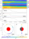 |
Fig. 2 Single-spacecraft observation. Example from 10 March 2018, showing a case when magnetosheath plasma was found in the +E hemisphere. (a) Logarithm of the differential energy flux of the ions in units of eV/(cm2s sr eV), (b) logarithm of the differential energy flux of the electrons in units of eV /(cm2s sr eV), (c) normalized integrated electron energy flux Fe, (d) magnetic flux density components, (e) normalized zMSE coordinate cos θ, (f) Fe (color-coded) at the positions of observation in the yMSE–zMSE plane, and (g) Fe (color-coded) at the positions of observation in the xMSE–zMSE plane. The magnetosheath is characterized by a higher electron flux Fe, as shown in panels c, f, and g. The −E hemisphere corresponds to cos θ < 0. |
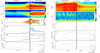 |
Fig. 3 Data from an example event where MAVEN and MEX crossed the bow shock within 10 minutes of each other. The left side shows MAVEN data, and the panels show (a) the electron energy spectrogram, (b) the ion energy spectrogram, (c) the magnetic field, (d) the ion density, (e) the ion bulk velocity, and (f) the spacecraft position. The right plot shows MEX data, and the panels show (g) the electron energy spectrogram, (h) the ion energy spectrogram, (i) the proton density, (j) the proton velocity, and (k) the spacecraft position. The arrows above the two figures indicate the regions through which the spacecraft traveled. The vertical black line shows the manually chosen bow shock crossing. All data are given in the MSO coordinate system. |
3.2 Dual-spacecraft analysis: MAVEN and MEX
3.2.1 Method
The events chosen for the dual-spacecraft method followed certain criteria. The spacecraft had to be within 1.5 RM < xMSO < 1.8 RM in the x-direction in MSO coordinates. The two spacecraft had to be within 45 degrees of the subsolar point, and the spacecraft had to be separated by at least 45 degrees. Since MEX only sends back telemetry from the instruments for certain periods, only times for which MEX electron and ion data were available were chosen. When we applied these criteria, we found 20 events in total. In 11 of these 20 events, the spacecraft crossed in different E hemispheres, and in 11 events one spacecraft was above a region with a large crustal field strength, and in one event, it was above a region with a small crustal field strength.
The bow shock crossings were identified as a broadening in the electron spectrogram. These data was chosen because they had the highest time resolution for MEX (since it lacks a magnetometer), and it was deemed best to identify the crossing in the electron data also for MAVEN. An example of an event is shown in Figure 3. In Figures 3a and 3b, we show the bow shock crossings measured by MAVEN and MEX, respectively. In Figure 3a, at 13:49:55 we show the broadening of the electron spectrogram, which indicates the heating of the electrons and signifies the bow shock crossing. A similar broadening can be seen slightly later in the ion spectrogram in panel b. Simultaneous with the broadening of the electron spectrogram, an increase in the magnetic field is shown in panel c. This corresponds to the pile-up of the magnetic field at the bow shock (Trotignon et al. 2006). In panels d and e, we show an increase in the ion density and a decrease in the ion bulk velocity, and in the last panel f, the spacecraft position is shown. The arrows at the top of the figure indicate the solar wind and magnetosheath regions. The averages for the solar wind conditions were taken in the region shown as solar wind.
The accompanying bow shock crossing measured by MEX is shown in Fig. 3b. In panel g, we show the electron energy spectrogram, in which the broadening of the spectrogram signifies the bow shock crossing at 13:46:49. The following panels show (h) the ion spectrogram (wherein the periodic maxima is an effect of the 192-second instrument sweep), (i) the proton density, (j) the proton velocity, and (k) the spacecraft position. The different regions are similar as in 3a shown at the top.
To measure the asymmetry of the bow shock, the measured bow shock crossings were compared to a bow shock model. Since the bow shock is not shaped like half a sphere, but like a paraboloid, the distance to the planet surface would be misleading. Therefore, we instead measured the distance from the actual measured crossing to the bow shock model. The bow shock model was developed by Ramstad et al. (2017) and takes the solar wind density and bulk velocity as input, which we acquired from MAVEN data upstream of the bow shock at 1 min average. The model is limited in which drivers it takes as input, which limits its accuracy. However, the exact placement of the bow shock model is not a necessity in this study because we are interested in the difference between the distances to the bow shock. Therefore, the limitations of the model are not a hindrance to the study. The measure of asymmetry was defined as follows: The distance from the observed crossing to the bow shock model was d1 and d2 for each spacecraft, respectively, and we defined Δd as the difference between these distances, Δd = d1 − d2 (see Figure 4). When a crossing was measured inside the bow shock, this distance d would be negative. Δd therefore is a measure of the divergence from symmetry because if the bow shock were perfectly symmetrical around the x-axis, Δd would be zero. In order to quantify Δd compared to a typical distance from the origin to the bow shock, a scale length for the dataset was calculated. It was defined as the mean of the distances from the observed crossings to the origin of the MSO coordinate system,
 (5)
(5)
Here, ri is the distance from the observed bow shock crossing to the origin of the MSO system, and N is the total number of bow shock crossings (which is 40, as there are in total 20 events, and each event is a pair of bow shock crossings). This value was calculated in order to estimate a percent value on |Δd|, that is, the asymmetry. This value is an average, however, because the distance to the bow shock from the origin is dependent on location on the bow shock, as for example the distance increases toward the flanks. The calculated scale length was 1.667 RM.
3.2.2 Comparison of MAVEN and MEX
This ection describes the results pertaining to all 20 events for which the asymmetry was studied without considering a particular cause. The average time difference between the crossings was 12.4 minutes, the largest time difference was 40.8 minutes, and the smallest time difference was 1.2 minutes. The locations of the crossings are shown in Figure 5. The crossings are spread out over the dayside, with slight concentrations at about 45° from the Mars-Sun line. No systematic difference between the northern and southern hemisphere can be seen. A histogram of Δd for all of the events is shown in Figure 6. Because we studied the divergence from symmetry by any cause, we did not wish positive and negative Δd to cancel out when we calculated the mean. Therefore, the absolute value of the difference in the distance to the bow shock model was used, |Δ d| = |dmav − dmex |. The figure shows that |Δd| was most commonly in the range 0–0.175 RM, with 4 out of 20 events showing larger |Δd| than this range. The average difference in the distance from the observed crossing to the bow shock model, |Δd|, was 0.13±0.13 RM. Using the scale length, Ls, as given by Equation (5), we calculated the average percent asymmetry, which for this data set was 0.13/1.667 = 7.8%, with one standard deviation of 0.13/1.667 = 7.8% (the mean and the standard deviation were the same up to two significant digits). The error, as denoted by the error bar in the upper right corner, stems from the time resolution of the position of MEX. The largest change in position between two time steps was 45 km, which means that this is the largest error due to the time resolution. There is no significant difference between the estimates by the two spacecraft.
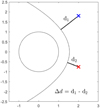 |
Fig. 4 Calculation of Δd. The blue and red crosses indicate the observed crossings of the two spacecraft, d1 and d2 are distances to the modeled bow shock, and Δd is the difference between these distances. The distances are exaggerated for clarity. |
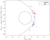 |
Fig. 5 Location of the bow shock crossings for all events. The red crosses show MEX crossings, and the blue crosses show MAVEN crossings. |
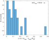 |
Fig. 6 Histogram of Δd = |dmav − dmex| for all 20 events. |
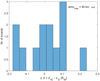 |
Fig. 7 Histogram of Δd = d+E − d−E for the 11 events where the spacecraft crossed the bow shock on opposing E hemispheres. |
3.2.3 Asymmetry with respect to the convective electric field, Esw
This section describes 11 events in which each spacecraft crossed the bow shock on different E hemispheres. The average time difference between the crossings was 16.3 minutes, the largest time difference was 40.8 minutes, and the shortest time difference was 1.9 minutes. In Figure 8 we show the locations of the bow shock crossings. There is an even spread of MAVEN and MEX crossings on the two hemispheres, with MAVEN and MEX being in the + E hemisphere five and six times, respectively. Figure 7 shows a histogram of Δd = d+E − d−E. There is no clear trend toward either E hemisphere being farther away from the planet. The average Δd for all events was 0.006 RM, which is insignificant considering that one standard deviation, 1σ, is 0.12 RM. The average distances d from the bow shock model were 0.118 and 0.112 RM for the +E and −E hemisphere, respectively. The values d+E, d−E, Δd = d+E − d−E, the time difference, the mean values and 1σ, which spacecraft was in the + E hemisphere, and upstream MA, Pdyn, and the solar EUV flux are listed in Table A.2 in the Appendix.
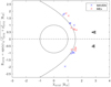 |
Fig. 8 Location of the bow shock crossings for the events of opposing E hemispheres. The red crosses show MEX crossings, and the blue crosses show MAVEN crossings. |
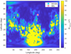 |
Fig. 9 Projection of the position of MAVEN and MEX on Mars during a bow shock crossing. The blue and red circles show the projected position for MAVEN and MEX, respectively. |
3.2.4 Asymmetry with respect to the Martian crustal fields
The position of the spacecraft at the time of the crossing was projected onto the surface to show the longitude and latitude of the spacecraft on Mars. In this way, we determined whether the spacecraft crossed the bow shock over a region of high or low crustal fields. An example is given in Figure 9, where MAVEN is represented by a turqoise dot, and MEX is represented by a pink dot. MAVEN crossed the bow shock over a region of strong crustal fields, and MEX crossed over a region of weak crustal fields. The distance to the bow shock model for this specific event was 0.045 RM for MAVEN and 0.272 RM for MEX, giving Δd = dHiɡhCF − dLowCF = -0.228 RM. This data set also included 11 events with some overlap of events from the previous section. The average time difference for these events was 8.6 minutes, the longest time separation was 18.7 minutes, and the shortest time separation was 1.9 minutes. Similar to Section 3.2.3, the locations of the bow shock crossings are shown in Figure 10, which shows that the distribution of MEX and MAVEN crossings over the dayside is quite equal.
In Figure 11 we show a histogram of Δd = dHiɡhCF − dLowCF. Similar to Figure 7, there is no clear trend for regions with a smaller or larger crustal field strength to cause the bow shock to extend farther away from the planet. The mean of Δd for the 11 events was -0.016 RM, and the standard deviation was 0.186 RM.
The asymmetry that would be expected would be for a positive mean because regions with a large crustal field strength are expected to push the bow shock out from the planet. As in the previous section, the values for the means and standard deviations for dHiɡhCF and dLowCF, time differences, which spacecraft was over a region with a large crustal field strength, and upstream MA, Pdyn, and solar EUV flux are listed in Table A.3 in the Appendix.
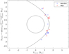 |
Fig. 10 Location of the bow shock crossings for events in a region with a large or small crustal field strength. The red crosses show MEX crossings, and the blue crosses show MAVEN crossings. |
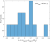 |
Fig. 11 Histogram of Δ d = dHiɡhCF − dLowCF for the 11 events where one spacecraft crossed over a region of strong crustal fields, and one spacecraft crossed over a region of weak crustal fields. |
4 Discussion
As noted in the introduction, several factors influence the position of the bow shock. Whether these factors might also yield a false perception of the asymmetry deserves some consideration. Such an error might occur when one of the important drivers of the bow shock location changed during our measurements, so that it was different when the spacecraft was in the solar wind compared to when it was in the magnetosheath in our singlespacecraft method, or when a driver changed in between bow shock crossings in the dual-spacecraft method. The solar EUV flux measured by the EUV monitor onboard MAVEN shows no appreciable changes on the timescale of minutes, which is relevant to our single-spacecraft method. Even in the counterfactual case that a significant change would have occurred during one of the events, the timescale of minutes is much faster than what is required for a change in EUV flux to change the ionosphere and in turn affect the bow shock. For Earth, Vaishnav et al. (2021) found that the ionospheric response is delayed by ∼17 h, and while Mars could have a somewhat different delay, the ionization timescales are much slower than the timescales of minutes on which the magnetic field reverses. Similarly, the time separation on the scale of minutes in the dual-spacecraft method is unlikely to allow significant change in terms of the ionization of the magnetosheath.
In the same way, the Martian crustal fields cannot affect the results of the single-spacecraft method, as the spacecraft position with respect to the crustal field does not change significantly on the timescale of minutes for the spacecraft motion or the planetary rotation. Furthermore, no significant asymmetry with regard to crustal fields was found in the dual-spacecraft study, even when one spacecraft was directly above the region of strong crustal fields and the other spacecraft was not.
Another possible influence is whether the spacecraft observes a quasi-parallel or quasi-perpendicular bow shock. This might affect the bow shock stand-off distance. We computed the angle between the shock normal and the IMF, as measured when MAVEN was in the solar wind, and we include this angle in Table 1. If this effect had influenced our result, there should be a systematic occurrence of either the quasi-parallel or quasi-perpendicular shock for the cases when we find the magnetosheath in the −E hemisphere. No such correlation can be seen in Table 1. In the dual-spacecraft method, the majority of the crossings occurred for θbn >45° for both spacecraft, which reduces the likelihood that θbn causes the asymmetry.
The dynamic pressure pdyn and Mach number MA were treated in the same way, and in this case, the variations in these values did not systematically follow the observations of in which hemisphere the magnetosheath was found either. However, the change in the IMF direction might be correlated to a change in a different solar wind property, and this might cause the change in the bow shock position. One of these correlations was examined by Maggiolo et al. (2017), namely the correlation between the solar wind speed and the individual Bx, By, and Bz components of the IMF. They found no significant correlation. Thus, we hold this possibility as unlikely, but admittedly, it cannot be verified by the single-spacecraft method, as the solar wind properties are not monitored when MAVEN is in the magnetosheath.
We first used a single-spacecraft method, wherein MAVEN data were studied during a change in the IMF orientation. Based on this method, we can say with a 94% degree of confidence that the bow shock is asymmetric. The bow shock is farther from the x-axis in the −E hemisphere than in the + E hemisphere. The method indicates asymmetry, but is unable to quantify this asymmetry. Then we applied a two-spacecraft method, with which we were able to quantify the asymmetry. The results did not indicate a significant asymmetry due to the Esw. The variation was large, 0.12 RM, meaning that there was large spread in Δd for the events, but the low mean value, 0.006 RM, shows that Esw is not the primary cause for this asymmetry. The difference in the results between the single- and dual-spacecraft method could indicate that if there is an asymmetry with respect to Esw, it could be short lived and cause an asymmetry during a change in the IMF orientation, but the asymmetry disappears after a few minutes, as per the time difference in the dual-spacecraft section.
We found similar results when the data set was divided into high and low crustal field regions. The average was very small, at −0.016 RM, indicating that crustal fields were not a primary reason for asymmetry either. When we studied the asymmetry regardless of the cause, the variations in the bow shock location for opposite hemispheres were large. The mean Δd was 0.13 RM, corresponding to 7.8% of the scale length, Ls.
One way of validating the method was to study the solar wind conditions for the events. In the dual-spacecraft study, MAVEN passed in 19 out of 20 cases from the solar wind to the magnetosheath, and MEX moved in the opposite direction, from the magnetosheath to the solar wind. In these cases, MAVEN provided information on the solar wind conditions up until the crossing. If the conditions were calm, the probability that the conditions for MAVEN and MEX crossings are also mild increases. For example, in Fig. 3, MAVEN is shown to observe the mostly calm solar wind for 15 minutes before it approaches the shock region. In the majority of the events, the solar wind conditions are calm, indicating that changes in the distance are more unlikely to be related to the solar wind changes. In some events, the solar wind is somewhat disturbed, raising the possibility that conditions changed between the two spacecraft crossings.
We further validated the method to investigate whether Δd increased with increasing time between the bow shock crossings of MAVEN and MEX, Δt. This is not the case; Δd is spread evenly over Δt (figure not shown). Similarly, we separately investigated the histograms of Δd for MAVEN and MEX to ensure that no spacecraft observed systematically higher values of Δd than the other, which might imply a bias or error by one set of measurements. However, in the same way as for the time difference, there was an even spread of Δd for the spacecraft sets. This means that there probably was no bias for either spacecraft.
The nature and causes of the spatial variability might have several reasons. As indicated by the findings of this study, the convective electric field might cause asymmetries on shorter timescales. Previous simulations have indicated that there is large-scale structuring of the bow shock and the magnetosheath in the + E hemisphere (Kallio et al. 2006), indicating that fluctuations and wave phenomena can cause short-timescale asymmetries. Beyond the convective electric field, the orientation of the IMF is known to affect the bow shock location, with quasi-perpendicular shocks located farther from the planet than quasi-parallel shocks. Garnier et al. (2022a) studied the terminator altitude of the Martian bow shock for different θbn and found a statistically significant altitude increase for increasing θbn.
Shock reformation might also contribute to the observed asymmetry. Madanian et al. (2020) observed a reformation of the Martian bow shock, in which waves ahead of the shock were steepened and became the new shock front (Krasnoselskikh et al. 2002, 2013). The bow shock might be re-formed between the observed crossings, which might affect the location of the bow shock. The shock reformation is thought to occur on timescales of the ion gyroperiod, which in the event studied by Madanian et al. (2020) was 24.2 s. This is well within the time separation of the data in this study.
Local phenomena might also contribute to the variability in the bow shock location. Johlander et al. (2016) studied ripples of the quasi-perpendicular bow shock at Earth with the Magnetospheric Multiscale (MMS) Mission. The ripples in the observed events caused amplitude differences of up to 30 km, which is smaller by an order of magnitude than the average ∼300 km amplitude difference seen in this study. Temporal variations also need to be taken into account. Because we lack a solar wind monitor and because there is no magnetometer on MEX, we cannot determine a difference in the solar wind conditions between each pair of crossings. Cheng et al. (2023) conducted a dual-spacecraft study and found that variations in the solar wind conditions caused a response in the Martian bow shock on timescales shorter than one minute.
5 Conclusion
This study used two methods. The first was a single-spacecraft study, in which a change in the IMF direction was used to study a shift in the magnetosheath hemisphere in the MSE coordinate system. The results indicated that there was an asymmetry in between the −E and + E hemispheres, but the single-spacecraft method could not quantify this asymmetry. The second method was a dual-spacecraft method, in which near simultaneous bow shock crossings by MAVEN and MEX were studied. In this method, the observed bow shock crossings were compared to a model, and the difference in the distance to the bow shock model Δd was calculated as a measure of asymmetry. The method showed a strong asymmetry of the Martian bow shock, but was unable to determine a correlation with the convective electric field direction or with crustal fields.
Future research should include a larger data set when it becomes available. The upcoming EscaPADE mission at Mars (Lillis et al. 2022) is a dual-spacecraft mission. In its final science orbits, the two spacecraft travel nearly in phase, perpendicular to each other, which would hopefully facilitate a data set of near simultaneous bow shock crossings.
This study has shown that there is a significant asymmetry at the Martian bow shock, and that these asymmetries on timescales of individual observations are stronger than the average asymmetries. This indicates the dynamic and likely highly kinetic nature of the Martian system.
Acknowledgements
All MAVEN data are publicly available through the Planetary Data System <https://pds-ppi.igpp.ucla.edu/mission/MAVEN/> (NASA 2023). This work was funded by the Swedish National Space Agency (SNSA, projects 2023-00208 and 194/19).
Appendix A Additional tables
Table containing information regarding all the dual-spacecraft bow shock crossings.
Table containing information regarding the dual-spacecraft bow shock crossings where the spacecraft were located in different E hemispheres.
Table containing information regarding the dual-spacecraft bow shock crossings where one spacecraft was located over a region of strong crustal fields, and one spacecraft over a region of weak crustal fields.
References
- Barabash, S., Lundin, R., Andersson, H., et al. 2006, Space Sci. Rev., 126, 113 [NASA ADS] [CrossRef] [Google Scholar]
- Bertucci, C., Duru, F., Edberg, N., et al. 2011, Space Sci. Rev., 162, 113 [Google Scholar]
- Brain, D. A., Bagenal, F., Acuña, M. H., & Connerney, J. E. P. 2003, J. Geophys. Res.: Space Physics, 108, A12 [CrossRef] [Google Scholar]
- Cheng, L., Lillis, R., Wang, Y., et al. 2023, Geophys. Res. Lett., 50, e2023GL104769 [NASA ADS] [CrossRef] [Google Scholar]
- Chicarro, A., Martin, P., & Trautner, R. 2004, Mars Express: The Scientific Payload, ed. A. Wilson, scientific coordination: A. Chicarro. ESA SP-1240 (Noordwijk, Netherlands: ESA Publications Division), 3 [Google Scholar]
- Connerney, J. E. P., Espley, J., Lawton, P., et al. 2015, Space Sci. Rev., 195, 257 [NASA ADS] [CrossRef] [Google Scholar]
- Dong, Y., Fang, X., Brain, D. A., et al. 2015, Geophys. Res. Lett., 42, 8942 [NASA ADS] [CrossRef] [Google Scholar]
- Dubinin, E., Sauer, K., Baumgärtel, K., & Lundin, R. 1997, ASR, 20, 149 [Google Scholar]
- Edberg, N. J. T., Lester, M., Cowley, S. W. H., & Eriksson, A. I. 2008, J. Geophys. Res.: Space Phys., 113, A08206 [NASA ADS] [CrossRef] [Google Scholar]
- Edberg, N. J. T., Brain, D. A., Lester, M., et al. 2009, ANGEO, 27, 3537 [NASA ADS] [CrossRef] [Google Scholar]
- Edberg, N. J. T., Lester, M., Cowley, S. W. H., et al. 2010, J. Geophys. Res.: Space Phys., 115, A07203 [NASA ADS] [CrossRef] [Google Scholar]
- Eparvier, F., Chamberlin, P., Woods, T., & Thiemann, E. 2015, Space Sci. Rev., 195, 293 [NASA ADS] [CrossRef] [Google Scholar]
- Fang, X., Liemohn, M. W., Nagy, A. F., et al. 2008, J. Geophys. Res.: Space Phys., 113, A02210 [NASA ADS] [Google Scholar]
- Fang, X., Ma, Y., Masunaga, K., et al. 2017, J. Geophys. Res.: Space Phys., 122, 4117 [NASA ADS] [CrossRef] [Google Scholar]
- Garnier, P., Jacquey, C., Gendre, X., et al. 2022a, J. Geophys. Res.: Space Phys., 127, e2021JA030147 [CrossRef] [Google Scholar]
- Garnier, P., Jacquey, C., Gendre, X., et al. 2022b, J. Geophys. Res.: Space Physics, 127, e2021JA030146 [CrossRef] [Google Scholar]
- Goetz, C., Gunell, H., Johansson, F., et al. 2021, ANGEO, 39, 379 [NASA ADS] [CrossRef] [Google Scholar]
- Gruesbeck, J. R., Espley, J. R., Connerney, J. E. P., et al. 2018, J. Geophys. Res. (Space Phys.), 123, 4542 [NASA ADS] [CrossRef] [Google Scholar]
- Gunell, H., Goetz, C., Simon Wedlund, C., et al. 2018, A&A, 619, L2 [NASA ADS] [CrossRef] [EDP Sciences] [Google Scholar]
- Halekas, J. S., Taylor, E. R., Dalton, G., et al. 2015, Space Sci. Rev., 195, 125 [CrossRef] [Google Scholar]
- Halekas, J. S., Ruhunusiri, S., Harada, Y., et al. 2017, J. Geophys. Res. (Space Phys.), 122, 547 [NASA ADS] [CrossRef] [Google Scholar]
- Hall, B. E. S., Sánchez-Cano, B., Wild, J. A., Lester, M., & Holmström, M. 2019, J. Geophys. Res.: Space Phys., 124, 4761 [NASA ADS] [CrossRef] [Google Scholar]
- Jakosky, B. M., Lin, R. P., Grebowsky, J. M., et al. 2015, Space Sci. Rev., 195, 3 [CrossRef] [Google Scholar]
- Johlander, A., Schwartz, S., Vaivads, A., et al. 2016, PRL, 117, 165101 [NASA ADS] [CrossRef] [Google Scholar]
- Kallio, E., Fedorov, A., Budnik, E., et al. 2006, Icarus, 182, 350 [NASA ADS] [CrossRef] [Google Scholar]
- Krasnoselskikh, V., Lembège, B., Savoini, P., & Lobzin, V. 2002, Phys. Plasmas, 9, 1192 [CrossRef] [Google Scholar]
- Krasnoselskikh, V., Balikhin, M., Walker, S., et al. 2013, Space Sci. Rev., 178, 535 [NASA ADS] [CrossRef] [Google Scholar]
- Larkin, C. J., Lundén, V., Schulz, L., et al. 2024, ASR, 73, 3235 [Google Scholar]
- Lillis, R. J., Mitchell, D., Montabone, L., et al. 2021, PSJ, 2, 211 [NASA ADS] [Google Scholar]
- Lillis, R. J., Curry, S. M., Ma, Y. J., et al. 2022, in LPI Contributions, 2678, 1135 [NASA ADS] [Google Scholar]
- Luhmann, J., Ledvina, S., & Russell, C. 2004, ASR, 33, 1905 [Google Scholar]
- Madanian, H., Schwartz, S. J., Halekas, J. S., & Wilson III, L. B. 2020, Geophys. Res. Lett., 47, e2020GL088309 [CrossRef] [Google Scholar]
- Maggiolo, R., Hamrin, M., Keyser, J. D., et al. 2017, J. Geophys. Res. (Space Phys.), 122, 11109 [Google Scholar]
- Mazelle, C., Winterhalter, D., Sauer, K., et al. 2004, Space Sci. Rev., 111, 115 [NASA ADS] [CrossRef] [Google Scholar]
- Mitchell, D. L., Mazelle, C., Sauvaud, J.-A., et al. 2016, Space Sci. Rev., 200, 495 [NASA ADS] [CrossRef] [Google Scholar]
- Möhlmann, D., Sauer, K., Roatsch, T., Schwingenschuh, K., & Kurths, J. 1992, ASR, 12, 221 [Google Scholar]
- NASA 2023, PDS, https://pds-ppi.igpp.ucla.edu/mission/MAVEN [Google Scholar]
- NOAA 2023, Solar Cycle Progression | NOAA / NWS Space Weather Prediction Center, https://www.swpc.noaa.gov/products/solar-cycle-progression [Google Scholar]
- Ramstad, R., Barabash, S., Futaana, Y., & Holmström, M. 2017, J. Geophys. Res.: Space Phys., 122, 7279 [NASA ADS] [CrossRef] [Google Scholar]
- Romanelli, N., DiBraccio, G., Modolo, R., et al. 2019, Geophys. Res. Lett., 46, 10977 [NASA ADS] [CrossRef] [Google Scholar]
- Sanchez-Cano, B., Opgenoorth, H., Leblanc, F., Andrews, D., & Lester, M. 2022, 44th COSPAR Scientific Assembly, 16–24 July, 44, 421 [Google Scholar]
- Schwingenschuh, K., Riedler, W., Lichtenegger, H., et al. 1990, Geophys. Res. Lett., 17, 889 [NASA ADS] [CrossRef] [Google Scholar]
- Schwingenschuh, K., Riedler, W., Zhang, T.-L., et al. 1992, ASR, 12, 213 [Google Scholar]
- Slavin, J. A., & Holzer, R. E. 1982, J. Geophys. Res.: Solid Earth, 87, 10285 [NASA ADS] [CrossRef] [Google Scholar]
- Thiemann, E. M., Chamberlin, P. C., Eparvier, F. G., et al. 2017, J. Geophys. Res.: Space Physics, 122, 2748 [NASA ADS] [CrossRef] [Google Scholar]
- Trotignon, J., Grard, R., & Skalsky, A. 1993, P&SS, 41, 189 [NASA ADS] [CrossRef] [Google Scholar]
- Trotignon, J., Mazelle, C., Bertucci, C., & Acuña, M. 2006, P&SS, 54, 357 [NASA ADS] [CrossRef] [Google Scholar]
- Tsurutani, B. T., Echer, E., Guarnieri, F. L., & Kozyra, J. U. 2008, Geophys. Res. Lett., 35, L06S05 [NASA ADS] [CrossRef] [Google Scholar]
- Vaisberg, O., Ermakov, V., Shuvalov, S., et al. 2018, J. Geophys. Res.: Space Phys., 123, 2679 [NASA ADS] [CrossRef] [Google Scholar]
- Vaishnav, R., Schmölter, E., Jacobi, C., Berdermann, J., & Codrescu, M. 2021, ANGEO, 39, 341 [NASA ADS] [CrossRef] [Google Scholar]
- Vignes, D., Acuña, M. H., Connerney, J. E. P., et al. 2002, Geophys. Res. Lett., 29, 42 [CrossRef] [Google Scholar]
- Withers, P., & Jakosky, B. M. 2017, J. Geophys. Res.: Space Phys., 122, 802 [NASA ADS] [CrossRef] [Google Scholar]
- Yi, Y., Kim, E.-J., Kim, Y.-H., & Kim, J. 1999, JASS, 16, 139 [NASA ADS] [Google Scholar]
- Zhang, T.-L., Schwingenschuh, K., Russell, C. T., & Luhmann, J. G. 1991, Geophys. Res. Lett., 18, 127 [NASA ADS] [CrossRef] [Google Scholar]
- Zhao, D., Guo, J., Huang, H., et al. 2021, AJ, 923, 4 [NASA ADS] [Google Scholar]
All Tables
Table containing information regarding all the dual-spacecraft bow shock crossings.
Table containing information regarding the dual-spacecraft bow shock crossings where the spacecraft were located in different E hemispheres.
Table containing information regarding the dual-spacecraft bow shock crossings where one spacecraft was located over a region of strong crustal fields, and one spacecraft over a region of weak crustal fields.
All Figures
|
Fig. 1 Single-spacecraft observation. Example from 7 October 2015, showing a case when magnetosheath plasma was found in the −E hemisphere. (a) Logarithm of the differential energy flux of the ions in units of eV/(cm2s sr eV), (b) logarithm of the differential energy flux of the electrons in units of eV /(cm2s sr eV), (c) normalized integrated electron energy flux Fe, (d) magnetic flux density components, (e) normalized zMSE coordinate cos θ, (f) Fe (color-coded) at the positions of the observation in the yMSE − zMSE plane, and (g) Fe (color-coded) at the positions of the observation in the xMSE− zMSE plane. The magnetosheath is characterized by a higher electron flux Fe, as shown in panels c, f, and g. The −E hemisphere corresponds to cos θ < 0. |
| In the text | |
|
Fig. 2 Single-spacecraft observation. Example from 10 March 2018, showing a case when magnetosheath plasma was found in the +E hemisphere. (a) Logarithm of the differential energy flux of the ions in units of eV/(cm2s sr eV), (b) logarithm of the differential energy flux of the electrons in units of eV /(cm2s sr eV), (c) normalized integrated electron energy flux Fe, (d) magnetic flux density components, (e) normalized zMSE coordinate cos θ, (f) Fe (color-coded) at the positions of observation in the yMSE–zMSE plane, and (g) Fe (color-coded) at the positions of observation in the xMSE–zMSE plane. The magnetosheath is characterized by a higher electron flux Fe, as shown in panels c, f, and g. The −E hemisphere corresponds to cos θ < 0. |
| In the text | |
|
Fig. 3 Data from an example event where MAVEN and MEX crossed the bow shock within 10 minutes of each other. The left side shows MAVEN data, and the panels show (a) the electron energy spectrogram, (b) the ion energy spectrogram, (c) the magnetic field, (d) the ion density, (e) the ion bulk velocity, and (f) the spacecraft position. The right plot shows MEX data, and the panels show (g) the electron energy spectrogram, (h) the ion energy spectrogram, (i) the proton density, (j) the proton velocity, and (k) the spacecraft position. The arrows above the two figures indicate the regions through which the spacecraft traveled. The vertical black line shows the manually chosen bow shock crossing. All data are given in the MSO coordinate system. |
| In the text | |
|
Fig. 4 Calculation of Δd. The blue and red crosses indicate the observed crossings of the two spacecraft, d1 and d2 are distances to the modeled bow shock, and Δd is the difference between these distances. The distances are exaggerated for clarity. |
| In the text | |
|
Fig. 5 Location of the bow shock crossings for all events. The red crosses show MEX crossings, and the blue crosses show MAVEN crossings. |
| In the text | |
|
Fig. 6 Histogram of Δd = |dmav − dmex| for all 20 events. |
| In the text | |
|
Fig. 7 Histogram of Δd = d+E − d−E for the 11 events where the spacecraft crossed the bow shock on opposing E hemispheres. |
| In the text | |
|
Fig. 8 Location of the bow shock crossings for the events of opposing E hemispheres. The red crosses show MEX crossings, and the blue crosses show MAVEN crossings. |
| In the text | |
|
Fig. 9 Projection of the position of MAVEN and MEX on Mars during a bow shock crossing. The blue and red circles show the projected position for MAVEN and MEX, respectively. |
| In the text | |
|
Fig. 10 Location of the bow shock crossings for events in a region with a large or small crustal field strength. The red crosses show MEX crossings, and the blue crosses show MAVEN crossings. |
| In the text | |
|
Fig. 11 Histogram of Δ d = dHiɡhCF − dLowCF for the 11 events where one spacecraft crossed over a region of strong crustal fields, and one spacecraft crossed over a region of weak crustal fields. |
| In the text | |
Current usage metrics show cumulative count of Article Views (full-text article views including HTML views, PDF and ePub downloads, according to the available data) and Abstracts Views on Vision4Press platform.
Data correspond to usage on the plateform after 2015. The current usage metrics is available 48-96 hours after online publication and is updated daily on week days.
Initial download of the metrics may take a while.