| Issue |
A&A
Volume 693, January 2025
|
|
|---|---|---|
| Article Number | A78 | |
| Number of page(s) | 6 | |
| Section | Planets, planetary systems, and small bodies | |
| DOI | https://doi.org/10.1051/0004-6361/202451322 | |
| Published online | 03 January 2025 | |
Observation of discontinuities accompanied by interplanetary shock within the Martian magnetosheath
1
Institute for Frontiers in Astronomy and Astrophysics, Beijing Normal University,
Beijing
102206,
PR
China
2
Planetary and Space Physics Group, School of Physics and Astronomy, Beijing Normal University,
Beijing
100875,
PR
China
★★ Corresponding author; This email address is being protected from spambots. You need JavaScript enabled to view it.
; This email address is being protected from spambots. You need JavaScript enabled to view it.
Received:
1
July
2024
Accepted:
2
December
2024
Abstract
As fast forward interplanetary (IP) shocks travel outward in the IP medium, they might encounter planetary bow shocks (BSs) and then propagate into the magnetosheath. The interaction of an IP shock with a BS could create a new discontinuity, which has been predicted by theory and simulations, and commonly observed at Earth. Nevertheless, it is still uncertain whether such a phenomenon occurs at unmagnetized planets like Mars. Here, we present the first experimental observation of a discontinuity-like structure that follows a transmitted IP shock within the Martian magnetosheath. This event was recorded by the MAVEN spacecraft on March 3, 2015. The comparison of spacecraft measurements with theoretical studies indicates that the discontinuity-like structure is a compound structure in nature, composed of the slow expansion wave, contact discontinuity, and slow shock, launched by the interaction of a fast IP shock with the Martian BS. The results shed light on the similarities between magnetized and unmagnetized planets in response to the passage of IP shocks.
Key words: plasmas / methods: observational / planets and satellites: individual: Mars
Co-first author. The authors contributed equally to this work.
© The Authors 2025
 Open Access article, published by EDP Sciences, under the terms of the Creative Commons Attribution License (https://creativecommons.org/licenses/by/4.0), which permits unrestricted use, distribution, and reproduction in any medium, provided the original work is properly cited.
This article is published in open access under the Subscribe to Open model. This email address is being protected from spambots. You need JavaScript enabled to view it. to support open access publication.
1 Introduction
When the supersonic solar wind interacts with a planetary obstacle, a bow shock (BS) forms in front of the planetary obstacle. The BS serves to slow down the flowing solar wind from supersonic to subsonic and to heat it. The nature of the obstacle can be very different, depending upon whether the planet has a sufficiently large intrinsic magnetic field or a dense enough ionosphere (Barabash 2012). In the case in which the planet posseses a strong dipole magnetic field (e.g., Mercury, Earth, and all giant planets), the dipole field is subject to the solar wind flow, resulting in the formation of a cavity called the magnetosphere (Blanco-Cano et al. 2004). The shocked solar wind flow is deflected around the magnetosphere by the planetary magnetic field and the currents induced by the solar wind interaction (Ganushkina et al. 2018). The boundary between the magnetosphere and the surrounding solar wind is the magnetopause. The region between the BS and the magnetopause is the magnetosheath. In the case in which the planet has no intrinsic global magnetic dipole and but a well-developed ionosphere (e.g., Venus and Mars), the ionosphere presents the primary obstacle to the solar wind flow. The resulting interaction induces electric currents in the ionosphere, which create magnetic field and then provide sufficient magnetic pressure to slow and deflect the solar wind, leading to the formation of an induced magnetosphere (Intriligator & Smith 1979; Ramstad et al. 2020). It should be emphasized here that Mars possesses a remnant crustal magnetic field located mostly in the southern hemisphere (Acuna et al. 1998, 1999), which adds a complex obstacle to the solar wind flow. The transition between the interplanetary (IP) magnetic field and induced magnetic field dominance is referred to as the induced magnetosphere boundary, analogous to the magnetopause in intrinsic magnetospheres. The region between the BS and the induced magnetosphere boundary is the magnetosheath.
The size of the planetary obstacle largely determines the size of the BS relative to the planet. Mars is much smaller and located at a larger heliocentric distance in comparison to Earth. The BS at Mars is correspondingly smaller than the one at Earth. The Earth’s magnetosheath has a scale much greater than solar wind ion scales. In contrast, the Martian magnetosheath is of a smaller spatial extent, with a thickness that is comparable to the gyroradius of the protons (normally about 1000 km) and a lateral scale only an order of magnitude greater (Halekas et al. 2017a). Specifically, at the subsolar region, the thickness of the Martian magnetosheath is about 0.38 RM (RM ~ 3400 km is the Mars radius); at the terminator region, it is about 2500 km (Dubinin et al. 1993, 1995). The flowing solar wind could not be fully thermalized in a much shorter distance downstream from the Martian BS (Moses et al. 1988). In addition to the small size, the Martian magnetosheath has other complicating factors that are not present at Earth. For instance, owing to the weak Martian gravity, the Martian BS and magnetosheath is immersed in a dense and extended neutral exosphere. Both heavy ions (e.g., O+) and cold protons of exospheric origin can modify the overall ion dynamics within the magnetosheath. Significant mass-loading of pickup ions takes place within the magnetosheath. Moreover, the BS and the magnetosheath structure could be further complicated by the presence of strong crustal magnetic fields (Brain et al. 2005).
As fast forward (FF) IP shocks travel outward in the IP medium, they might encounter planetary BSs. In theory, the Rankine-Hugoniot jump conditions on discontinuity given by the contact line of two interacting shock fronts are not satisfied. This discontinuity splits up immediately into an ensemble of other discontinuities or self-similar waves (Akhiezer 1975). The solution could be a combination of several discontinuities and rarefaction waves. Numerous simulation and observational studies have been devoted to the interaction of an IP shock with the Earth’s BS. It has been established that a FF IP shock passing through the Earth’s BS can create a new discontinuity that follows the modified IP shock (often referred to as the transmitted IP shock) (Grib et al. 1979; Zhuang et al. 1981; Grib 1982; Yan & Lee 1996; Samsonov et al. 2006; Šafránková et al. 2007; Pallocchia et al. 2010; Samsonov 2011; Zhang et al. 2012). This newly created discontinuity is actually a combination of several discontinuities, typically including a forward slow expansion wave, a contact discontinuity, and a reversed slow shock (Yan & Lee 1996; Samsonov et al. 2006). In the plasma frame, the slow expansion wave propagates away from the BS toward the magnetopause, the slow shock propagates toward the BS, and the contact discontinuity does not propagate. Since the plasma flow speed is locally below the fast-mode phase speed and above the slow-mode phase speed, all of these discontinuities or waves travel toward the magnetopause (Yan & Lee 1996). Their propagation speeds are quite similar, and thus they cannot be clearly distinguished in the spacecraft data or in results of numerical simulations (Samsonov et al. 2006), so naturally they are identified as just one discontinuity (Yan & Lee 1996; Samsonov et al. 2006; Šafránková et al. 2007; Pallocchia et al. 2010; Zhang et al. 2012). Immediately after the BS crossing, the IP shock experiences a deceleration in the magnetosheath; that is, the transmitted shock is slowed down with respect to the original IP shock (Koval et al. 2005, 2006; Samsonov et al. 2006; Pallocchia et al. 2010). The BS begins an inward (earthward) motion and then an outward motion, giving rise to a “trough” structure on the BS surface, which proceeds along the BS surface with a slightly smaller speed than that of the original IP shock propagating in the IP medium. After propagation through the magnetosheath, the transmitted IP shock impinges on the magnetopause, resulting in a rarefaction wave that propagates toward the BS. At the same time, the magnetopause experiences an inward motion (Samsonov et al. 2006; Šafránková et al. 2007; Pallocchia 2013).
The scenario for a FF shock passing through the BS at Mars may share some similarities with that at Earth, despite general differences between Mars and Earth mentioned above. As yet, the similarities remain to be verified observationally. The Mars Atmosphere and Volatile Evolution (MAVEN) spacecraft was launched in November 2013 and arrived at Mars in September 2014. It is in an elliptical orbit with a periapsis altitude of ~150 km and an apoapsis altitude of ~6500 km, and precesses in both local time and longitude (Jakosky et al. 2015b). The measurements by the MAVEN spacecraft provide an opportunity to investigate the IP shock interaction with the Martian BS with simultaneous monitoring of plasma and the magnetic field. Our preliminary efforts have been made toward the identification of transmitted IP shocks propagating through the Martian magnetosheath. The results indicate that only three transmitted IP shocks were encountered by MAVEN inside the magnetosheath during the period from October 2014 to February 2023. They occurred around 18:17:53 UT on March 3, 2015, around 02:52:00 UT on September 13, 2017, and around 08:48:14 UT on May 9, 2019, respectively. Here, we are primarily interested in the transmitted IP shock event on March 3, 2015. It is a quasi-perpendicular fast shock and propagates toward the Mars with a relatively high speed. About 41 seconds after the shock arrival, a discontinuity-like structure was detected. The discontinuity-like structure can be explained as a compound structure composed of the slow expansion wave, contact discontinuity, and slow shock that are created by the interaction of the IP shock with the Martian BS. This paper provides a report on this event.
2 MAVEN data
The MAVEN spacecraft carries nine sensors that measure the plasma and neutral environment at Mars. The primary data used in this work were collected from three instruments on board MAVEN: the Solar Wind Ion Analyzer (SWIA; Halekas et al. 2015), the Solar Wind Electron Analyzer (SWEA; Mitchell et al. 2016), and the Magnetometer (MAG; Connerney et al. 2015). SWIA is a toroidal energy analyzer with electrostatic deflectors that measures ions over a broad 360° × 90° field of view. It provides 3D velocity distributions of ions over an energy range from 25 eV to 25 keV with a 14.5% energy resolution. SWIA does not discriminate between ion species. The on-board proton moments (density, velocity, and temperature) can be derived from the Coarse 3D data under the assumption that all ions are protons. However, it is worth noting that even a small heavy ion population leads to an artificially high temperature moment due to their higher energy per charge. On-board-computed ion energy spectra (1D ion energy spectra) with a 4 s time resolution and Coarse ion energy spectra computed on the ground from the Coarse 3D data with a 32 s time resolution are utilized. In the Coarse data, each of the two neighboring energy bins are grouped together, resulting in 48 energy bins. The 10 fine anodes are binned in groups of five, resulting in two 22.5° bins in the solar wind direction, which in addition to the 14 coarse anodes create a total of 16 azimuth bins of 22.5°, and there are four elevation bins with a resolution of 22.5°. SWEA measures the energy and angular distributions of 3–4600 eV electrons, providing the electron moments and electron energy spectra. The magnetic field data are from MAG with a cadence of 1 s. The MAVEN data are utilized in the Mars Solar Orbital (MSO) coordinate system, where X is aligned from Mars to the Sun, Z points to the north ecliptic pole, and Y completes the right-handed system.
3 Observations of shock and discontinuity
Figure 1 illustrates the MAVEN trajectory corresponding to orbit 822 on March 3, 2015, projected onto the principal planes of the MSO coordinate system and in cylindrical coordinates. MAVEN passed periapsis (~152.2 km altitude) around 16:08:21 UT on the dusk side, and reached apoapsis (~6227.1 km altitude) around 18:23:36 UT on the dawn side and in the southern magnetosheath. We note that orbit 822 did not extend out of the Martian BS. In this study, we focus on the orbit spanning 18:08-18:28 UT surrounding the apoapsis. The plasma and magnetic field observations during this time span are shown in Figure 2. A forward shock at 18:17:53 UT is clearly visible and is indicated by the vertical dashed blue line. It is characterized by a sudden increase in the magnetic field magnitude, abrupt increases in ion density and velocity, as well as significant broadening of ion and electron energy spectra across the shock from upstream to downstream. An overshoot is present in the magnetic field profile just downstream of the shock. This shock has been unambiguously identified as a transmitted IP shock propagating through the magnetosheath. It was launched by the interaction of a FF IP shock (not recorded in the upstream solar wind region) with the Martian BS (He et al. 2023). The IP shock was driven by an IP coronal mass ejection (ICME), passing through Mars on March 3–4, 2015 (Jakosky et al. 2015a; Thampi et al. 2018), and thus can be reasonably classified as a FF shock. It is worth mentioning here that the most frequently observed shocks driven by ICMEs are fast shocks (see, Huang et al. 2021).
We have made an effort to estimate several key shock parameters, including the shock normal, n, the shock angle, θBn, the shock velocity, Vsh, and the shock strength. To avoid the large disturbance of magnetic field direction in the interval of 2 minutes before the shock crossing, the upstream interval was chosen as 18:11:53–18:15:53 UT. Similarly, to avoid a discontinuity-like structure occurred around 18:18:34 UT (described in detail later), the downstream interval was chosen as 18:18:00–18:18:25 UT.
The shock normal pointing upstream was calculated by
![Mathematical equation: $\[\boldsymbol{n}= \pm \frac{\left(\boldsymbol{B}^{down}-\boldsymbol{B}^{up}\right) \times\left(\left(\boldsymbol{B}^{down}-\boldsymbol{B}^{up}\right) \times\left(\boldsymbol{V}^{down}-\boldsymbol{V}^{u p}\right)\right)}{\left|\left(\boldsymbol{B}^{down}-\boldsymbol{B}^{up}\right) \times\left(\left(\boldsymbol{B}^{down}-\boldsymbol{B}^{up}\right) \times\left(\boldsymbol{V}^{down}-\boldsymbol{V}^{up}\right)\right)\right|},\]$](/articles/aa/full_html/2025/01/aa51322-24/aa51322-24-eq1.png) (1)
(1)
where B is the magnetic field and V is the ion velocity. Here and hereinafter, the superscripts “up” and “down” correspond to the upstream and downstream of the shock, respectively. The upstream and downstream averages for B are (2.35±1.28, −0.19±1.29, 11.68±1.00) nT and (1.51±3.81, −2.30±3.70, 28.89±2.80) nT, respectively. The upstream and downstream averages for V are (−262.45±9.15, −61.39±8.59, 1.39±5.92) km/s and (−419.14±18.49, −118.17±8.11, −25.06±8.87) km/s, respectively.
Once the shock normal, n, was determined, the shock angle, θBn, defined as the acute angle between the shock normal and the upstream magnetic field, was derived from
![Mathematical equation: $\[\theta_{B n}=\frac{180}{\pi} \arccos \left(\frac{\left|\boldsymbol{B}^{u p} \cdot \boldsymbol{n}\right|}{\left|\boldsymbol{B}^{u p}\right||\boldsymbol{n}|}\right).\]$](/articles/aa/full_html/2025/01/aa51322-24/aa51322-24-eq2.png) (2)
(2)
The shock speed in the shock normal direction was derived from the tangential electric field conservation across the shock (see Equation (4b) in Russell et al. 2000):
![Mathematical equation: $\[V_{s h}=\frac{B_{l}{ }^{u p} V_{n}{ }^{u p}-B_{l}{ }^{down} V_{n}{ }^{down}}{B_{l}{ }^{u p}-B_{l}^{down}}-\frac{B_{n} V_{l}^{u p}-B_{n} V_{l}^{down}}{B_{l}{ }^{up}-B_{l}^{down}},\]$](/articles/aa/full_html/2025/01/aa51322-24/aa51322-24-eq3.png) (3)
(3)
where the subscripts “n” and “l” mean the directions along the shock normal and the projection of the upstream field on the shock plane, respectively. The shock strength was calculated in terms of the ratio of the downstream to upstream magnetic field magnitude, Bdown/Bup.
It is important to point out that since the proton and alpha particle distributions are highly mixed in the magnetosheath, separate proton and alpha particle moments cannot be reliably determined from the measurements by SWIA with no mass separation. Here, assuming that all ions are protons, we have derived the ion density and velocity moments, which are required in the calculations of the shock parameters mentioned above. Such an assumption provides a good approximation in deriving the ion density and velocity moments, but artificially increases the temperature moment (Halekas et al. 2017b). For this reason, we made no attempt to calculate other shock parameters that depend on the temperature, such as the fast magnetosonic Mach number and upstream plasma beta.
Our calculations suggest that the shock normal is (−0.93, −0.35, −0.09) in MSO coordinates, the shock angle, θBn, is about 74.82 degrees, the shock velocity, Vsh, is ~544.59 km s−1, and the shock strength is ~2.45. These values indicate that the transmitted shock is a relatively strong quasi-perpendicular shock, and propagates toward Mars with a high speed relative to those detected by MAVEN in the near-Mars environment (the average shock speeds for ICME-driven shocks and SIR-driven shocks are 375±40 km/s and 338±11 km/s, respectively; see Huang et al. 2019, 2021). It should be emphasized that the selection of the upstream and downstream time intervals is somewhat subjective, and thus the calculated shock parameters may have some uncertainty.
At ~18:18:34 UT, about 41 seconds after the shock arrival, we observe a discontinuity-like structure denoted by the vertical dashed red line. It is characterized by a significant jump in ion density (Figure 2d) and a gradual increase in magnetic field strength (Figure 2f), accompanied by no visible change in the ion velocity (Figure 2e). The jump in the ion density corresponds to a sharp enhancement of the ion flux, which can be seen clearly in both the on-board and Coarse energy spectra (Figures 2a and 2b). As we shall see later, the lower-energy suprathermal electrons also display significant enhancements in their fluxes. If the total pressure (the sum of thermal pressure and magnetic pressure) remains approximately constant on both sides of the discontinuity-like structure, one would expect to see a distinct decrease in the ion temperature, or a substantial narrowing of proton and alpha particle energy spectra. Unfortunately, such a feature is not totally unambiguous from visualizing the on-board and Coarse energy spectra (Figures 2a and 2b), partly because of magnetosheath fluctuations. Figure 3 shows zoomed-in plots of the magnetic field and plasma jump characteristics. To qualify the relative jump of the averaged physical parameters on the two sides of the discontinuity-like structure, the time intervals 18:17:53–18:18:34 UT and 18:18:47–18:21:00 UT were selected as the upstream and downstream intervals, respectively. The upstream and downstream averages for ion density and magnetic field strength are shown as horizontal dashed red lines. It is found that the relative jump in ion density is about 20.7%, and that of the magnetic field strength is about 16.7%.
In order to examine whether the discontinuity-like structure could be classified as a tangential discontinuity, we transferred the magnetic field vector into a local LMN coordinate system constructed from the minimum variance analysis of the magnetic field (MVAB) (Sonnerup & Cahill Jr 1967). The MVAB was performed over the time interval 18:18:33-18:18:48 UT. The L, M, and N directions represent the maximum, intermediate, and minimum variance directions of the magnetic field, respectively. The ratio of the intermediate to minimum eigenvalue, λ2/λ3, is about 3.13, meaning that the MVAB technique gives a reliable normal vector estimate. As can be seen from Figure 3e, the normal magnetic field component, |Bn|, is very large, reaching ~90% of the total magnetic field strength. This indicates that the discontinuity-like structure cannot be considered as a tangential discontinuity. Also, it cannot be classified as a rotational discontinuity, because of the increases in both the ion density and magnetic field strength. The possibility of being a contact discontinuity can be excluded, because the magnetic field strength is not continuous. In conclusion, this discontinuity-like structure cannot be classified as a single MHD discontinuity. The nature of the discontinuity-like structure will be further analyzed below.
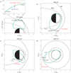 |
Fig. 1 MAVEN orbit information. (a) MAVEN trajectory (green line) for the time interval of orbit 822, on March 3, 2015, shown in cylindrical (CYL) MSO coordinates frame. The blue and red arrows mark the positions of MAVEN at the arrival times of the transmitted IP shock and discontinuity-like structure, respectively, (b–d) the same trajectory on the MSO XY, XZ, and YZ planes. The two dashed black curves in each panel represent the average locations of the BS and magnetic pileup boundary. |
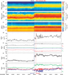 |
Fig. 2 Overview plots of the transmitted shock and discontinuity-like structure encountered by MAVEN. (a) On-board-computed ion energy spectra. (b) Ion energy spectra computed on the ground from the Coarse 3D data. (c) Electron energy spectra. (d) Proton density. (e) Proton velocity components in MSO coordinates and proton bulk speed. (f) Magnetic field magnitude. (g) Magnetic field components in MSO coordinates. The vertical dashed blue and red lines correspond to the transmitted IP shock and discontinuity-like structure, respectively. |
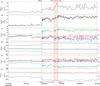 |
Fig. 3 Zoom-in plot of magnetic field and plasma parameters around the discontinuity-like structure. (a) Proton density. (b) Magnetic field magnitude. (c) Magnetic field components in MSO coordinates. (d) Proton velocity components in MSO coordinates and proton bulk speed. (e) Magnetic field components in local LMN coordinates. (f) Proton velocity components in local LMN coordinates. The upstream and downstream averages are shown as horizontal dashed red lines in the panels of ion density and magnetic field strength. The vertical dashed blue line indicates the transmitted IP shock. The shaded region bounded by vertical dashed red lines indicates the discontinuity-like structure interval. |
4 Generation mechanism of discontinuity
A question arises as to how the discontinuity-like structure generates. The interaction of the IP shock with the Martian BS comes to mind immediately as the most probable explanation for the discontinuity-like structure, because of the remarkable similarities between the phenomena observed on Earth and Mars. First, the presence of the discontinuity-like structure preceded by a fast transmitted IP shock is in agreement with the spacecraft observations at Earth and with predictions of the MHD theory, which demonstrate that a FF IP shock passing through the Earth’s BS would create a new discontinuity that follows the IP shock. The newly created discontinuity is a combination of several different kinds of discontinuities. As was suggested by Samsonov et al. (2006), they are composed of three discontinuities: a forward slow expansion wave, a contact discontinuity, and a reversed slow shock. These three discontinuities propagate with similar velocities (close to the local bulk flow velocity) in the magnetosheath, and thus they cannot be distinguished in the model or in spacecraft data. As a result, they could be identified as just one discontinuity. Second, the temporal separation between the shock and the discontinuity-like structure is on the order of tens of seconds, which matches reasonably well the scenario at Earth, where the transmitted shock propagates faster than the discontinuity and their temporal separation ranges from seconds to tens of seconds, depending on the location of the spacecraft in the magnetosheath. Third, the profiles of the magnetic field and plasma parameters across the discontinuity-like structure are quite consistent with those shown in the spacecraft observations at Earth and in the MHD simulations; for example, the magnetic field strength and ion density increase, and the velocity remains nearly unchanged (e.g., Samsonov et al. 2006; Zhang et al. 2012). Taken together, the MAVEN observations and related theoretical works indicate that the discontinuity-like structure is a compound structure in nature, composed of the slow expansion wave, contact discontinuity, and slow shock. This helps us understand why it cannot be classified as a particular discontinuity in MAVEN spacecraft data.
We further investigated the electron kinetic properties associated with the discontinuity-like structure. Figure 4 shows the omnidirectional differential particle flux and pitch angle (PA) distribution of suprathermal electrons (15–1000 eV) during the interval 18:16:00–18:21:00 UT, containing the discontinuity-like structure. We can see that the suprathermal electrons with different energies exhibit quite different PA distributions. More specifically, the 15–35 eV electrons show a relatively complex PA distribution, but it is clear that more of them distribute at small PAs (less than ~60°). The 39–55 eV electrons exhibit a bidirectional beam at both ~0° and ~180° PA. The 62–1000 eV electrons are nearly isotropic and are present at all PAs. It is interesting to note that, across the discontinuity, the high-energy suprathermal electrons (62–1000 eV) do not show any appreciable changes, whereas the lower-energy suprathermal electrons (15–35 eV and 39–55 eV) display remarkable enhancements in their fluxes. The electron flux enhancements serve as an additional discriminative feature for the discontinuity-like structure, and could be mainly attributed to the newly created contact discontinuity. According to previous theoretical studies, the variations in plasma parameters across the slow expansion wave and slow shock are smaller than those across the contact discontinuity (Grib 1982; Samsonov et al. 2006). They might have resulted in a relatively small decrease in the electron density, but it is masked by a stronger increase in the electron density across the contact discontinuity.
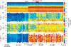 |
Fig. 4 Electron omnidirectional differential fluxes and electron PA distribution during the interval 18:16:00–18:21:00 UT. (a) Omnidirectional differential fluxes of the 3–4627 eV electrons. (b)–(d) PA distributions of suprathermal electrons in the energy range of 15–35 eV, 39–55 eV, and 62–1000 eV, respectively. The vertical dashed blue line indicates the transmitted IP shock. The two vertical dashed black lines mark the discontinuity-like structure interval. |
5 Conclusions
In this paper, we report the first observation of a discontinuity-like structure created by the interaction of a fast IP shock with the BS at Mars. The transmitted IP shock propagating through the magnetosheath was encountered by the MAVEN spacecraft at 18:17:53 UT on March 3, 2015. It is a quasi-perpendicular shock with shock angle of ~74.82 degrees and shock strength of ~2.45, and propagates toward Mars with a speed of ~544.59 km s−1. The discontinuity-like structure follows the transmitted IP shock, and their temporal separation is about 41 seconds. The discontinuity-like structure is characterized by an increase in magnetic field strength, remarkable enhancements in particle fluxes for both ions and lower-energy suprathermal electrons (15–35 eV and 39–55 eV), and no visible change in ion velocity. These distinctive features show good agreement with the predictions of the MHD theory and with the observations at Earth. The comparison of MAVEN measurements with theoretical studies indicates that the discontinuity-like structure is a compound structure in nature, composed of the slow expansion wave, contact discontinuity, and slow shock. This event adds new insights to our understanding of the interaction of a fast IP shock with the BS at unmagnetized planets. It will be necessary in future studies to investigate the propagation of the IP shock through the Martian magnetosheath and the interaction of the IP shock with the Martian magnetopause.
Acknowledgements
This work is supported by the Strategic Priority Research Program of Chinese Academy of Sciences, Grant No. XDB 41000000, the National Natural Science Foundation of China (NSFC) (42374214, 42074212, 42030202), the Key Research Program of the Institute of Geology and Geophysics, CAS, grant IGGCAS-201904, the pre-research Project on Civil Aerospace Technologies No. D020104 funded by Chinese National Space Administration. The MAVEN project is supported by NASA through the Mars Exploration Program. We have used the MAVEN plasma and magnetic field data throughout. The PDS Planetary Plasma Interactions Node (https://pds-ppi.igpp.ucla.edu/) makes the MAVEN data publically available. We appreciate the data being made available by the PIs of MAG (J.E.P. Connerney), SWIA (J.S. Halekas), and SWEA (D.L. Mitchell) on board MAVEN.
References
- Acuna, M. H., Connerney, J. E. P., Wasilewski, P., et al. 1998, Science, 279, 1676 [NASA ADS] [CrossRef] [Google Scholar]
- Acuna, M. H., Connerney, J. E. P., Ness, N. F., et al. 1999, Science, 284, 790 [NASA ADS] [CrossRef] [Google Scholar]
- Akhiezer, A. I. 1975, Plasma Electrodynamics - Vol.1: Linear Theory; Vol. Non-linear Theory and Fluctuations (Oxford: Pergamon Press) [Google Scholar]
- Barabash, S. 2012, Earth Planets Space, 64, 57 [NASA ADS] [CrossRef] [Google Scholar]
- Blanco-Cano, X., Omidi, N., & Russell, C. T. 2004, Astron. Geophys., 45, 3.14 [NASA ADS] [CrossRef] [Google Scholar]
- Brain, D. A., Halekas, J. S., Lillis, R., et al. 2005, Geophys. Res. Lett., 32, L18203 [Google Scholar]
- Connerney, J. E. P., Espley, J., Lawton, P., et al. 2015, Space Sci. Rev., 195, 257 [NASA ADS] [CrossRef] [Google Scholar]
- Dubinin, E., Lundin, R., Koskinen, H., & Norberg, O. 1993, J. Geophys. Res., 98, 5617 [NASA ADS] [CrossRef] [Google Scholar]
- Dubinin, E., Obod, D., Lundin, R., Schwingenschuh, K., & Grard, R. 1995, Adv. Space Res., 15, 423 [NASA ADS] [CrossRef] [Google Scholar]
- Ganushkina, N. Y., Liemohn, M. W., & Dubyagin, S. 2018, Rev. Geophys., 56, 309 [NASA ADS] [CrossRef] [Google Scholar]
- Grib, S. A. 1982, Space Sci. Rev., 32, 43 [NASA ADS] [CrossRef] [Google Scholar]
- Grib, S. A., Briunelli, B. E., Dryer, M., & Shen, W. W. 1979, J. Geophys. Res., 84, 5907 [NASA ADS] [CrossRef] [Google Scholar]
- Halekas, J. S., Taylor, E. R., Dalton, G., et al. 2015, Space Sci. Rev., 195, 125 [CrossRef] [Google Scholar]
- Halekas, J. S., Brain, D. A., Luhmann, J. G., et al. 2017a, J. Geophys. Res. Space Phys., 122, 11320 [NASA ADS] [Google Scholar]
- Halekas, J. S., Ruhunusiri, S., Harada, Y., et al. 2017b, J. Geophys. Res. Space Phys., 122, 547 [NASA ADS] [CrossRef] [Google Scholar]
- He, L., Guo, J., Zhang, F., et al. 2023, A&A, 679, A79 [NASA ADS] [CrossRef] [EDP Sciences] [Google Scholar]
- Huang, H., Guo, J., Wang, Z., et al. 2019, ApJ, 879, 118 [NASA ADS] [CrossRef] [Google Scholar]
- Huang, H., Guo, J., Mazelle, C., et al. 2021, ApJ, 914, 14 [NASA ADS] [CrossRef] [Google Scholar]
- Intriligator, D. S., & Smith, E. J. 1979, J. Geophys. Res., 84, 8427 [NASA ADS] [CrossRef] [Google Scholar]
- Jakosky, B. M., Grebowsky, J. M., Luhmann, J. G., et al. 2015a, Science, 350, 0210 [Google Scholar]
- Jakosky, B. M., Lin, R. P., Grebowsky, J. M., et al. 2015b, Space Sci. Rev., 195, 3 [CrossRef] [Google Scholar]
- Koval, A., Šafránková, J., Němeček,, Z., et al. 2005, Geophys. Res. Lett., 32, L15101 [CrossRef] [Google Scholar]
- Koval, A., Šafránková, J., Němeček, Z., & Přech, L. 2006, Adv. Space Res., 38, 552 [NASA ADS] [CrossRef] [Google Scholar]
- Mitchell, D. L., Mazelle, C., Sauvaud, J. A., et al. 2016, Space Sci. Rev., 200, 495 [NASA ADS] [CrossRef] [Google Scholar]
- Moses, S. L., Coroniti, F. V., & Scarf, F. L. 1988, Geophys. Res. Lett., 15, 429 [NASA ADS] [CrossRef] [Google Scholar]
- Pallocchia, G. 2013, J. Geophys. Res. Space Phys., 118, 331 [NASA ADS] [CrossRef] [Google Scholar]
- Pallocchia, G., Samsonov, A. A., Bavassano Cattaneo, M. B., et al. 2010, Annal. Geophys., 28, 1141 [NASA ADS] [CrossRef] [Google Scholar]
- Ramstad, R., Brain, D. A., Dong, Y., et al. 2020, Nat. Astron., 4, 979 [CrossRef] [Google Scholar]
- Russell, C. T., Wang, Y. L., Raeder, J., et al. 2000, J. Geophys. Res., 105, 25143 [CrossRef] [Google Scholar]
- Šafránková, J., Němeček, Z., Přech, L., et al. 2007, J. Geophys. Res. Space Phys., 112, A08212 [Google Scholar]
- Samsonov, A. A. 2011, J. Atmos. Sol.-Terres. Phys., 73, 30 [NASA ADS] [CrossRef] [Google Scholar]
- Samsonov, A. A., Němeček, Z., & Šafránková, J. 2006, J. Geophys. Res. Space Phys., 111, A08210 [NASA ADS] [CrossRef] [Google Scholar]
- Sonnerup, B. Ö., & Cahill Jr, L. 1967, J. Geophys. Res., 72, 171 [Google Scholar]
- Thampi, S. V., Krishnaprasad, C., Bhardwaj, A., et al. 2018, J. Geophys. Res. Space Phys., 123, 6917 [NASA ADS] [CrossRef] [Google Scholar]
- Yan, M., & Lee, L. C. 1996, J. Geophys. Res., 101, 4835 [NASA ADS] [CrossRef] [Google Scholar]
- Zhang, H., Sibeck, D. G., Zong, Q. G., et al. 2012, Annal. Geophys., 30, 379 [NASA ADS] [CrossRef] [Google Scholar]
- Zhuang, H. C., Russell, C. T., Smith, E. J., & Gosling, J. T. 1981, J. Geophys. Res., 86, 5590 [NASA ADS] [CrossRef] [Google Scholar]
All Figures
|
Fig. 1 MAVEN orbit information. (a) MAVEN trajectory (green line) for the time interval of orbit 822, on March 3, 2015, shown in cylindrical (CYL) MSO coordinates frame. The blue and red arrows mark the positions of MAVEN at the arrival times of the transmitted IP shock and discontinuity-like structure, respectively, (b–d) the same trajectory on the MSO XY, XZ, and YZ planes. The two dashed black curves in each panel represent the average locations of the BS and magnetic pileup boundary. |
| In the text | |
|
Fig. 2 Overview plots of the transmitted shock and discontinuity-like structure encountered by MAVEN. (a) On-board-computed ion energy spectra. (b) Ion energy spectra computed on the ground from the Coarse 3D data. (c) Electron energy spectra. (d) Proton density. (e) Proton velocity components in MSO coordinates and proton bulk speed. (f) Magnetic field magnitude. (g) Magnetic field components in MSO coordinates. The vertical dashed blue and red lines correspond to the transmitted IP shock and discontinuity-like structure, respectively. |
| In the text | |
|
Fig. 3 Zoom-in plot of magnetic field and plasma parameters around the discontinuity-like structure. (a) Proton density. (b) Magnetic field magnitude. (c) Magnetic field components in MSO coordinates. (d) Proton velocity components in MSO coordinates and proton bulk speed. (e) Magnetic field components in local LMN coordinates. (f) Proton velocity components in local LMN coordinates. The upstream and downstream averages are shown as horizontal dashed red lines in the panels of ion density and magnetic field strength. The vertical dashed blue line indicates the transmitted IP shock. The shaded region bounded by vertical dashed red lines indicates the discontinuity-like structure interval. |
| In the text | |
|
Fig. 4 Electron omnidirectional differential fluxes and electron PA distribution during the interval 18:16:00–18:21:00 UT. (a) Omnidirectional differential fluxes of the 3–4627 eV electrons. (b)–(d) PA distributions of suprathermal electrons in the energy range of 15–35 eV, 39–55 eV, and 62–1000 eV, respectively. The vertical dashed blue line indicates the transmitted IP shock. The two vertical dashed black lines mark the discontinuity-like structure interval. |
| In the text | |
Current usage metrics show cumulative count of Article Views (full-text article views including HTML views, PDF and ePub downloads, according to the available data) and Abstracts Views on Vision4Press platform.
Data correspond to usage on the plateform after 2015. The current usage metrics is available 48-96 hours after online publication and is updated daily on week days.
Initial download of the metrics may take a while.