| Issue |
A&A
Volume 673, May 2023
|
|
|---|---|---|
| Article Number | A3 | |
| Number of page(s) | 6 | |
| Section | Planets and planetary systems | |
| DOI | https://doi.org/10.1051/0004-6361/202244139 | |
| Published online | 26 April 2023 | |
Effects of the Parker spiral angle of the interplanetary magnetic field on the dawn-dusk asymmetry of the Martian magnetotail
1
School of Space and Environment, Beihang University,
Beijing
100191,
PR China
2
Key Laboratory of Space Environment Monitoring and Information Processing, Ministry of Industry and Information Technology,
Beijing
100191,
PR China
e-mail: This email address is being protected from spambots. You need JavaScript enabled to view it.
Received:
29
May
2022
Accepted:
2
February
2023
Abstract
Context. The draping of the interplanetary magnetic field (IMF) around unmagnetized planets induces a magnetotail with a two-lobe plasma structure. On Mars, due to the impact of the IMF Parker spiral angle, the structure of its induced magnetotail is dawn-dusk asymmetric. Observational and numerical studies have shown the dawn-dusk asymmetric size of magnetic lobes and the shift of the polarity reversal layer and the inverse polarity reversal layer under different Parker spiral angles. Variation in the tail-region induced magnetic field with the Parker spiral angle is important in the evolution of the magnetotail. Further studies should investigate the influence of the magnetic pressure and field direction on the magnetic lobe structure and plasma boundary locations, as well as the relationship between the polarity reverse of the IMF and the Parker spiral angle.
Aims. This study aims to investigate the dawn-dusk asymmetric structure of the Martian magnetotail under different Parker-spiral IMF orientations. In this study, we used a multispecies magnetohydro-dynamic (MHD) model, which has been shown to self-consistently calculate the Mars-solar wind interaction, to investigate the effects of the Parker spiral angle on the structure of the Martian magnetotail. By comparing the magnetic field, large-scale configurations, and plasma boundary locations across various cases, we aim to clarify how variations in the IMF Parker spiral angle affect the magnetic pressure and field direction in the magnetotail and the locations and shapes of the magnetic lobes, polarity reversal layer, and inverse polarity reversal layer.
Methods. A three-dimensional and parallelized multispecies MHD model was constructed to simulate the global solar wind interaction with Mars. Four ion species, H+, O2+, O+, and CO2+, as well as the chemical reactions between them, such as photoionization, charge exchange, and recombination, were considered in the model to accurately calculate the ion distributions in the magnetosphere and ionosphere of Mars. Three cases with Parker spiral angles of 90, 56, and 30 degrees were examined, representing the perpendicular, standard, and quasi-parallel IMF relative to the solar wind flow, respectively.
Results. A symmetric magnetotail was reproduced in the case with a Parker spiral angle of 90° degrees. When the Parker spiral angle decreases, the magnetic pressure in the magnetic lobes reduces, and the flaring angle of the magnetic field becomes larger on the dawn side than on the dusk side. These two factors result in the shrinkage and extension of the magnetic lobes. Furthermore, the variation in magnetic pressure results in a polarity reversal layer bent toward the dawn side. Finally, we found that the inverse polarity reversal layer shrinks toward Mars with a decrease in the Parker spiral angle.
Key words: magnetohydrodynamics (MHD) / methods: numerical / planets and satellites: magnetic fields
© The Authors 2023
 Open Access article, published by EDP Sciences, under the terms of the Creative Commons Attribution License (https://creativecommons.org/licenses/by/4.0), which permits unrestricted use, distribution, and reproduction in any medium, provided the original work is properly cited.
This article is published in open access under the Subscribe to Open model. This email address is being protected from spambots. You need JavaScript enabled to view it. to support open access publication.
1 Introduction
The magnetic environment of Mars is different from that of Earth because solar wind interacts directly with the Martian ionosphere and upper atmosphere in the absence of an intrinsic magnetic field. This interaction forms the magnetosheath, magnetic pileup region (MPR), magnetotail, and other large-scale configurations (Nagy et al. 2004). As a result of an interplanetary magnetic field (IMF) pileup, the induced magnetotail on the nightside of Mars is composed of two magnetic lobes with opposite field directions (Crider et al. 2004; Brain et al. 2007), and between these magentic lobes there is a cross-tail current sheet with a small-magnitude magnetic field (Brain 2006; Xu et al. 2016; Liemohn et al. 2018). Recently, observational analysis from the Mars Atmosphere and Volatile Evolution mission has indicated that the Martian crustal fields and the variable IMF influence the structure of the magnetotail, resulting in a steady and kink-like flapping of the current sheet (e.g., DiBraccio et al. 2017), twisting of the total magnetotail structure (e.g., DiBraccio et al. 2018), and the formation of small local current sheets (e.g., Grigorenko et al. 2017).
The influence of the IMF orientation on the magnetotail structure of unmagnetized planets and moons, such as Mars, Venus, and Titan, is an important subject (McComas et al. 1986; Brain et al. 2007; Bertucci et al. 2011; Romanelli et al. 2014, 2015). Although the Martian crustal fields, which are primarily distributed on the southern hemisphere (Acuna et al. 1999), exert a twisting effect on the magnetotail structure, the formation and variation of the large-scale configuration of the Martian magnetotail are mainly controlled by the solar wind upstream and IMF conditions (Li et al. 2021; Liemohn et al. 2017; Romanelli et al. 2014). Due to the impact of the IMF Parker spiral angle, the location of the induced magnetotail relative to the planet is dawn-dusk asymmetric (Li et al. 2021; Romanelli et al. 2015). Meanwhile, the sizes of the two magnetic lobes, as well as the twisting and shifting directions of the current sheet in the magnetotail, are also influenced by the solar wind upstream conditions (Harnett et al. 2005; Halekas et al. 2006; Xu et al. 2016; Liemohn et al. 2017). McComas et al. (1986) provided an explanation of how the Parker spiral IMF causes the asymmetric dawn-dusk distribution of the magnetic flux and magnetic pressure in the Venusian magnetotail and consequently results in an asymmetric magnetotail structure. This effect has been confirmed by global magnetohydro-dynamic (MHD) simulations of the solar wind interaction with Venus (Ma et al. 2013).
Previous numerical studies have described the structure of the Martian magnetotail at a Parker spiral angle of 56° (Ma et al. 2002, 2004; Najib et al. 2011; Xu et al. 2016; Liemohn et al. 2017; Li et al. 2020). Although the average value of the Parker spiral angle is close to 30°–60° near Venus and Mars, statistical analysis has indicated that quasi-parallel (0°–30°) and quasi-vertical (80°–90°) IMFs occur with a high frequency (Chang et al. 2018; Liu et al. 2021). In the case of quasi-vertical IMF, the magnetic field around an unmagnetized planet has a more regular shape, for example, the magnetotail structure of the planet will be approximately dawn-dusk symmetric (Romanelli et al. 2014; DiBraccio et al. 2018; Li et al. 2021). However, a more complex configuration of the magnetic field appears when IMF is quasi-parallel, which makes the near planetary environment more coupled with the solar wind to effectively transfer the solar wind energy to ionospheric ions (Masunaga et al. 2011). Additionally, plasma boundaries such as the bow shock (BS) and magnetic pileup boundary (MPB) shrink toward Mars (Chang et al. 2018; Li et al. 2021). Observational results have indicated that the IMF is located on the ecliptic plane in most cases, with an average magnitude of 3.3 nT (DiBraccio et al. 2018), and the Parker spiral angle presents a bimodal distribution between −180° and 180° with two peak values (Liu et al. 2021). Nevertheless, the effect of the Parker spiral angle on the structure of the Martian magnetotail remains unclear.
In this study, we aim to explore the influence of the Parker spiral angle of the IMF on the shaping of the structure and dawn-dusk asymmetry of the Martian magnetotail using a multispecies MHD numerical model, which can self-consistently calculate the plasma and magnetic environment around Mars. We performed the numerical simulations with typical IMF Parker spiral angles to demonstrate the responses of the magnetotail structure to the changes in IMF orientation and removed the crustal fields to avoid their influence. Moreover, we present the size and location of the magnetic lobes, the average direction of the induced magnetotail, and the magnetic pressure under different IMF orientations.
2 Model description
We employed a three-dimensional multispecies MHD model to simulate the Mars-solar wind interaction, which includes a set of four continuity equations for the ion species H+,  , O+, and
  , with a high contribution in the Martian ionosphere. A set of eight wave MHD equations was used in the model and augmented with a series of ionospheric chemical reactions, including photoionization, charge exchange, and dissociative recombination. The primary theory of the model is based on that proposed by Ma et al. (2004), which integrates the MHD equations with the mass conservation equation for individual ion species. In our model, the mass equations with respect to the four ion species were decoupled with the main MHD equations, shown below, to facilitate the implementation of the calculation method (Li et al. 2021):
![Mathematical equation: ${\partial \over {\partial t}}\left[ {\matrix{ {{\rho _1}} \cr {{\rho _2}} \cr {{\rho _3}} \cr {{\rho _4}} \cr } } \right] + \nabla \cdot \left[ {\matrix{ {{\rho _1}{\bf{u}}} \cr {{\rho _2}{\bf{u}}} \cr {{\rho _3}{\bf{u}}} \cr {{\rho _4}{\bf{u}}} \cr } } \right] = \left[ {\matrix{ {{S_1} - {L_1}} \cr {{S_2} - {L_2}} \cr {{S_3} - {L_3}} \cr {{S_4} - {L_4}} \cr } } \right].$](/articles/aa/full_html/2023/05/aa44139-22/aa44139-22-eq5.png) (1)
(1)
Here, mass production and loss rate are represented by Si and Li, respectively, for i ion species.
The decoupled MHD equations refer to the model of Li et al. (2021), which has been shown to suitably describe the plasma environment in the Mars-solar wind interaction without the crustal fields. In this study, our model was parallelized to improve computing speed. Moreover, the photoionization effect was included in the model by adopting the Chapman function, which has been shown to significantly improve the agreement with plasma density observations (Ma et al. 2015). Thus, our model can accurately calculate the distribution of the magnetic field and plasma in the dayside ionosphere. The MHD equations can be expressed as follows:
![Mathematical equation: $\matrix{ {{\partial \over {\partial t}}\left[ {\matrix{ {\sum _{i = 1}^4{\rho _i}} \cr {\left( {\sum _{i = 1}^4{\rho _i}} \right){\bf{u}}} \cr {\bf{B}} \cr \varepsilon \cr } } \right] + \nabla \cdot \left[ {\matrix{ {\sum _{i = 1}^4{\rho _i}{\bf{u}}} \cr {\left( {\sum _{i = 1}^4{\rho _i}} \right){\bf{uu}} + \left( {p + {{{B^2}} \over 2}} \right){\bf{I}} - {\bf{BB}}} \cr {{\bf{uB}} - {\bf{Bu}}} \cr {{\bf{u}}\left( {\varepsilon + p + {{{B^2}} \over 2}} \right) - \left( {{\bf{B}} \cdot {\bf{u}}} \right){\bf{B}}} \cr } } \right]} \cr {\,\,\,\,\,\,\, = \left[ {\matrix{ {\sum _{i = 1}^4{S_i} - \sum _{i = 1}^4{L_i}} \cr {\left( {\sum _{i = 1}^4{\rho _i}} \right){\bf{g}} - \left( {\sum _{i = 1}^4{\rho _i}} \right)v{\bf{u}} - \left( {\sum _{i = 1}^4{L_i}} \right){\bf{u}}} \cr 0 \cr {{Q_E}} \cr } } \right]\,\,\,\,\,\,\,\,\,\,\,\,\,\,\,\,\,\,\,\,\,\,\,\,\,\,\,\,\,\,} \cr } ,$](/articles/aa/full_html/2023/05/aa44139-22/aa44139-22-eq6.png) (2)
(2)
where, Qe in Eq. (2) is defined as:
 (3)
(3)
where, TE in Eq. (3) is defined as follows (Ma et al. 2004):
![Mathematical equation: ${T_E} = 4 \times {10^{ - 11}}\sum\limits_{t = 1}^3 {{n_t}} \sum\limits_{i = 1}^4 {{{{\rho _i}} \over {{m_i}}}\exp \left[ {{{10\left( {{T_p} - 6000} \right)} \over {{T_p}}}} \right].}$](/articles/aa/full_html/2023/05/aa44139-22/aa44139-22-eq8.png) (4)
(4)
In Eq. (2), ρ1, ρ2, ρ3, and ρ4 are the mass densities of H+,  , O+, and
  , respectively, and и is the plasma velocity. The total energy density ε is defined as
  ; p is the total thermal pressure of the plasma; ν is the ion neutral collision frequency; T0 is the temperature of the newly produced ions, which is assumed to be the same as the temperature of the local neutral atmosphere; γ is the ratio of specific heats (considered as 5/3); n1, n2, and n3 are the number densities of the neutral component CO2, O, and H, respectively; and Tp is the plasma temperature calculated as
  under the assumption of equal temperature between ions and electrons. The other symbols in the above equations retain their usual definitions. The source term QE, Eq. (3), was added in the energy conservation equation of our MHD model in order to consider the inelastic collisions between different species and to include chemical reactions such as photoionization, charge exchange, and recombination. The specific chemical reactions and reaction rates were obtained from previous studies (Ma et al. 2004; Schunk et al. 2009).
Our calculations were performed in the Mars Solar Orbital coordinate system with the x-axis pointing from Mars toward the Sun, the z-axis perpendicular to the x-axis and positive toward the north celestial pole, and the y-axis completing the right side coordinate system. The simulation domain is within −24 RM ≤ X ≤ 8RM and −16M ≤ Y, Z ≤ 16 Rm, where RM is the radius of Mars (3396 km). The calculation grid was generated in a generalized curvilinear coordinate, which facilitated grid clustering in regions with substantial physical variation. The inner boundary of the grid was set as 100 km above the Martian surface, and for the densities of the ions  , O+, and
  , photochemical equilibrium values were considered. The normal velocity value at the boundary was set to zero based on the assumption of an inviscid fluid. The setups of the neutral atmospheric components and solar wind refer to those in Li et al. (2021). Lastly, the density of H+ is 30% of the solar wind density (Taylor et al. 1980).
To study the influence of the IMF with different Parker spiral angles on the structure of the magnetotail, three cases with Parker spiral angles of 90°, 56°, and 30° were examined. In this study, the Parker spiral angle is defined as the acute angle between the IMF and x-axis. The IMF parameter settings for the three cases are listed in Table 1. A Parker spiral angle of 90° indicates that the Bx component of the IMF is zero, and a parker spiral angle of 30° represents the case when the IMF is quasiparallel to the solar wind flow. The IMF is in the X–Y plane with a fixed value of 3 nT and has a positive BY component.
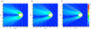 |
Fig. 1 Distribution of the induced magnetic field strength in the X–Y plane for different Parker spiral angles. Panel a: 90°; panel b: 56°; panel c: 30°. White solid lines represent magnetic field lines. |
IMF parameter settings of the computational cases.
3 Numerical results
Figure 1 shows the distribution of the induced magnetic field strength (|B|) in the X–Y plane for cases with Parker spiral angles of 90, 56, and 30°. The magnetic field lines are superimposed on the figures to show the general characteristics of the Martian plasma environment (Nagy et al. 2004; Ma et al. 2004; Najib et al. 2011). The traces and distributions of the magnetic field lines agree well with the schematic presented by McComas et al. (1986). On the dayside, an obvious boundary layer exhibiting a jump in magnetic field strength from the weaker background magnetic field (approximately 3 nT) to over 10 nT represents the location of the BS in all cases. Inside the BS, the red regions where the magnetic field strength is enhanced represents the MPR, in which the magnetic field lines are highly piled up. As the Parker spiral angle changes from 90° to 30°, the peak strength of the induced magnetic field in the MPR decreases from 55 nT to 40 nT. On the nightside, the induced magnetotail with a plasma structure composed of two lobes forms because of the draping of the magnetic field lines. The symmetrical structure of the magnetotail shown in Fig. 1a is evidently different from that in Figs. 1b and c, in which the entire configuration of the magnetotail moves toward the dawn side.
To quantitatively describe the dawn-dusk asymmetry in this study, the pressure balance boundary, defined as the position where the magnetic pressure Pb and the thermal pressure Pt are balanced, was used (Xu et al. 2016). Figure 2 presents the distribution of the logarithmic pressure ratio β = log10 (Pt/Рb) in the X–Y plane for cases with Parker spiral angles of 90, 56, and 30. The iso-gram of β = 0 is the location of the pressure balance boundary. On the nightside, the region defined by the black lines represent the magnetic lobes of the magnetotail where the magnetic pressure Pb dominates. The dawn-dusk asymmetry of the Martian magnetotail can be determined by the difference in the sizes of the magnetic lobes. As shown in Fig. 2a, the size of the magnetic lobes on both sides was approximately the same. As the Parker spiral angle decreased from 90° (Fig. 2a) to 56° (Fig. 2b), the length of the dawn-side lobe shrank from 7 RM to 4 RM, whereas the length of the dusk-side lobe expanded from 9 RM to over 10.5 RM, and its width expanded by 1.5 times within the given range. Figure 2c shows that the length of the magnetic lobe shrank from 4 RM (Fig. 2b) to 3 RM (Fig. 2c) on the dawn side and from over 10.5 RM (Fig. 2b) to 7 RM (Fig. 2c) on the dusk side. Furthermore, in order to demonstrate the complete size of the magnetic lobes, the three-dimensional pressure balance boundary represented by the iso-surface of β = 0 is shown in Fig. 3. In the Z direction, the width of the magnetic lobes is between 1.2 RM and 1.4 RM. Figures 2 and 3 show that the overall configuration of the magnetotail is symmetrical when the Parker spiral angle is 90°. However, the dusk side lobe tends to be larger than the dawn side lobe when the Parker spiral angle is not 90°. In addition, Figs. 2c and 3 show that the two magnetic lobes shrink when the IMF is quasi-parallel to the solar wind flow.
The polarity reversal layer (PRL) is an important boundary produced in the interaction region between a magnetized plasma flow (solar wind) and a conducting obstacle (Mars, Venus, or Titan; Simon et al. 2013). It can be represented by the position where the flow-aligned component of magnetic field reverses its polarity. In addition, Romanelli et al. (2014) identify a layer called the inverse polarity reversal layer (IPRL) in the downstream region far from the central magnetotail. The change in the sign of the flow-aligned component of the IPRL is opposite to that of the PRL. The locations of the PRL and IPRL respond to the change of the IMF orientation, and thus they can be used to characterize the location and size of the draped magnetotail configurations in different cases (Romanelli et al. 2014, 2015).
In this model, based on the direction of the solar wind (along x-axis), the PRL and IPRL can be characterized by an iso-gram of BX = 0. The positions of the PRL and IPRL are presented in Fig. 4 and demonstrate the distribution of BX components of the induced magnetic field in the X–Y plane. In Fig. 4a, it is evident that the field lines mirror the x-axis when the Parker spiral angle is 90°, and the BX component reverses its polarity at Y = 0. Since the IMF is perpendicular to the x-axis, no IPRL exists in this case. In Figs. 4b, c, under the asymmetrical distribution of the magnetic field strength in the dawn side and dusk side magnetic lobes, the PRL shifts to the dawn side. The IPRL is located on the outside of the dawn side lobe, and the distance from the PRL to the IPRL gradually increases in the downstream. As the Parker spiral angle decreased from 56° (Fig. 4b) to 30° (Fig. 4c), the IPRL shrank toward Mars.
Figure 5 shows the iso-gram of BX = 0 in the Y–Z plane at X = −2 RM and −4 RM for cases with different Parker spiral angles. In the case where the Parker spiral angle is 90° degrees, the PRL is almost parallel to the Z-axis and can be regarded as the axis of symmetry for the two magnetic lobes. When the Parker spiral angle is not 90°, the shape of the iso-gram of BX = 0 is similar to a semi-ellipse in the Y–Z plane. In previous studies, researchers identified the part in the left (right) dashed box of the iso-grams as the IPRL (PRL; Simon et al. 2013; Romanelli et al. 2014). As the Parker spiral angle decreased, the central part of the iso-gram (red and blue lines, PRL) bent significantly to the dawn side, and the IPRL emerged on the dawn side and shrank toward Mars. In the −4 RM downstream case, the responses in the locations and structures of the PRL and IPRL to the change of the Parker spiral angle are more obvious than in the −2 RM downstream case. Based on Figs. 4 and 5, it can be concluded that the iso-surface of BX = 0 in 3D space is similar to an elliptical cylinder with an expanding cross-section in the anti-Mars direction. This result indicates that the presence of Mars in the magnetized solar wind flow has an insufficient influence on the IMF to reverse the polarity of the BX component outside the region surrounded by the iso-surface of BX = 0.
Figure 6 presents the variation in the magnetic pressure with Y at Z = 0 RM at X = −2 RM and at X = −4 RM downstream. All the curves in the figure have two peaks, which can be regarded as the regions of magnetic lobes, and a trough between the two magnetic lobes. As the Parker spiral angle decreased, the troughs of the curves moved to Y = −0.4 RM (Fig. 6a) and Y = −0.8 RM (Fig. 6b). In the −2 RM downstream case (Fig. 6a), the peaks of magnetic pressure on both sides decreased from 0.17 nPa to 0.13 nPa, responding to the Parker spiral angle change from 90° to 30°. In the −4 RM downstream case (Fig. 6a), the decrease in the magnetic pressure on the dawn side (from 0.13 nPa to 0.06 nPa) is twice the decrease on the dusk side (from 0.13 nPa to 0.095 nPa), indicating that when the Parker spiral angle decreases, the dawn-side magnetic lobe is affected to a greater degree compared to the dusk-side lobe.
The flaring of the magnetic field lines in the magnetotail is also an important diagnostic parameter in the dawn-dusk asymmetry of the magnetotail. The flaring angle θf = arceos (BX/|B|) is a characterization of the magnetic field direction and is related to the magnetotail width and the shape alteration of the plasma boundaries in the magnetotail (Crider et al. 2004). In this study, the acute angle between the induced magnetic field and the x-axis is calculated to specifically represent the flaring angle in the Martian magnetotail. Figure 7 shows the variation in the flaring angle at X = −4 RM for three cases. The flaring angle close to 0° (90°) indicates that the direction of the induced magnetic field is quasi-parallel (quasi-perpendicular) to the x-axis and the solar wind flow in this model. For all the cases in the figure, the flaring angle peaks near the central tail region (Y = 0 RM) represent the polarity reversion of the BX component, and the two troughs on both the dawn side and the dusk side correspond to the positions of the magnetic lobes. At Y = −4.8 RM in the 30° Parker spiral angle case and Y = −6 RM in the 56° Parker spiral angle case, the extra peaks represent the location of the IPRL. In the region of −3 RM ≤ Y ≤ 3 RM, the flaring angles in the 30° and 56° Parker spiral angle cases are higher than the flaring angle in the 90° Parker spiral angle case on the dawn side and lower than it on the dusk side. This result indicates that when the Parker spiral angle decreases, the average direction of the induced magnetotail on the dawn side (dusk side) becomes more perpendicular (parallel) to the solar wind flow compared to the case for a Parker spiral angle of 90°.
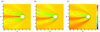 |
Fig. 2 Distribution of the logarithmic pressure ratio β in the X–Y plane for different Parker spiral angles. Panel a: 90°; panel b: 56°; panel c: 30°. Black lines with ‘0’ labels represent the iso-gram of β = 0. |
 |
Fig. 3 Iso-surface of β = 0 in the 3D space for different Parker spiral angles. Left: (a) 90°; middle: (b) 56°; right (c): 30°. |
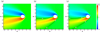 |
Fig. 4 Bx component of the induced magnetic field for different IMF directions with the Parker spiral angles of 90° (a), 56° (b), and 30° (c), respectively, in the X–Y plane. The red and blue areas represent the magnetic lobes with positive and negative BX components. Black lines with ‘0’ labels represent the iso-gram of Bx = 0. |
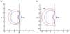 |
Fig. 5 Iso-gram of Bx = 0 in the Y–Z plane at X = −2 RM (a) and −4 RM (b). Different line colors represent different settings of the Parker spiral angle: 90° (black), 56° (red), and 30° (blue). |
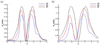 |
Fig. 6 Variation in the magnetic pressure with Y at Z = 0 RM in different cases of Parker spiral angles. Black: 90°; red: 56°; and blue: 30°. Left: (a) X = −2 RM; right: (b) X = −4 RM. |
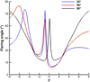 |
Fig. 7 Variation in the flaring angle on the line at X = −4 RM and Z = 0 RM in the Y–Z plane in different cases of Parker spiral angles. Black: 90°;red: 56°; and blue: 30°. |
4 Conclusions
In the present study, we investigated the effect of the Parker spiral angle on the dawn-dusk asymmetry of the Martian magnetotail by performing numerical simulations based on a three-dimensional multispecies MHD model. We conducted three numerical cases for Parker spiral angles of 90°, 56°, and 30°. The numerical results reproduced the distribution and draped structure of the induced magnetic field and indicated that a change in the value of the Parker spiral angle results in a change of the magnetic pressure and magnetic field direction in the Martian magnetotail, leading to the dawn-dusk asymmetrical structure of the magnetotail. Our conclusions about the varaition in the mangetic lobes and plasma boundaries under different IMF Parker spiral angles are as follows:
Previous numerical studies have indicated that without the crustal fields, the structure of the magnetotail is approximately symmetrical when the Parker spiral angle is 90° (Romanelli et al. 2014; Li et al. 2021). However, when the Parker spiral angle decreases, the dawn-side magnetic lobe shrinks significantly and becomes smaller than the dusk-side lobe. The size of the dawn-side magnetic lobe may be determined by two factors. First, the magnetic pressure in the magnetic lobes reduces with a decrease in the Parker spiral angle. In the distant magnetotail, the decrease in the magnetic pressure on the dawn side is twice the decrease on the dusk side, limiting the downstream extension of the dawn-side lobe. Second, the average direction of the induced magnetotail on the dusk side is more parallel to the solar wind flow than that on the dawn side. These two factors may be apt to maintain the magnetic pressure in the downstream and facilitate the extension of the magnetic lobes. Consequently, the dusk-side lobe becomes larger when the Parker spiral angle is 56°. When the Parker spiral angle is very small (i.e., when the IMF is quasi-parallel to the solar wind flow) due to a decrease in the magnetic pressure, the magnetic lobes on both the dusk and dawn sides shrink significantly;
The location of the PRL and IPRL can characterize the twist and dawn-dusk shift of the magnetotail. When the Parker spiral angle is not 90°, the PRL bends toward the dawn side due to the asymmetrical distribution of the magnetic pressure, especially near the equatorial plane of Mars. Moreover, the decrease in the Parker spiral angle leads to a decrease in the cross-flow IMF component (BY) and an increase in the flow-aligned IMF component (BX). This effect changes the direction of the induced magnetic field in the magnetic lobe and results in the formation and movement of the IPRL on the dawn side of Mars. When the IMF orientation changes, the shift of the IPRL is more obvious than that of the PRL. In fact, the region bounded by the PRL and IPRL can be regarded as the area in which the dawn-side IMF is strongly affected by the presence of Mars in the magnetized solar wind flow. As the Parker spiral angle decreases, this region shrinks toward Mars.
The draping pattern of the IMF around an unmagnetized planet and the resulting structure of the magnetotail are still worthy of further investigation. However, the existence of the crustal fields is why the Martian magnetotail is different from other unmagnetized planets. In the presence of the crustal fields, the variation in the IMF orientation can not only result in the dawn-dusk asymmetry of magnetic pressure on the magnetotail but also change the location of the reconnection between the IMF and the crustal fields (Weber et al. 2020). These effects periodically introduce open and closed magnetic topologies into the magnetotail and result in the clockwise or counterclockwise twist of the magnetotail structure from the ecliptic plane (DiBraccio et al. 2018, 2022; Ulusen et al. 2016). In this study, to ensure that the change occurring on the magnetotail is only caused by the change of the Parker spiral angle, the crustal fields were removed in the model. Furthermore, although the observational upstream solar wind and IMF conditions are variable, this study chose three typical cases to investigate the difference in the Martian magnetotail under different steady-state conditions. The results indicate the important effects of the IMF orientation on the configuration of the magnetotail, such as the systematic shift of the center-tail current sheet, variation in the magnetic pressure, and the difference in the size of the two magnetic lobes. Due to the similarities between the magnetotail structures of Mars and Venus (Dubinin et al. 2015), these conclusions may also be used as a reference for related research on the magnetotail structure of Venus.
Recent studies have indicated that the IMF orientation plays an important role in the transport processes of mass, energy, and momentum and that it controls the formation of the induced magnetosphere (Masunaga et al. 2011; Chang et al. 2020; Xu et al. 2021; Li et al. 2021). These physical processes are highly associated with planetary ion transport and the evolution of the Martian magnetotail. Thus, these subjects need to be further studied through numerical models.
Acknowledgements
This work was supported by the B-type Strategic Priority Program of the Chinese Academy of Sciences (Grant No. XDB41000000), and the National Natural Science Foundation of China (NSFC) under grant no. 42241114, 42074214 and 12150008, and the pre-research projects on Civil Aerospace Technologies nos. D020103 and D020105 funded by China’s National Space Administration (CNSA).
References
- Acuña M. H., Connerney, J. E. P., Ness, N. F., et al. 1999, Science, 284, 790 [NASA ADS] [CrossRef] [Google Scholar]
- Bertucci, C., Duru, F., Edberg, N., et al. 2011, SSR, 162, 113 [NASA ADS] [Google Scholar]
- Brain, D. A. 2006, SSR, 126, 77 [NASA ADS] [Google Scholar]
- Brain, D. A., Lillis, R. J., Mitchell, D. L., et al. 2007, JGRSP, 112, A09201 [Google Scholar]
- Chang, Q., Xu, X., Zhang, T., et al. 2018, ApJ, 867, 129 [Google Scholar]
- Chang, Q., Xu, X., Xu, Q., et al. 2020, ApJ, 900, 63 [Google Scholar]
- Crider, D. H., Brain, D. A., Acuna, M. H., et al. 2004, SSR, 111, 203 [NASA ADS] [Google Scholar]
- DiBraccio, G. A., Espley, J. R., Gruesbeck, J. R., et al. 2017, JGRSP, 122, 4308 [Google Scholar]
- DiBraccio, G. A., Luhmann, J. G., Curry, S. M., et al. 2018, GRL, 45, 4559 [NASA ADS] [CrossRef] [Google Scholar]
- DiBraccio, G. A., Romanelli, N., Bowers, C. F., et al. 2022, GRL, 49, e98007 [NASA ADS] [CrossRef] [Google Scholar]
- Dubinin, E., & Fraenz, M., 2015, Magnetotails of Mars and Venus (Wiley) [Google Scholar]
- Grigorenko, E. E., Shuvalov, S. D., Malova, H. V., et al. 2017, JGRSP, 122, 10176 [Google Scholar]
- Halekas, J. S., Brain, D. A., Lillis, R. J., et al. 2006, GRL, 22, 2449 [Google Scholar]
- Harnett, E. M., & Winglee, R. M., 2005, JGRSP, 110 [Google Scholar]
- Li, S. B., Lu, H. Y., Cui, J., et al. 2020, EPP, 4, 23 [Google Scholar]
- Li, Y., Lu, H., Cao, J., et al. 2021, ApJ, 921, 139 [NASA ADS] [CrossRef] [Google Scholar]
- Liemohn, M. W., & Xu, S. 2018, Recent Advances Regarding the Mars Magnetotail Current Sheet (Wiley) [Google Scholar]
- Liemohn, M. W., Xu, S., Dong, C., et al. 2017, JGRSP, 122 [Google Scholar]
- Liu, D., Rong, Z. J., Gao, J. W., et al. 2021, ApJ, 911, 113 [NASA ADS] [CrossRef] [Google Scholar]
- Ma, Y. J., Nagy, A. F., Kenneth, C., et al. 2002, JGR, 107, 1282 [NASA ADS] [CrossRef] [Google Scholar]
- Ma, Y. J., Nagy, A. F., Sokolov, I.V., et al. 2004, JGRSP, 109, A07211 [Google Scholar]
- Ma, Y. J., Nagy, A. F., Russell, C. T., et al. 2013, JGR, 118, 321 [NASA ADS] [Google Scholar]
- Ma, Y. J., Russell, C. T., Fang, X., et al. 2015, GRL, 42, 9113 [NASA ADS] [CrossRef] [Google Scholar]
- Masunaga, K., Futaana, Y., Yamauchi, M., et al. 2011, JGRSP, 116, A09326 [Google Scholar]
- McComas, D. J., Spence, H. E., Russell, C. T., et al. 1986, JGR, 91, 7939 [NASA ADS] [CrossRef] [Google Scholar]
- Nagy, A. F., Winterhalter, D., Sauer, K., et al. 2004, SSR, 111, 33 [NASA ADS] [Google Scholar]
- Najib, D., Nagy, A. F., Gábor, Tóth, et al. 2011, JGRSP, 116 [Google Scholar]
- Romanelli, N., Gómez, D., Bertucci, C., et al. 2014, AJ, 789, 43 [NASA ADS] [CrossRef] [Google Scholar]
- Romanelli, N., Bertucci, C., Gómez, D., et al. 2015, JGRSP, 120, 7737 [Google Scholar]
- Schunk, R., & Nagy, A. F. 2009, Ionospheres, 2nd edn. (New York: Cambridge University Press) [CrossRef] [Google Scholar]
- Simon, S., Treeck, S. C., Wennmacher, A., et al. 2013, JGRSP, 118, 1679 [Google Scholar]
- Taylor, H. A., Brinton, H. C., Bauer, R. E., et al. 1980, JGR, 85, 7765 [NASA ADS] [CrossRef] [Google Scholar]
- Ulusen, D., Luhmann, J. G., Ma, Y., et al. 2016, PSS, 128, 1 [Google Scholar]
- Weber, T., Brain, D., Xu, S., et al. 2020, GRL, 47, e87757 [NASA ADS] [Google Scholar]
- Xu, S., Liemohn, M. W., Dong, C., et al. 2016, JGRSP, 121, 6417 [Google Scholar]
- Xu, Q., Xu, X., Zhang, T. L., et al. 2021, A&A, 652, A113 [NASA ADS] [CrossRef] [EDP Sciences] [Google Scholar]
All Tables
All Figures
|
Fig. 1 Distribution of the induced magnetic field strength in the X–Y plane for different Parker spiral angles. Panel a: 90°; panel b: 56°; panel c: 30°. White solid lines represent magnetic field lines. |
| In the text | |
|
Fig. 2 Distribution of the logarithmic pressure ratio β in the X–Y plane for different Parker spiral angles. Panel a: 90°; panel b: 56°; panel c: 30°. Black lines with ‘0’ labels represent the iso-gram of β = 0. |
| In the text | |
|
Fig. 3 Iso-surface of β = 0 in the 3D space for different Parker spiral angles. Left: (a) 90°; middle: (b) 56°; right (c): 30°. |
| In the text | |
|
Fig. 4 Bx component of the induced magnetic field for different IMF directions with the Parker spiral angles of 90° (a), 56° (b), and 30° (c), respectively, in the X–Y plane. The red and blue areas represent the magnetic lobes with positive and negative BX components. Black lines with ‘0’ labels represent the iso-gram of Bx = 0. |
| In the text | |
|
Fig. 5 Iso-gram of Bx = 0 in the Y–Z plane at X = −2 RM (a) and −4 RM (b). Different line colors represent different settings of the Parker spiral angle: 90° (black), 56° (red), and 30° (blue). |
| In the text | |
|
Fig. 6 Variation in the magnetic pressure with Y at Z = 0 RM in different cases of Parker spiral angles. Black: 90°; red: 56°; and blue: 30°. Left: (a) X = −2 RM; right: (b) X = −4 RM. |
| In the text | |
|
Fig. 7 Variation in the flaring angle on the line at X = −4 RM and Z = 0 RM in the Y–Z plane in different cases of Parker spiral angles. Black: 90°;red: 56°; and blue: 30°. |
| In the text | |
Current usage metrics show cumulative count of Article Views (full-text article views including HTML views, PDF and ePub downloads, according to the available data) and Abstracts Views on Vision4Press platform.
Data correspond to usage on the plateform after 2015. The current usage metrics is available 48-96 hours after online publication and is updated daily on week days.
Initial download of the metrics may take a while.