| Issue |
A&A
Volume 694, February 2025
|
|
|---|---|---|
| Article Number | A220 | |
| Number of page(s) | 8 | |
| Section | Planets, planetary systems, and small bodies | |
| DOI | https://doi.org/10.1051/0004-6361/202452479 | |
| Published online | 14 February 2025 | |
Variations in Venusian magnetic topology during an interplanetary coronal mass ejection passage: A multifluid magnetohydrodynamics study
1
School of Space and Earth Sciences, Beihang University,
Beijing,
China
2
Key Laboratory of Space Environment Monitoring and Information Processing, Ministry of Industry and Information Technology,
Beijing,
China
3
Institut de Recherche en Astrophysique et Planétologie, CNRS, Université Paul Sabatier, CNES,
Toulouse,
France
4
Institute of Geology and Geophysics, Chinese Academy of Sciences,
Beijing,
China
★ Corresponding author; This email address is being protected from spambots. You need JavaScript enabled to view it.
Received:
4
October
2024
Accepted:
8
January
2025
Abstract
The global effects on Venusian magnetic topology and ion escape during the significant solar-wind disturbances caused by the interplanetary coronal mass ejection (ICME) remain an open area of research. This study examined a particularly intense ICME interaction with Venus on November 5, 2011, using a global multifluid magnetohydrodynamics (MHD) model. To evaluate Venus’s time-dependent response to the event, the model was driven by varying solar-wind input conditions. The numerical results indicate that there are more draped and open magnetic-field lines at low altitudes due to deeper interplanetary magnetic-field (IMF) penetration resulting from the enhanced solar-wind dynamic pressure during the ICME. Conversely, the closed magnetic-field lines gradually decrease after the ICME reaches Venus due to the reduction in magnetic reconnection influenced by a shift in the magnetic topology direction. In the magnetotail escape channel, the increased presence of open field lines intersecting the ionosphere promotes greater ion outflow, thereby facilitating ion escape. The escape rates of planetary ions are enhanced by about an order of magnitude under ICME sheath conditions. This comprehensive investigation of the global distribution of magnetic topology around Venus provides valuable insights into the magnetic-field properties and ion escape during disturbed conditions.
Key words: magnetic fields / magnetohydrodynamics (MHD) / methods: numerical / planets and satellites: terrestrial planets
© The Authors 2025
 Open Access article, published by EDP Sciences, under the terms of the Creative Commons Attribution License (https://creativecommons.org/licenses/by/4.0), which permits unrestricted use, distribution, and reproduction in any medium, provided the original work is properly cited.
This article is published in open access under the Subscribe to Open model. This email address is being protected from spambots. You need JavaScript enabled to view it. to support open access publication.
1 Introduction
Venus lacks a significant intrinsic magnetic field and crustal field (e.g., Phillips & Russell 1987). Therefore, the primary obstacle to the solar wind on Venus is its highly conductive ionosphere. As the interplanetary magnetic-field (IMF) lines carried by the solar-wind pile up against the ionosphere, they pick up more planetary ions and are slowed down even more, while the ends of these magnetic-field lines are not slowed down, and thus they drape around the planet (e.g., Jarvinen et al. 2009; Russell 1993). This direct interaction between the solar wind and Venus leads to the formation of an induced magnetosphere, characterized by a magnetic barrier formed by the accumulated field lines on the dayside and a magnetotail comprising two draped lobes separated by a cross-tail current sheet (e.g., McComas et al. 1986). During extreme space weather events, such as interplanetary coronal mass ejections (ICMEs), the induced magnetosphere can be significantly enhanced.
Interplanetary coronal mass ejections, the interplanetary counterparts of coronal mass ejections, are large-scale plasma structures ejected from the Sun and created by explosive, fast, magnetic reconnection in the solar corona (e.g., Forbes et al. 2006; Reva et al. 2024). ICMEs often comprise several components: the magnetic cloud, the shockwave, and a sheath region between them (e.g., Jian et al. 2008). When the ICME main ejecta, known as the magnetic cloud, travels faster than the ambient solar wind, a shockwave forms ahead of the magnetic cloud. The turbulent sheath region between the shock and the magnetic cloud exhibits significant variability in the solar wind and IMF (e.g., Kilpua et al. 2017; Pedersen et al. 2022). Consequently, ICMEs can dramatically impact planetary plasma environments and the evolution of planetary atmospheres. Numerous studies have explored their effects on Venusian plasma environments. For instance, Venus’s bow shock is highly dependent on the solar-wind magnetosonic Mach number and IMF orientation during ICME events (e.g., Zhang et al. 2008; Collinson et al. 2015). The position of the upper and lower boundaries of the magnetic barrier remain largely unaffected by ICMEs, indicating that the magnetic barrier’s primary influence is the sudden piling up of the intense magnetic field rather than its compression (e.g., Vech et al. 2015; Bertucci et al. 2003). Additionally, the increased solar-wind dynamic pressure and IMF rotations during ICMEs can significantly enhance the ion escape rate from Venus’s ionosphere (e.g., Luhmann et al. 2008; Edberg et al. 2011). However, the response of the magnetic topology to disturbed upstream conditions during ICMEs has received limited attention.
Magnetic topology, which refers to the structure and linkage of magnetic flux, is a property of the magnetic field itself, encompassing the arrangement of all field lines in terms of their positions, links, and spatial orientations (e.g., Hornig & Schindler 1996). Understanding magnetic topology is crucial for comprehending planetary plasma environments, which incorporate various magnetic-field types such as closed, open, and draped fields (e.g., Xu et al. 2021). Closed field lines trap cold ions, while open field lines, which connect the ionosphere and the solar wind, facilitate the precipitation of solar-wind energetic electrons into the ionosphere and the escape of ions (e.g., Gray et al. 2014; Lillis et al. 2015). Escaping planetary ions can be further accelerated by the Hall electric field and convection electric field and carried away by draped field lines (e.g., Dubinin et al. 2013; Halekas et al. 2017). The large-scale magnetic structure of ICMEs significantly influences planetary magnetic topology. Mars experiences space weather storms similar to geomagnetic storms caused by ICMEs, leading to significant modifications in Martian magnetic topology due to changes in the IMF direction on both local and global scales (e.g., Luhmann et al. 2017; Ulusen et al. 2016). During ICME events, the IMF penetrates deeper over Mars’s weak crustal regions, while in strong crustal regions the dominant magnetic topology shifts from closed to open field lines, indicating increased magnetic reconnection during disturbed periods (e.g., Xu et al. 2018, 2019b). For Venus, recent statistical studies suggest that some draped magnetic fields can penetrate deeply into Venus’s collisional atmosphere, resulting in complex magnetic connectivity to the ionosphere in the near-Venus space environment, with closed and open topologies occurring frequently at low altitudes and draped topology predominating in other regions (e.g., Xu et al. 2023). Nevertheless, the response of Venusian magnetic topology to major space weather events remains an under-explored area.
In this study, we investigated the variation in Venusian magnetic topology during the ICME event of November 2011 using simulation results from a multifluid magnetohydrodynamics (MHD) model. This event, which created an exceptionally strong magnetic barrier, exceeding 250 nT, has attracted significant interest from previous studies. Observations from the Venus Express (VEX) and hybrid simulation methods have suggested that this anomalously strong magnetic barrier resulted from intense magnetic-field pileup due to a much stronger massloading effect and prolonged external pressure driving (e.g., Dimmock et al. 2018; Xu et al. 2019a). To further support spacecraft observations, our MHD model served as a powerful tool to provide a comprehensive global-scale depiction of the magnetic-topology response to the ICME event.
The paper is organized as follows. Section 2 describes the multifluid MHD model used in our study. Section 3 presents the model results, including model-data comparisons in Sect. 3.1 and a detailed analysis of the model results in Sect. 3.2. Finally, Sect. 4 contains the discussion and our conclusions.
2 Model description
In this study, a 3D multifluid MHD model was employed to simulate the solar wind’s interaction with Venus. The four main ion species included in our model are H+,  , O+, and
  , representing a significant proportion of ion particles in the Venusian ionosphere. By solving the Navier–Stokes (NS) transport equations, which include continuity, momentum, and energy equations for each ion species, along with a magnetic induction equation, the MHD model can simulate the interaction between the solar wind and Venus. The governing equations for the ion species are expressed as follows:
 (1)
(1)
 (2)
(2)
![Mathematical equation: $\eqalign{ & {{\partial {e_s}} \over {\partial t}} + \nabla \bullet \left[ {\left( {{e_s} + {p_s}} \right){u_s}} \right] \cr & \, = {u_s} \bullet \left[ {{{{n_s}{q_s}} \over {{n_e}e}}\left( {J \times B - \nabla {p_e}} \right) + {n_s}{q_s}\left( {{u_s} - {u_ + }} \right) \times B} \right] + {{\delta {E_s}} \over {\delta t}}, \cr} $](/articles/aa/full_html/2025/02/aa52479-24/aa52479-24-eq5.png) (3)
(3)
where  , and γ is the ratio of specific heat, taken to be 5/3. ρs, us, ps, ns, qs are the mass density, velocity, pressure, number density, and charge of the ions, respectively. pe = ∑i=ions pi and ne = ∑i=ions ni represent the electron pressure and number density derived from the commonly used quasi-neutral assumption. I is the identity matrix, B is the magnetic field, and the electric current density can be obtained from
  .
.
The source terms  on the right side of Eqs. (1)–(3) represent the variations in mass, momentum, and energy of the specific ions due to elastic collisions and inelastic collisions among all the species. Elastic collisions include ion-neutral collisions, while inelastic collisions encompass three chemical reactions: charge exchange, photoionization, and recombination. The neutrals in the Venusian atmosphere considered in this study include O and CO2. Their 1D neutral density profile is taken from Fox & Sung (2001) as an initial input. The photoionization effect is also included by adopting the Chapman function method to accurately account for the optical depth effect (e.g., Withers 2009).
By defining the charge-averaged ion velocity as  and the electron velocity as
  the magnetic induction equation can be reformulated as
 (4)
(4)
The simulation was conducted in the Venus-centered Solar Orbital (VSO) coordinate system, where the X-axis points from Venus toward the Sun, the Z-axis is perpendicular to the X-axis and oriented toward the north celestial pole, and the Y -axis completes the right-handed coordinate system. The computational domain extended from −24RV ≤ X ≤ 8RV, −16RV ≤ Y, Z ≤ 16RV, with RV representing Venus’s radius (RV ≈ 6052 km). A non-uniform spherical grid was employed, with the finest cells measuring 10 km at the inner boundary and increasing non- linearly toward the outer boundary. The inner boundary of the computational region was set 120 km above Venus’s surface, where the densities of  , O+, and
  are assumed to be in photochemical equilibrium.
Using this model, we examined an interaction between Venus and an exceptionally strong ICME that occurred on November 4, 2011, during which the magnetic barrier exceeded 250 nT. To assess Venus’s time-dependent response to the ICME, the model required varying solar-wind input conditions corresponding to both the pre-ICME phase and the ICME phase. We followed the upstream solar-wind conditions outlined by Dimmock et al. (2018) to simulate the ICME event. Before the ICME arrival, the simulation was run under relatively quiet solar-wind conditions with a proton density of 8 cm−3, a flow speed of 400 km/s, and an IMF magnitude of 7.81 nT. Once the simulation reached a quasisteady state, the solar-wind proton density increased to 20 cm−3, the velocity to 800 km/s, and the IMF magnitude to 34.64 nT to simulate the ICME arrival. These enhanced solar-wind conditions persisted for more than ten minutes, allowing Venus’s space environment to reach a new, quasi-steady state. The detailed input parameters are provided in Table 1.
It is important to note that the ICME event on November 5, 2011 exhibited the typically fast ICME structure, which included a shock front and a magnetic cloud and a sheath region between them. The shock front was observed at 03:40 UT, followed by the sheath region. The ICME sheath interacted with Venus for several hours, during which the VEX spacecraft crossed the bow shock, magnetosheath, and induced magnetosphere. Around 08:30 UT, the upstream conditions transitioned from the sheath region to the magnetic cloud. However, identifying the leading edge of the magnetic cloud body was difficult because VEX had already entered the magnetotail. As a result, we used the conditions within the ICME sheath region as the solar-wind input parameters for the ICME.
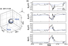 |
Fig. 1 Model–data comparisons. (a) The VEX trajectory from 6:00 to 8:00 on November 5, 2011, showing the spacecraft’s position in the VSO coordinate system. (b) A comparison of simulation results (in blue) with the VEX observations (in black) along the trajectory, with the bow-shock crossing time indicated by dashed red lines. |
Upstream solar-wind conditions for simulation cases.
3 Results
3.1 Comparison between VEX observations and MHD simulation
To validate our model calculations, we first compared the MHD simulation results with the VEX data, as depicted in Fig. 1. Figure 1a displays the VEX spacecraft’s trajectory on November 5, 2011 (orbit 2024). We extracted the simulation results along this trajectory and compared them with the measurements, as presented in Fig. 1b. The Magnetometer (MAG) observation data are shown in black, while the simulation results are depicted in blue. The simulated bow-shock crossing time closely matches the observed crossing at 07:00 UT, which is indicated by the red vertical dashed lines. Both the model results and MAG observations show a gradual increase in magnetic-field intensity between 07:00 UT and 07:17 UT as the spacecraft entered the magnetosheath and crossed the magnetic pileup boundary (MPB). The peak magnetic-field intensity in the magnetic barrier reached 230 nT in the simulation, which is comparable to the observed value of 250 nT. Around 07:50 UT, the Bx component of the magnetic field abruptly changed sign, a signature of the magnetotail’s current sheet crossing, which is reproduced by our model with a temporal offset. The good agreement between the MHD calculations and VEX data in the trends shown in all panels of Fig. 1b demonstrates that the MHD model effectively replicates many of the features observed by VEX.
3.2 Simulation results
To illustrate how the Venusian magnetic topology responded to the November 2011 ICME event, we considered three representative time points in our time-dependent simulation results: pre-ICME, ICME at five minutes, and ICME at ten minutes. These cases correspond to the quasi-steady state before the ICME, the ongoing interaction, and the new, quasi-steady state after the ICME, respectively.
Figure 2 presents three views of the model’s magnetospheric field topology during the three phases of the November 2011 ICME. In each panel, the sphere encircled by the magnetic-field lines represents the surface of Venus. The color along the magnetic-field lines indicates the magnetic-field magnitude at each point. It is evident that the magnetic fields pile up and drape around Venus. As the Bz component of the IMF increases from 0 nT to 20 nT during the ICME sheath passage, the magnetic field responds quickly with significant rotation.
To minimize the effects of directional variations in solar wind and IMF, we converted the magnetic-field data into Venus solar-electric (VSE) coordinates, as shown in Fig. 2d. In the VSE coordinates, the XVSE axis is antiparallel to the solar-wind flow, the YVSE axis aligns with the cross-flow magnetic-field component of the IMF, and the ZVSE axis is aligned with the motional electric field. The magnetic-field draping patterns in VSE coordinates are similar across the three cases, consistently with the results reported by Dimmock et al. (2018). However, there are still significant variations in the field-line draping characteristics that warrant further detailed investigation.
Magnetic topology is determined by the inferred connection points of each end of the field lines and is generally categorized in three types: closed, open, and draped, based on whether the lines connect to the ionosphere. Considering the connection to the dayside or nightside ionosphere, the topology can be further divided into six subtypes (e.g., Xu et al. 2023). However, since this study focused primarily on macroscopic variations, we did not include these further subdivisions. As seen in Fig. 3, we conducted a qualitative analysis of the broad features of magnetic topology by examining how various types of magnetic-field lines responded to the ICME event.
Based on the end points of the field lines within the model calculation domain, we classified the field lines in three categories. A field line is labeled closed (red) if both ends are anchored in the ionosphere, open (green) if one end is connected to the ionosphere while the other extends into the solar wind, and draped (blue) if both ends extend into the solar wind.
As shown in Fig. 3a, during the pre-ICME phases, all three magnetic-field-line types are present in the near-Venus space environment. The draped field lines accumulate on the dayside, and the open field lines drape around Venus, forming the magnetotail lobes. The closed field lines, potentially resulting from magnetic reconnection between the opposite-pointing open magnetic-field lines in the two lobes (e.g., Xu et al. 2024), are concentrated on the nightside. In the ICME sheath phase– shown in Figs. 3b and 3c – there is a notable increase in the occurrence of open field lines. This increased presence of open field lines is due to heightened dynamic pressure and deeper penetration of the IMF into the ionosphere. Meanwhile, the number of closed field lines gradually decreases during the ICME, which is discussed in detail in the following section. It is also worth noting that while draped field lines constitute a small proportion at low altitudes, as shown in Fig. 3, they dominate the magnetic topology at higher altitudes around Venus.
Figure 4a shows a nightside view of the area on a 300 km surface, where the model identifies regions with open, closed, or draped magnetic topologies. As previously mentioned, the areas covered by open (green) and draped (blue) fields at this low altitude expand from the pre-ICME phase to the sheath phase, indicating that IMF penetrates more deeply into the Venusian atmosphere due to enhanced dynamic pressure. Simultaneously, the closed (red) field lines gradually decrease, likely due to reduced magnetic reconnection as the direction of the magnetic field lines shifts during the ICME process.
This is also illustrated in Fig. 4b, which depicts the flaring angle of magnetic-field lines in the magnetotail at an altitude of 300 km. The flare angle, a diagnostic parameter of magnetic-field draping, is defined as the angle between the magnetic field and the Venus-Sun line, expressed as  . This angle is related to the width of the magnetotail (e.g., Crider et al. 2004). As shown in Fig. 4b, the sunward magnetic field in the +y hemisphere results in a flare angle close to 0°, while the tailward field in the -y hemisphere produces a flare angle near 180°.
As the ICME sheath progresses, it can be observed that the flare angle in the -y hemisphere gradually decreases (see Fig. 4b). This indicates that the sunward and tailward magnetic- field lines in the magnetotail are no longer antiparallel, resulting in reduced magnetic reconnection and a decline in the number of closed magnetic-field lines. Additionally, the decreasing flare angle in the -y hemisphere indicates an asymmetry between the two draped lobes. As a consequence of the lower magnetic-flux content of the tailward pointing lobe, the current sheet displaces to the right in an equilibrium configuration.
Interplanetary coronal mass ejections can substantially increase the escape rate of Venus’s ionosphere. In this study, we calculated the escape rates of  , O+, and
  during each phase of the November 2011 ICME event. The variations in the ion escape rates are summarized in Table 2. It is evident that all three planetary ion escape rates increase by an order of magnitude during the ICME event, which is consistent with previous studies on this event (e.g., McEnulty 2012). Notably, O+ shows the highest escape rate, reaching a value of 5.71 × 1026.
The escape flux of O+ ions is plotted in the X–Y plane of the VSE coordinate system to highlight this increase, as shown in Fig. 5. It is obvious that the primary escape channel is the Venusian magnetotail, which expands gradually due to the impact of the extreme event. The escape flux is influenced by both the ion number density and the radial velocity. To examine the role of magnetic topology in the increased ion escape, we analyzed the distribution of the O+ escape flux, number density, and radial velocity along the black semi-circles with radii of 2RV and 6RV in Fig. 5.
Under the influence of the ICME event, the ion density shows a slight increase during the initial interaction and then rises sharply once a new steady state is reached, while the velocity initially increases before decreasing. As illustrated in Fig. 6, the trends and peak positions of the escape flux and number density are consistent, indicating that the O+ escape flux is predominantly driven by the O+ number density. Given that solar EUV conditions remained constant during the ICME and the O+ number density in the dayside ionosphere was stable, we infer that the increase in O+ escape is due to an enhanced fraction of open magnetic-field lines that facilitate the escape.
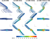 |
Fig. 2 The magnetic-topology variations during ICME passage. (a–c) Magnetic-field lines for the pre-ICME (left column) and ICME (middle and right columns) conditions in VSO coordinates. The color along the magnetic-field lines indicates the magnetic-field strength at each point. Black lines with arrows represent the direction of the magnetic field. (d) Magnetic-field data for the ICME condition in VSE coordinates. |
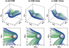 |
Fig. 3 Magnetic topology classified for pre-ICME (left column) and ICME (middle and right columns) conditions. In each case, the same field lines are traced at an altitude of 300 km. Closed field lines are shown in red, open field lines in green, and draped field lines in blue. |
Simulated escape rates of  , O+, and
  under pre-ICME and ICME conditions.
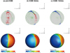 |
Fig. 4 The magnetic topology and flaring angle in the Venusian magnetotail during ICME passage. The top row shows nightside views of closed (red), open (green), and draped (blue) magnetic-field lines from Fig. 3. The bottom row depicts the flaring angle of magnetic-field lines. Time progresses from left to right. |
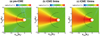 |
Fig. 5 Escape flux of O+ ions in the X–Y plane of the VSE coordinate system. The black circular lines represent the radii of 2RV and 6RV in the magnetotail. Time progresses from left to right. |
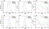 |
Fig. 6 O+ escape flux, number density, and radial velocity along the magnetotail radii of 2RV and 6RV . |
4 Discussion and conclusion
In this study, we utilized a 3D multifluid MHD model to investigate the variations in Venusian magnetic topology caused by the November 2011 ICME event. The model accounts for the production and loss of key ion species in the Venusian ionosphere, that is, H+,  , O+,
, O+,  , considering chemical reactions among these species. Its self-consistent approach to modeling both the ionosphere and the induced magnetosphere allows for a comprehensive global-scale representation of the magnetic topology in Venus’s space environment. We first validated the MHD model’s magnetic-field results by comparing them with VEX observations from November 2011, which demonstrate good agreement.
We used varying solar-wind conditions corresponding to both the pre-ICME and ICME phases to assess Venus’s timedependent response to the ICME event. By comparing our results with the hybrid simulation simulation study by Dimmock et al. (2018), which provided our input parameters, we find that our model effectively reproduces the magnetic topology patterns under extreme conditions. Our simulation indicates that while the magnetic field draping pattern during the ICME sheath phase resembles that observed under nominal solar-wind conditions, there are detailed changes in the connections and spatial orientation of the magnetic-field lines.
Magnetic topology can be categorized as closed, open, or draped, based on whether the field lines connect to the ionosphere. Our simulation results provide a detailed characterization of these magnetic topology types. Draped field lines accumulate and drape around Venus, creating the magnetic barrier and forming the magnetotail, which consists of two lobes oriented in opposite directions. Typically, draped topology dominates in the near-Venus space environment, whereas closed and open topologies are more prevalent at lower altitudes.
During the ICME event, an increase in the presence of draped fields is observed above the 300 km surface, indicating that high dynamic pressure drives draped field lines to lower altitudes. The deeper penetration of draped IMF into the ionosphere also leads to a significant increase in open field lines. In the pre-ICME phase, closed field lines are predominantly concentrated on the nightside, likely due to magnetic reconnection between the oppositely directed lobes of the magnetotail. As the ICME sheath progresses, the number of closed magnetic-field lines gradually decreases, in contrast to the increase in draped and open field lines. The flaring angle of the magnetic-field lines reveals that the sunward and tailward lobes in the magnetotail are no longer antiparallel during the ICME event, which is due to the changes in IMF direction. We infer that this shift in magnetic topology reduces magnetic reconnection, leading to a decrease in closed magnetic-field lines.
The magnetic topology has a significant impact on planetary ion escape. Open field lines, which intersect the ionosphere where ion densities are high, facilitate ion escape along these lines. In this study, we compared the O+ escape flux, number density, and radial velocity in the magnetotail escape channel. We find that the ion escape flux is primarily driven by the number density. During the ICME event, the motional electric force acting on O+ gradually increases, accompanied by a corresponding enhancement in the escape flux; this indicates an intensified escape of pickup ions.The increase in open field lines at low altitudes allows for greater ion outflow, thereby enhancing the ion escape. Additionally, it is reasonable to speculate that draped field lines, when pushed to low altitudes, may also facilitate the removal of more ions.
Moreover, we calculated the escape rates of  , O+, and
  during the November 2011 ICME event. Compared to the pre-ICME phase, the escape rates for all three ion species are increased by approximately one order of magnitude. For the same event, McEnulty (2012) estimated an O+ escape rate exceeding 2.8 × 1026 ions/s based on observed fluxes, while Dimmock et al. (2018), using a hybrid simulation, indicated an O+ escape-rate increase of over 30%. Comparing to statistical studies of Venus ICME events, Luhmann et al. (2008) identified a tenfold increase in O+ escape during one of four events analyzed, while McEnulty et al. (2010) found increased pickup ion energy but no significant flux change across ten events. Edberg et al. (2011), analyzing 157 CIR and ICME events, reported an average 1.9-fold increase in escape rates. The variability in these statistical results may be related to differences in solar activity during the analyzed periods. For Mars, Dong et al. (2015) and Ma et al. (2017) found that ion escape rates could be enhanced by an order of magnitude during the March 8, 2015 ICME event. These results suggest that ICME events can enhance ion escape at both Venus and Mars.
Given the limitations of fluid models in simulating dynamic cases, our model retains the Hall term in the generalized Ohm law, allowing for the decoupling of ion and electron motions; this better represents ion behavior under electric fields. However, it still cannot resolve the complex acceleration processes and particle trajectories that might occur during the abrupt ICME shock. Thus, the sharp transition of the ICME shock could potentially result in a more complex interaction between the solar wind and Venusian magnetic field than what is represented in our model. It is also important to note that the solar-wind input parameters used for the ICME event in this study only account for the conditions in the ICME sheath region and do not include the magnetic cloud that follows the sheath. Identifying the upstream parameters of the magnetic cloud is challenging since VEX was already located in the magnetotail at that time. Future work should explore how the magnetic topology responds to the magnetic cloud, which is characterized by smooth, large-scale rotations of the magnetic fields along with low proton density and temperature (e.g., Burlaga et al. 1981; Leamon et al. 2002). Despite these limitations, our study clearly demonstrates that the MHD model is a highly effective tool for simulating the global magnetic topology at Venus, even under disturbed conditions.
Acknowledgements
This work was supported by the B-type Strategic Priority Program of the Chinese Academy of Sciences (Grant XDB41000000), the National Natural Science Foundation of China under Grants 42241114, 42330207, 42074214, and 12150008, and the Postdoctoral Fellowship Program of CPSF under Grant GZC20233367.
References
- Bertucci, C., Mazelle, C., Slavin, J. A., Russell, C. T., & Acuña, M. H. 2003, Geophys. Res. Lett., 30, 17 [Google Scholar]
- Burlaga, L., Sittler, E., Mariani, F., & Schwenn, R. 1981, J. Geophys. Res. Space Phys., 86, 6673 [NASA ADS] [CrossRef] [Google Scholar]
- Collinson, G. A., Grebowsky, J., Sibeck, D. G., et al. 2015, J. Geophys. Res. Space Phys., 120, 3489 [CrossRef] [Google Scholar]
- Crider, D. H., Brain, D. A., Acuña, M. H., et al. 2004, Space Sci. Rev., 111, 203 [NASA ADS] [CrossRef] [Google Scholar]
- Dimmock, A. P., Alho, M., Kallio, E., et al. 2018, J. Geophys. Res. Space Phys., 123, 3580 [NASA ADS] [CrossRef] [Google Scholar]
- Dong, C., Ma, Y., Bougher, S. W., et al. 2015, Geophys. Res. Lett., 42, 9103 [NASA ADS] [CrossRef] [Google Scholar]
- Dubinin, E., Fraenz, M., Zhang, T. L., et al. 2013, J. Geophys. Res. Space Phys., 118, 7624 [NASA ADS] [CrossRef] [Google Scholar]
- Edberg, N. J. T., Nilsson, H., Futaana, Y., et al. 2011, J. Geophys. Res. Space Phys., 116, A09308 [Google Scholar]
- Forbes, T. G., Linker, J. A., Chen, J., et al. 2006, Space Sci. Rev., 123, 251 [Google Scholar]
- Fox, J. L., & Sung, K. Y. 2001, J. Geophys. Res. Space Phys., 106, 21305 [NASA ADS] [CrossRef] [Google Scholar]
- Gray, C., Chanover, N., Slanger, T., & Molaverdikhani, K. 2014, Icarus, 233, 342 [NASA ADS] [CrossRef] [Google Scholar]
- Halekas, J. S., Brain, D. A., Luhmann, J. G., et al. 2017, J. Geophys. Res. Space Phys., 122, 11320 [NASA ADS] [Google Scholar]
- Hornig, G., & Schindler, K. 1996, Phys. Plasmas, 3, 781 [NASA ADS] [CrossRef] [Google Scholar]
- Jarvinen, R., Kallio, E., Janhunen, P., et al. 2009, Annal. Geophys., 27, 4333 [CrossRef] [Google Scholar]
- Jian, L. K., Russell, C. T., Luhmann, J. G., Skoug, R. M., & Steinberg, J. T. 2008, Sol. Phys., 249, 85 [NASA ADS] [CrossRef] [Google Scholar]
- Kilpua, E., Koskinen, H. E. J., & Pulkkinen, T. I. 2017, Liv. Rev. Sol. Phys., 14, 5 [Google Scholar]
- Leamon, R. J., Canfield, R. C., & Pevtsov, A. A. 2002, J. Geophys. Res. Space Phys., 107, SSH 1 [CrossRef] [Google Scholar]
- Lillis, R. J., Brain, D. A., Bougher, S. W., et al. 2015, Space Sci. Rev., 195, 357 [NASA ADS] [CrossRef] [Google Scholar]
- Luhmann, J. G., Fedorov, A., Barabash, S., et al. 2008, J. Geophys. Res. Planets, 113, E00B04 [CrossRef] [Google Scholar]
- Luhmann, J. G., Dong, C. F., Ma, Y. J., et al. 2017, J. Geophys. Res. Space Phys., 122, 6185 [NASA ADS] [CrossRef] [Google Scholar]
- Ma, Y. J., Russell, C. T., Fang, X., et al. 2017, J. Geophys. Res. Space Phys., 122, 1714 [CrossRef] [Google Scholar]
- McComas, D. J., Spence, H. E., Russell, C. T., & Saunders, M. A. 1986, J. Geophys. Res. Space Phys., 91, 7939 [CrossRef] [Google Scholar]
- McEnulty, T. R. 2012, PhD thesis, University of California, Berkeley, USA [Google Scholar]
- McEnulty, T., Luhmann, J., de Pater, I., et al. 2010, Planet. Space Sci., 58, 1784 [NASA ADS] [CrossRef] [Google Scholar]
- Pedersen, M. N., Vanhamäki, H., Aikio, A. T., et al. 2022, J. Geophys. Res. Space Phys., 127, e2022JA030423 [CrossRef] [Google Scholar]
- Phillips, J. L., & Russell, C. T. 1987, J. Geophys. Res. Space Phys., 92, 2253 [CrossRef] [Google Scholar]
- Reva, A., Loboda, I., Bogachev, S., & Kirichenko, A. 2024, Sol. Phys., 299, 55 [NASA ADS] [CrossRef] [Google Scholar]
- Russell, C. T. 1993, Rep. Prog. Phys., 56, 687 [NASA ADS] [CrossRef] [Google Scholar]
- Ulusen, D., Luhmann, J., Ma, Y., & Brain, D. 2016, Planet. Space Sci., 128, 1 [CrossRef] [Google Scholar]
- Vech, D., Szego, K., Opitz, A., et al. 2015, J. Geophys. Res. Space Phys., 120, 4613 [CrossRef] [Google Scholar]
- Withers, P. 2009, Adv. Space Res., 44, 277 [NASA ADS] [CrossRef] [Google Scholar]
- Xu, S., Fang, X., Mitchell, D. L., et al. 2018, Geophys. Res. Lett., 45, 7337 [NASA ADS] [CrossRef] [Google Scholar]
- Xu, Q., Xu, X., Chang, Q., et al. 2019a, ApJ, 876, 84 [Google Scholar]
- Xu, S., Curry, S. M., Mitchell, D. L., et al. 2019b, J. Geophys. Res. Space Phys., 124, 151 [CrossRef] [Google Scholar]
- Xu, S., Frahm, R. A., Ma, Y., Luhmann, J. G., & Mitchell, D. L. 2021, Geophys. Res. Lett., 48, e2021GL095545 [CrossRef] [Google Scholar]
- Xu, S., Frahm, R. A., Ma, Y., et al. 2023, J. Geophys. Res. Space Phys., 128, e2023JA032133 [NASA ADS] [CrossRef] [Google Scholar]
- Xu, S., Mitchell, D. L., Whittlesey, P., et al. 2024, Nat. Commun., 15, 6065 [CrossRef] [Google Scholar]
- Zhang, T. L., Pope, S., Balikhin, M., et al. 2008, J. Geophys. Res. 113, E00B12 [Google Scholar]
All Tables
All Figures
|
Fig. 1 Model–data comparisons. (a) The VEX trajectory from 6:00 to 8:00 on November 5, 2011, showing the spacecraft’s position in the VSO coordinate system. (b) A comparison of simulation results (in blue) with the VEX observations (in black) along the trajectory, with the bow-shock crossing time indicated by dashed red lines. |
| In the text | |
|
Fig. 2 The magnetic-topology variations during ICME passage. (a–c) Magnetic-field lines for the pre-ICME (left column) and ICME (middle and right columns) conditions in VSO coordinates. The color along the magnetic-field lines indicates the magnetic-field strength at each point. Black lines with arrows represent the direction of the magnetic field. (d) Magnetic-field data for the ICME condition in VSE coordinates. |
| In the text | |
|
Fig. 3 Magnetic topology classified for pre-ICME (left column) and ICME (middle and right columns) conditions. In each case, the same field lines are traced at an altitude of 300 km. Closed field lines are shown in red, open field lines in green, and draped field lines in blue. |
| In the text | |
|
Fig. 4 The magnetic topology and flaring angle in the Venusian magnetotail during ICME passage. The top row shows nightside views of closed (red), open (green), and draped (blue) magnetic-field lines from Fig. 3. The bottom row depicts the flaring angle of magnetic-field lines. Time progresses from left to right. |
| In the text | |
|
Fig. 5 Escape flux of O+ ions in the X–Y plane of the VSE coordinate system. The black circular lines represent the radii of 2RV and 6RV in the magnetotail. Time progresses from left to right. |
| In the text | |
|
Fig. 6 O+ escape flux, number density, and radial velocity along the magnetotail radii of 2RV and 6RV . |
| In the text | |
Current usage metrics show cumulative count of Article Views (full-text article views including HTML views, PDF and ePub downloads, according to the available data) and Abstracts Views on Vision4Press platform.
Data correspond to usage on the plateform after 2015. The current usage metrics is available 48-96 hours after online publication and is updated daily on week days.
Initial download of the metrics may take a while.