| Issue |
A&A
Volume 689, September 2024
|
|
|---|---|---|
| Article Number | A214 | |
| Number of page(s) | 21 | |
| Section | Planets and planetary systems | |
| DOI | https://doi.org/10.1051/0004-6361/202450244 | |
| Published online | 13 September 2024 | |
Plasma wave survey from Parker Solar Probe observations during Venus gravity assists
1
Laboratory for Atmospheric and Space Physics, University of Colorado,
Boulder,
CO,
USA
2
Astrophysical and Planetary Sciences Department, University of Colorado,
Boulder,
CO,
USA
3
Space Sciences Laboratory, University of California, Berkeley,
Berkeley,
CA,
USA
4
Department of Physics and Astronomy, West Virginia University,
Morgantown,
WV,
USA
5
Department of Earth Planetary and Space Sciences, University of California,
Los Angeles,
CA,
USA
Received:
4
April
2024
Accepted:
22
July
2024
Abstract
Context. Parker Solar Probe (PSP) performs Venus gravity assists (VGAs) in order to lower its perihelion. PSP takes high-cadence electric and magnetic field observations during these VGAs, providing the opportunity to study plasma waves in Venus’s induced magnetosphere.
Aims. We summarize the plasma environment during these VGAs, including the regions of near-Venus space that PSP traversed and the key boundary crossings. We comprehensively identify Langmuir, ion acoustic, whistler-mode, and ion cyclotron waves during these VGAs and map the location of these waves throughout near-Venus space.
Methods. This study analyzes different data products from the PSP FIELDS instrument suite from throughout the first five VGAs.
Results. We compare the FIELDS instrumentation capabilities to the capabilities of the plasma wave instruments on board the Pioneer Venus Orbiter (PVO) and the Venus Express (VEX). We find that the PVO electric field instrument was well suited to observe Langmuir waves, especially near the bow shock and in the foreshock. However, evaluation of the other plasma waves detected by PSP FIELDS reveals that PVO and VEX would have often been unable to observe key features of these waves modes, including maximum power, bandwidth, and propagation direction. These wave characteristics provide critical information on the wave generation mechanisms and wave-particle interactions, so provide fundamental information on the nature of Venus’s induced magnetosphere.
Conclusions. These results highlight the advances in plasma wave instrumentation capabilities that have been made in the decades since the PVO and VEX eras, and illustrate the value of a plasma wave instrument on a new Venus mission.
Key words: plasmas / waves / planets and satellites: magnetic fields / planets and satellites: terrestrial planets
Corresponding author; This email address is being protected from spambots. You need JavaScript enabled to view it.
© The Authors 2024
 Open Access article, published by EDP Sciences, under the terms of the Creative Commons Attribution License (https://creativecommons.org/licenses/by/4.0), which permits unrestricted use, distribution, and reproduction in any medium, provided the original work is properly cited.
This article is published in open access under the Subscribe to Open model. This email address is being protected from spambots. You need JavaScript enabled to view it. to support open access publication.
1 Introduction
Parker Solar Probe (PSP) is a National Aeronautics and Space Administration (NASA) mission that is designed to study the solar corona, using Venus gravity assists (VGAs) to swoop closer and closer to the outer layer of the Sun. PSP’s instruments are turned on during VGAs, providing the opportunity to study the interaction between Venus and the solar wind.
Unlike Earth, Venus does not have an internal magnetic field. The magnetic environment around Venus is instead controlled by the electrodynamic interaction between ionospheric plasma and the solar wind, creating an induced magnetosphere. Venus’s induced magnetosphere drives a variety of plasma waves, summarized in reviews by Strangeway (1991) and Yadav (2021). Plasma waves can drive energy exchange between magneto-spheric particle populations (e.g., Jaynes et al. 2015) and can accelerate atmospheric particles to escape velocity and cause atmospheric loss (e.g., Ergun et al. 2006). As is discussed in Fowler et al. (2017) for the Martian induced magnetosphere, plasma waves are one mechanism by which energy transfer from the solar wind to the upper atmosphere can occur. Interactions between plasma waves and particle populations therefore play a key role in the modulation and evolution of the magnetosphere and atmosphere of a planet. Comprehensive evaluation of plasma wave activity in Venus’s induced magnetosphere (including the types of wave modes that arise, the locations where they occur, and characteristics such as amplitude and duration) is therefore necessary to understand the Venusian system and its evolution.
The most spatially comprehensive observations of plasma wave activity in Venus’s induced magnetosphere and ionosphere were predominantly made by Pioneer Venus Orbiter (PVO) and Venus Express (VEX). PVO was a NASA mission that entered Venus’s orbit on December 4, 1978 and returned data until October 1992. PVO had a polar, elliptical orbit with periap-sis near noon at an initial altitude of ~150 km (increasing to >2000 km by the end of the mission) and apoapsis in the mag-netotail at an altitude of ~12RV, where the Venus radius (RV) is 6051 km (Futaana et al. 2017). PVO carried an electric field instrument (Orbiter Electric Field Detector, OEFD) and a magnetometer (Orbiter MAGnetometer, OMAG, Russell et al. 1980). The OEFD observations were made through four continuously active channels at center frequencies of 100 Hz, 730 Hz, 5.4 kHz, and 30 kHz, with a bandwidth of ±15% of the center frequency. OMAG was a fluxgate magnetometer that was located on a 4.7 m boom and that could measure up to 12 magnetic field vectors per second. The limited coverage of the electric field spectrum and lack of high-frequency magnetic field data did not always enable conclusive identification of wave modes. For example, the 100 Hz channel observed waves that were sometimes interpreted as whistler-mode (e.g., Scarf et al. 1980), lower-hybrid (e.g., Szegö et al. 1991), or ion acoustic waves (e.g., Huba & Rowland 1993); the lack of magnetic field observations at the corresponding frequency and inability to determine wave characteristics such as bandwidth prevented conclusive identification of these plasma wave modes.
VEX was a European Space Agency (ESA) mission that entered Venus’s orbit on April 11, 2006 and operated until December 2014. Like PVO, VEX was also on a polar elliptical orbit and had a 12 RV apoapsis. However, VEX’s periapsis altitude remained at ~250–350 km throughout the mission and its periapsis was at an angle of 78°N to the ecliptic plane to enable observations of the low-altitude terminator region and mid-magnetotail around 4 RV (Zhang et al. 2006). The only plasma wave instrument carried by VEX consisted of two magnetometers (MAG, Zhang et al. 2006). One of these magnetometers was placed on the spacecraft body, while the other was located on a 1 m boom. The magnetometers had a cadence of up to 128 Hz, allowing reconstruction of waveforms up to 64 Hz (Russell et al. 2013). The lack of electric field observations meant that VEX was unable to observe any electrostatic plasma waves. However, VEX observed many whistler-mode waves over the course of its mission (Russell et al. 2007; Hart et al. 2022), as well as ion cyclotron waves (Delva et al. 2008) and 1 Hz electromagnetic waves (Xiao et al. 2020).
Other spacecraft have also observed plasma wave activity in Venus’s induced magnetosphere during VGAs. Galileo performed a VGA on February 10, 1990 and operated its plasma wave instrument for 53 minutes on the nightside of Venus near the closest approach (altitude ~ 16 000 km); it detected Lang-muir waves and electromagnetic waves at frequencies between 5–50 Hz (likely either whistler-mode or ion cyclotron waves) near the bow shock (Gurnett et al. 1991). The plasma wave instrument on board Galileo also detected nine electric field impulses that were attributed to lightning (Gurnett et al. 1991). The Cassini VGAs, which occurred on April 26, 1998 (altitude 284 km at closest approach) and June 24, 1999 (closest approach of 598 km) did not detect any signatures of lightning (Gurnett et al. 2001) but did observe Langmuir waves upstream of the Venusian bow shock (Hospodarsky et al. 2006). More recently, ESA’s Solar Orbiter performed its first VGA on December 27, 2020 entering Venus’s induced magnetosphere in the southern hemisphere of the deep magnetotail and traveling north as it approached Venus for a closest approach of 13488 km altitude over the northern pole (Hadid et al. 2021). Solar Orbiter detected whistler-mode waves, electrostatic solitary waves, ion acoustic waves and Langmuir waves in Venus’s induced magnetosphere (Hadid et al. 2021).
In this study, we examine PSP data during the first five VGAs to identify plasma wave modes, map these wave modes throughout near-Venus space, and compare key characteristics of these waves to observational capabilities of previous Venus missions. We additionally compare the spatial distribution of the different wave modes detected by PSP in near-Venus space to the distribution of these waves around Earth and Mars. This manuscript is organized as follows. Section 2 details the plasma wave instrument suite on board PSP that was used for this study. Section 3 presents an overview of the plasma environment during PSP’s first five VGAs, with further details provided in the Appendix. Section 4 presents the results and discusses the identification of Langmuir waves, ion acoustic waves, whistler-mode waves, and ion cyclotron waves. The locations where each of these wave modes were identified are mapped throughout near-Venus space. In Section 5, we discuss the plasma wave observations by PSP and their potential impacts on the broader Venusian system, and compare these to the observations and instrumentation capabilities of PVO and VEX. Section 6 concludes the study.
2 Data
PSP was launched on August 12, 2018 and performs VGAs in order to modify its orbital trajectory. Seven VGAs are planned to occur over the course of the prime mission, six of which have occurred as of today. We analyze the electric and magnetic field observations provided by the FIELDS instrument suite (PSP/FIELDS November 12, 2019; Bale et al. 2016), focusing on the first five VGAs that occurred between October 2018 and October 2021. A follow-up study is planned to analyze the plasma wave activity during VGA6 (which occurred on August 21, 2023) and VGA7 (planned for November 6, 2024) after the final VGA has been completed.
The FIELDS experiment is composed of multiple instruments. Magnetic field observations are provided by the search coil magnetometer (SCM) and two fluxgate magnetometers (FGMs); the SCM and the FGM that is used for this study are both located on a boom in PSP’s umbra. The SCM has three components (u, v, and w); all three components were functioning well in VGA1 but the SCMu component was malfunctioning from VGA2 onward. The SCM timeseries data has a sampling rate of 28/cycle in each VGA, where a cycle is defined as ~ 0.873813 s (Bale et al. 2016; Malaspina et al. 2016). The SCM also has a high-frequency component that provides magnetic field spectra from 1 kHz to 1 MHz. The FGM timeseries data had sampling rate of 28/cycle in VGAs 1, 3, 4, and 5 and a sampling rate of 27/cycle in VGA2.
Five voltage probes are included in the FIELDS instrument suite. Four of these voltage probes (V1–V4) are mounted nearly orthogonally in pairs in the plane of the heat shield, while V5 is mounted on the instrument boom. The timeseries differential voltage across pair V1 and V2 (dV12) and pair V3 and V4 (dV34) had a sampling rate of 28/cycle in VGA1 and 210/cycle in VGAs 2–5. The on board dV spectra is also provided at frequencies up to tens of MHz; the combination of the timeseries data and on board spectra enables observations of the electric field activity from DC to multi-MHz frequencies.
The PSP spacecraft coordinate system is defined with orthogonal axes, Xsc, Ysc, and Zsc. These axes are defined with +Xsc oriented in the ram direction of the spacecraft at perihelion, −Ysc is toward the ecliptic north at perihelion and +Zsc is along the long axis of PSP toward the heat shield. When the SCM and FGM data are rotated from instrument coordinates into spacecraft coordinates, these instruments provide data in the Xsc, Ysc, and Zsc directions. The pairs of voltage probes are oriented in the plane of the heat shield, so the differential voltage data are available in the XYsc plane. The Venus Solar Orbital (VSO) coordinate system defines the Venus-centered orthogonal XVSO, YVSO, and ZVSO axes. The XVSO axis corresponds to the Sun-Venus line (positive in the sunward direction), ZVSO is normal to the orbital plane, and the YVSO axis points opposite to the orbital velocity vector to complete the right-handed set.
3 Overview of Venus gravity assists
The orbital geometry of the first five VGAs provides observations throughout near-Venus space, as PSP passed through the foreshock, induced magnetosheath, induced magnetotail, and nightside ionosphere, and crossed the bow shock, induced magnetosphere boundary (IMB), and ionopause during these VGAs. Figure 1 shows the background magnetic field and PSP’s trajectory during each VGA. The background magnetic field was calculated by lowpass filtering the FGM data with a Kaiser window and cutoff frequency of 0.1 Hz. PSP’s trajectory is shown in the XYVSO plane, along with the Martinecz et al. (2009) model of the bow shock, with PSP’s location at the times of the key boundary crossings highlighted with colored dots. The Martinecz et al. (2009) bowshock model is an empirical model that is based on 19 months of VEX data; the bowshock location is relatively stable but varies with upstream solar wind and interplanetary magnetic field (IMF) conditions (Martinecz et al. 2009). Each VGA was predominantly in the XYVSO plane, with PSP only moving slightly in the ZVSO direction, so these observations are almost entirely in the equatorial plane. The trajectory of PSP during these VGAs significantly differs from the orbital coverage of PVO and VEX, which both had polar orbits, allowing observations of Venus’s induced magnetosphere where there are relatively few data. Figure B.1 shows PSP’s trajectories during all VGAs in the XYVSO and XZVSO planes, including the planned trajectory of VGA7.
The first PSP VGA occurred on October 3, 2018 with the closest approach of (0.46, −1.05, -−0.81) RV VSO at 8:44 UTC. PSP approached Venus from the nightside −YVSO sector, skimming through the turbulent magnetosheath (Bowen et al. 2021) before exiting the induced magnetosphere upstream of Venus. Figure 1a shows the background magnetic field during this VGA, and Figure 1b shows PSP’s trajectory. The bow shock crossing occurred at 8:22.29 UTC ±4 s, as is identified from the abrupt increase in the background magnetic field, which is marked by the vertical red line in Fig. 1a. PSP’s location at the best estimate time of the bow shock crossing is shown by the red dot in Fig. 1b, and this is slightly inside of the modeled bow shock location. The bow shock crossing was followed by the highly turbulent mag-netosheath region. The instruments turned off when PSP crossed the dayside/nightside boundary at ~8:42 UTC (location marked by the black dot in Fig. 1b).
VGA2 occurred on December 26, 2019 reaching its closest approach of (0.97, −1.15, −0.15) Rv at 18:15 UTC. VGA2 followed a similar trajectory to VGA1, approaching Venus from the nightside from the −YVSO direction and exiting the bow shock upstream of Venus. Figures 1c and d show the background magnetic field and PSP’s trajectory during VGA2 respectively. A partial bow shock crossing occurred at 18:06 UTC, suggesting that PSP is skimming the bow shock (Malaspina et al. 2020), followed by a complete bow shock crossing at 18:08.25 UTC ± 2 s, the best estimate timing of which is marked by the vertical red line in Figures 1c and the red dot in Figure 1d. PSP remained within the turbulent magnetosheath until it exited the bow shock at ~ 18:13.39 UTC ±2 s on the dayside of the planet, the timing of which is also marked by a red line and dot in Figures 1c and d. Both the inward and outward bow shock crossings closely align with the Martinecz et al. (2009) bow shock model. PSP then travels through the foreshock for a few minutes, as is indicated by the magnetic field turbulence upstream of the bow shock that decreases in amplitude as PSP travels further from the planet. PSP crossed a current sheet just upstream of Venus (most clearly visible in the BY rotation); PSP entered the current sheet at 18:21.00 UTC ± 30 s and exited the current sheet at 18:26.15 UTC ± 15 s. During this time, PSP traveled from (2.1, −0.20, −0.16) RV to (3.0, 0.58, −0.16) RV.
VGA3 took place on July 11, 2020, reaching its closest approach of (0.88, −0.72,0.00) RV at 3:24 UTC. The trajectory of this VGA significantly differed from VGAs 1 and 2; PSP approached Venus from the upstream −YVSO sector, passed behind the planet and exited the induced magnetosphere downstream of Venus in the +YVSO sector. The background magnetic field and trajectory during VGA3 are shown in Figures 1e and f. The turbulent foreshock can be seen as PSP approaches Venus from approximately 3:14 UTC onward, followed by the inward bow shock crossing at 3:18.19 UTC ± 2s. PSP then transited the magnetosheath and briefly entered the induced magnetosphere at 3:21.50 UTC ± 15s; the relatively large uncertainty in the IMB crossing time is due to the ambiguity in exactly when the small scale turbulence on the inner edge of the magnetosheath ended and the smoothly varying induced magnetosphere began. PSP then crossed the ionopause at 3:22.16 to enter Venus’s ionosphere, followed by the outward ionopause crossing to enter the induced magnetotail at 3:25.09 UTC (ionopause crossing times taken from Collinson et al. 2021), at which time the background magnetic field became significantly elevated from the ionospheric magnetic field and began smoothly varying. Red (orange, purple) vertical lines in Figure 1e show the bow shock (ionopause, IMB) crossings during this VGA, and dots of the same color show PSP’s location at the times that each of these boundary crossings occurred in Figure 1f. PSP was in Venus’s optical shadow from 3:22.24 to 3:33.21 UTC; the FIELDS voltage sensors reached saturation voltage within the shadow and wave activity could not be recovered from the differential timeseries data during this period. We identified the entry (exit) from Venus’s shadow from the sharp increase (decrease) in the magnitude of the voltage measured across the two pairs of voltage probes. These timings were verified using the solar panel currents, which dropped to near-zero as PSP entered the shadow and then recovered to typical levels upon exiting the shadow. At 3:34.00 UTC ±35 s, PSP left the induced magnetotail and re-entered the turbulent magnetosheath. The outward bow shock crossing occurred at 3:59.25 UTC ±4 s, identified from the sudden decrease in magnetic field magnitude, and PSP continued traveling downstream of Venus.
VGA4, which occurred on February 20, 2021, had a closest approach of (−1.18, −0.74,0.00) RV at 20:06 UTC and is shown in Figures 1g and h. The trajectory of VGA4 was very similar to VGA3, with PSP entering the induced magnetosphere from the upstream − YVSO sector, passing behind Venus and exiting the system in the downstream +YVSO direction. The inward bow shock crossing occurred at 19:58.32 UTC ±4s, as identified from the abrupt magnetic field strength increase, and then transited the magnetosheath. An 1MB crossing occurred at 20:04.00 UTC ±30 s and PSP entered the magnetotail, as identified from the change in the background magnetic field from turbulent to smooth. An ionopause crossing was not identified in this VGA, but a tail ray (filamentary extension of the ionosphere) was detected from 20:11.09 to 20:13.29 UTC (timing of tail ray crossings from Collinson et al. 2022). The outward IMB crossing then occurred at 20:15.00 UTC ± 30 s, followed by the outward bow shock crossing at 20:34.22 UTC ± 3 s. The timing of these boundary crossings and PSP’s locations are highlighted by the vertical lines in Figure 1g and dots in Figure 1h respectively, with the red lines and dots showing bow shock crossings and purple corresponding to 1MB crossings. PSP entered Venus’s optical shadow again during this VGA from 20:04.41 to 20:14.40 UTC, with shadow times identified in the same way as in VGA3; wave activity could not be recovered from the timeseries differential voltage data across the V34 pair but could be identified from the V12 timeseries data during this shadow encounter.
VGA5 occurred on October 16,2021, with a closest approach of (1.47, −0.71,0.00) RV at 9:31 UTC. PSP approached Venus from the downstream −YVSO flank (approaching on a much greater angle from the Sun-Venus line than VGAs 1 and 2) and passed in front of Venus to continue traveling slightly upstream in the +YVSO direction. Unlike the previous four VGAs, PSP did not enter Venus’s induced magnetosphere or magnetosheath in VGA5 but skimmed along the front of the subsolar bow shock. A slight increase in background magnetic field fluctuations occurred from approximately 9:05–9:55 UTC, compared to the solar wind when PSP was more distant from Venus, which may indicate that PSP was passing through Venus’s foreshock. However, no bow shock crossings were identified to indicate that PSP entered Venus’s induced magnetosphere or magnetosheath.
The differential electron energy flux obtained from the Solar Probe ANalyzer-Electron (Whittlesey et al. 2020, SPAN-E) instrument of the Solar Wind Electrons Alphas and Protons (Kasper et al. 2016; PSP/SWEAP November 12, 2019, SWEAP) suite were used to supplement the identification of these boundary crossings and plasma regions in near-Venus space. Details on these data are provided in the Appendix, and the differential electron energy flux during each VGA is shown in Figure B.2. In general, the magnetosheath had hotter electrons and elevated energy fluxes than the solar wind, which aligns with VEX electron flux observations in the magnetosheath (Martinecz et al. 2009). The ionosphere and magnetotail then had colder electrons and lower energy fluxes than both the magnetosheath and the solar wind, which again corresponds to the VEX results (Martinecz et al. 2009). The variation in electron fluxes observed by SWEAP were used to validate the timings of key boundary crossings that were primarily identified from the background magnetic field data, and supported our identification of the plasma regions of near-Venus space that PSP encountered during the VGAs.
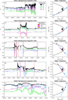 |
Fig. 1 Overview of the first five PSP VGAs. The left column shows magnitude and components (in VSO coordinates) of the magnetic field timeseries data. The right column shows PSP’s trajectory (blue) in the XYVSO plane with respect to Venus (Sun to the right) and the Martinecz et al. (2009) bow shock model (black). The best estimate times of boundary crossings are highlighted in the left column with vertical lines, and dots in the right column show PSP’s location at these times; red lines and dots correspond to bow shock crossings, purple to 1MB crossings, and orange shows ionopause crossings. The black dot in subplot b shows PSP’s location when the instruments turned off. |
4 Observations
4.1 Electrostatic wave activity
4.1.1 Langmuir waves
Langmuir waves, or electron plasma oscillations, are narrowband electrostatic plasma waves that occur around the electron plasma frequency. They are generated via the bump-on-tail instability by suprathermal electrons. At Venus, Langmuir waves have previously been identified at frequencies around multi-10’s kHz, although the frequencies that Langmuir waves arise varies with the plasma density and therefore varies between different regions of Venus’s induced magnetosphere (Hadid et al. 2021).
We use the differential voltage across the two pairs of voltage probes (dV12 and dV34) to identify the Langmuir waves. The differential voltage is obtained from both the on board voltage power spectra from the digital fields board (DFB, Malaspina et al. 2016) and the on board autospectra from the low frequency receiver (LFR) of the radio frequency spectrometer (RFS, Pulupa et al. 2017). We calculate the amplitude in units of decibels of these data by
 (1)
(1)
We defined “background” as the median differential voltage in each frequency bin during a 1–2 hour period on the day of each VGA when PSP was in the quiet solar wind and the sampling rate was sufficiently high, and “signal” as the dV data thoughout the VGA. For VGAs 1 and 2, the background field was obtained from the dV data from 2:00 to 3:00 UTC and 13:00 to 14:00 UTC respectively, when PSP was far downstream of Venus (prior to the Venus encounter) and the electric field spectra was visually quiet. In VGAs 3 and 4, the background field was calculated as the median value from 7:00 to 9:00 UTC and 22:00 to 23:59 UTC respectively, which was after the Venus encounter when PSP had returned to the quiet solar wind. The background field during VGA5 was calculated from the median values at 18:00-20:00, after the Venus encounter.
We identified potential Langmuir waves when dB > 3 at frequencies above a location-dependent threshold frequency (fthresh). The threshold frequency was set as ƒthresh = 10 kHz when PSP was located far outside Venus’s bow shock or within the induced magnetotail, and this was raised to ƒthresh = 25 kHz when PSP was near the bow shock or in the magnetosheath. When analyzing the LFR RFS data, we additionally required that the waves occurred at frequencies below 250 kHz to remove noise at the highest frequencies. This technique successfully identified all Langmuir waves that were identified by visual inspection of the spectra and minimized the number of false positives. All waves identified using this technique were then verified by eye; dust impacts (which are characterized as intense, impulsive events over a broad frequency range), noise and lower frequency ion acoustic waves (described in the next section) that extended above the threshold frequency were removed from the analysis.
Fig. 2 shows the location of all Langmuir waves that were detected in near-Venus space, and demonstrates that these waves are present throughout the different plasma regions. Langmuir waves were observed in all five of the PSP VGA’s evaluated in this study. Representative examples of the Langmuir waves detected in different regions of the induced magnetosphere are shown in Fig. 3. Many of these waves were concentrated near the bow shock, likely due to electrons reflecting off the bow shock and generating Langmuir waves in the electron foreshock. A large stream of Langmuir waves were identified as PSP skimmed across the front of the bow shock during VGA5 (Fig. 3a), and the inbound portions of VGAs 3 and 4 also detected streams of Lang-muir waves upstream from the bow shock as they approached Venus from the −YVSO sector (Fig. 3b).
Langmuir waves were also detected off the flanks of the bow shock, outside the induced magnetosphere. PSP detected clusters of Langmuir waves outside Venus’s bow shock as it approached from the downstream −YVSO sector in both VGAs 1 and 2 (Fig. 3d), and more Langmuir waves were detected outside the bow shock in the downstream dusk sectors during the outbound portions of VGAs 3 and 4. Only a handful of isolated Langmuir waves were detected within the magnetosheath, an example of which is shown in Fig. 3c, with the magnetosheath wave activity being dominated by ion acoustic waves (detailed in the next section). Langmuir waves were similarly sparse within the mag-netotail, with only a few, similarly isolated, Langmuir waves identified as PSP traversed the magnetotail during VGAs 3 and 4 (Fig. 3e). These magnetotail Langmuir waves may be driven by electron beams that were launched from magnetic reconnec-tion sites in Venus’s magnetotail, as is discussed in George et al. (2023) for Langmuir waves detected during VGA4.
4.1.2 Ion acoustic waves
Ion acoustic waves are broadband electrostatic waves that are linearly polarized and arise near the proton plasma frequency. They are generated by kinetic ion instabilities, such as the resonant interaction between counterstreaming ion populations (Gary & Omidi 1987). The motion of the spacecraft through the plasma can result in Doppler shifting of ion acoustic waves from the proton plasma frequency to higher frequencies (detailed in Mozer et al. 2020). Previous PSP observations in the solar wind identified Doppler-shifted ion acoustic waves at frequencies from 100 Hz to 10’s kHz (Mozer et al. 2020), and Doppler-shifted ion acoustic waves have also been identified in Venus’s induced magnetotail at frequencies up to ~104 Hz (an order of magnitude above the proton plasma frequency, Hadid et al. 2021).
We identified ion acoustic waves during PSP VGAs from the electric field spectra, using both the on board AC spectra and the windowed FFT of the differential voltage timeseries data. The amplitude of these data, in units of dB, were calculated and filtered in the same way as for the Langmuir waves, with the exception that the waves were identified when dB > 3 at frequencies below the threshold frequency. The threshold frequency was defined in the same way as is described in the previous section. The FIELDS data was visually inspected prior to developing the identification algorithm, and every potential ion acoustic wave had the majority (if not all) of the wave packet at frequencies below the location-dependent threshold frequency. Each wave identified by this algorithm was verified by eye to ensure the full wave packet was captured; if the wave packet extended above fthresh, the local threshold frequency was raised and the algorithm was re-run for that wave packet to ensure that the high frequency portion of the wave was captured. The highest frequency ion acoustic waves extended to an upper frequency of ~25 kHz, which occurred immediately inside the Venusian bow-shock. This frequency overlapped with the frequency of many Langmuir waves, so it was necessary to use a lower threshold frequency along with manual verification to exclude Langmuir waves from the ion acoustic wave identification. We additionally required the waves to occur at frequencies above 100 Hz when analyzing the FFT of the differential voltage timeseries data. Again, these waves were verified by eye to remove any dust strikes and noise.
The SCM data were inspected by eye during each identified wave to ensure that the waves were electrostatic, which ensured that whistler-mode waves (described in Section 4.2.1) were not mistakenly included in this portion of the analysis. We evaluated both the high frequency window of the on board AC spectra (providing magnetic field observations in the 100’s Hz – 10’s kHz range) and the FFT of the timeseries SCM data (DC – 100’s Hz). Any waves that were identified from the electric field spectra that also had a magnetic component were removed from this portion of the analysis.
Figure 4 shows examples of three waves detected by PSP during the VGAs that were identified with these criteria. The high frequency electric and magnetic field spectra are shown; the waves appear in the electric spectra but not the magnetic spectra, validating that these waves are electrostatic. The ion plasma frequency (fpi) is approximately 103 Hz in near-Venus space (Hadid et al. 2021) and the frequency of the Langmuir waves (which were always at frequencies >104 Hz) provides an estimate of the electron plasma frequency (fpe). Therefore, the waves shown in Figure 4 arise significantly below fpe but at or above fpi. As is discussed in Mozer et al. (2020), the most likely electrostatic waves that arise at these frequencies are ion acoustic waves, which may be Doppler-shifted due to the relative velocity of PSP compared to the plasma rest frame. We therefore conclude that the waves shown in Figure 4 and other waves identified with these criteria are ion acoustic waves.
Figure 5 shows the locations of ion acoustic waves throughout near-Venus space. Ion acoustic waves were detected throughout the magnetosheath on every VGA that passed through this region, indicating that magnetosheath ion acoustic waves are common at Venus. This is analogous to the 1–5 kHz waves detected at Mars (comparable frequency range to the ion acoustic waves identified at Venus) that are most abundant and most powerful within the Martian magnetosheath (Fowler et al. 2017). The 1–5 kHz waves that were concentrated in the Martian mag-netosheath overspilled through the subsolar bowshock (Fowler et al. 2017): several ion acoustic waves are also present immediately outside of the Venusian bowshock (Figure 5b). Analysis of ion acoustic waves in the solar wind found that these waves provide a substantial energy input to the particles, and may be a key component of the conversion of magnetic turbulence to particle energy (Kellogg 2020). The ubiquitous presence of ion acoustic waves in Venus’s turbulent magnetosheath may similarly drive particle energization in this region, leading to the elevated energy fluxes of magnetosheath plasma that was observed both by PSP (Figure B.2) and VEX (Martinecz et al. 2009). An example of the electric and magnetic spectra as PSP traversed the magnetosheath in VGA4 is shown in the supporting information (Figure C.1) to demonstrate the magnetosheath wave activity, which includes near-simultaneous ion acoustic, Langmuir and whistler-mode waves.
Figure 5a also shows an asymmetric distribution of ion acoustic waves outside the Venusian bow shock: the majority of the ion acoustic waves identified outside the bow shock were located in the −YVSO sector. This may be due to the Parker Spiral angle of the solar wind preferentially causing kinetic ion instabilities at the −YVSO side of the bow shock, which could then result in the ion acoustic waves generation preferentially occurring in the −YVSO sector. Ion acoustic waves were also detected within Venus’s induced magnetosphere. Figure 5b shows that ion acoustic waves were located throughout Venus’s induced mag-netotail, sometimes very close to the planet. Some ion acoustic waves were identified far upstream of Venus in VGA4; Langmuir waves were identified in a comparable location during the same VGA (Fig. 2) so it is possible that these waves are generated by backstreaming solar wind particles that reflected off Venus’s bowshock.
Electrostatic solitary waves (ESW), such as electron or ion phase space holes, arise at frequencies comparable to ion acoustic waves. ESW have previously been detected in the Venusian space environment (Malaspina et al. 2020; Hadid et al. 2021), and it is possible that our ion acoustic wave detection algorithm may also detect consecutive ESW. Unfortunately, high time resolution data is required to definitively distinguish between these wave modes and burst mode data is only sparsely available during the PSP VGAs, so we are unable to conclusively exclude ESW from our ion acoustic wave identification. Terrestrial ESW are common near the bowshock (Hansel et al. 2021), so we are most likely to mistakenly identify ESW as ion acoustic waves near Venus’s bowshock.
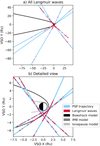 |
Fig. 2 Locations of Langmuir waves that were identified during the PSP VGAs. The PSP trajectories are all shown in light blue and the location of PSP is highlighted in red at times that Langmuir waves were identified. Subplot a shows the locations of all Langmuir waves that were identified in near-Venus space, while subplot b details the location of the waves nearest to the planet. Both subplots are in the XYVSO plane and include the Martinecz et al. (2009) bow shock model for reference. Subplot b additionally includes the models for the induced magnetosphere boundary (1MB) and ionopause from Martinecz et al. (2009). |
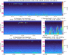 |
Fig. 3 Examples of the Langmuir waves detected in different plasma regions of near-Venus space using the DFB on board differential voltage power spectra. Subplots a, b, c and e show the dV12 data and subplot d shows the dV34 data. All subplots have the same colorscale and the subtitles give the initial and final locations of PSP in VSO coordinates over the plotted timeframes. The three pink bars on the y-axis of each subplot illustrate the frequency range of the 730 Hz, 5.4 kHz and 30 kHz channels of the PVO OEFD instrument. |
4.2 Electromagnetic wave activity
4.2.1 Whistler-mode waves
Whistler-mode waves are electromagnetic waves that are generated by mechanisms such as cyclotron resonant electron instabilities and heat-flux instabilities. They are circularly (right-hand) polarized and tend to have low wave normal angle. Whistler-mode waves typically arise at frequencies between 0.1 fce and fce. At Earth, whistler-mode waves can take the form of chorus waves (structured waves that occur in low densities, i.e., outside the plasmasphere), hiss waves (unstructured waves that arise within the plasmasphere) and lightning-generated whistler waves. Visual inspection of the FIELDS data did not reveal hiss-like waves at Venus; the whistler-mode waves detected from these data are visually similar to the chorus waves and lightning-generated whistlers that have been observed at Earth. The lack of hiss-like waves at Venus is likely because the draped structure of the induced magnetosphere is not conducive to the formation of a Venusian plasmasphere, which would require cold, dense plasma to remain trapped over long time periods. The possible generation of whistler-mode waves by lightning is a hotly debated topic (see Lorenz 2018, and references with); this study does not evaluate specific generation mechanisms of whistler-mode waves, but George et al. (2023) evaluated whistler-mode waves detected by PSP during VGA4 within the magnetotail and determined that these particular waves were not generated by lightning.
We used the timeseries SCM and differential voltage data to identify the whistler-mode waves. The SCMu component was set to 0 prior to coordinate rotation for VGAs 2–5, as this component was malfunctioning during these VGAs. The ellipticity and wave normal angle were calculated from these timeseries data via singular value decomposition (SVD) analysis (Santolík et al. 2003). The ellipticity calculated from the SCM data were then used primarily to identify the whistler-mode waves. First, we removed all ellipticity data at frequencies above 1.05 ƒce or below 0.05 ƒce. Then we masked any ellipticity values below 0.5; this meant that the filtered ellipticity data corresponded to electromagnetic and right-hand polarized data in the frequency range corresponding to whistler-mode waves. A blob-finding algorithm was then used to identify the times that coherent structures arose in the filtered ellipticity, and therefore identify the timing of potential whistler wave activity. We then verified the potential whistler-mode wave activity through visual inspection of the FFT of the timeseries SCM and dV data.
The timeseries SCM sampling rate was generally lower than the timeseries dV sampling rate, which meant that the electric spectrum was provided at higher frequencies than the magnetic spectrum. The use of SCM data to identify whistler-mode waves therefore could not have detected waves at frequencies >147 Hz (the greatest frequency that could be observed with a sampling rate of 28/cycle). However, we based our identification criteria on the SCM data in order to ensure that the waves were electromagnetic and that electrostatic waves, such as ion acoustic waves that occurred at comparable frequencies, were not mistakenly included in this portion of the analysis. This approach, while conservative, therefore ensured that every wave detected with these criteria was a whistler-mode wave. We are most likely to under-count whistler-mode waves in the magnetosheath, as this region had the highest magnetic field magnitude (see Figure 1) and therefore the highest electron cyclotron frequency, so a greater proportion of the 0.1 – 1 ƒce whistler-mode wave frequency range was above 147 Hz.
Figure 6 shows examples of whistler-mode waves identified near Venus’s bow shock, with each row corresponding to a different wave. Visually, these waves appear similar to terrestrial chorus and lightning generated whistler waves due to their structured nature (as opposed to structureless plasmaspheric hiss). The FFT of the total differential voltage data (calculated with N=2048) is shown in subplots a, d and g and the FFT of the total SCM data (N = 2048) is shown in subplots b, e and h. The ellip-ticity calculated from SCM data is shown in subplots c, f and i, with ellipticity of 1 (−1) corresponding to right-hand (left-hand) polarization and ellipticity of 0 corresponding to linear polarization. The black overlaid lines show fce and the white lines shows 0.1 fce. These examples validate that the waves identified using these criteria are electromagnetic, right-hand polarized and occur at the frequencies of 0. 1 fce − fce, so are positively identified as whistler-mode waves.
The distribution of whistler-mode waves throughout near-Venus space is shown in Figure 7. The majority of these waves were detected near the planet, especially in the magnetosheath and foreshock. Whistler-mode waves are also common near the Earth, although these inner magnetospheric whistler-mode waves generally arise in the plasmasphere (e.g., Thorne et al. 1973) and radiation belts (e.g., Cully et al. 2008); these plasma regions do not arise in Venus’s induced magnetosphere due to the draped structure of the magnetic field lines. However, whistler-mode waves also arise in the Earth’s magnetosheath (Rodriguez 1985) and upstream of the Earth’s bow shock (e.g., Zhang et al. 1998). Solar Orbiter also detected whistler waves near the outbound bow shock crossing during its VGA (Hadid et al. 2021). Detailed analysis of the Solar Orbiter observations concluded these waves were generated by electron beams and temperature anisotropies (Dimmock, A. P. et al. 2022), which also generates whistler-mode waves upstream of the Earth’s bow shock (Zhang et al. 1998). The common detection of whistler-mode waves near the bow shock by PSP indicates that these kinetic electron instabilities and resulting whistler-mode wave activity may be a common feature of Venus’s induced magnetosphere.
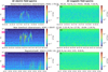 |
Fig. 4 Examples of ion acoustic waves detected in near-Venus space. Subplots a, c and e show the dV12 component of the on board AC electric field spectra. Subplots b, d and f show the on board spectra from the high-frequency window of the SCM data, validating that the waves shown in subplots a, c and e are electrostatic. Each row shows a different wave with the subtitle of each row giving the locations of PSP in VSO at the start and end of the plotted timeframes. The top and middle rows show waves detected during VGA1 and the bottom row shows a wave from VGA3. The two pink bars on the y-axes of the left subplots illustrate the frequency range of the 730 Hz and 5.4 kHz channels of the PVO OEFD instrument. |
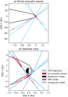 |
Fig. 5 Distribution of ion acoustic waves throughout near-Venus space, in the same format as Figure 2. |
4.2.2 Ion cyclotron waves
Ion cyclotron waves (ICW) are electromagnetic transverse waves; they are circularly (left-hand) polarized, wide bandwidth, typically have low wave normal angle and occur at frequencies near the proton cyclotron frequency (fc,H +). At Venus, ion cyclotron waves are an important signature of atmospheric loss, as hydrogen lost from the atmosphere can become ionized by solar radiation and produce the necessary ion instabilities to generate these waves (Delva et al. 2008, 2011). Analysis of ion cyclotron waves, including the locations where they occur, can therefore provide key insight to the loss of neutral hydrogen from Venus’s atmosphere.
We analyze the FGM data to identify and characterize ICWs in near-Venus space. These waves were identified through visual inspection of the magnetic power spectra, coherence, planarity, ellipticity and wave normal angle (WNA) during each of the VGAs. The planarity, ellipticity and WNA were calculated by SVD analysis of the FGM data that had been rotated into field aligned coordinates. The magnetic power spectra were calculated by taking the windowed FFT of the total FGM timeseries data with N = 214. The coherence was calculated by taking the windowed FFT of the background magnetic field data (also calculated with N = 214) and then performing cross-spectral analysis between the background field and the timeseries FGM data. This cross spectral analysis was performed across each component of the magnetic field data to obtain the coherence between the xy, xz and yz VSO components of the FGM data. The average coherence was then calculated as the mean of the coherence across these three components; when this was plotted across time and frequency, the waves often appear more distinctly than in the magnetic power spectrum where the waves are commonly obscured by noise.
Figure 8 shows examples of ICW identified in several of the VGAs. Subplots a, e, and i show the magnetic field power spectra of the FGM (calculated as a windowed FFT with N = 214) and subplots b, f, j show the average coherence of these data. Subplots c, g, k and d, h, l show the ellipticity and wave normal angle respectively, which are both calculated from the SVD analysis of the FGM data. The black line overlaid on each subplot shows fc,H+ (calculated from the background magnetic field shown in Figure 1), and the white lines in subplots a–c show the rotation frequency of the reaction wheels on board PSP. The rotation of these reaction wheels can be seen in some of the subplots (e.g., the coherent structure from 3:20 to 3:25 UTC in subplot f) but do not correspond to plasma wave activity. The colorscale of the subplots b, f, j was selected to make the waves appear prominently, with the red structures in these subplots corresponding to coherent waves. Negative ellipticity corresponds to left-hand polarization, and wave normal angle of 0° corresponds to parallel propagating waves; the blue structures in the last two columns that appear at the same time as coherent waves therefore indicate that these waves are ion-cyclotron waves.
In total, 27 ICW intervals were identified during the first five VGAs. When identifying ICW intervals, we required that 1) they had negative ellipticity (corresponding to left-hand polarization), WNA of 30° or less, and that the wave was visible in the planarity and/or coherence spectra. These waves tended to occur above the proton cyclotron frequency, which (like the ion acoustic waves) may be due to Doppler-shifting as a result of the motion of the spacecraft through the plasma rest frame.
The duration of these ICW are on the order of tens of minutes, comparable to the duration of ICW observed upstream of the Martian bowshock (Russell et al. 1990). In some cases, a series of wave packets arose in close succession, such as those shown in Figures 8a–d and i–1. We classify these successive wave packets as a single ICW interval when they occur within a few minutes of each other, so Figures 8a–d shows a single ICW interval. When there was was more than a three minute gap between wave packets, we classify each packet as a separate ICW interval. Figures 8I, j therefore shows three ICW intervals that occurred at 08:37–08:51, 09:15–09:28, and 09:40–09:46 UTC.
Some waves were identified through visual inspection of the data that had some but not all of the characteristics of ICW, such as right-hand polarization while otherwise appearing as ICW. We did not include these waves in our analysis, but expect that they are strongly Doppler-shifted ICW (as was also observed at Mercury, Schmid et al. 2021). Appendix D provides extra detail on these potentially Doppler-shifted ICW.
The locations where the ICW were detected near Venus are shown in Figure 9. These waves are distributed highly asymmetrically around Venus, with the majority of waves being detected in the −Y sector. This asymmetry reassembles the distribution of the ion acoustic waves, reinforcing the possibility that the solar wind interaction with Venus may favourably generate ion instabilities in the −Y sector.
The majority of the ICW were detected during VGAs 1 and 5. Only one ICW was detected during VGA2; this indicates that the solar wind driving conditions may have contributed to the high numbers of ICW observed during VGA1, as PSP had very similar trajectories during the first two VGAs. Venusian ICW occur more often at solar maximum than solar minimum (Delva et al. 2015) and VGA 2 occurred nearly 15 months after VGA1, which may have been long enough for solar cycle variations to significantly impact ICW generation. Multiple ICW packets were detected immediately upstream of Venus’s bowshock (Figure 9b). ICW upstream of the Martian bowshock are generated by ionized particles from the Mars hydrogen corona that create ion-ion instabilities upstream of the planet (Romanelli et al. 2016); the similarities in duration and location of the Venusian ICW indicate that these waves may have also been generated through the loss of neutral hydrogen from Venus’s atmosphere. Some of the waves detected in VGA5 were significantly upstream of Venus and their locations are not shown in Figure 9a; it is likely that these distant waves were generated purely due to solar wind processes (e.g., Jian et al. 2009) and are not related to the loss of neutral hydrogen from Venus’s atmosphere or ion instabilities related to the Venusian bow shock. Table D.1 in the appendix provides the time and location of all ICW that were identified during VGAs 1–5, including these distant waves.
 |
Fig. 6 Examples of whistler-mode waves detected near Venus, with each row showing a different wave. Subplots a, d and g show the electric field spectra calculated from the FFT of the differential voltage timeseries data, and subplots b, e and h show the FFT of the SCM timeseries data. Subplots c, f and i show the ellipticity calculated from the SCM data. The black (white) overlaid line shows fce (0.1 fce). The subtitle of each row gives the locations of PSP in VSO coordinates at the start and end of the plotted timeframes. The pink bar on the y-axes of the left subplots show the frequency coverage of the 100 Hz channel of the PVO OEFD instrument. |
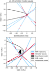 |
Fig. 7 Distribution of whistler-mode waves throughout near-Venus space, in the same format as Figure 2. |
5 Comparison to previous Venus missions
5.1 Electrostatic waves
Whenever the electric spectra from the PSP FIELDS instrument is shown (Figures 3,4,6), we have additionally illustrated the frequency coverage of the PVO OEFD instrument through pink bars on the y-axis. In some cases, the frequency coverage of an OEFD channel aligns well with the waves detected by PVO. For example, the OEFD 30 kHz channel aligns well with the Langmuir waves shown in Figure 3a and b that arose upstream of Venus’s bow shock. However, Figures 3 also provides examples of Lang-muir waves in Venus’s magnetosheath and magnetotail (subplots c and e) that occur at frequencies that are not encompassed by the OEFD 30 kHz channel. Some of the Langmuir waves in Figure 3d (downstream of Venus, outside the bow shock) also occur at frequencies that are not captured by the PVO OEFD instrument. These examples indicate that the PVO OEFD 30 kHz data are well suited to analyze the Langmuir waves in Venus’s foreshock (as was done in Crawford et al. 1990, 1993, 1998). However, we emphasize that the frequency of Langmuir waves depends on the electron density, so different solar wind conditions may result in foreshock Langmuir waves arising at frequencies that would not be captured by the PVO OEFD 30 kHz channel. The examples provided here also indicate that the PVO OEFD may underestimate the occurrence of Langmuir waves in other regions of near-Venus space. Statistical analysis of Langmuir waves at Earth showed that the majority of Langmuir waves in the magneto-tail occur near ion outflow regions of magnetic reconnection sites (Graham et al. 2023). Magnetotail reconnection at Venus is expected to occur around 1–3 RV down the tail (Zhang et al. 2006) and PSP detected Langmuir waves in this region (Fig. 2b). The Langmuir waves detected in the magnetotail during VGA4 were most likely generated by an electron beam emitted from a reconnection site (George et al. 2023). Magnetotail reconnection reshapes the system by explosively releasing energy and releasing plasmoids, and Langmuir waves in the magnetotail are a key indicator of this phenomena that have likely been undersampled by previous missions due to instrumentation limitations.
Figure 4 shows examples of ion acoustic waves detected by PSP FIELDS, which all occur over frequency ranges that overlap with the 730 Hz and/or 5.4 kHz channels of the PVO OEFD. This indicates that PVO OEFD data is suitable to detect ion acoustic waves in different regions of near-Venus space. However, the greatest power of each of these waves arises at frequencies that are not captured by either of these OEFD channels. The wave shown in Figure 4a would additionally only be detectable in the 730 Hz OEFD channel for a small portion of the total wave duration and never reached high enough frequencies to be detectable in the 5.4 kHz OEFD channel, so it would not be possible to calculate the duration or bandwidth of this wave from the PVO OEFD data. These examples provided by PSP FIELDS therefore illustrate the limitations of characterizing ion acoustic waves in terms of power, duration and bandwidth in near-Venus space using PVO OEFD data. Ion acoustic waves directly outside the Earth’s bowshock are most likely generated by ion-ion instability between the solar wind and ions reflected from the bowshock (Formisano & Torbert 1982; Goodrich et al. 2018). PSP detected several ion acoustic waves directly outside the bowshock that were likely generated by the same mechanism as at Earth. Kinetic processes (such as ion beam instabilities, Buneman instabilities, or bump-on flattop electron distributions; Akimoto & Winske 1985; Lemons & Gary 1978; Thomsen et al. 1983) generate ion acoustic waves within Earth’s bowshock, and comparable kinetic processes may have generated the abundant magnetosheath ion acoustic waves that were detected by PSP. Ion acoustic waves heat the solar wind through wave-particle interactions (Kellogg 2020) and it is likely that they play a comparable role in the magnetosheath, perhaps significantly contributing to the elevated electron energy fluxes in this region of near-Venus space (Figure B.2). Further examination of the role of ion acoustic waves in Venus’s magnetosheath and their contribution to particle energization is therefore necessary to understand the energy flow throughout the Venusian system.
In order to more thoroughly compare the PSP FIELDS instrumentation to the PVO OEFD, we compare the characteristics of the electrostatic waves detected by PSP to the statistical plasma wave analysis performed by Crawford et al. (1998). Crawford et al. (1998) evaluated the spatial distribution of the ninth decile wave intensity, which is the intensity value that 90% of observed wave intensities were less than and that 10% of wave intensities were greater than. This analysis was performed for waves detected in the 30 kHz and 5.4 kHz OEFD channels between March 8, 1986, and December 19, 1987, which spanned three Venus years (Crawford et al. 1998). We perform this comparison in aberrated IMF coordinates for two characteristic IMF orientations, based on the IMF cone angle that gives the angle between the IMF vector and solar wind velocity angle. We show these for the Parker Spiral IMF where the IMF cone angle (Ψ) is between 25° and 45° and the perpendicular IMF where 70° ≤ Ψ ≤ 90°. We calculated the average IMF as the median value of the background magnetic field in a 24 s window every 12 s and used these IMF values to rotate the PSP location from VSO to aberrated IMF coordinates, following the approach described in Section 3 of Crawford et al. (1998). We determined the IMF cone angle for each ion acoustic wave and Langmuir wave that was detected outside Venus’s bow shock and sorted these into the same IMF orientation categories as in Crawford et al. (1998). We only consider waves located outside the bow shock as we require observational data of the IMF at the time of the wave in order to accurately perform the rotation to IMF-ordered coordinates. We determined the maximum power at each timestep of these waves using the DFB AC on board spectra and binned the wave power into 0.5 × 0.5 RV bins, taking the median wave power whenever multiple datapoints fell within a single bin. The number of elements per bin for each IMF configuration is shown in Figure E.1.
Figure 10 shows the wave power of electrostatic waves detected by PSP in aberrated-IMF coordinates, overlaid on the PVO results from Crawford et al. (1998). The ion acoustic waves are shown in the left column and Langmuir waves are in the right column, with the top row showing the Parker IMF configuration and the second row showing the perpendicular IMF configuration. The PSP results in Figures 10a, b, c, and d are overlaid on Figures 2a, 1a, 5a, and 4a of Crawford et al. (1998) respectively, with the PSP data shown in reds and the figure reproductions from Crawford et al. (1998) shown with a muted rainbow col-orscale. The central frequency of the ion acoustic and Langmuir waves are shown in Figures 10e and f, binned across the frequency bins of the on board AC spectra. We define the central frequency as the frequency where the maximum wave power occurs at a given time, and consider all ion acoustic and Lang-muir waves detected throughout the VGAs (not just those outside the bow shock). The pink bars on the x-axes of Figures 10e and f show the frequency coverage of the 730 Hz, 5.4 kHz and 30 kHz PVO OEFD channels. We show these results for data recorded across the V1 and V2 pair to avoid double counting waves that were observed across both voltage probe pairs, but the results from dV34 are very similar.
The Langmuir waves detected by PSP in the electron fore-shock closely correspond to the wave intensity distribution in the 30 kHz OEFD channel reported by Crawford et al. (1998). In the Parker configuration, PSP detected Langmuir waves that fell on a diagonal line that almost exactly overlaps with the region of greatest wave intensity detected by the 30 kHz OEFD channel. The most powerful Langmuir waves detected by PSP in the Parker configuration occurred in the foreshock very near to Venus and the wave power decreased further from the planet, which corresponds well 30 kHz OEFD observations. When the IMF was in the perpendicular orientation, the Langmuir wave power was generally lower than for the Parker IMF configuration (consistent with Crawford et al. 1998). PSP detected a stream of Langmuir waves off Venus’s bow shock in the perpendicular IMF configuration, which approximately aligns with the region where the most intense 30 kHz waves were detected. The central frequency of the Langmuir waves detected by PSP forms a quasi-Gaussian distribution that peaks around 30 kHz. This analysis demonstrates that the 30 kHz channel of the PVO OEFD was well suited to detecting and analyzing Langmuir waves in near-Venus space. As is discussed in Greenstadt et al. (1995), the Earth’s electron foreshock has similar Langmuir waves as observed by PVO at Venus, although on a much larger spatial scale (approximately 14 to 1 when scaling by the bow shock size). Our results validate that data from the 30 kHz OEFD channel is well suited to analyze the Langmuir wave activity in the electron foreshock and determine the spatial extent and variation in the Venusian electron foreshock.
The majority of the ion acoustic waves detected by PSP were located within Venus’s magnetosheath, so Figures 10a and c shows relatively few waves. However, when the IMF is in the Parker configuration, the ion acoustic waves detected by PSP outside the bow shock all arose very near to the bow shock in a region where Crawford et al. (1998) reported elevated wave power in the 5.4 kHz OEFD channel. PSP detected more ion acoustic waves outside the bow shock when the IMF was in a perpendicular configuration, and these waves all had comparable power. This corresponds to the Crawford et al. (1998) results that reported fairly uniform wave intensity outside the bow shock in the 5.4 kHz channel for perpendicular IMF. The central frequencies of the ion acoustic waves show a much greater spread than the Langmuir waves. The sharp cut-off at 366 Hz in Figure 10e is a result of the broadband distribution of magnetosheath ion-acoustic waves that typically extended to frequencies below lowest frequency of the on board AC spectra (example shown in Figure C.1). Ion acoustic waves at these low frequencies are detected with the FFT of the dV timeseries data; we only show the results from the on board AC spectra in Figure 10 because the timesteps from these two datasets are different and do not allow one-to-one comparison. The majority of the ion acoustic waves that extended to frequencies below the DFB AC spectra frequency range occurred in the magnetosheath, so Figure 10 accurately represents the wave power outside the bow shock. The broad central frequency distribution of the ion acoustic waves meant that neither the 730 Hz or 5.4 kHz OEFD channel was able to capture a significant proportion of the ion acoustic waves. The 100 Hz OEFD channel could have captured some of the lower frequency ion acoustic waves in the magnetosheath, but the lack of simultaneous magnetic field observations at these frequencies means that it would not have been possible to distinguish whistler-mode and ion acoustic waves from PVO data; Figure C.1 shows that both these wave modes were present at comparable frequencies in the magnetosheath. This analysis demonstrates that the PVO OEFD instrument was severely hampered in its ability to detect, conclusively identify, and analyze ion acoustic waves in and near Venus’s induced magnetosphere.
 |
Fig. 8 Examples of ion cyclotron waves identified during the Parker Solar Probe Venus gravity assists. Each wave is shown in a different row, with the columns corresponding to the magnetic power spectra (a, e, i), average coherence (b, f, j), ellipticity (c, g, k), and wave normal angle (d, h, l). The overlaid black lines show the proton cyclotron frequency, and the white lines in subplots a–c show the rotation wheel frequency. Times are provided in UTC. |
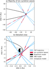 |
Fig. 9 Distribution of ion cyclotron waves throughout near-Venus space, in the same format as Figure 2. Some waves that were detected during VGA5 are not shown in subplot a as they were large distances away from Venus, but Table D.1 in the appendix provides the times and locations where all ICW were detected. |
5.2 Electromagnetic waves
Examples of whistler-mode waves are shown in Fig. 6 and compared to the frequency coverage of the 100 Hz OEFD channel. While some of the whistler-mode waves shown here would be detectable by PVO OEFD, such as in Figure 6g or Figure 6a after the bow shock crossing, the waves shown in Figure 6d and Figure 6a prior to the bow shock crossing would not be detectable with this instrument. Some of these low frequency electromagnetic waves would have been detectable with the VEX magnetometer that could detect waveforms up to 64 Hz. However, neither PVO nor VEX had the instrumentation capabilities to observe both the electric and magnetic components of the whistler-mode waves, which is necessary to calculate the directional Poynting flux. At Mars, Poynting flux calculations have been used to evaluate the propagation of waves that were generated in the magne-tosheath into the upper ionosphere (Fowler et al. 2017). We have demonstrated that whistler-mode waves arise in Venus’s magnetosheath (particularly in the − Y sector, Figure 7) and it is possible that these magnetosheath waves may propagate into Venus’s ionosphere as they do at Mars; indeed, PVO and VEX have detected many whistler-mode waves in Venus’s ionosphere (e.g., Russell et al. 1989; Hart et al. 2022). Venus’s ionospheric whistler waves are often attributed to lightning, although this interpretation is not universally accepted by the scientific community (see Lorenz 2018, and references within). Evaluation of the Poynting flux of whistler-mode waves detected in the magnetotail during PSP VGA4 enabled George et al. (2023) to eliminate lightning as a generation mechanism of these waves, which was only possible due to the simultaneous observations of the electric and magnetic field by the FIELDS instrument. Calculation of the Poynting flux of whistler-mode waves is therefore necessary to conclusively identify the generation mechanism of whistler-mode waves in Venus’s ionosphere, and distinguish between waves generated in magnetosheath or magnetotail that propagate into the ionosphere and those that are generated by lightning within Venus’s ionosphere.
Ion cyclotron waves arise at frequencies significantly lower than the frequency coverage of OEFD. The lowest frequency channel on OEFD was 100 Hz and the examples of ion cyclotron waves shown in Figure 8 occur at frequency range of 10−1– 101 Hz; all ion cyclotron waves detected by PSP during VGAs 1–5 occurred at comparable frequencies. However, while it was not possible for OEFD to detect ion cyclotron waves, the magnetometer on board PVO (OMAG) was capable of detecting these waves. Russell et al. (2006) reported observations of ion cyclotron waves in Venus’s magnetosheath from OMAG, and the magnetometer on board VEX was also capable of detecting these waves (e.g., Delva et al. 2008). At Mars, upstream ion cyclotron waves are most likely generated by protons formed by the ionization of the neutral Martian hydrogen corona, and the subsequent ion-ion instabilities that form between these pickup ions and the solar wind (Bertucci et al. 2013; Romanelli et al. 2016). PSP detected multiple ion cyclotron wave packets immediately outside the subsolar bow shock (Fig. 9b), which may have similarly been generated through the loss of neutral hydrogen (Delva et al. 2011). The composition and evolution of planetary atmospheres is fundamentally tied to the escape of atmospheric particles, particularly hydrogen (Delva et al. 2011), so analysis of the occurrence rates and generation mechanisms of ion cyclotron waves at Venus will enable more precise understanding of the Venusian atmosphere.
Finally, we note that not every wave mode that arises in Venus’s induced magnetosphere was included in this study. For example, electrostatic solitary waves (ESW) have also been detected by PSP during VGAs (Malaspina et al. 2020) and by Solar Orbiter during its first VGA (Hadid et al. 2021). We did not evaluate ESW in this study as they can only be detected from the DFB burst data, and this burst data is only sparsely available throughout the VGAs. The sparse data availability meant that we could not conclusively identify and map ESW throughout near-Venus space in the same way that was done for other plasma wave modes in this study, so ESW were not included in this analysis.
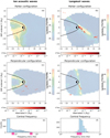 |
Fig. 10 Subplot a shows the maximum power of the ion acoustic waves detected by PSP (red colorscale) when the IMF was in the Parker configuration, overlaid on Figure 2a of Crawford et al. (1998) (muted rainbow colorscale). Subplot b shows the same but for the Langmuir waves detected by PSP overlaid on Figure 1a of Crawford et al. (1998). Subplots c and d show the ion acoustic and Langmuir waves respectively when the solar wind was in a perpendicular configuration, overlaid on Figures 5a and 4a of Crawford et al. (1998) respectively. The bow shock calculated from the Martinecz et al. (2009) model is shown in black in subplots a–d. Subplots e and f show the central frequency of all the ion acoustic and Langmuir waves detected by PSP respectively. The pink bars on the x-axis of subplots e and f show the frequency coverage of channels of the PVO OEFD instrument. |
6 Conclusion
We have presented an overview of the Langmuir waves, ion acoustic waves, whistler-mode waves, and ion cyclotron waves detected by PSP during VGAs 1–5. Representative examples of each of these waves have been plotted in various regions of Venus’s induced magnetosphere, and the locations where these waves were identified have been mapped throughout near-Venus space. Plasma waves provide key information on fundamental magnetospheric and atmospheric processes, such as kinetic instabilities, particle energization, energy input to the ionosphere, and the possible occurrence of lightning. Long-term, dedicated observations of plasma waves in near-Venus space are therefore necessary to understand particle dynamics in the Venusian system and the energy flow through near-Venus space.
We performed this analysis using FIELDS data provided by PSP during VGAs. We compared these observations to the instrumentation capabilities of previous Venus missions: specifically the OEFD and OMAG of PVO and the magnetometer on board VEX. PVO was launched in 1978 and the OEFD instrument on board this mission provides the only long-term, dedicated observations of electric field plasma wave activity at Venus. The PSP FIELDS data reveals the advances in plasma wave instrumentation that have occurred in the 50 years since the PVO OEFD, and highlights the value of simultaneous electric and magnetic field observations over a comprehensive frequency range. The PSP FIELDS instrument, unlike the previous instruments on board PVO and VEX, provides the data necessary to conclusively identify wave modes and identify features such as the maximum power, bandwidth, and propagation direction. These results highlight the value of a modern plasma wave instrument on a Venus mission to more accurately detect and analyze various plasma waves throughout Venus’s induced magnetosphere. More thorough understanding of these plasma waves, their characteristics, and the locations where they arise will inform us on the nature of Venus’s induced magnetosphere and the solar wind-ionosphere interaction that occurs at Venus.
Acknowledgements
This work was enabled by NASA grant number 80NSSC21K2019. LCG was supported by NASA award 80NSSC21K1386. Parker Solar Probe was designed, built, and is now operated by the Johns Hopkins Applied Physics Laboratory as part of NASA’s Living with a Star (LWS) program (contract NNN06AA01C). Support from the LWS management and technical team has played a critical role in the success of the Parker Solar Probe mission.
Appendix A Introduction
This appendix provides additional details and context for the Parker Solar Probe (PSP) Venus gravity assists (VGAs). It also includes further examples of plasma wave activity detected in the magnetosheath of Venus’s induced magnetosphere, as detected by the FIELDS instrument on board PSP, and catalogues each ion cyclotron wave identified in VGAs 1-5.
Appendix B Extended overview of PSP Venus gravity assists
Figure B.1 provides a summary of PSP’s trajectory during the Venus gravity assists in the XY and XZ planes of the VSO coordinate system. The actual trajectories of PSP during VGAs 1 - 6 are shown along with the planned trajectory of VGA7, which has not been completed as of the writing of this manuscript. These trajectories are shown in relation to the Martinecz et al. (2009) conic bow shock model.
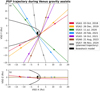 |
Fig. B.1 Overview of the Parker Solar Probe trajectories during the Venus gravity assists in the VSO coordinate frame. Subplot a shows the trajectories in the VSO XY plane and subplot b shows these in the VSO XZ plane; the Sun is to the right in both subplots and the black line represents the conic bow shock model from Martinecz et al. (2009). |
Figure B.2 shows a detailed overview of each VGA, in the same format as in Figure 1 but with the differential electron energy flux in the left column instead of the background magnetic field. The differential electron energy flux is obtained from the Solar Probe ANalyzer-Electron (SPAN-E Whittlesey et al. 2020) instrument of the Solar Wind Electrons Alphas and Protons (SWEAP Kasper et al. 2016; PSP/SWEAP November 12, 2019) suite. We use the level 3 data product that provides the differential electron energy flux versus energy; during each VGA, the electron energy range was 2.04 – 1,794 eV. In VGA1, the temporal cadence of these data were 28 s and the temporal cadence of these data were 14 s in VGAs 2-5. Vertical lines are overlaid on Figure B.2 a, c, e, g, and i to highlight when PSP crossed a boundary of Venus’s induced magnetosphere (red lines for bow shock crossings, purple lines for induced magnetosphere boundary crossings, and orange for the ionopause crossings). Dots are placed on the trajectory plots (Fig B.2 b, d, f, h, j) to show PSP’s location at the times of these boundary crossing, with the same color used for the dots as for the vertical lines.
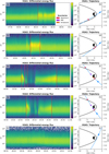 |
Fig. B.2 Overview of the first five PSP VGAs; analogous to Figure 1 in the main text but with the left column showing differential electron energy flux. The same colorscale is used for each subplot in the left column. The right column again shows PSP’s trajectory (blue) in the VSO XY plane with respect to Venus (Sun to the right) and the Martinecz et al. (2009) bow shock model (black). The best estimate times of boundary crossings are highlighted in the left column with vertical lines, and dots in the right column show PSP’s location at these times; red lines and dots correspond to bow shock crossings, purple to IMB crossings, and orange shows ionopause crossings. The black dot in subplot b shows PSP’s location when the instruments turned off. |
Appendix C Magnetosheath wave activity
Figure C.1 shows an example of the magnetosheath wave activity from the inbound magnetosheath crossing of VGA4. Subplot a shows the on board AC spectra across the V12 pair and subplot b shows the high frequency window of the SCM data. Subplot c shows the fast Fourier transform (FFT) of the total differential voltage recorded across both the V12 and V34 pair (calculated with N = 2048) and subplot d shows the FFT of the total magnetic field recorded by the SCM, which was calculated with N = 1024.
Figure C.1 demonstrates the highly active nature of Venus’s induced magnetosheath, with multiple plasma wave modes detected within a few minutes. A Langmuir wave with f ~ 3 × 10⁴ Hz was identified immediately before the inward bow shock crossing. Directly after the bow shock crossing, a several-minute long stream of ion acoustic waves were detected across a broad frequency range of ~102 − 104 Hz. The FFT of the SCM timeseries data reveals a series of whistler waves throughout the magnetosheath, some of which were simultaneous with the ion acoustic waves but occurred at lower frequencies (~10′ s Hz, below the electron cyclotron frequency).
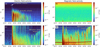 |
Fig. C.1 Plasma wave activity throughout the magnetosheath during the inbound portion of VGA4, which includes Langmuir, ion acoustic and whistler−mode waves. Subplot a shows the on board AC electric field spectra across the V12 voltage probe pair, subplot b shows the high frequency window of the SCM magnetic field data, c shows the FFT of the total differential voltage timeseries data, and subplot d shows the FFT of the total SCM timeseries data. |
Appendix D List of identified ion cyclotron waves
Table D.1.1 lists the time and location of all ion cyclotron waves that were identified by PSP in VGAs 1-5. Times are given in UTC and the VGA that a given wave was observed during is provided in the left column. The start and end times of the ICW are given to one-minute precision, and the right two columns give the locations of PSP at the wave start time and the wave end time in VSO coordinates.
Some waves were identified that had some, but not all, of the properties that we required for identification of ion cyclotron waves. These waves may be Doppler-shifted ion cyclotron waves, and the timing and location of these waves are provided in Table D.2.2. Figure D.1 provides the location of these waves, in the same format as for Figure 9.
Appendix E Data density
Figure E.1 shows the number of elements in each 0.5 × 0.5RV bin that was evaluated for Figure 10 of the main text. Subplot a shows the Parker configuration that corresponds to interplanetary magnetic field (IMF) cone angles between 25° and 45°, and subplot b shows the perpendicular configuration that corresponds to IMF cone angles between 70° and 90°. These results are shown in aberrated-IMF coordinates.
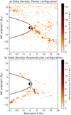 |
Fig. E.1 Number of elements per bin for the two interplanetary mag netic field configurations considered for Figure 10 of the main text. The conic bow shock model from Martinecz et al. (2009) is shown in black. |
Time and location of ion cyclotron waves identified by PSP during VGAs 1−5.
Time and location of possibly Doppler−shifted ion cyclotron waves identified by PSP during VGAs 1–5.
References
- Akimoto, K., & Winske, D. 1985, J. Geophys. Res.: Space Phys., 90, 12095 [NASA ADS] [CrossRef] [Google Scholar]
- Bale, S. D., Goetz, K., Harvey, P. R., et al. 2016, Space Sci. Rev., 204, 49 [Google Scholar]
- Bertucci, C., Romanelli, N., Chaufray, J. Y., et al. 2013, Geophys. Res. Lett., 40, 3809 [NASA ADS] [CrossRef] [Google Scholar]
- Bowen, T. A., Bale, S. D., Bandyopadhyay, R., et al. 2021, Geophys. Res. Lett., 48, e2020GL090783 [Google Scholar]
- Collinson, G. A., Ramstad, R., Glocer, A., Wilson III, L., & Brosius, A. 2021, Geophys. Res. Lett., 48, e2020GL092243 [CrossRef] [Google Scholar]
- Collinson, G. A., Ramstad, R., Frahm, R., et al. 2022, Geophys. Res. Lett., 49, e2021GL096485 [CrossRef] [Google Scholar]
- Crawford, G. K., Strangeway, R. J., & Russell, C. T. 1990, Geophys. Res. Lett., 17, 1805 [Google Scholar]
- Crawford, G. K., Strangeway, R. J., & Russell, C. T. 1993, Geophys. Res. Lett., 20, 2801 [NASA ADS] [CrossRef] [Google Scholar]
- Crawford, G. K., Strangeway, R. J., & Russell, C. T. 1998, J. Geophys. Res.: Space Phys., 103, 11985 [NASA ADS] [CrossRef] [Google Scholar]
- Cully, C. M., Bonnell, J. W., & Ergun, R. E. 2008, Geophys. Res. Lett., 35, L17S16 [NASA ADS] [CrossRef] [Google Scholar]
- Delva, M., Zhang, T. L., Volwerk, M., et al. 2008, Geophys. Res. Lett., 35, L03105 [NASA ADS] [CrossRef] [Google Scholar]
- Delva, M., Mazelle, C., & Bertucci, C. 2011, Space Sci. Rev., 162, 5 [Google Scholar]
- Delva, M., Mazelle, C., Bertucci, C., et al. 2011, J. Geophys. Res.: Space Phys., 116, 5 [Google Scholar]
- Delva, M., Bertucci, C., Volwerk, M., et al. 2015, J. Geophys. Res.: Space Phys., 120, 344 [NASA ADS] [CrossRef] [Google Scholar]
- Dimmock, A. P., Khotyaintsev, Yu. V., Lalti, A., et al. 2022, A&A, 660, A64 [NASA ADS] [CrossRef] [EDP Sciences] [Google Scholar]
- Ergun, R. E., Andersson, L., Peterson, W. K., et al. 2006, Geophys. Res. Lett., 33, L14103 [NASA ADS] [CrossRef] [Google Scholar]
- Formisano, V., & Torbert, R. 1982, Geophys. Res. Lett., 9, 207 [NASA ADS] [CrossRef] [Google Scholar]
- Fowler, C. M., Andersson, L., Halekas, J., et al. 2017, J. Geophys. Res.: Space Phys., 122, 8536 [NASA ADS] [CrossRef] [Google Scholar]
- Futaana, Y., Stenberg Wieser, G., Barabash, S., & Luhmann, J. G. 2017, Space Sci. Rev., 212, 1453 [NASA ADS] [CrossRef] [Google Scholar]
- Gary, S. P., & Omidi, N. 1987, J. Plasma Phys., 37, 45 [CrossRef] [Google Scholar]
- George, H., Malaspina, D. M., Goodrich, K., et al. 2023, Geophys. Res. Lett., 50, e2023GL105426 [NASA ADS] [CrossRef] [Google Scholar]
- Goodrich, K. A., Ergun, R., Schwartz, S. J., et al. 2018, J. Geophys. Res.: Space Phys., 123, 9430 [NASA ADS] [CrossRef] [Google Scholar]
- Graham, D. B., Khotyaintsev, Y. V., & André, M. 2023, J. Geophys. Res.: Space Phys., 128, e2023JA031900 [NASA ADS] [CrossRef] [Google Scholar]
- Greenstadt, E. W., Crawford, G. K., Strangeway, R. J., Moses, S. L., & Coroniti, F. V. 1995, J. Geophys. Res.: Space Phys., 100, 19933 [NASA ADS] [CrossRef] [Google Scholar]
- Gurnett, D. A., Kurth, W. S., Roux, A., et al. 1991, Science, 253, 1522 [NASA ADS] [CrossRef] [Google Scholar]
- Gurnett, D. A., Zarka, P., Manning, R., et al. 2001, Nature, 409, 313 [NASA ADS] [CrossRef] [Google Scholar]
- Hadid, L. Z., Edberg, N. J. T., Chust, T., et al. 2021, A&A, 656, A18 [NASA ADS] [CrossRef] [EDP Sciences] [Google Scholar]
- Hansel, P. J., Wilder, F. D., Malaspina, D. M., et al. 2021, J. Geophys. Res.: Space Phys., 126, e2021JA029389 [CrossRef] [Google Scholar]
- Hart, R. A., Russell, C. T., & Zhang, T. 2022, Icarus, 380, 114993 [CrossRef] [Google Scholar]
- Hospodarsky, G. B., Kurth, W. S., Gurnett, D. A., et al. 2006, Planetary Radio Emissions VI, in Proceedings of the 6th International Workshop held at Graz, 67 [Google Scholar]
- Huba, J. D., & Rowland, H. L. 1993, J. Geophys. Res.: Planets, 98, 5291 [NASA ADS] [CrossRef] [Google Scholar]
- Jaynes, A. N., Baker, D. N., Singer, H. J., et al. 2015, J. Geophys. Res.: Space Phys., 120, 7240 [NASA ADS] [CrossRef] [Google Scholar]
- Jian, L. K., Russell, C. T., Luhmann, J. G., et al. 2009, ApJ, 701, L105 [CrossRef] [Google Scholar]
- Kasper, J. C., Abiad, R., Austin, G., et al. 2016, Space Sci. Rev., 204, 131 [Google Scholar]
- Kellogg, P. J. 2020, ApJ, 891, 51 [CrossRef] [Google Scholar]
- Lemons, D. S., & Gary, S. P. 1978, J. Geophys. Res.: Space Phys., 83, 1625 [NASA ADS] [CrossRef] [Google Scholar]
- Lorenz, R. D. 2018, Progr. Earth Planet. Sci., 5, 34 [NASA ADS] [CrossRef] [Google Scholar]
- Malaspina, D. M., Ergun, R. E., Bolton, M., et al. 2016, J. Geophys. Res.: Space Phys., 121, 5088 [NASA ADS] [CrossRef] [Google Scholar]
- Malaspina, D. M., Goodrich, K., Livi, R., et al. 2020, Geophys. Res. Lett., 47, e2020GL090115 [CrossRef] [Google Scholar]
- Martinecz, C., Boesswetter, A., Fränz, M., et al. 2009, J. Geophys. Res.: Planets, 114, 00B30 [Google Scholar]
- Mozer, F. S., Bonnell, J. W., Bowen, T. A., Schumm, G., & Vasko, I. Y. 2020, ApJ, 901, 107 [NASA ADS] [CrossRef] [Google Scholar]
- PSP/FIELDS. November 12, 2019, PSP/FIELDS online data repository, [Dataset]. Accessed: 10 August 2023 [Google Scholar]
- PSP/SWEAP. November 12, 2019, PSP/SWEAP online data repository, [Dataset]. Accessed: 10 August 2023 [Google Scholar]
- Pulupa, M., Bale, S. D., Bonnell, J. W., et al. 2017, J. Geophys. Res.: Space Phys., 122, 2836 [NASA ADS] [CrossRef] [Google Scholar]
- Rodriguez, P. 1985, J. Geophys. Res.: Space Phys., 90, 6337 [NASA ADS] [CrossRef] [Google Scholar]
- Romanelli, N., Mazelle, C., Chaufray, J. Y., et al. 2016, J. Geophys. Res.: Space Phys., 121, 11,113 [NASA ADS] [CrossRef] [Google Scholar]
- Russell, C. T., Snare, R. C., Means, J. D., & Elphic, R. C. 1980, IEEE Trans. Geosci. Remote Sens., GE-18, 32 [CrossRef] [Google Scholar]
- Russell, C. T., von Dornum, M., & Strangeway, R. J. 1989, Geophys. Res. Lett., 16, 579 [NASA ADS] [CrossRef] [Google Scholar]
- Russell, C. T., Luhmann, J. G., Schwingenschuh, K., Riedler, W., & Yeroshenko, Y. 1990, Geophys. Res. Lett., 17, 897 [NASA ADS] [CrossRef] [Google Scholar]
- Russell, C., Mayerberger, S., & Blanco-Cano, X. 2006, Adv. Space Res., 38, 745 [NASA ADS] [CrossRef] [Google Scholar]
- Russell, C. T., Zhang, T. L., Delva, M., et al. 2007, Nature, 450, 661 [CrossRef] [Google Scholar]
- Russell, C. T., Leinweber, H., Zhang, T. L., et al. 2013, Geophys. Res. Lett., 40, 216 [NASA ADS] [CrossRef] [Google Scholar]
- Santolík, O., Parrot, M., & Lefeuvre, F. 2003, Radio Sci., 38, 1010 [Google Scholar]
- Scarf, F. L., Taylor, W. W. L., Russell, C. T., & Brace, L. H. 1980, J. Geophys. Res.: Space Phys., 85, 8158 [NASA ADS] [CrossRef] [Google Scholar]
- Schmid, D., Narita, Y., Plaschke, F., et al. 2021, Geophys. Res. Lett., 48, e2021GL092606 [CrossRef] [Google Scholar]
- Strangeway, R. J. 1991, Space Sci. Rev., 55, 275 [CrossRef] [Google Scholar]
- Szegö, K., Shapiro, V. S., Shevchenko, V. I., et al. 1991, Geophys. Res. Lett., 18, 2305 [CrossRef] [Google Scholar]
- Thomsen, M. F., Barr, H. C., Gary, S. P., Feldman, W. C., & Cole, T. E. 1983, J. Geophys. Res.: Space Phys., 88, 3035 [NASA ADS] [CrossRef] [Google Scholar]
- Thorne, R. M., Smith, E. J., Burton, R. K., & Holzer, R. E. 1973, J. Geophys. Res., 78, 1581 [NASA ADS] [CrossRef] [Google Scholar]
- Whittlesey, P. L., Larson, D. E., Kasper, J. C., et al. 2020, ApJS, 246, 74 [Google Scholar]
- Xiao, S., Wu, M., Wang, G., Chen, Y., & Zhang, T. 2020, Planet. Space Sci., 187, 104933 [CrossRef] [Google Scholar]
- Yadav, V. K. 2021, IETE Tech. Rev., 38, 622 [CrossRef] [Google Scholar]
- Zhang, T., Baumjohann, W., Delva, M., et al. 2006, Planet. Space Sci., 54, 1336 [NASA ADS] [CrossRef] [Google Scholar]
- Zhang, Y., Matsumoto, H., & Kojima, H. 1998, J. Geophys. Res.: Space Phys., 103, 20529 [NASA ADS] [CrossRef] [Google Scholar]
All Tables
Time and location of possibly Doppler−shifted ion cyclotron waves identified by PSP during VGAs 1–5.
All Figures
|
Fig. 1 Overview of the first five PSP VGAs. The left column shows magnitude and components (in VSO coordinates) of the magnetic field timeseries data. The right column shows PSP’s trajectory (blue) in the XYVSO plane with respect to Venus (Sun to the right) and the Martinecz et al. (2009) bow shock model (black). The best estimate times of boundary crossings are highlighted in the left column with vertical lines, and dots in the right column show PSP’s location at these times; red lines and dots correspond to bow shock crossings, purple to 1MB crossings, and orange shows ionopause crossings. The black dot in subplot b shows PSP’s location when the instruments turned off. |
| In the text | |
|
Fig. 2 Locations of Langmuir waves that were identified during the PSP VGAs. The PSP trajectories are all shown in light blue and the location of PSP is highlighted in red at times that Langmuir waves were identified. Subplot a shows the locations of all Langmuir waves that were identified in near-Venus space, while subplot b details the location of the waves nearest to the planet. Both subplots are in the XYVSO plane and include the Martinecz et al. (2009) bow shock model for reference. Subplot b additionally includes the models for the induced magnetosphere boundary (1MB) and ionopause from Martinecz et al. (2009). |
| In the text | |
|
Fig. 3 Examples of the Langmuir waves detected in different plasma regions of near-Venus space using the DFB on board differential voltage power spectra. Subplots a, b, c and e show the dV12 data and subplot d shows the dV34 data. All subplots have the same colorscale and the subtitles give the initial and final locations of PSP in VSO coordinates over the plotted timeframes. The three pink bars on the y-axis of each subplot illustrate the frequency range of the 730 Hz, 5.4 kHz and 30 kHz channels of the PVO OEFD instrument. |
| In the text | |
|
Fig. 4 Examples of ion acoustic waves detected in near-Venus space. Subplots a, c and e show the dV12 component of the on board AC electric field spectra. Subplots b, d and f show the on board spectra from the high-frequency window of the SCM data, validating that the waves shown in subplots a, c and e are electrostatic. Each row shows a different wave with the subtitle of each row giving the locations of PSP in VSO at the start and end of the plotted timeframes. The top and middle rows show waves detected during VGA1 and the bottom row shows a wave from VGA3. The two pink bars on the y-axes of the left subplots illustrate the frequency range of the 730 Hz and 5.4 kHz channels of the PVO OEFD instrument. |
| In the text | |
|
Fig. 5 Distribution of ion acoustic waves throughout near-Venus space, in the same format as Figure 2. |
| In the text | |
|
Fig. 6 Examples of whistler-mode waves detected near Venus, with each row showing a different wave. Subplots a, d and g show the electric field spectra calculated from the FFT of the differential voltage timeseries data, and subplots b, e and h show the FFT of the SCM timeseries data. Subplots c, f and i show the ellipticity calculated from the SCM data. The black (white) overlaid line shows fce (0.1 fce). The subtitle of each row gives the locations of PSP in VSO coordinates at the start and end of the plotted timeframes. The pink bar on the y-axes of the left subplots show the frequency coverage of the 100 Hz channel of the PVO OEFD instrument. |
| In the text | |
|
Fig. 7 Distribution of whistler-mode waves throughout near-Venus space, in the same format as Figure 2. |
| In the text | |
|
Fig. 8 Examples of ion cyclotron waves identified during the Parker Solar Probe Venus gravity assists. Each wave is shown in a different row, with the columns corresponding to the magnetic power spectra (a, e, i), average coherence (b, f, j), ellipticity (c, g, k), and wave normal angle (d, h, l). The overlaid black lines show the proton cyclotron frequency, and the white lines in subplots a–c show the rotation wheel frequency. Times are provided in UTC. |
| In the text | |
|
Fig. 9 Distribution of ion cyclotron waves throughout near-Venus space, in the same format as Figure 2. Some waves that were detected during VGA5 are not shown in subplot a as they were large distances away from Venus, but Table D.1 in the appendix provides the times and locations where all ICW were detected. |
| In the text | |
|
Fig. 10 Subplot a shows the maximum power of the ion acoustic waves detected by PSP (red colorscale) when the IMF was in the Parker configuration, overlaid on Figure 2a of Crawford et al. (1998) (muted rainbow colorscale). Subplot b shows the same but for the Langmuir waves detected by PSP overlaid on Figure 1a of Crawford et al. (1998). Subplots c and d show the ion acoustic and Langmuir waves respectively when the solar wind was in a perpendicular configuration, overlaid on Figures 5a and 4a of Crawford et al. (1998) respectively. The bow shock calculated from the Martinecz et al. (2009) model is shown in black in subplots a–d. Subplots e and f show the central frequency of all the ion acoustic and Langmuir waves detected by PSP respectively. The pink bars on the x-axis of subplots e and f show the frequency coverage of channels of the PVO OEFD instrument. |
| In the text | |
|
Fig. B.1 Overview of the Parker Solar Probe trajectories during the Venus gravity assists in the VSO coordinate frame. Subplot a shows the trajectories in the VSO XY plane and subplot b shows these in the VSO XZ plane; the Sun is to the right in both subplots and the black line represents the conic bow shock model from Martinecz et al. (2009). |
| In the text | |
|
Fig. B.2 Overview of the first five PSP VGAs; analogous to Figure 1 in the main text but with the left column showing differential electron energy flux. The same colorscale is used for each subplot in the left column. The right column again shows PSP’s trajectory (blue) in the VSO XY plane with respect to Venus (Sun to the right) and the Martinecz et al. (2009) bow shock model (black). The best estimate times of boundary crossings are highlighted in the left column with vertical lines, and dots in the right column show PSP’s location at these times; red lines and dots correspond to bow shock crossings, purple to IMB crossings, and orange shows ionopause crossings. The black dot in subplot b shows PSP’s location when the instruments turned off. |
| In the text | |
|
Fig. C.1 Plasma wave activity throughout the magnetosheath during the inbound portion of VGA4, which includes Langmuir, ion acoustic and whistler−mode waves. Subplot a shows the on board AC electric field spectra across the V12 voltage probe pair, subplot b shows the high frequency window of the SCM magnetic field data, c shows the FFT of the total differential voltage timeseries data, and subplot d shows the FFT of the total SCM timeseries data. |
| In the text | |
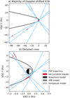 |
Fig. D.1 Location of possibly Doppler-shifted ion cyclotron waves, in the same format as Figure 9. |
| In the text | |
|
Fig. E.1 Number of elements per bin for the two interplanetary mag netic field configurations considered for Figure 10 of the main text. The conic bow shock model from Martinecz et al. (2009) is shown in black. |
| In the text | |
Current usage metrics show cumulative count of Article Views (full-text article views including HTML views, PDF and ePub downloads, according to the available data) and Abstracts Views on Vision4Press platform.
Data correspond to usage on the plateform after 2015. The current usage metrics is available 48-96 hours after online publication and is updated daily on week days.
Initial download of the metrics may take a while.