| Issue |
A&A
Volume 655, November 2021
|
|
|---|---|---|
| Article Number | A11 | |
| Number of page(s) | 25 | |
| Section | Cosmology (including clusters of galaxies) | |
| DOI | https://doi.org/10.1051/0004-6361/202141350 | |
| Published online | 28 October 2021 | |
Geometry versus growth
Internal consistency of the flat ΛCDM model with KiDS-1000
1
University of Oxford, Denys Wilkinson Building, Keble Road, Oxford OX1 3RH, UK
e-mail: This email address is being protected from spambots. You need JavaScript enabled to view it.
2
Department of Physics and Astronomy, University College London, Gower Street, London WC1E 6BT, UK
3
Institute for Astronomy, University of Edinburgh, Royal Observatory, Blackford Hill, Edinburgh EH9 3HJ, UK
4
Center for Theoretical Physics, Polish Academy of Sciences, Al. Lotników 32/46, 02-668 Warsaw, Poland
5
Ruhr University Bochum, Faculty of Physics and Astronomy, Astronomical Institute (AIRUB), German Centre for Cosmological Lensing, 44780 Bochum, Germany
6
Department of Astrophysical Sciences, Princeton University, 4 Ivy Lane, Princeton, NJ 08544, USA
7
Leiden Observatory, Leiden University, PO Box 9513, 2300 RA Leiden, The Netherlands
Received:
19
May
2021
Accepted:
3
September
2021
Abstract
We carry out a multi-probe self-consistency test of the flat Lambda Cold Dark Matter (ΛCDM) model with the aim of exploring potential causes of the reported tensions between high- and low-redshift cosmological observations. We divide the model into two theory regimes determined by the smooth background (geometry) and the evolution of matter density fluctuations (growth), each governed by an independent set of ΛCDM cosmological parameters. This extended model is constrained by a combination of weak gravitational lensing measurements from the Kilo-Degree Survey, galaxy clustering signatures extracted from Sloan Digital Sky Survey campaigns and the Six-Degree Field Galaxy Survey, and the angular baryon acoustic scale and the primordial scalar fluctuation power spectrum measured in Planck cosmic microwave background (CMB) data. For both the weak lensing data set individually and the combined probes, we find strong consistency between the geometry and growth parameters, as well as with the posterior of standard ΛCDM analysis. In the non-split analysis, for which one single set of parameters was used, tension in the amplitude of matter density fluctuations as measured by the parameter S8 persists at around 3σ, with a 1.5% constraint of S8 = 0.776−0.008+0.016 for the combined probes. We also observe a less significant preference (at least 2σ) for higher values of the Hubble constant, H0 = 70.5−1.5+0.7 km s−1 Mpc−1, as well as for lower values of the total matter density parameter Ωm = 0.289−0.005+0.007 compared to the full Planck analysis. Including the subset of the CMB information in the probe combination enhances these differences rather than alleviate them, which we link to the discrepancy between low and high multipoles in Planck data. Our geometry versus growth analysis does not yet yield clear signs regarding whether the origin of the discrepancies lies in ΛCDM structure growth or expansion history but holds promise as an insightful test for forthcoming, more powerful data.
Key words: cosmological parameters / methods: data analysis / cosmology: theory / large-scale structure of Universe / gravitational lensing: weak
© ESO 2021
1. Introduction
The dramatic increase in precision experienced by cosmology over the last 30 years has recently led to the discovery of potential inconsistencies in our cosmological model that previously might have been obscured by statistical errors. One of the most relevant of these inconsistencies is the apparent discrepancy between a subset of the free parameters of the concordance Λ cold dark matter (ΛCDM) model (Condon & Matthews 2018; Lahav & Liddle 2019) measured at early and late times of the Universe. The most notable manifestation of this tension is the 4.2σ (Riess et al. 2021) difference in the value of the Hubble constant, H0, between distance ladder estimates and the early-Universe cosmic microwave background (CMB) probe Planck (Planck Collaboration VI 2020). Moreover, late-Universe probes of the large-scale structure, such as weak gravitational lensing (WL) and galaxy clustering, prefer a lower amplitude of the growth of structure than Planck, with tension up to the 3.2σ level in the parameter  , where σ8 is the standard deviation of matter density fluctuations in spheres of radius 8 h−1 Mpc today and Ωm is the matter density parameter (Alsing et al. 2017; Joudaki et al. 2017; Loureiro et al. 2019; Asgari et al. 2021; Tröster et al. 2020; Kobayashi et al. 2020).
If confirmed, the reasons behind these discrepancies could be twofold. On the one hand, if we assume our cosmological theory to be correct, the origin of the tension must lie in the data or their analysis of either set of probes. On the other hand, if we decide to trust the current measurements, the tension would suggest a shortcoming of the theory used to analyse the data, such as new physics beyond the standard model (e.g. Mörtsell & Dhawan 2018; Capistrano et al. 2020; Abellan et al. 2020; Dainotti et al. 2021). Finally, one must also consider the possibility that both measurements and theory are correct and that the disagreement is solely due to statistical variance between the two sets of measurements.
Numerous efforts have been made to identify possible errors in the respective data analysis processes of each set of probes. Concerning the local measurements of the Hubble parameter, examples of these efforts can be found in the most recent review of the distance ladder (Riess et al. 2021). Large-scale structure surveys have also carried out extensive systematics checks and internal consistency tests; see Abbott et al. (2018a), Lemos et al. (2021) and Doux et al. (2021) for the Dark Energy Survey, Köhlinger et al. (2019), Wright et al. (2020), van den Busch et al. (2020), Giblin et al. (2021), Asgari et al. (2021) and Hildebrandt et al. (2021) for the Kilo-Degree Survey (KiDS), and Laurent et al. (2017) and Vargas-Magaña et al. (2018) for the Baryon Oscillation Spectroscopic Survey (BOSS) and the Extented Baryon Oscillation Spectroscopic Survey (eBOSS) respectively. As for the CMB probes, Efstathiou & Gratton (2021) undertook a thorough revision of the CamSpec Likelihood used to analyse Planck data in search of potential sytematics. Moreover, the initiative ‘Beyond Planck’ is currently conducting a thorough revision of the Planck and WMAP methodology (BeyondPlanck Collaboration 2020).
Recently, alternative calibrations of the cosmic distance ladder have shed doubts on the robustness of the Hubble tension (e.g. Freedman et al. 2019; Freedman 2021). Moreover, alternative methods of measuring the Hubble parameter locally seem to be in agreement with the CMB measurement rather than with the cosmic distance ladder (e.g. Abbott et al. 2018b; Hall 2021). However, no known systematic errors have convincingly explained the anomalously large value of H0 of the cosmic distance ladder yet (e.g. Freedman et al. 2019; Pesce et al. 2020). Similarly, the S8 tension has proven not to be relieved by combining data of independent late-Universe probes (e.g. Abbott et al. 2018a; Tröster et al. 2020; Heymans et al. 2021).
In this work we develop and apply methodology to test the self-consistency of the spatially flat ΛCDM model with the goal of providing guidance as to which regime of the theory could drive the observed tension. To do so, we differentiate between two theory regimes within the cosmological model: geometry; refereeing to the parts of the model related to the dynamics of the space-time and growth, concerning the formation of matter anisotropies on top of the dynamics of space-time. The key distinguishing factor between the two regimes is that geometry solely regards uniform background quantities while growth considers perturbations on this background. If the ΛCDM model is self-consistent, the same set of cosmological parameter values should correctly reproduce both of its theory regimes. We test this assumption by letting each theory regime be governed by an independent set of ΛCDM parameters. Then, we employ a range of high- and low-redshift cosmological probes to obtain constraints for each regime of the theory. Any discrepancies between the pairs of geometry and growth parameters would hint at the origin of potential failures in our current cosmological model. Moreover, the fact that this methodology studies background and perturbations independently allows us to more easily pinpoint the character and origin of the new physics behind the potential discrepancy.
Similar studies were conducted prior to this publication that also explore the effects of splitting certain parameters of a given cosmological model as a means to investigating its self-consistency. As early as 2004, Chu & Knox (2005) studied the consistency of the constraints coming from data on the ionisation history and on the pressure profile of the pre-recombination fluid in the context of flat ΛCDM by duplicating the baryon density parameter, Ωb, and allowing each instance to be constrained by one of the phenomena. In Abate & Lahav (2008) a similar exercise was performed on the total matter density parameter, Ωm, by having three instances, each controlled by a different physical observable in type Ia supernova (SN Ia) data. More recently, Ruiz & Huterer (2015) undertook a very similar analysis to the one presented in this work, with a similar selection and treatment of observables but limited to splitting Ωm. Beyond ΛCDM, Bernal et al. (2016) and Wang et al. (2007) undertook multi-probe studies of the consistency of the variable equation of state, cold dark matter (wCDM) model by splitting the equation-of-state parameter w, and the density parameter, ΩDE, of dark energy into their geometry and growth contributions.
During the final stages of our study, Muir et al. (2021) published a closely analogous investigation of geometry–growth consistency using several probes from the Dark Energy Survey in combination with external data. Our work is complementary in that it employs a different mix of data sources: WL data from KiDS-1000 (Asgari et al. 2021), galaxy clustering data from BOSS (Alam et al. 2017) and the 6 Degree Field Galaxy Survey (6dFGS; Beutler et al. 2011), Lyman-α and quasar clustering information from the Extended Baryon Oscillation Spectroscopic Survey (eBOSS; de Sainte Agathe et al. 2019; Blomqvist et al. 2019), and subsets of the Planck CMB temperature and polarisation anisotropy correlations. Moreover, our split is more comprehensive in that we duplicate the full flat-ΛCDM parameter space, whereas Ruiz & Huterer (2015) and Muir et al. (2021) limited themselves to a split in the dark matter density parameter only.
This work is structured as follows: In Sect. 2 we present the methodology of this work regarding the distinction between geometry and growth in the ΛCDM model and the resulting modelling of the observables of interest. In Sect. 3 we describe the data sets that we analyse. We discuss the likelihood analysis in Sect. 4 and present results in Sect. 5. In Sect. 6 we summarise our findings and conclude.
2. Methodology
2.1. Distinguishing geometry and growth
We adopted a classification of the theory of the ΛCDM model based on whether it keeps, or departs from a uniform background. Hence, any information regarding the formation of structure in the model can be traced to where it departs from a smooth background. Thus, we distinguished two theoretical regimes: on the one hand, a uniform background that describes the curvature and expansion history of the Universe, and on the other hand, a theory of perturbations that build up from the background and create the structures in the Universe1. We refer to these two regimes of the theory as geometry and growth, respectively.
In mathematical terms the departure from, or conservation of, such uniformity can be fully encapsulated in the choice of metric since its shape is fully determined by the assumptions that we make about the universe that we aim to describe. Furthermore, the fundamental role that the metric plays in Einstein gravity means that these assumptions propagate into the entirety of the theoretical predictions of the model. Of these predictions, we particularly focus on two: the field equations, that describe the relationship between matter and gravity, and the equations of motion of the stress-energy tensor fields, that describe how the content of the Universe evolves over time. The FLRW line element, that represents a uniform background, directly leads to the Friedmann field equations. Moreover, the Friedmann field equations can be combined into a conservation law for the field that describes its evolution. The perturbation of this uniform background metric ultimately leads to the Jeans equation, describing the evolution of matter density perturbations over cosmic time (e.g. Baker et al. 2014).
This dualistic understanding of the theory is extremely useful when calculating predictions of astrophysical phenomena. This is due to the fact that some phenomena can be accurately modelled purely within a particular regime. Thus, we can equivalently distinguish between geometry and growth observables as well as geometry and growth theory regimes. Furthermore, the modelling of more ‘complex’ observables might need a combination of background and perturbation physics.
Nonetheless, if the ΛCDM model is to be self-consistent, both regimes of the theory must be governed by the same set of parameters, and therefore, parameter constraints based on geometry observables should be consistent with those from growth ones. Similarly, observables whose modelling makes use of both theory regimes should exhibit internal consistency between the preferred parametrisations of their different calculation stages.
In this work we tested the self-consistency of the ΛCDM model by assigning to each theory regime its own set of cosmological parameters and simultaneously parametrising them using a set of geometry and growth observables. This allowed us to observe the parametrisation preferences of each regime such that potential discrepancies can be identified. From here on we denote the sets of parameters governing the geometry and growth regimes of the theory as pgeom and pgrow, respectively. In this analysis we sample over the following parameters: 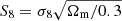 ; where σ8 is the root-mean-square of matter density fluctuations in spheres of 8 h−1 Mpc and Ωm is the total matter density parameter, the reduced Hubble parameter h = H0/(100 km s−1 Mpc−1), the reduced cosmological cold dark matter density ωcdm = Ωcdmh2, the reduced cosmological baryonic density ωb = Ωbh2 and the spectral index ns.
Simply splitting the parameter space into two subsets does not ensure independent constraints for the two theory regimes. This is because one can fully derive the growth aspects from the geometry parameters and vice versa, via the Jeans equation, in cosmological models in which gravitational collapse is quasistatic up to the linear level of the theory (Silvestri et al. 2013; Baker et al. 2014). An explicit demonstration of this duality in GR+ΛCDM can be found in Alam et al. (2009). Moreover, even if the set of geometry cosmological parameters cannot constrain parameters that explicitly relate to matter anisotropies (e.g. S8), fixing them would misrepresent this lack of constraining power. An analogous argument can be made for growth parameters that primarily affect the expansion history, such as h. We therefore assigned the same, uninformative priors to both parameter sets and vary the full set in each case.
There are alternative interpretations of the categories of geometry and growth and that the choice made in this work is not necessarily unique. For example, in Muir et al. (2021) growth is limited to describe only the late growth of structure based on the made argument that geometry and growth are analytically linked at the level of linear theory. These approaches are not contradictory but the different analysis choices prevent direct comparisons between the resulting constraints.
For the purposes of this work we limited ourselves to a spatially flat ΛCDM model. In agreement with Hildebrandt et al. (2020), we also assumed two massless neutrino species and a third massive species with mass mncdm = 0.06 eV/c2, as well as a temperature of the non-cold relic Tncdm = 0.71611 K.
2.2. Cosmological observables
In this section we introduce the physical observables used in this work, including a discussion of their geometry versus growth treatment; see Table 1 for an overview.
Geometry and growth classification of the observables used in our analysis.
2.2.1. Weak lensing
In general relativity mass induces in its surrounding space-time a non-Euclidean geometry. In agreement with Fermat’s principle, photons seek the path of least action through the curved space. These paths correspond to geodesic lines that are not straight in a Euclidean sense, thus causing light rays to appear bent. This deflection of light rays leads to similar observational effects as those of optical lenses, focusing and distorting the images we observe of celestial bodies that lie behind the lens. The effect of such lenses is usually quite weak, such that it can only be detected via statistical methods from large galaxy samples. This is referred to as weak lensing (WL).
Weak lensing measurements are an excellent tool to inspect the interplay between the different regimes of ΛCDM because it is sensitive to both geometry and growth. This is because the strength of the light deflection depends on the distances between the light source, the lens, and the observer, as well as the spatial distribution of the lenses and their density contrast with respect to the mean matter distribution. Formally, this duality can be observed in the key quantity of weak lensing, the lensing convergence κ (e.g. Bartelmann & Schneider 2001),
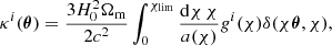 (1)
(1)
where we assume a spatially flat universe. Here, χ is the radial comoving distance, χlim is the radial comoving distance to the horizon, a is the scale factor, c is the speed of light in the vacuum, and θ is a two-dimensional vector that represents angular position on the sky. We also introduce the matter density contrast δ measured at a position and epoch determined by the comoving distance and the angular position. The lensing efficiency gi(χ) is defined as
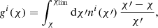 (2)
(2)
where ni(χ′) is the comoving distance distribution of source galaxies on which the lensing effect is measured, assigned to a tomographic redshift bin labelled by i. In practice, we measure the source distribution of redshifts, ni(z) = ni(χ) dχ/dz.
Since the effects of weak lensing are not strong enough to be directly observable, it is only possible to appreciate them statistically. The standard baseline two-point statistic to model weak lensing signals is the Fourier transform of the two-point correlation of the convergence across redshift bins i and j, the convergence power spectrum
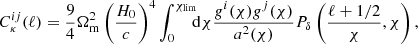 (3)
(3)
where Pδ(k, χ) is the (non-linear) matter power spectrum evaluated at wavenumber k and an epoch marked by χ. In Eq. (3) the Limber approximation was applied (Limber 1953).
Angular power spectra are not directly measurable from a restricted survey footprint. We employed band powers derived from angular correlation function measurements; see Joachimi et al. (2021), van Uitert et al. (2018), Schneider et al. (2002) for a detailed description. Band powers can be modelled as linear functionals of the angular convergence power spectra,
 (4)
(4)
for a band indexed by l, where the filter function  is given by Eq. (26) of Joachimi et al. (2021). The normalisation, 𝒩l, is defined such that the band powers trace ℓ2Cκ(ℓ) at the logarithmic centre of the bin, 𝒩l = ln(ℓup, l)−ln(ℓlo, l) with ℓup, l and ℓlo, l defining the edges of the top-hat band selection function for the bin indexed by l. Here, we have assumed that the model does not predict any B-modes, and we will only use the E-mode band powers in our analysis. This assumption is based on the work of Giblin et al. (2021) who showed that there is no significant detection of B-modes in KiDS-1000.
It is possible to classify the quantities that enter the convergence power spectrum as geometry- or growth-related. On the one hand, the cosmological dependence of the matter power spectrum Pδ is growth-related. On the other hand, the lensing efficiency solely concerns angular diameter distances (or comoving distances when assuming a flat universe), that are purely geometry-related. A more ambiguous decision is whether to consider the prefactor in Eq. (3) geometry or growth. This is due to the fact that, while these terms originate from the Poisson equation that relates the gravitational potential to its source, δ, in the context of the calculation of the observable they effectively act as a geometrical relationship that does not necessarily regard anisotropies. In agreement with the criteria of recent work (Muir et al. 2021), we consider these prefactors as geometry.
2.2.2. Baryon acoustic oscillations
Baryon acoustic oscillations (BAOs) cause enhanced matter overdensities at a characteristic physical separation scale that corresponds to the size of the sound horizon at the end of the drag epoch, rs(zd) (Peebles & Yu 1970; Hu & Dodelson 2002). The sound horizon is defined as the distance a pressure wave can travel from its time of emission in the very early Universe up to a given redshift. This can be expressed as
 (5)
(5)
where cs denotes the speed of sound, and where H(z) is the expansion rate at redshift z. The end of the drag epoch is defined as the time when photon pressure can no longer prevent gravitational instability in baryons around z ∼ 1020 (Komatsu et al. 2009). The redshift of this time is typically estimated using the following fitting formula:
![Mathematical equation: $$ \begin{aligned} z_{\rm d}= \frac{1291(\omega _{\rm m})^{0.251}}{1 + 0.659(\omega _{\rm m})^{0.828}} [1+ b_{1} (\omega _{\rm b})^{b_{2}}], \end{aligned} $$](/articles/aa/full_html/2021/11/aa41350-21/aa41350-21-eq13.gif) (6)
(6)
where b1 = 0.313(ωm)−0.419[1 + 0.607(ωm)0.674], b2 = 0.238(ωm)0.223 and ωm = ωcdm + ωb is the reduced cosmological matter density (see Komatsu et al. 2009).
Since the overdensity manifests anisotropically in redshift space as a three-dimensional shell, it is possible to measure the shift in the BAO peak position with respect to its position in a fiducial cosmology, parallel and perpendicular to the line of sight. Perpendicular to the line of sight, the BAO feature informs the trigonometric relationship
 (7)
(7)
where θ is the angle under which the scale of the sound horizon is observed, and DM(z) is the comoving angular diameter distance to redshift z, which in a flat universe is identical to the comoving radial distance χ(z). Parallel to the line of sight, the BAO feature allows us to measure the expansion history of the Universe. The BAO measurements along the line of sight can be use to constrain the relationship H(z)rs(zd).
We cast our BAO measurements in the form of the dimensionless ratios (Alam et al. 2017; du Mas des Bourboux et al. 2020; de Sainte Agathe et al. 2019; Blomqvist et al. 2019):
![Mathematical equation: $$ \begin{aligned} \alpha _\parallel = \frac{[D_{\rm H}/r_{\rm s}(z_{\rm d})]}{[D_{\rm H}/r_{\rm s}(z_{\rm d})]_{\rm fid}}; \quad \alpha _\perp = \frac{[\chi /r_{\rm s}(z_{\rm d})]}{[\chi /r_{\rm s}(z_{\rm d})]_{\rm fid}}, \end{aligned} $$](/articles/aa/full_html/2021/11/aa41350-21/aa41350-21-eq15.gif) (8)
(8)
to describe shifts perpendicular and parallel to the line of sight, where DH(z) = c/H(z) is the Hubble distance and the label ‘fid’ denotes a quantity evaluated at the aforementioned fiducial cosmology. Nonetheless, the quantities chosen to represent these parallel and perpendicular signatures of the BAO feature can vary from probe to probe.
It is also common to combine the perpendicular and parallel information in the volume-averaged angular diameter distance defined as
 (9)
(9)
or in the anisotropy parameter known as the Alcock-Paczynski parameter; FAP(z) (Alcock & Paczynski 1979), defined as:
 (10)
(10)
Although BAOs are a consequence of structure growth, their signature in the matter distribution can be translated into distance relationships that can be calculated without making use of density perturbations. This can be seen in the fact that, while the speed of propagation of BAOs, and thus the sound horizon, is a function of the matter content of the Universe, it can be completely calculated by assuming this content to be uniform. Therefore, measurements of the position of the BAO peak in the CMB or in the large-scale structure can be classified as pure geometry phenomena.
2.2.3. Redshift space distortions
Redshift space distortions (RSDs) are modifications to the clustering statistics of a given ensemble of objects due to their peculiar velocities along the line of sight on top of the recession velocity due to cosmological expansion (Kaiser 1987). RSDs are determined by peculiar motion in the gravitational potential of the surrounding matter distribution and thus governed by the Poisson equation, which makes them a pure growth effect. For galaxies on large, linear scales RSDs are dominated by the infall towards overdense structure, known as the Kaiser effect (Hamilton 1998).
Clustering two-point statistics as a function of transverse and line-of-sight separation can be used to extract RSDs via the quantity (e.g. Beutler et al. 2017)
 (11)
(11)
where f is the growth rate and δ is again the matter density contrast. Both f and σ8 are evaluated at the effective redshift of the measurement, as opposed to the use of σ8 in weak lensing that is always interpreted at z = 0.
2.2.4. Early-Universe geometry and growth parameters
The CMB is the richest source of cosmological information to date and particularly valuable as a complement to low-redshift probes of the large-scale structure. While a full re-analysis of Planck data is beyond the scope of this work, we would still like to make use of readily accessible CMB information that can be allocated cleanly to either the geometry or growth regimes. The primary CMB anisotropies can be described by a set of five cosmological parameters (Vonlanthen et al. 2010; Kosowsky et al. 2002): the reduced baryon density parameter ωb, the reduced cold dark matter density parameter ωcdm, the amplitude and spectral index of primordial scalar fluctuations, As and ns respectively, and the angle subtended by the sound horizon at end of recombination epoch θ* (cf. Eq. (7), evaluated at redshift z* ∼ 1100 as opposed to zd ∼ 1020). A detailed discussion of the role of each of these parameters in determining the physical properties of the CMB can be found in Mukhanov (2004).
The CMB information contained in the parameters ns and As is purely growth-related since they capture the primordial scalar fluctuation power spectrum
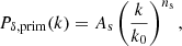 (12)
(12)
where k0 is the pivot scale of the power spectrum here set to the value of 0.05 Mpc−1 for consistency with Planck (Planck Collaboration VI 2020). In contrast, θ* is clearly a parameter solely concerned with the background cosmology as it relates the distance to the surface of last scattering to the size of the sound horizon.
The information contained in ωb and ωcdm cannot not readily categorised. On the one hand, they are informed by the relative height of the CMB peaks, related to density fluctuations, but also by the expansion history and the value of the speed of sound in the baryon-photon fluid, all describable in a smooth universe. Therefore we decided not to include CMB constraints on ωb and ωcdm in our analysis, but do make use of the marginalised posteriors of the combination {ns, As, θ*}, taking their correlation into account. We note that similar analyses (Muir et al. 2021) have employed the CMB shift parameter ℛ, a measure of the change of location of the first power spectrum peak with respect to a fiducial cosmology (Efstathiou & Bond 1999). While the ℛ parameter is a good alternative to constrain geometry, in this work we decided to use θ* as it is a direct analogue of quantities available for the large-scale structure BAO measurements. The ns constraint can be directly matched to the sampled ns values in our analysis to constrain growth. Similarly, As can be inferred from the sampled S8 value and matched to the CMB constraint to constrain growth. On the other hand, we treat θ* as another evaluation of the distance relationship in Eq. (7) and use it to constrain the geometry regime.
3. Data sets
To constrain the geometry and growth regimes of ΛCDM, we jointly analysed a range of recent measurements. A summary of the data sets employed in this work is given in Table 2.
Data sets used in our analysis, and their properties.
3.1. KiDS-1000 cosmic shear measurements
We employed cosmic shear measurements from the fourth data release of the European Southern Observatory’s Kilo Degree Survey (KiDS; Kuijken et al. 2019) incorporating data from the fully overlapping VISTA Kilo-Degree Infrared Galaxy Survey (VIKING; Edge et al. 2013). The KiDS and VIKING surveys were designed to be complementary and combine optical and near-infrared imaging in nine photometric bands (Wright et al. 2020). We analysed the now-public weak lensing shear catalogue dubbed KiDS-1000 from Giblin et al. (2021), which images 1006 deg2 on the sky2. This data set is divided into four photometric redshift bins of width Δz = 0.2 in the range 0.1 ≤ zB ≤ 0.9 and a fifth bin with 0.9 ≤ zB ≤ 1.2, based on their most probable Bayesian redshift zB inferred with the code BPZ (Benítez 2000). The redshift distributions of the five tomographic bins are then calibrated with deep spectroscopic samples that are reweighted using a self-organising map (Wright et al. 2020; Hildebrandt et al. 2021).
As summary statistic of the cosmic shear signal we adopted band power spectra estimated from the two-point correlation functions, which are analysed in Asgari et al. (2021). The corresponding KiDS-1000 cosmic shear likelihood is publicly available in the KiDS Cosmology Analysis Pipeline3 (KCAP) together with a MontePython interface4 that wraps the KCAP functionality. This likelihood requires two additional astrophysical nuisance parameters: the amplitude of intrinsic galaxy alignments AIA and the baryonic feedback parameter Abary; see Joachimi et al. (2021) for further details. Furthermore, five additional nuisance parameters δz allow for a shift of the mean of the redshift distribution in each tomographic bin within informative Gaussian prior set by the calibration procedure. Since these nuisance parameters do not have a cosmological interpretation we only kept one instance that was shared between the geometry and the growth instances of the cosmological code.
3.2. Galaxy clustering
The main data source we employed to draw constraints from the BAO and RSD observables were the Sloan Digital Sky Survey III (SDSS III; Eisenstein et al. 2011; Alam et al. 2017) and the Six-Degree Field Galaxy Survey (6dFGS) (Jones et al. 2009; Beutler et al. 2011). Concerning the first of the two surveys, we made use of the 12th data release of the galaxy clustering data set of the Baryon Oscillation Spectroscopic Survey (BOSS DR12) which forms part of SDSS III. BOSS DR12 contains records of 1.2 million galaxies over an area of 9329 deg2 and volume of 18.7 Gpc3, divided into three partially overlapping redshift slices centred at effective redshifts 0.38, 0.51, and 0.61.
We fitted the geometrical relations α∥ and α⊥ (Eq. (8)) as reported by the BOSS DR12 data products:
![Mathematical equation: $$ \begin{aligned} \frac{[H(z)]_{\rm fid}}{\alpha _\parallel } = \frac{H(z) [r_{\rm s}(z_{\rm d})]_{\rm fid}}{r_{\rm s}(z_{\rm d})}; \quad \alpha _\perp [\chi (z)]_{\rm fid} = \frac{\chi /r_{\rm s}(z_{\rm d})}{[r_{\rm s}(z_{\rm d})]_{\rm fid}}, \end{aligned} $$](/articles/aa/full_html/2021/11/aa41350-21/aa41350-21-eq22.gif) (13)
(13)
from the reconstruction of the BAO feature at the three different redshift bins where [rs(zd)]fid = 147.78 Mpc is the scale of the sound horizon at drag epoch as given by the fiducial cosmology used for the reconstruction. [H(z)]fid and [χ(z)]fid are the corresponding Hubble parameter and comoving radial distance for the fiducial cosmology, respectively. When fitting these distance relationships, rs(zd) was treated as a free quantity to be determined by the fitting process while [rs(zd)]fid was fixed to the value provided in the data products. Moreover, we fitted the three redshift measurements of fσ8(z) from RSD obtained using the anisotropic clustering of the pre-reconstruction density field (Alam et al. 2017). The BAO and RSD measurements of BOSS DR12 are two features extracted from the same set of observations. As such, they are not statistically independent. Thus, when analysing these two features, a combined analysis was performed mediated by the combined covariance matrix of the two sets of measurements from Alam et al. (2017). Moreover, we also accounted for the correlations present between the three BAO measurements with each other and between the three RSD measurements with each other resulting from the overlap in the used redshift bins.
This treatment of BOSS DR12 data given is different from Tröster et al. (2020) and Heymans et al. (2021), who performed a combined studies of KiDS with BOSS DR12 in a full-shape analysis. While performing a full-shape analysis in our study would increase the constraining power, it makes discerning between geometry and growth significantly more complex. Thus, we decided to trade constraining power for clarity in our proposed classification.
The 6dFGS is a combined redshift and peculiar velocity survey covering nearly the entire southern sky. The median redshift of the survey is z = 0.052. The 6dFGS BAO detection offers a constraint on the distance-redshift relation rs(zd)/Dv(zeff) at zeff = 0.106. Altogether, we employed a total of 10 data points from clustering surveys.
Both the SDSS and the 6dFGS overlap with KiDS in its northern and southern patches, respectively. While in principle this induces correlations with the weak lensing measurements, these are comfortably negligible, primarily because of the large survey areas outside the KiDS footprint used for clustering. Moreover, the measurements of α∥ and α⊥ tend to be extracted from larger physical scales than the weak lensing information. Joachimi et al. (2021) showed that cross-correlations between BOSS and KiDS are negligible even for a full-shape clustering analysis, and for the 6dFGS, which is at very low redshift, the correlation is even weaker.
3.3. Lyman-α forest and quasars
We employed high-redshift constraints on the BAO signature from SDSS-IV (Dawson et al. 2016) Data Release 14, observed as part of the eBOSS (Blanton et al. 2017). We did so by combining the auto- and cross-correlation analyses of three quasar samples from DR14Q (de Sainte Agathe et al. 2019; Blomqvist et al. 2019) which includes quasar clustering and Lyα forest absorption in the Lyα and Lyβ regions. The selected sample of tracer quasars contains 266 590 quasars in the range 1.77 < zq < 3.5. It includes 13 406 SDSS DR7 quasars Schneider et al. (2010) and 18 418 broad absorption line (BAL) quasars (Weymann et al. 1991). The Lyα sample is derived from a super set consisting of 194 166 quasars in the redshift range 2.05 < zq < 3.5, whereas the Lyβ sample is taken from a super set containing 76 650 quasars with 2.55 < zq < 3.5.
The BAO signal is detected both parallel and perpendicular to the line of sight in the auto-correlation of the two quasar samples as well as in the cross-correlation between the two. This allows for the measurement of the distance relationships α∥ and α⊥ described in Eq. (8), where the fiducial factors of normalisation are [DM/rs(zd)]fid = 39.26 and [DH/rs(zd)]fid = 8.581. As opposed to the rest of the data sets, when fitting the Lyα data we did not assume a Gaussian likelihood for the distance relationships. Instead, we interpolated the publicly available MCMC chains of the combined analysis of Lyα auto-correlation, quasar auto-correlation and Lyα-quasar cross-correlation5 from de Sainte Agathe et al. (2019), Blomqvist et al. (2019) and evaluated the two-dimensional interpolation function at the sampled α∥ and α⊥ to obtain the corresponding Δχ2-value relative to the best-fit χ2-value;  , obtained from Blomqvist et al. (2019, Table 5). When reporting the goodness of fit obtained using this likelihood, we employed the following formula
  ; where Δχ2 is the value inferred with our likelihood code and
  is the best goodness of fit found by Blomqvist et al. (2019). When combining these data sets, since goodness of fit values are additive, we simply added
  to the obtained Δχ2 of the combined data sets.
3.4. Cosmic microwave background anisotropies
We made use of the constraints resulting from the analysis of measurements of the cosmic microwave background (CMB) temperature and polarisation anisotropy maps of the European Space Agency’s satellite Planck (Planck Collaboration VI 2020) denoted as TT, TE, EE + Lowl + lowE and referred to in the following as ‘Planck 2018’. More specifically, we employed the posteriors on the cosmological parameters As and ns as two data points. Additionally, we adopted Planck’s posterior for the BAO angular scale  , where z* ∼ 1100 is the redshift of the end of the recombination epoch.
In order to convert the previously mentioned posteriors into data points, we employed the PYTHON Monte Carlo sample analysis package GETDIST (Lewis 2019) to first marginalise the public posterior chains of the Planck 2018 TT, TE, EE + Lowl + lowE set over all parameters except θ*, As and ns. Then, we extracted the best-fit values of the parameters by finding the maximum of the joint posterior probability density distribution function. Finally, we calculated the combined covariance matrix of the three parameters. In doing so, we approximated the marginalised posterior as a multivariate Gaussian, which is an accurate assumption (see e.g. Fig. A.3). This allowed us to associate an error bar with each data point and to evaluate the level of correlation between the three pseudo-measurements. This allowed us to build a Gaussian likelihood based on the three Planck constraints that we can use to inform our own parameter constraints. To distinguish this subset from the complete Planck posterior we label it as Recomb This methodology is analogous to that used by Muir et al. (2021) when extracting constraints from a MULTINEST chain of the TT + lowl Planck lite 2015 likelihood and to the θ* fitting process in Ruiz & Huterer (2015).
4. Likelihood analysis
Bayesian inference is employed to obtain constraints for the ΛCDM parameter sets governing the geometry and growth theory regimes: pgeom and pgrow, respectively. It relies on Bayes’ theorem to relate the probability of a given set of parameter values conditioned on the observed data D, known as the posterior probability P(pgrow, pgeom|D), to the probability of observing the data given a set of parameter values, known as the likelihood ℒ(D|pgrow, pgeom):
 (14)
(14)
Here, we also defined the prior Π for a set of model parameters and the evidence 𝒵(D), which is independent of the parameters.
In line with previous analyses, we chose a Gaussian likelihood for all data sets under consideration,
![Mathematical equation: $$ \begin{aligned}&\mathcal{L} (\boldsymbol{D}|\boldsymbol{p}_{\rm grow},\boldsymbol{p}_{\rm geom})\nonumber \\&\quad = \frac{\exp \{-\frac{1}{2}[\boldsymbol{D} - \boldsymbol{m}(\boldsymbol{p}_{\rm grow},\boldsymbol{p}_{\rm geom})]^TC^{-1}[\boldsymbol{D} -\boldsymbol{m}(\boldsymbol{p}_{\rm grow},\boldsymbol{p}_{\rm geom})]\}}{(2\pi )^\frac{N}{2} \sqrt{\det (C)}}\cdot \end{aligned} $$](/articles/aa/full_html/2021/11/aa41350-21/aa41350-21-eq29.gif) (15)
(15)
In this general expression, N is the dimension of the data vector, C is covariance matrix that describes the statistical uncertainty and the correlations between the elements of D, and m(pgeom, pgrow) is the vector composed of the model predictions for the observations measured in D, given the parameters. The weighted difference between the data and the model prediction is χ2-distributed for Gaussian data and will be used by us as a measure of the goodness of fit.
Bayesian inference takes into consideration the initial expectations for the values of the parameters prior to analysing the data via Π(p). The priors chosen in this work for the parameters in both sets pgeom and pgrow are the same as in the original KiDS-1000 analysis (Joachimi et al. 2021), which were shown to bare no effect on the S8 posteriors. We display the prior distributions in Table 3. We note that the KiDS cosmology priors are sufficiently conservative so as not to impact significantly on the posteriors of any of the probe combinations that we consider in this work. The table also provides a brief description of each parameter and specifies their role as either cosmological, nuisance or derived, i.e fully determined from the set of sampling parameters. We also show the treatment of each parameter as either split (i.e. present in both the geometry and the growth set of parameters) or shared (i.e. a single parameter was used to model both theory regimes).
Model parameters and their priors, adopted from Asgari et al. (2021).
The geometry and growth parametrisation entails a duplication of the cosmological parameter space and the associated prior volume, which affects model comparison and selection criteria (Handley & Lemos 2019a). We note that alternative choices of priors could prove useful in this regard. For instance, instead of the sets pgeom and pgrow one could employ their mean and difference as the sampling parameters. While the mean would be assigned the same set of priors as the traditional analysis, the prior on the parameter differences could more explicitly account for our expectations in deviations from ΛCDM. We will consider these options in future work.
The implementation of Bayesian inference relies on computer methods that make handling the typically high dimensionality of the parameter space feasible. This is especially true in this work where large parts of the parameter space have been doubled. In this work we made use of the cosmological parameter estimation code MONTEPYTHON 2COSMOS6 (Köhlinger et al. 2019), a modification of MONTEPYTHON (Audren et al. 2013; Brinckmann & Lesgourgues 2019) that allows us to sample duplicated instances of parameters simultaneously. MONTEPYTHON 2COSMOS achieves this by creating two separate instances of its underlying cosmological prediction code, CLASS (Blas et al. 2011; Lesgourgues 2011). Six pre-existing likelihoods from MONTEPYTHON were adapted into MONTEPYTHON 2COSMOS such that pgrow and pgeom can be assigned to the models of the observables discussed in Sect. 2.2; see Fig. 1 for a schematic overview. We employed the nested sampling algorithm MULTINEST (Feroz et al. 2009, 2019), which allows us to reliably explore the high-dimensional posterior.
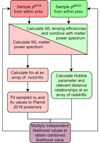 |
Fig. 1. Schematic of the complete MONTEPYTHON 2COSMOS pipeline developed for the purposes of this work. Two instances of the cosmological code, cosmology 1 and cosmology 2, independently sample the cosmological parameters for the two theory regimes, geometry and growth, respectively. These parameters are then passed to the likelihood modules to calculate the theoretical prediction for each individual probe. Finally, the respective independent likelihood values for each probe are multiplied to obtain the likelihood value of the combined data set. |
We assumed that the likelihoods for the different data sets employed are independent such that they can be combined by simple multiplication,  , where N is the number of probes used. The overlap region of the KiDS-1000 and BOSS footprints only accounts for 3% of the BOSS area, and hence it is safe to assume the two data sets are independent, as previous works have shown (Joachimi et al. 2021). Similarly, the BOSS and eBOSS data sets that we employed have been reported to be effectively independent (Ata et al. 2018). Also, the 6dfGS survey has been extensively used as an independent complement to SDSS data, as shown in Beutler et al. (2011).
The constraints of Planck 2018 are known to be in tension with those of KiDS-1000 in ΛCDM and therefore should not be combined per se. This tension has also been shown to persist even when the As value is fixed (see Tröster et al. 2021). However, the tension does not manifest in the subset of parameter constraints that we adopted from Planck (see Fig. A.3 for reference). While the Planck data points are independent of the low-redshift probes, joint posteriors employing this information will be necessarily correlated with full Planck constraints that we display alongside.
5. Results
In this section we present constraints on the geometry and growth cosmological parameters combining the weak lensing, clustering, Lyman-α, and Recomb data sets. When labelling the different results in tables and figures, results from the traditional, non-split analyses are simply labelled by the name of the combination of data sets employed, while labels of geometry and growth results also show the theory regime of the split model to which they belong. In Appendix A, we verify that these data sets are fully consistent with each other, and that our ‘traditional’ re-analysis of each data sets is consistent with the analyses presented in the literature. We also analyse the goodness of fit for each data combination finding that in all studied cases the models offer a good fit of the data. Moreover, we compare the traditional and geometry-growth split analysis, finding that while the split model is better at fitting the data, the improvement is not decisive at justifying the extra added degrees of freedom with respect the traditional analysis. We also calculate the Bayes factor and the deviance information criterion and find that none of the metrics display an statistically significant preference for either model for any combination of the data sets studied (see Appendix B for further details).
5.1. Geometry versus growth constraints
The marginalised posterior distributions for a subset of cosmological parameters, namely Ωm, σ8, and h, are illustrated in Fig. 2 for the split analysis of geometry (grey) and growth (green) as well as the traditional analysis with one single set of cosmological parameters (red). The leftmost row corresponds to an analysis of weak lensing data alone, while the rows to the right show the results obtained by subsequently adding the clustering, Lyman-α, and Recomb data sets. Additionally, we display the constraints from the Planck 2018 analysis (Planck Collaboration VI 2020) for reference in each panel (blue). The corresponding marginalised one-dimensional posteriors are shown in Fig. C.1 and the posteriors of the full set of cosmological parameters are presented in Appendix D.
 |
Fig. 2. Marginalised posterior distributions of σ8 and Ωm (top row), as well as h and Ωm (bottom row) for different combinations of data sets (columns). Each panel shows a superposition of four contours. Namely, the growth and geometry contours from the split analysis of the two theory regimes (green and grey contours respectively), the contour resulting from the traditional analysis with one set of cosmological parameters (red), and the reference contours from the Planck 2018 analysis (blue; Planck Collaboration VI 2020). |
We find that the constraining power on the geometry and growth theory regimes differs depending on the sensitivity of the probes with respect to the various cosmological parameter in the two theory regimes. For the parameters Ωm or ωcdm the constraining power of geometry and growth is comparable. Potential discrepancies in these parameters would thus be the most meaningful as both regimes are informed by the data. We also observe cosmological parameters for which only one theory regime has a significant constraining power. This is the case for S8, ns and σ8, that are only constrained by the growth regime. Consequently, the posteriors of their geometry counterparts are driven by the prior. Conversely, we find that h is overwhelmingly dominated by the geometry regime while its growth posterior is only weakly informed by the role of background quantities in the calculation of growth quantities. However, this contribution to the hgro parameter prevents it from simply returning its prior. Therefore, it is important to stress that while it is possible for the geometry regime to be uninformed about the perturbatory cosmological parameters, the growth theory regime necessarily holds information, even if very limited, on the background parameters since the perturbatory aspects of the theory are built from this background cosmology. Finally, we note that ωb is poorly constrained in both regimes with the data sets used.
The geometry and growth regimes explore independent directions of the parameter space, which results in posterior distributions of Ωm and σ8 that are orthogonal to each other. This was to be expected from the definition of each theory regime and the different information provided by geometry and growth observables. Figure 2 shows that this orthogonality significantly strengthens as more data sets are combined. A lack of correlation between pgeom and pgrow supports the meaningfulness of the geometry and growth categories as distinct theory regimes. The constraints on Ωm from growth and on σ8 from geometry are mainly dominated by the prior, except for the combination of weak lensing + clustering + Lyman-α + Recomb data, which puts stronger constraints from the growth regime on Ωm. This causes the two regimes to span over two independent directions in parameter space. While  is largely unconstrained, it is consistent with
  for all probe combinations, as detailed in Fig. 3. This finding deviates somewhat from the similar study by Muir et al. (2021) who found a 2σ preference for higher values of
  than
than  in their combined probe analysis. The numerical values for the obtained Ωm constraints for each of the studied combinations of data sets can be found in Table 4.
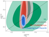 |
Fig. 3. Marginalised posterior for Ωm when comparing their geometry (horizontal axis) and growth (vertical axis) counterparts. We show the evolution of the contours as more data sources are added into the analysis. Namely, we display weak lensing (green), weak lensing combined with clustering data (grey), weak lensing combined with clustering and Lyman-α forest data (red) and finally weak lensing combined with clustering, Lyman-α forest and Recomb data (blue). |
Marginal Ωm constraints.
Overall, we observe minimal or little correlation between the different pairs of cosmological parameters for any of the studied combinations of data sets, finding all pairs of cosmological parameter to have a correlation coefficient below 0.2. The exception to this rule is the Ωm pair for which we observe a positive correlation of 0.48 between  when solely analysing weak lensing data, that is sensitive to both theory regimes. The correlation vanishes once additional data sources are included as these put stronger constraints on
  while leaving
  mostly unchanged.
The bottom row of Fig. 2 shows the marginalised posterior distributions for Ωm and h. The weak lensing observable by itself is not sensitive to the Hubble parameter, which is why the posterior distributions for h are prior-dominated for both geometry and growth, as well as for the traditional analysis. By adding additional data sets to the analysis, the geometry constraints shrink while the growth ones remain significantly wider, narrowing towards a Ωmh = const degeneracy constrained by the peak position of the matter power spectrum.
Comparing the posterior resulting from the traditional analysis to the ones obtained in the split analysis of the two theory regimes in the top row of Fig. 2, we find that, as was expected, the traditional contours reside at the intersection between the geometry and growth contours. While the constraints on Ωm and σ8 from geometry and growth by themselves are quite weak, the combination of the two regimes results in the ‘banana-shaped’ contour, which is most noticeable in the leftmost panel showing the constraints obtained from solely analysing weak lensing data. The good agreement between the two theory regimes internally and the traditional constraints is also evidenced by the negligible change in the goodness of fit (see Table B.1). However, tension with the full Planck analysis remains throughout, which we will discuss further in Sect. 5.2.
We quantify the level of consistency between the two theory regimes by considering the posterior distribution of the difference between the parameter duplicates, which is shown in Fig. 4 for three selected cosmological parameters: S8, Ωm, and h. Visually, the marginalised posterior distributions show good agreement with the zero point. This indicates no tension between parameters in the two theory regimes. We quantify the tension between parameter duplicates following the methodology of Köhlinger et al. (2019). We find good agreement between theory regimes for all combinations of parameters with a maximum offset of 1.27σ which is observed in the posterior distribution of Δh and ΔΩm for weak lensing + clustering data.
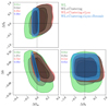 |
Fig. 4. Marginalised posterior distributions of the difference between geometry and growth parameter duplicates of S8, Ωm, and h. Each panel shows the contours for the combinations of data sets WL (green), WL + Clustering (black), WL + Clustering + Lyα (red) and WL + Clustering + Lyα + Recomb (blue). At the top-left corner of each panel we display the σ-level tension of each contour with respect to the null value pgrow = pgeom for all combination of data sets. |
Finally, we do not observe any new correlations between the different instances of the cosmological parameters and the nuisance parameters beyond those present in the traditional analysis. In particular, we do not see a correlation between the growth instance of Ωm and the nuisance parameter AIA as reported for weak lensing data by Muir et al. (2021). However, it must be noted that this finding may be influenced by the fact that DESY1 and KiDS-1000 model the impact of intrinsic alignments differently.
5.2. Tension with full Planck data
The presence of tension between our analyses and the full Planck contours suggests that its cause may lie in the weak lensing observable, common to all cases of study, or in the ΛCDM model. The most recent cosmic shear analysis of KiDS-1000 (Asgari et al. 2021) found a 3σ disagreement in their estimate of the cosmological parameter S8 with respect to the prediction of the Planck 2018 analysis of the CMB. This tension has been shown to persist both when combining the KiDS-1000 data with other probes (Heymans et al. 2021) and when considering extensions of the ΛCDM model (Tröster et al. 2021).
The level of consistency between BOSS DR12 data on galaxy clustering (Alam et al. 2017) and Planck 2018 depends on the chosen method of data compression (Sánchez et al. 2017; Loureiro et al. 2019; Kobayashi et al. 2020). Tröster et al. (2020) showed that when employing the geometrical quantities α⊥ and α∥ the data are not in tension with the ΛCDM parameters of Planck 2018. When cast into ΛCDM, the full shape analysis BOSS DR12 prefers a lower value of σ8 than Planck 2018 at 2.1σ. However, when the tension is computed for the whole parameter space using the suspiciousness statistic (Handley & Lemos 2019a), the two probes are in good agreement. The same considerations have to be made when assessing the consistency of the eBOSS DR14 data set with other surveys. In the α⊥ and α∥ framework, the eBOSS DR14 has been shown to be consistent with the Planck 2016 (Planck Collaboration XIII 2016) best-fit flat ΛCDM model, with a mild deviation of 1.7σ (Blomqvist et al. 2019). However, a non-negligible degree of discrepancy; between 2 and 2.5σ, has been reported when constraints are cast into the ΛCDM framework (Aubourg et al. 2015; Addison et al. 2018).
Finally, our implementation of the CMB data directly uses Planck 2018 posteriors as data points ensuring a perfect agreement with the early-Universe probe. Interestingly, the analysis of Recomb data is in good agreement with that of WL (see Fig. A.3), suggesting that the cause of the tension between Planck 2018 and WL must be driven by the features in the Planck data over which we marginalise to create the Recomb data set.
Thus, of the four data sets considered in this work, only KiDS-1000 is in significant tension with Planck 2018. This is simply a consequence of the tension manifesting in the amplitude of structure growth for which the weak lensing data are most constraining. Nonetheless, this does not exclude the possibility of new tensions appearing upon the combination of data sets which independently are in good agreement with Planck 2018; see the discussion for Ωm and h below.
Since we use KiDS-1000 as our base observable in all combinations of data sets, we observe that the tension on S8 carries on to all our combinations of data sets. While the tension can already be appreciated in Figs. 2 and C.1, we highlight this disagreement in Fig. 5, which shows the constraints on the parameter S8 for all the studied combinations of data sets, and for the traditional and growth parameters (the geometry constraints default to the prior and are not shown). We also show the maximum posterior (MAP) values for S8 and the associated 68% credible interval (CI) calculated using its projected joint highest posterior density PJ-HPD (see Joachimi et al. 2021 for reference) in Table 5. The MAP values are directly inferred from the posterior distribution of sampling parameters. However, the limited number of samples in the posterior chains leads to some scatter in the MAP values, which is noticeable for the broader posterior in the weak lensing-only case. Therefore, we infer the MAP values for this specific data set using the Nelder-Mead optimisation method (Nelder & Mead 1965; see Joachimi et al. 2021 for details).
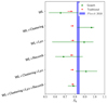 |
Fig. 5. S8 best-fit parameter values with their associated 1σ confidence regions obtained from the different combinations of data sets explored in this work. In top to bottom order we display the data sets WL, WL + Clustering, WL + Lyα, WL + Recomb, WL + Clustering + Lyα and finally WL + Clustering + Lyα + Recomb. The numerical value of the quantities displayed can be found in Table 5. |
Marginal S8 constraints.
We explicitly quantify this tension under the assumption of Gaussian and independent marginal posteriors. In this case the tension τ between two data sets i and j for a parameter p is given by
![Mathematical equation: $$ \begin{aligned} \tau _{ij} = \frac{|\overline{p}_{i} - \overline{p}_{j}|}{\sqrt{\mathrm{Var}[p_{i}]+\mathrm{Var}[p_{j}]}}, \end{aligned} $$](/articles/aa/full_html/2021/11/aa41350-21/aa41350-21-eq66.gif) (16)
(16)
where the barred quantities refer to the mean values of the distributions and Var to their variance. We provide the obtained values of the tension between the traditional analyses of the different combinations of data sets with Planck 2018 for the parameter S8 in Table 6. We see that the tension between the traditional and Planck 2018 S8 posterior distributions stays within 2 to 3σ for all combinations of data sets.
Level of tension between traditional analysis and Planck for the parameters S8 and Ωm.
Since each theory regime subset of parameters in our split model is a full ΛCDM model, it is possible to obtain the level of tension between geometry and growth with Planck 2018. The growth constraints are much weaker and hence not in tension although the combined constraint prefers a lower S8 value than Planck. We observe a slightly lower tension in S8 between our traditional KiDS-1000 only and Planck 2018 than Asgari et al. (2021) who employed a different summary statistic (COSEBIs) for their tension assessment. It is important to note that no particular choice of summary statistics is more powerful or more discrepant. Instead, the variance in the reported tension value for each summary statistic is due to slight differences in the degeneracy direction between the statistics which the parameter S8 does not perfectly capture. Moreover, our mean estimate is obtained directly from the posterior chains sampled with MULTINEST, that is less accurate than the Nelder-Mead optimisation of Asgari et al. (2021).
It is remarkable that the level of tension between traditional and Planck contours increases by 0.3σ when our Recomb data (i.e. the acoustic peak angular scale and the primordial power spectrum parameters) is included in the analysis. From Table 5, it is possible to see Clustering and Lyman-α data push the S8 constraints towards higher values more affine to the full Planck result, whereas Recomb; a subset of the CMB data, has the opposite effect, which may seem counter-intuitive. However, we argue that this trend can be understood as a manifestation of the high versus low multipole discrepancy within Planck (see Fig. 21 of Planck Collaboration VI 2020). Despite being a subset of the Planck 2018 TTTEEE constraints for which there is no low versus high multipole discrepancy, Recomb is largely informed by the TT anisotropies within multipoles ℓ < 800, and the low-ℓ TT Planck posterior is in excellent agreement with our joint probe analysis. Thus, it is possible to see how the combination of the Lyα data set preference for low values of Ωm in addition to the orthogonality between the degeneracy directions of the WL and Recomb contours increases the combined analysis tension. In Fig. 6 an illustration of the Lyα data set preference for low values of Ωm (left panel) and the orthogonality between the degeneracy directions of the WL and Recomb contours (right panel) is shown.
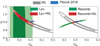 |
Fig. 6. Two-dimensional constraints for the combination of parameters Ωm − σ8 of the traditional analyses of Lyα+WL data (left) and of Recomb+WL (right). In both panels the empty black contours are the WL alone constraints while the filled blue ones are the Planck contours. Left panel: green contours show the Lyα constraints while the red contours show their combination with WL. Similarly, in the right panel: green contours show the Recomb constraints while the red contours show their combination with WL. The full posterior of these analyses can be seen in Figs. A.2 and A.3 respectively. |
In contrast, the tentative signs of tension with the full Planck constraints manifest not only in S8 or σ8, but extend to Ωm and h; as seen in Fig. 2. Discrepancy levels for Ωm are also given in Table 6 and reach 2.8σ for the joint probe analysis including Recomb data and 2.4σ in the WL + Clustering + Lyα + Recomb case. The Lyman-α forest data also has a preference for a somewhat lower Ωm than full Planck, which translates into a 2.3σ discrepancy. While the non-Gaussian shape of the marginal posterior for h prevents us from applying Eq. (16) more generally, in the WL + Clustering + Lyα + Recomb case the contours are sufficiently close to normal to apply the tension estimator, yielding a 2.0σ tension in h. In agreement with the low-ℓ Planck posterior, our joint probe posterior prefers lower values of Ωm and higher values of h than full Planck, with MAP values of 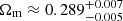 and
and 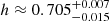 .
.
It is important to bear in mind that our joint probe analysis including the Recomb data is not statistically independent from the full Planck 2018 constraints, violating the assumption made to obtain Eq. (16). We leave a quantification of the level of correlation to future work. In principle, this correlation could lower or increase tension, dependent on the parameter degeneracies in the complement of the Planck data that we did not employ in our analysis. However, since the Planck high-ℓ constraints display the same degeneracy directions for the key parameters Ωm, σ8, and h as the low-ℓ subset, it is reasonable to assume that this correlation is positive, and hence our tension estimates of Table 5 are lower bounds on the true level of discrepancy.
6. Conclusions
In this work we developed a multi-probe self-consistency test of the spatially flat ΛCDM model with the aim of exploring potential causes of the cosmic tension within the current cosmological theory. In order to do so, we divided our model into two theory regimes, geometry and growth, distinguishing between the strictly uniform background and the formation of matter density fluctuations on top of this background, respectively. Making use of this distinction, we classified a series of cosmological observables, or parts thereof, as geometry or growth depending on the theory regime needed to model them within the ΛCDM model. We duplicated the ΛCDM parameter space into two independent copies, pgrow and pgeom, and let each govern its respective set of observables.
As cosmological observables, we employed weak lensing (WL) cosmic shear measurements from the latest data release of the Kilo Degree Survey (KiDS-1000), and measurements of the galaxy and Lyman-α (Lyα) BAO feature distance relationship from the 12th data release of the Baryon Oscillation Spectroscopic Survey (BOSS DR12), as well as from the 14th data release (DR14) of the eBOSS and the 6 Degree Field Galaxy Survey (6dFGS). We also used growth rate measurements from BOSS DR12. Moreover, we made use of the Planck 2018 posterior distributions for the cosmological parameters As and ns and the angular scale of the sound horizon θ* as pseudo-data points. We grouped these observables into four data sets: WL composed of the KiDS-1000 data, clustering which combined BOSS DR12 and the 6dfGS galaxy clustering measurements, Lyα composed of eBOSS DR14 data, and Recomb, containing the subset of the Planck 2018 posterior. Constraints for pgrow and pgeom were obtained using a modified version of the Bayesian parameter estimation code MONTEPYTHON 2COSMOS. In order to explore the extended parameter space we made use of Monte Carlo Markov chains while employing the nested sampler MULTINEST. The code developed to perform this analysis is made publicly available7.
We generally found very good agreement between all probes considered, including a subset of CMB data we used, with little variation in the goodness of fit. The geometry and growth parameters are consistent throughout, and the additional degrees of freedom in the model due to the split are not preferred by the data. The constraints on pgrow and pgeom converge towards the those found by the traditional ΛCDM analysis that does not duplicate parameters for all the studied combinations of data sets. We also observed that pgrow and pgeom explore different directions of the parameter space, their contours tending to be orthogonal to each other. Thus, we conclude that our constraints on pgrow and pgeom support the geometry versus growth distinction as a meaningful classification of the ΛCDM model.
Regarding the S8 parameter tension between low- and high-redshift probes, our analysis produced tension levels between 2 and 3σ for the traditional constraints of different probe combinations and Planck 2018 (Planck Collaboration VI 2020). The joint probe growth constraint on S8 also prefers lower values, but is not in tension due to substantially larger statistical errors. The traditional constraints of the parameters Ωm and h also reach discrepancies in the 2 and 3σ range, with larger values preferred for h and smaller values preferred for Ωm, in particular when our subset of CMB data is included. As this subset is primarily informed by large angular scales in the Recomb, this result supports earlier indications that the cosmic tensions in S8, and possibly also H0, are driven by multipoles ℓ > 800 in Planck (Addison et al. 2016; Planck Collaboration VI 2020).
In comparison to the recent similar analysis by Muir et al. (2021), our work employs an alternative distinction between geometry and growth solely based on the need to consider matter anisotropies in the modelling of the cosmological observable, irrespective of whether the matter anisotropies reside in the present or early Universe. This leads to a different classification of cosmological observables between the two works. Nonetheless, both Muir et al. (2021) and this work report an excellent degree of agreement between the two considered regimes. However, we do not observe the slight preference for higher values of  as seen by Muir et al. (2021), nor do we find any significant correlations between
  and the shared nuisance parameter for the intrinsic alignment amplitude, AIA.
To conclude we outline possible avenues for improvements that future iterations of the methodology presented in this work could consider. On the theoretical side, it would be interesting to study the feasibility of geometry versus growth splits beyond ΛCDM. It is clear that the distinction proposed in this work can be extrapolated straightforwardly to modified models that only introduce changes to the background cosmology, such as non-flat ΛCDM models or dark energy models with an effective equation of state, which have proven to be successful at encapsulating a wide variety of models (Traykova et al. 2021; García-García et al. 2020). Another type of modification that is compatible with this framework is a time-varying Newton’s constant for gravity because it does not change the shape of the Jeans equation (Baker et al. 2014). Other, more involved modifications could include scale-dependent modifications to the growth of structure. More general parametrisations than a simple duplication of ΛCDM parameters would have to be considered, and the link between the background and the growth of structure, via the Jeans equation and its non-linear corrections, carefully investigated.
The geometry and growth split is complementary to other empirical extensions to the standard ΛCDM model, such as μ − Σ models (Pogosian & Silvestri 2016). Theses models test for the consistency of the predictions of general relativity for relativistic and non-relativistic matter, whereas our split analysis explores the consistency between the predictions for the expansion history and structure growth. As opposed to previous works that subdivided the ΛCDM parameter space between geometry and growth, in this work we fully duplicated the parameter space; assigning one complete set of ΛCDM parameters to each theory regime. This was done with the aim of ensuring the independence of the constraints of each theory regime and of adequately capturing the uncertainty induced by the limited information available to each regime. Reflecting on this choice of analysis, geometry’s complete lack of constraining power on parameters that exclusively regards the anisotropies in the matter density field relegates the geometry instances of such parameters as simple measures of uncertainty. Therefore, future analyses could avoid sampling over said parameters in the geometry regime and use the assigned prior distributions as the measures of uncertainty when deriving quantities of interest.
Future applications should strive to incorporate new measurements on similar or different physical observables that could be added as new sources of constraining power. Specially, efforts should be directed towards performing a full-shape analysis of the LSS matter power spectrum as shown in Tröster et al. (2020) and Heymans et al. (2021) instead of the BAO and RSD feature analysis used in this work. Similarly, the current treatment of CMB data should be replaced by a more rigorous geometry and growth analysis of the full CMB data set, complemented by an analogous split of the CMB lensing likelihood (Planck Collaboration VIII 2020) observable equivalent to the one undertaken for KiDS-1000.
In addition to this, we recommend updating the galaxy clustering data to the latest eBOSS DR16 release (Alam et al. 2021), which also includes σ8 at high redshifts from quasar density measurements as well as high-redshift galaxy measurements (Zhao et al. 2021). Particularly adding to the currently weaker growth constraints, future works could consider studying the addition of Sunyaev-Zeldovich measurements of cluster counts (Planck Collaboration XXIV 2016), as well as the Integrated Sachs-Wolfe effect (Planck Collaboration XXI 2016; Stölzner et al. 2018). The geometry versus growth approach holds promise to yield novel insights with the powerful data from forthcoming surveys, including DESI8 (DESI Collaboration 2016), Euclid9 (Laureijs et al. 2011), and the LSST at the Rubin Observatory10 (The LSST Dark Energy Science Collaboration 2018).
As in standard structure formation theory, we assumed here that structure growth does not feed back significantly on the expansion history; see Clarkson et al. (2011) for a detailed discussion about this backreaction.
This assessment is subject to the nested sampler accuracy in the calculations of the evidence. In order to assure a reliable calculation of the evidence the following settings for MULTINEST were used: NS_max_iter: 10000000, NS_importance_nested_sampling: True, NS_sampling_efficiency: 0.3, NS_n_live_points: 1000, NS_evidence_tolerance: 0.1.
Acknowledgments
We thank Carlos Garcia-Garcia, David Alonso, and Shahab Joudaki for useful discussions. JRZ is supported by an STFC doctoral studentship and a Royal Astronomical Society summer student bursary. BS and BJ acknowledge support by the UCL Cosmoparticle Initiative. MA, BG, CH, and TT acknowledge support from the European Research Council under grant number 647112. MB is supported by the Polish National Science Center through grants no. 2020/38/E/ST9/00395, 2018/30/E/ST9/00698 and 2018/31/G/ST9/03388, and by the Polish Ministry of Science and Higher Education through grant DIR/WK/2018/12. AD, HH, JLvdB, and AHW are supported by an European Research Council Consolidator Grant (No. 770935). BG also acknowledges support from the Royal Society through an Enhancement Award (RGF/EA/181006). CH also acknowledges support from the Alexander von Humboldt Foundation in the framework of the Max Planck-Humboldt Research Award endowed by the Federal Ministry of Education and Research. HH is also supported by a Heisenberg grant of the Deutsche Forschungsgemeinschaft (Hi 1495/5-1). KK acknowledges support from the Royal Society and Imperial College. TT also acknowledges funding from the European Union’s Horizon 2020 research and innovation programme under the Marie Skłodowska-Curie grant agreement No. 797794. The analysis made use of the software tools SCIPY (Virtanen et al. 2020), NUMPY (Harris et al. 2020), MATPLOTLIB (Harris et al. 2020), CLASS (Lesgourgues 2011), GetDist (Lewis 2019), MULTINEST (Feroz et al. 2009, 2019), MONTEPYTHON (Brinckmann & Lesgourgues 2019; Audren et al. 2013) and MONTEPYTHON 2COSMOS (Köhlinger et al. 2019). Based on observations made with ESO Telescopes at the La Silla Paranal Observatory under programme IDs 177.A-3016, 177.A-3017, 177.A-3018, 179.A-2004, 298.A-5015, and on data products produced by the KiDS consortium. Based on observations obtained with Planck (http://www.esa.int/Planck), an ESA science mission with instruments and contributions directly funded by ESA Member States, NASA, and Canada. We acknowledge the efforts of the staff of the Anglo-Australian Observatory, who have undertaken the observations and developed the 6dF instrument. Funding for the Sloan Digital Sky Survey IV has been provided by the Alfred P. Sloan Foundation, the US Department of Energy Office of Science, and the Participating Institutions. SDSS-IV acknowledges support and resources from the Center for High Performance Computing at the University of Utah. The SDSS website can be found at www.sdss.org. SDSS-IV is managed by the Astrophysical Research Consortium for the Participating Institutions of the SDSS Collaboration including the Brazilian Participation Group, the Carnegie Institution for Science, Carnegie Mellon University, Center for Astrophysics, Harvard & Smithsonian, the Chilean Participation, the French Participation Group, Instituto de Astrofísica de Canarias, The Johns Hopkins University, Kavli Institute for the Physics and Mathematics of the Universe (IPMU)/University of Tokyo, the Korean Participation Group, Lawrence Berkeley National Laboratory, Leibniz Institut für Astrophysik Potsdam (AIP), Max-Planck-Institut für Astronomie (MPIA Heidelberg), Max-Planck-Institut für Astrophysik (MPA Garching), Max-Planck-Institut für Extraterrestrische Physik (MPE), National Astronomical Observatories of China, New Mexico State University, New York University, University of Notre Dame, Observatário Nacional/MCTI, The Ohio State University, Pennsylvania State University, Shanghai Astronomical Observatory, United Kingdom Participation Group, Universidad Nacional Autónoma de México, University of Arizona, University of Colorado Boulder, University of Oxford, University of Portsmouth, University of Utah, University of Virginia, University of Washington, University of Wisconsin, Vanderbilt University, and Yale University. Author contributions: All authors contributed to the development and writing of this paper. The authorship list is given in two groups: the lead authors (JRZ, BS, BJ), followed by an alphabetical group of co-authors who have either made a significant contribution to the data products or to the scientific analysis.
References
- Abate, A., & Lahav, O. 2008, MNRAS, 389, L47 [NASA ADS] [CrossRef] [Google Scholar]
- Abbott, T. M. C., Abdalla, F. B., Alarcon, A., et al. 2018a, Phys. Rev. D, 98, 043526 [NASA ADS] [CrossRef] [Google Scholar]
- Abbott, T. M. C., Abdalla, F. B., Annis, J., et al. 2018b, MNRAS, 480, 3879 [Google Scholar]
- Abellan, G. F., Murgia, R., Poulin, V., & Lavalle, J. 2020, ArXiv e-prints [arXiv:2008.09615] [Google Scholar]
- Addison, G. E., Huang, Y., Watts, D. J., et al. 2016, ApJ, 818, 132 [CrossRef] [Google Scholar]
- Addison, G. E., Watts, D. J., Bennett, C. L., et al. 2018, ApJ, 853, 119 [Google Scholar]
- Alam, U., Sahni, V., & Starobinsky, A. A. 2009, ApJ, 704, 1086 [NASA ADS] [CrossRef] [Google Scholar]
- Alam, S., Ata, M., Bailey, S., et al. 2017, MNRAS, 470, 2617 [Google Scholar]
- Alam, S., Aubert, M., Avila, S., et al. 2021, Phys. Rev. D, 103, 083533 [NASA ADS] [CrossRef] [Google Scholar]
- Alcock, C., & Paczynski, B. 1979, Nature, 281, 358 [NASA ADS] [CrossRef] [Google Scholar]
- Alsing, J., Heavens, A., & Jaffe, A. H. 2017, MNRAS, 466, 3272 [Google Scholar]
- Andrae, R., Schulze-Hartung, T., & Melchior, P. 2010, ArXiv e-prints [arXiv:1012.3754] [Google Scholar]
- Asgari, M., Lin, C.-A., Joachimi, B., et al. 2021, A&A, 645, A104 [NASA ADS] [CrossRef] [EDP Sciences] [Google Scholar]
- Ata, M., Baumgarten, F., Bautista, J., et al. 2018, MNRAS, 473, 4773 [NASA ADS] [CrossRef] [Google Scholar]
- Aubourg, É., Bailey, S., Bautista, J. E., et al. 2015, Phys. Rev. D, 92, 123516 [Google Scholar]
- Audren, B., Lesgourgues, J., Benabed, K., & Prunet, S. 2013, JCAP, 1302, 001 [Google Scholar]
- Baker, T., Ferreira, P., & Skordis, C. 2014, Phys. Rev. D, 89, 024026 [NASA ADS] [CrossRef] [Google Scholar]
- Bartelmann, M., & Schneider, P. 2001, Phys. Rep., 340, 291 [Google Scholar]
- Benítez, N. 2000, ApJ, 536, 571 [Google Scholar]
- Bernal, J. L., Verde, L., & Cuesta, A. J. 2016, JCAP, 2016, 059 [CrossRef] [Google Scholar]
- Beutler, F., Blake, C., Colless, M., et al. 2011, MNRAS, 416, 3017 [NASA ADS] [CrossRef] [Google Scholar]
- Beutler, F., Seo, H.-J., Saito, S., et al. 2017, MNRAS, 466, 2242 [Google Scholar]
- BeyondPlanck Collaboration (Andersen, K. J., et al.) 2020, ArXiv e-prints [arXiv:2011.05609] [Google Scholar]
- Blanton, M. R., Bershady, M. A., Abolfathi, B., et al. 2017, AJ, 154, 28 [Google Scholar]
- Blas, D., Lesgourgues, J., & Tram, T. 2011, JCAP, 2011, 034 [Google Scholar]
- Blomqvist, M., du Mas des Bourboux, H., Busca, N. G., et al. 2019, A&A, 629, A86 [NASA ADS] [CrossRef] [EDP Sciences] [Google Scholar]
- Brinckmann, T., & Lesgourgues, J. 2019, Phys. Dark Univ., 24, 100260 [Google Scholar]
- Capistrano, A. J. S., Cabral, L. A., Marão, J. A. P. F., & Coimbra-Araújo, C. H. 2020, ArXiv e-prints [arXiv:2009.02167] [Google Scholar]
- Chu, M., & Knox, L. 2005, ApJ, 620, 1 [NASA ADS] [CrossRef] [Google Scholar]
- Clarkson, C., Ellis, G., Larena, J., & Umeh, O. 2011, Rept. Prog. Phys., 74, 112901 [NASA ADS] [CrossRef] [Google Scholar]
- Condon, J. J., & Matthews, A. M. 2018, PASP, 130, 073001 [NASA ADS] [CrossRef] [Google Scholar]
- Cuceu, A., Farr, J., Lemos, P., & Font-Ribera, A. 2019, JCAP, 2019, 044 [Google Scholar]
- Dainotti, M. G., De Simone, B., Schiavone, T., et al. 2021, ApJ, 912, 150 [NASA ADS] [CrossRef] [Google Scholar]
- Dawson, K. S., Kneib, J.-P., Percival, W. J., et al. 2016, AJ, 151, 44 [Google Scholar]
- de Sainte Agathe, V., Balland, C., du Mas des Bourboux, H., et al. 2019, A&A, 629, A85 [NASA ADS] [CrossRef] [EDP Sciences] [Google Scholar]
- DESI Collaboration (Aghamousa, A., et al.) 2016, ArXiv e-prints [arXiv:1611.00036] [Google Scholar]
- Doux, C., Baxter, E., Lemos, P., et al. 2021, MNRAS, 503, 2688 [NASA ADS] [CrossRef] [Google Scholar]
- du Mas des Bourboux, H., Rich, J., Font-Ribera, A., et al. 2020, ApJ, 901, 153 [CrossRef] [Google Scholar]
- Edge, A., Sutherland, W., Kuijken, K., et al. 2013, The Messenger, 154, 32 [NASA ADS] [Google Scholar]
- Efstathiou, G., & Bond, J. R. 1999, MNRAS, 304, 75 [NASA ADS] [CrossRef] [Google Scholar]
- Efstathiou, G., & Gratton, S. 2021, Open J. Astrophys., 4, 8 [CrossRef] [Google Scholar]
- Eisenstein, D. J., Weinberg, D. H., Agol, E., et al. 2011, AJ, 142, 72 [Google Scholar]
- Feroz, F., Hobson, M. P., & Bridges, M. 2009, MNRAS, 398, 1601 [NASA ADS] [CrossRef] [Google Scholar]
- Feroz, F., Hobson, M. P., Cameron, E., & Pettitt, A. N. 2019, Open J. Astrophys., 2, 10 [Google Scholar]
- Freedman, W. L. 2021, ApJ, 919, 16 [NASA ADS] [CrossRef] [Google Scholar]
- Freedman, W. L., Madore, B. F., Hatt, D., et al. 2019, ApJ, 882, 34 [Google Scholar]
- García-García, C., Bellini, E., Ferreira, P. G., Traykova, D., & Zumalacárregui, M. 2020, Phys. Rev. D, 101, 063508 [CrossRef] [Google Scholar]
- Gelman, A., Carlin, J. B., Stern, H. S., & Rubin, D. B. 2004, Bayesian Data Analysis, 2nd edn. (Chapman and Hall/CRC) [Google Scholar]
- Giblin, B., Heymans, C., Asgari, M., et al. 2021, A&A, 645, A105 [NASA ADS] [CrossRef] [EDP Sciences] [Google Scholar]
- Hall, A. 2021, MNRAS, 505, 4935 [NASA ADS] [CrossRef] [Google Scholar]
- Hamilton, A. J. S. 1998, in Linear Redshift Distortions: A Review, ed. D. Hamilton (Kluwer Academic), The Evolving Universe, 231, 185 [NASA ADS] [Google Scholar]
- Handley, W., & Lemos, P. 2019a, Phys. Rev. D, 100, 043504 [NASA ADS] [CrossRef] [Google Scholar]
- Handley, W., & Lemos, P. 2019b, Phys. Rev. D, 100, 023512 [NASA ADS] [CrossRef] [Google Scholar]
- Harris, C. R., Millman, K. J., van der Walt, S. J., et al. 2020, Nature, 585, 357 [NASA ADS] [CrossRef] [Google Scholar]
- Heymans, C., Tröster, T., Asgari, M., et al. 2021, A&A, 646, A140 [NASA ADS] [CrossRef] [EDP Sciences] [Google Scholar]
- Hildebrandt, H., Köhlinger, F., van den Busch, J. L., et al. 2020, A&A, 633, A69 [NASA ADS] [CrossRef] [EDP Sciences] [Google Scholar]
- Hildebrandt, H., van den Busch, J. L., Wright, A. H., et al. 2021, A&A, 647, A124 [EDP Sciences] [Google Scholar]
- Hu, W., & Dodelson, S. 2002, ARA&A, 40, 171 [Google Scholar]
- Joachimi, B., Lin, C. A., Asgari, M., et al. 2021, A&A, 646, A129 [NASA ADS] [CrossRef] [EDP Sciences] [Google Scholar]
- Jones, D. H., Read, M. A., Saunders, W., et al. 2009, MNRAS, 399, 683 [Google Scholar]
- Joudaki, S., Blake, C., Heymans, C., et al. 2017, MNRAS, 465, 2033 [Google Scholar]
- Kaiser, N. 1987, MNRAS, 227, 1 [Google Scholar]
- Kass, R. E., & Raftery, A. E. 1995, J. Am. Stat. Assoc., 90, 773 [Google Scholar]
- Kobayashi, Y., Nishimichi, T., Takada, M., & Takahashi, R. 2020, Phys. Rev. D, 101, 023510 [NASA ADS] [CrossRef] [Google Scholar]
- Köhlinger, F., Joachimi, B., Asgari, M., et al. 2019, MNRAS, 484, 3126 [NASA ADS] [Google Scholar]
- Komatsu, E., Dunkley, J., Nolta, M. R., et al. 2009, ApJS, 180, 330 [NASA ADS] [CrossRef] [Google Scholar]
- Kosowsky, A., Milosavljevic, M., & Jimenez, R. 2002, Phys. Rev. D, 66, 063007 [NASA ADS] [CrossRef] [Google Scholar]
- Kuijken, K., Heymans, C., Dvornik, A., et al. 2019, A&A, 625, A2 [NASA ADS] [CrossRef] [EDP Sciences] [Google Scholar]
- Lahav, O., & Liddle, A. R. 2019, ArXiv e-prints [arXiv:1912.03687] [Google Scholar]
- Laureijs, R., Amiaux, J., Arduini, S., et al. 2011, ArXiv e-prints [arXiv:1110.3193] [Google Scholar]
- Laurent, P., Eftekharzadeh, S., Le Goff, J.-M., et al. 2017, JCAP, 2017, 017 [CrossRef] [Google Scholar]
- Lemos, P., Raveri, M., Campos, A., et al. 2021, MNRAS, 505, 6179 [NASA ADS] [CrossRef] [Google Scholar]
- Lesgourgues, J. 2011, ArXiv e-prints [arXiv:1104.2932] [Google Scholar]
- Lewis, A. 2019, ArXiv e-prints [arXiv:1910.13970] [Google Scholar]
- Limber, D. N. 1953, ApJ, 117, 134 [NASA ADS] [CrossRef] [Google Scholar]
- Loureiro, A., Moraes, B., Abdalla, F. B., et al. 2019, MNRAS, 485, 326 [NASA ADS] [CrossRef] [Google Scholar]
- Mörtsell, E., & Dhawan, S. 2018, JCAP, 2018, 025 [Google Scholar]
- Muir, J., Baxter, E., Miranda, V., et al. 2021, Phys. Rev. D, 103, 023528 [NASA ADS] [CrossRef] [Google Scholar]
- Mukhanov, V. 2004, Int. J. Theor. Phys., 43, 623 [NASA ADS] [CrossRef] [Google Scholar]
- Nelder, J. A., & Mead, R. 1965, Comput. J., 7, 308 [Google Scholar]
- Peebles, P. J. E., & Yu, J. T. 1970, ApJ, 162, 815 [NASA ADS] [CrossRef] [Google Scholar]
- Pesce, D. W., Braatz, J. A., Reid, M. J., et al. 2020, ApJ, 891, L1 [Google Scholar]
- Planck Collaboration XIII. 2016, A&A, 594, A13 [NASA ADS] [CrossRef] [EDP Sciences] [Google Scholar]
- Planck Collaboration XXI. 2016, A&A, 594, A21 [NASA ADS] [CrossRef] [EDP Sciences] [Google Scholar]
- Planck Collaboration XXIV. 2016, A&A, 594, A24 [NASA ADS] [CrossRef] [EDP Sciences] [Google Scholar]
- Planck Collaboration VI. 2020, A&A, 641, A6 [NASA ADS] [CrossRef] [EDP Sciences] [Google Scholar]
- Planck Collaboration VIII. 2020, A&A, 641, A8 [NASA ADS] [CrossRef] [EDP Sciences] [Google Scholar]
- Pogosian, L., & Silvestri, A. 2016, Phys. Rev. D, 94, 104014 [Google Scholar]
- Raveri, M., & Hu, W. 2019, Phys. Rev. D, 99, 043506 [NASA ADS] [CrossRef] [Google Scholar]
- Riess, A. G., Casertano, S., Yuan, W., et al. 2021, ApJ, 908, L6 [NASA ADS] [CrossRef] [Google Scholar]
- Ruiz, E. J., & Huterer, D. 2015, Phys. Rev. D, 91, 063009 [NASA ADS] [CrossRef] [Google Scholar]
- Sánchez, A. G., Scoccimarro, R., Crocce, M., et al. 2017, MNRAS, 464, 1640 [Google Scholar]
- Schneider, P., van Waerbeke, L., Kilbinger, M., & Mellier, Y. 2002, A&A, 396, 1 [NASA ADS] [CrossRef] [EDP Sciences] [Google Scholar]
- Schneider, D. P., Richards, G. T., Hall, P. B., et al. 2010, AJ, 139, 2360 [Google Scholar]
- Silvestri, A., Pogosian, L., & Buniy, R. V. 2013, Phys. Rev. D, 87, 104015 [NASA ADS] [CrossRef] [Google Scholar]
- Spiegelhalter, D. J., Best, N. G., Carlin, B. P., & Van Der Linde, A. 2002, J. R. Stat. Soc.: Ser. B (Stat. Methodol.), 64, 583 [Google Scholar]
- Stölzner, B., Cuoco, A., Lesgourgues, J., & Bilicki, M. 2018, Phys. Rev. D, 97, 063506 [CrossRef] [Google Scholar]
- The LSST Dark Energy Science Collaboration (Mandelbaum, R., et al.) 2018, ArXiv e-prints [arXiv:1809.01669] [Google Scholar]
- Traykova, D., Bellini, E., Ferreira, P. G., et al. 2021, Phys. Rev. D, 104, 083502 [NASA ADS] [CrossRef] [Google Scholar]
- Tröster, T., Sánchez, A. G., Asgari, M., et al. 2020, A&A, 633, L10 [NASA ADS] [CrossRef] [EDP Sciences] [Google Scholar]
- Tröster, T., Asgari, M., Blake, C., et al. 2021, A&A, 649, A88 [NASA ADS] [CrossRef] [EDP Sciences] [Google Scholar]
- van den Busch, J. L., Hildebrandt, H., Wright, A. H., et al. 2020, A&A, 642, A200 [NASA ADS] [CrossRef] [EDP Sciences] [Google Scholar]
- van Uitert, E., Joachimi, B., Joudaki, S., et al. 2018, MNRAS, 476, 4662 [NASA ADS] [CrossRef] [Google Scholar]
- Vargas-Magaña, M., Ho, S., Cuesta, A. J., et al. 2018, MNRAS, 477, 1153 [Google Scholar]
- Virtanen, P., Gommers, R., Oliphant, T. E., et al. 2020, Nat. Meth., 17, 261 [Google Scholar]
- Vonlanthen, M., Räsänen, S., & Durrer, R. 2010, JCAP, 2010, 023 [Google Scholar]
- Wang, S., Hui, L., May, M., & Haiman, Z. 2007, Phys. Rev. D, 76, 063503 [NASA ADS] [CrossRef] [Google Scholar]
- Weymann, R. J., Morris, S. L., Foltz, C. B., & Hewett, P. C. 1991, ApJ, 373, 23 [NASA ADS] [CrossRef] [Google Scholar]
- Wright, A. H., Hildebrandt, H., Kuijken, K., et al. 2019, A&A, 632, A34 [NASA ADS] [CrossRef] [EDP Sciences] [Google Scholar]
- Wright, A. H., Hildebrandt, H., van den Busch, J. L., & Heymans, C. 2020, A&A, 637, A100 [NASA ADS] [CrossRef] [EDP Sciences] [Google Scholar]
- Zhao, G.-B., Wang, Y., Taruya, A., et al. 2021, MNRAS, 504, 33 [NASA ADS] [CrossRef] [Google Scholar]
Appendix A: Consistency of data sets
We present a comparison between the posteriors of a separate traditional analysis of the weak lensing data set and the individual traditional analyses of clustering, Lyman-α, and Recomb data. In Fig. A.1 we compare the individual posteriors for weak lensing (black) and clustering (green) with the constraints from the combined analysis of the two data sets (red). Additionally, we show the Planck 2018 contours (Planck Collaboration VI 2020) for reference (blue). Similarly, we show a comparison between weak lensing and Lyman-α data in Fig. A.2 and between weak lensing and Recomb data in Fig. A.3. We note that the Recomb data set, shown as green contours in Fig. A.3, is composed of data points for θ*, As, and ns, which are inferred via marginalisation of the fiducial Planck posteriors over the remaining cosmological parameters, as described in Section 3.4.
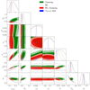 |
Fig. A.1. Marginalised posteriors distributions from the analysis of the WL and Clustering data sets. Each panel shows the posterior resulting from a separate analysis of clustering (green) and weak lensing (black) data sets as well as the combination of both data sets (red). Additionally, we show the Planck 2018 contours (Planck Collaboration VI 2020) for reference (blue). |
Our traditional constraints (i.e. with a single set of cosmological parameters governing geometry and growth) are in excellent agreement with the fiducial analyses of the band power spectra in Asgari et al. (2021), the BOSS DR12 consensus analysis in Alam et al. (2017) and the analysis of eBOSS DR14 data in Cuceu et al. (2019). Moreover, the Recomb data analysis recovers the Planck posterior for the parameters ns, As and θ*, as expected. The ns and As posteriors impose constraints along S8 or σ8, which are consistent with Planck constraints but significantly broader. Similarly, the θ* measurement imposes a degenerate constraint in the h − ωcdm plane, which contains the Planck 2018 contours (see Fig. A.3 for details). We observe that for the three combinations of KiDS data with external data sets, i.e ‘K1K+Clustering’, ‘K1K+Lyα’, and ‘K1K+CMB’, the posterior contours of the respective combined analysis fall at the intersection of the posteriors of the two individual data sets; see Figs. A.1, A.2, and A.3.
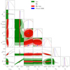 |
Fig. A.2. Marginalised posteriors distributions from the analysis of the WL and Ly-α data sets. Each panel shows the posterior resulting from a separate analysis of Lyman-α (green) and weak lensing (black) data sets as well as the combination of both data sets (red). Additionally, we show the Planck 2018 contours (Planck Collaboration VI 2020) for reference (blue). |
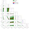 |
Fig. A.3. Marginalised posteriors distributions from the analysis of the WL and Recomb data sets. The Recomb data set is composed of data points for θ*, As, and ns which are inferred via marginalisation of the fiducial Planck posteriors (Planck Collaboration VI 2020) over the remaining cosmological parameters, as described in Section 3.4. Each panel shows the posterior resulting from a separate analysis of Recomb (green) and weak lensing (black) data sets as well as the combination of both data sets (red). Additionally, we show the Planck 2018 contours for reference (blue). |
Appendix B: Goodness of fit
In Table B.1 we provide the best-fit χ2-values, inferred from the maximum of the posterior, for each combination of data sets that we consider, and for both the split analysis of geometry and growth as well as the traditional analysis. Additionally, we show the number of free parameters employed in each of the analyses (nparams), as well as the associated number of data points (npoints). We note that in this work we adopted the fiducial KiDS-1000 cosmology covariance matrix. The fiducial results of Asgari et al. (2021), however, were obtained with an iterated covariance model which is based on the best-fit parameters of Heymans et al. (2021). While the covariance model has a negligible impact on the posteriors (see Asgari et al. 2021), it does impact the numerical χ2-value inferred from the maximum of the posterior at the few-percent level. Therefore, the best-fit χ2-values reported in Table B.1 are not directly comparable to the ones reported in Asgari et al. (2021).
Best-fit χ2 values for all different combinations of data sets considered.
It is common practice to assess the goodness of fit under the assumption that the χ2 statistic follows a χ2 distribution with the number of degrees of freedom DoF = npoints − nparams. The reduced χ2, that is defined by  , is then used as a measure of goodness of fit. However, this assumption requires that the data are normally distributed, that the model is linearly dependent on the sampling parameters, and that there is no informative prior on the parameter ranges (see for instance Joachimi et al. 2021). These conditions do not hold in general in cosmological analyses, which require a more sophisticated estimate of the effective number of degrees of freedom which can be inferred for example from mocks or posterior predictive data realisations (Andrae et al. 2010; Spiegelhalter et al. 2002; Handley & Lemos 2019b; Raveri & Hu 2019; Joachimi et al. 2021).
For the weak lensing data set used in this work, Joachimi et al. (2021) report an effective number of degrees of freedom of nparams, eff = 4.5. We cannot simply adopt this number since the split of cosmological parameters into two theory regimes and the addition of external data sets is expected to have an impact on the effective number of degrees of freedom. Therefore, we restrict the analysis to an interpretation of the commonly used approximation of the degrees of freedom as the difference between the number of data points and the number of parameters, that is conservative in identifying underfitting models. Nevertheless, we treat the five nuisance parameters that parameterise a shift in the mean of the five KiDS redshift bins as essentially fixed by their strongly informative Gaussian prior and thus we do not count them as free parameters.
The reduced χ2 for KiDS weak lensing is fairly high. As discussed in detail in Asgari et al. (2021), this result only occurs for the band power statistic and does not appear to point to a systematically underfitting model. We also applied our split analysis to an earlier KiDS data release (cf. Wright et al. 2019) and found consistent results with good χ2. The combination with any of the other data sets acts to reduce the reduced χ2 closer to unity, such that there is no sign of inconsistency between the probes we combine. We observe that the split analyses show a slightly better fit than their traditional counterparts represented by smaller values of χ2. However, comparing the reduced χ2, that takes the increased number of model parameters into account, we do not find a significant preference for the split model. Thus, we conclude that while the split model is better at fitting the data, such improvement is not decisive at justifying the extra added degrees of freedom with respect to the traditional analysis.
Moreover, we calculate the Bayes factor (Kass & Raftery 1995),
 (B.1)
(B.1)
where 𝒵 is the Bayesian evidence found for each model (see Eq. (14) for reference), as well as the difference between the Deviance Information Criterion (DIC; Gelman et al. 2004),
![Mathematical equation: $$ \begin{aligned} \mathrm{DIC} = \frac{1}{2} Var[\chi ^2]-\overline{\chi ^2}, \end{aligned} $$](/articles/aa/full_html/2021/11/aa41350-21/aa41350-21-eq75.gif) (B.2)
(B.2)
between the traditional and split model; ΔDIC = DICtrad − DICsplit, for each data set. The bar denotes the mean over the sampled χ2 values. Positive values of lnℬ correspond to more Bayesian evidence in support of the traditional model; negative values to preference for the split model. Models with a lower DIC are preferred by the data since they either possess a lower mean χ2 (i.e. a better fit of the data) or a lower variance in their χ2 (i.e. a lower effective number of parameters). Thus, the DIC acts as a combined measurement of goodness of fit and model complexity. Therefore, negative values of ΔDIC represent a preference for the traditional model while negative values support the split model.
The obtained values are shown in Table B.2. In order to asses the significance of the values reported by both metrics we follow the criteria laid out in Joudaki et al. (2017). We interpret −1 < lnℬ < 1 and DICtrad − DICsplit < 5 values as not to be significant enough to prefer either of the models. Therefore, we conclude that neither the Bayes factor nor the DIC show a preference for the split or the traditional model11.
Model comparison between the traditional and the split model, using the Bayes factor ℬ and the DIC.
Appendix C: Marginalised one-dimensional posterior distributions
In Fig. C.1 we provide the marginalised one-dimensional posteriors for h, Ωm, and σ8, corresponding to the posteriors shown in Fig. 2, for the combination of weak lensing, clustering, Lyman-α, and Recomb data sets. We note that due to how the constraining power is distributed in growth and geometry, growth h and geometry σ8 constraints are mostly prior-dominated.
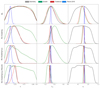 |
Fig. C.1. Marginalised one-dimensional posterior distributions of the cosmological parameters h (first column), Ωm (second column) and σ8 (third column) for different combinations of data sets (rows). The first row shows the constraints from the WL data set only, while the following rows show the constraints obtained when subsequently adding the Clustering, Ly-α, and Recomb data sets. In each panel we show a superposition of the constraints from our split analysis of growth and geometry theory regimes (green and grey contours respectively), a traditional analysis with one single set of cosmological parameters (red), and the Planck 2018 (Planck Collaboration VI 2020) constraints for reference (blue). |
Appendix D: Full cosmological posteriors
In this appendix we present the full set of posterior distributions for all cosmological parameters and for each of the studied combinations of data sets shown in Fig. 2. In Fig. D.1 we show the marginalised posterior in an analysis of weak lensing data, while Figs. D.2, D.3, and D.4 show the constraints in an analysis of weak lensing + clustering, weak lensing + clustering + Lyman-α, and weak lensing + clustering + Lyman-α + Recomb data, respectively. In each figure we provide the constraints on geometry and growth parameters from a split analysis of the two theory regimes (grey and green contours), as well the traditional analysis with one set of cosmological parameters (red). Additionally, we show the Planck 2018 contours (Planck Collaboration VI 2020) for reference (blue).
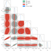 |
Fig. D.1. Marginalised posteriors from the analysis of the WL data set for all cosmological parameters. Each panel shows a superposition of the growth (green), geometry (grey), traditional analysis (red), and the Planck 2018 contours (Planck Collaboration VI 2020) for reference (blue). |
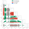 |
Fig. D.2. Marginalised posteriors from the analysis of the WL + Clustering data sets for all cosmological parameters. Each panel shows a superposition of the growth (green), geometry (grey), traditional analysis (red), and the Planck 2018 contours (Planck Collaboration VI 2020) for reference (blue). |
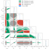 |
Fig. D.3. Marginalised posteriors from the analysis of the WL + Clustering + Ly-α data sets for all cosmological parameters. Each panel shows a superposition of the growth (green), geometry (grey), traditional analysis (red), and the Planck 2018 contours (Planck Collaboration VI 2020) for reference (blue). |
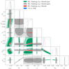 |
Fig. D.4. Marginalised posteriors from the analysis of the WL + Clustering + Recomb data sets for all cosmological parameters. Each panel shows a superposition of the growth (green), geometry (grey), traditional analysis (red), and the Planck 2018 contours for reference (blue). |
All Tables
Level of tension between traditional analysis and Planck for the parameters S8 and Ωm.
Model comparison between the traditional and the split model, using the Bayes factor ℬ and the DIC.
All Figures
|
Fig. 1. Schematic of the complete MONTEPYTHON 2COSMOS pipeline developed for the purposes of this work. Two instances of the cosmological code, cosmology 1 and cosmology 2, independently sample the cosmological parameters for the two theory regimes, geometry and growth, respectively. These parameters are then passed to the likelihood modules to calculate the theoretical prediction for each individual probe. Finally, the respective independent likelihood values for each probe are multiplied to obtain the likelihood value of the combined data set. |
| In the text | |
|
Fig. 2. Marginalised posterior distributions of σ8 and Ωm (top row), as well as h and Ωm (bottom row) for different combinations of data sets (columns). Each panel shows a superposition of four contours. Namely, the growth and geometry contours from the split analysis of the two theory regimes (green and grey contours respectively), the contour resulting from the traditional analysis with one set of cosmological parameters (red), and the reference contours from the Planck 2018 analysis (blue; Planck Collaboration VI 2020). |
| In the text | |
|
Fig. 3. Marginalised posterior for Ωm when comparing their geometry (horizontal axis) and growth (vertical axis) counterparts. We show the evolution of the contours as more data sources are added into the analysis. Namely, we display weak lensing (green), weak lensing combined with clustering data (grey), weak lensing combined with clustering and Lyman-α forest data (red) and finally weak lensing combined with clustering, Lyman-α forest and Recomb data (blue). |
| In the text | |
|
Fig. 4. Marginalised posterior distributions of the difference between geometry and growth parameter duplicates of S8, Ωm, and h. Each panel shows the contours for the combinations of data sets WL (green), WL + Clustering (black), WL + Clustering + Lyα (red) and WL + Clustering + Lyα + Recomb (blue). At the top-left corner of each panel we display the σ-level tension of each contour with respect to the null value pgrow = pgeom for all combination of data sets. |
| In the text | |
|
Fig. 5. S8 best-fit parameter values with their associated 1σ confidence regions obtained from the different combinations of data sets explored in this work. In top to bottom order we display the data sets WL, WL + Clustering, WL + Lyα, WL + Recomb, WL + Clustering + Lyα and finally WL + Clustering + Lyα + Recomb. The numerical value of the quantities displayed can be found in Table 5. |
| In the text | |
|
Fig. 6. Two-dimensional constraints for the combination of parameters Ωm − σ8 of the traditional analyses of Lyα+WL data (left) and of Recomb+WL (right). In both panels the empty black contours are the WL alone constraints while the filled blue ones are the Planck contours. Left panel: green contours show the Lyα constraints while the red contours show their combination with WL. Similarly, in the right panel: green contours show the Recomb constraints while the red contours show their combination with WL. The full posterior of these analyses can be seen in Figs. A.2 and A.3 respectively. |
| In the text | |
|
Fig. A.1. Marginalised posteriors distributions from the analysis of the WL and Clustering data sets. Each panel shows the posterior resulting from a separate analysis of clustering (green) and weak lensing (black) data sets as well as the combination of both data sets (red). Additionally, we show the Planck 2018 contours (Planck Collaboration VI 2020) for reference (blue). |
| In the text | |
|
Fig. A.2. Marginalised posteriors distributions from the analysis of the WL and Ly-α data sets. Each panel shows the posterior resulting from a separate analysis of Lyman-α (green) and weak lensing (black) data sets as well as the combination of both data sets (red). Additionally, we show the Planck 2018 contours (Planck Collaboration VI 2020) for reference (blue). |
| In the text | |
|
Fig. A.3. Marginalised posteriors distributions from the analysis of the WL and Recomb data sets. The Recomb data set is composed of data points for θ*, As, and ns which are inferred via marginalisation of the fiducial Planck posteriors (Planck Collaboration VI 2020) over the remaining cosmological parameters, as described in Section 3.4. Each panel shows the posterior resulting from a separate analysis of Recomb (green) and weak lensing (black) data sets as well as the combination of both data sets (red). Additionally, we show the Planck 2018 contours for reference (blue). |
| In the text | |
|
Fig. C.1. Marginalised one-dimensional posterior distributions of the cosmological parameters h (first column), Ωm (second column) and σ8 (third column) for different combinations of data sets (rows). The first row shows the constraints from the WL data set only, while the following rows show the constraints obtained when subsequently adding the Clustering, Ly-α, and Recomb data sets. In each panel we show a superposition of the constraints from our split analysis of growth and geometry theory regimes (green and grey contours respectively), a traditional analysis with one single set of cosmological parameters (red), and the Planck 2018 (Planck Collaboration VI 2020) constraints for reference (blue). |
| In the text | |
|
Fig. D.1. Marginalised posteriors from the analysis of the WL data set for all cosmological parameters. Each panel shows a superposition of the growth (green), geometry (grey), traditional analysis (red), and the Planck 2018 contours (Planck Collaboration VI 2020) for reference (blue). |
| In the text | |
|
Fig. D.2. Marginalised posteriors from the analysis of the WL + Clustering data sets for all cosmological parameters. Each panel shows a superposition of the growth (green), geometry (grey), traditional analysis (red), and the Planck 2018 contours (Planck Collaboration VI 2020) for reference (blue). |
| In the text | |
|
Fig. D.3. Marginalised posteriors from the analysis of the WL + Clustering + Ly-α data sets for all cosmological parameters. Each panel shows a superposition of the growth (green), geometry (grey), traditional analysis (red), and the Planck 2018 contours (Planck Collaboration VI 2020) for reference (blue). |
| In the text | |
|
Fig. D.4. Marginalised posteriors from the analysis of the WL + Clustering + Recomb data sets for all cosmological parameters. Each panel shows a superposition of the growth (green), geometry (grey), traditional analysis (red), and the Planck 2018 contours for reference (blue). |
| In the text | |
Current usage metrics show cumulative count of Article Views (full-text article views including HTML views, PDF and ePub downloads, according to the available data) and Abstracts Views on Vision4Press platform.
Data correspond to usage on the plateform after 2015. The current usage metrics is available 48-96 hours after online publication and is updated daily on week days.
Initial download of the metrics may take a while.