| Issue |
A&A
Volume 653, September 2021
|
|
|---|---|---|
| Article Number | A36 | |
| Number of page(s) | 28 | |
| Section | Extragalactic astronomy | |
| DOI | https://doi.org/10.1051/0004-6361/202140696 | |
| Published online | 07 September 2021 | |
Calibration of mid- to far-infrared spectral lines in galaxies
1
Dipartimento di Fisica, Università di Roma La Sapienza, P.le A. Moro 2, 00185 Roma, Italy
e-mail: This email address is being protected from spambots. You need JavaScript enabled to view it.
2
Istituto di Astrofisica e Planetologia Spaziali (INAF–IAPS), Via Fosso del Cavaliere 100, 00133 Roma, Italy
e-mail: This email address is being protected from spambots. You need JavaScript enabled to view it.
, This email address is being protected from spambots. You need JavaScript enabled to view it.
Received:
1
March
2021
Accepted:
6
May
2021
Abstract
Context. Mid- to far-infrared (IR) lines are suitable in the study of dust-obscured regions in galaxies because dust extinction strongly decreases with wavelength, and therefore IR spectroscopy allows us to explore the most hidden regions of galaxies, where heavily obscured star formation as well as accretion onto supermassive black holes at the nuclei of galaxies occur. This is mostly important for the so-called cosmic noon (i.e. at redshifts of 1 < z < 3), at which point most of the baryonic mass in galaxies has been assembled.
Aims. Our goal is to provide reliable calibrations of the mid- to far-IR ionic fine-structure lines, the brightest H2 pure rotational lines, and the polycyclic aromatic hydrocarbon (PAH) features, which we used to analyse current and future observations in the mm-submm range from the ground, as well as mid-IR spectroscopy from the upcoming James Webb Space Telescope.
Methods. We used three samples of galaxies observed in the local Universe: star-forming galaxies (SFGs, 196), active galactic nuclei (AGN; 90−150 for various observables), and low-metallicity dwarf galaxies (40). For each population, we derive different calibrations of the observed line luminosities versus the total IR luminosities.
Results. Through the resulting calibrations, we derive spectroscopic measurements of the star formation rate (SFR) and of the black hole accretion rate (BHAR) in galaxies using mid- and far-IR fine-structure lines, H2 pure rotational lines and PAH features. In particular, we derive robust star formation tracers based on the following: the [CII]158 μm line; the sum of the two far-IR oxygen lines, the [OI]63 μm line, and the [OIII]88 μm line; a combination of the neon and sulfur mid-IR lines; the bright PAH features at 6.2 and 11.3 μm; as well as – for the first time – the H2 rotational lines at 9.7, 12.3, and 17 μm. We propose the [CII]158 μm line, the combination of the two neon lines ([NeII]12.8 μm and [NeIII]15.5 μm), and, for solar-like metallicity galaxies that may harbour an AGN, the PAH 11.3 μm feature as the best SFR tracers. On the other hand, a reliable measure of the BHAR can be obtained using the [OIV]25.9 μm and the [NeV]14.3 and 24.3 μm lines. For the most commonly observed fine-structure lines in the far-IR, we compare our calibration with the existing ALMA observations of high-redshift galaxies. We find an overall good agreement for the [CII]158 μm line for both AGN and SFGs, while the [OIII]88 μm line in high-z galaxies is in better agreement with the low-metallicity local galaxies (dwarf galaxy sample) than with the SFGs, suggesting that high-z galaxies might have strong radiation fields due to low metal abundances, as expected.
Key words: galaxies: active / galaxies: evolution / galaxies: star formation / infrared: galaxies / techniques: spectroscopic
© ESO 2021
1. Introduction
One of the major and still unsolved problems in astrophysics is the lack of a clear understanding of how galaxies evolve, from the time of structure formation to the present day, and the dominant processes that influence their evolution (Somerville & Davé 2015; Naab & Ostriker 2017; Bullock & Boylan-Kolchin 2017; Wechsler & Tinker 2018; Förster Schreiber & Wuyts 2020). From the observational scenario that has been consolidated in the last several tens of years, we know that the two main energy production mechanisms in galaxy evolution are, on one side, star formation and subsequent stellar evolution, and, on the other side, accretion onto the supermassive black holes (SMBHs) that form at the centre of a galaxy.
The bulk of star formation and black hole (BH) accretion took place at the so-called cosmic noon (1 < z < 3) with a steep decline towards the present epoch. This occurred in heavily obscured environments, embedded in large amounts of gas and dust where optical and UV detected radiation corresponds to only ∼10% of the total emitted light (Madau & Dickinson 2014) and with most of the radiated energy being absorbed by dust and re-emitted at longer wavelengths. Both star formation and black hole accretion contribute to the dust re-emission. Therefore, measuring the integrated IR continuum through photometric observations does not allow us to easily differentiate between the two components. The spatial resolution required to isolate the bulk of the nuclear IR emission from the host galaxy (≲100 pc) cannot be attained in high-z galaxies, while spectral decomposition techniques (e.g., Berta et al. 2013) are ultimately dependent on templates of local active galactic nuclei (AGN), whose inner workings and dust distribution are still far from being understood (e.g. Lyu & Rieke 2021). Thus measuring star formation rate (SFR) and black hole accretion rate (BHAR) in galaxies across cosmic time, which is one of the major observational goals in galaxy evolution studies, has to be done through spectroscopic observations at wavelengths long enough to overcome dust absorption.
The mid- to far-IR range is populated by a large number of atomic and molecular lines and features. In particular, the atomic and ionic fine-structure lines cover a wide range of physical parameters in terms of excitation, density, and ionisation, as can be seen in Fig. 4 of Spinoglio et al. (2012), which shows the critical density for collisional de-excitation versus the ionisation potential of the IR fine-structure lines. These lines can easily discriminate among the different gas excitation conditions, from the narrow line regions (NLR) excited by the active nucleus, to the H II and photo-dissociation regions (PDRs), whose origin is due to stellar excitation (see e.g. Spinoglio & Malkan 1992; Tommasin et al. 2010; Spinoglio et al. 2015; Fernández-Ontiveros et al. 2016), offering an ideal tool to probe the highly opaque and dust-obscured regions. Most of these lines can be assessed only from space IR telescopes, while only a few transitions happen to lie in the atmospheric windows; for example, in the spectral region of 8 − 13 μm.
The intermediate ionisation fine-structure lines are good tracers of the star formation, and the sum of the fluxes of [NeII] and [NeIII] has in particular been shown to give a measure of the star formation rate (Ho & Keto 2007; Zhuang et al. 2019) in galaxies. The low-ionisation [CII] line at 158 μm is one of the brightest emission lines in star-forming galaxies (SFGs), and it can thus trace star formation activity both in the local (De Looze et al. 2014; Herrera-Camus et al. 2015) and high-redshift (Leung et al. 2020) Universe.
The mid-IR spectra of SFGs between 3 and 19 μm are often dominated by emission features attributed to polycyclic aromatic hydrocarbons (PAHs), due to infrared (IR) fluorescence by these large molecules containing 50−100 C-atoms, pumped by single FUV photons (Allamandola et al. 1989; Smith et al. 2007; Tielens 2008). Because they trace the FUV stellar flux, they can be used to measure star formation. These features are strong when compared to fine-structure lines in SFGs, and are detected not only in local galaxies, but also at redshifts up to z ∼ 4 (Kirkpatrick et al. 2015; Riechers et al. 2014; Sajina et al. 2012). Their emission accounts for ∼10 − 20% of the total IR radiation by dust, and originate from PDRs near star forming regions. PAHs can be used to trace SFRs not only in SFGs (Shipley et al. 2016; Xie & Ho 2019), but also in sources where an AGN contribution is present but not the dominant source of integrated light (Shipley et al. 2013). In these AGN, the equivalent width of the PAH features can be used to estimate the star formation contribution to the total IR luminosity (Armus et al. 2007; Tommasin et al. 2010). However, in more extreme AGN, strong UV and X-ray radiation fields can also suppress the PAH emission in the vicinity of the AGN by photo-dissociation, while increasing the mid-IR continuum emission (Lacy et al. 2013). Analogously, in low metallicity galaxies (LMGs; i.e. below 12 + log(O/H) ∼ 8.2), because of the reduced formation efficiency and the increased stellar radiation hardness, the strength of the PAH features is reduced and only detected at metallicities above 1/8−1/10 Z⊙ (Engelbracht et al. 2008; Cormier et al. 2015; Galliano et al. 2021).
Among the molecular lines in the mid-IR, the pure rotational transitions of H2 are particularly important as the typical physical conditions of the gas associated with these lines can be found both in AGN and SFGs. Rigopoulou et al. (2002) found that while in star forming environments the H2 emission can originate from PDRs (with a small contribution from shocks), in AGN-dominated galaxies the X-ray emission from the central AGN plays an important role in heating large amounts of gas boosting the H2 emission.
High ionisation lines trace AGN activity: all lines whose ionisation potential is higher than the one necessary to doubly ionise helium (> 54.4 eV) cannot be efficiently produced by stellar radiation in significant amounts. Therefore, the detection of the [NeV]14.3 μm, [NeV]24.3 μm or [NeVI]7.65 μm lines probes the presence of an AGN, while the [OIV]25.9 μm line, which can also be found in energetic starbursts and LMGs, is however much stronger in AGN, having an equivalent width one order of magnitude larger compared to SFGs (Tommasin et al. 2010). Typical IR line ratios used to measure the strength of the active nucleus with respect to the star formation component in a galaxy are the [NeV]14.3 μm or 24.3 μm to [NeII]12.8 μm ratio, the [OIV]25.9 μm/[NeII]12.8 μm line ratio, and the [OIV]25.9 μm/[OIII]52 μm or 88.35 μm ratio (Sturm et al. 2002; Armus et al. 2007; Tommasin et al. 2010; Spinoglio et al. 2015; Fernández-Ontiveros et al. 2016).
The main goals of this work are (i) to revise the calibration of the mid- to far-IR lines including ionic fine-structure lines, the brightest H2 pure rotational lines and the PAH features; and (ii) to provide a local calibration of spectroscopic SFRs and BHAR tracers, which can also be applied to measurements at high-z. We follow the study presented in Spinoglio et al. (2012), update the IR spectroscopic observations presented there, and include a sample of LMGs to extend the calibration to these objects. The latter two are included to characterise the response of the lines to the conditions of low metallicity (average 1/5 Z⊙) (Madden et al. 2013). Low-metallicity AGN are not included because they are rare in the local Universe and only a few examples are found (e.g. Circinus, Oliva et al. 1999), but the broad- and narrow-line regions in AGN essentially show little or no chemical evolution up to z ∼ 7 (Nagao et al. 2006; Juarez et al. 2009; Onoue et al. 2020), suggesting that the quasar phase appears mostly when galaxies are already chemically mature objects. Therefore, including the metallicity dependence in the calibrations for AGN is not as relevant as it is in the case of SFGs, where the chemical evolution with redshift is well known (Sanders et al. 2021). This work extends and updates a previous study (Spinoglio et al. 2021) aimed to prepare for the SPICA mission (Roelfsema et al. 2018) where the authors give a calibration of the most important features that were used to plan spectroscopic observations with that mission.
A further motivation for this study is the need to exploit the great potential of extragalactic IR spectroscopy for high-redshift galaxies, which is already being explored by the Atacama Large Millimetre sub-millimetre Array (ALMA, Wootten & Thompson 2009; Carpenter et al. 2020) and will benefit from a dramatic boost with the next space IR telescopes, such as the James Webb Space Telescope (JWST, Gardner et al. 2006), and in the more distant future, possibly by the Origins Space Telescope1.
The paper is organised as follows: Sect. 2 describes the samples of galaxies, observed in the local Universe, that we have used to derive the correlations; Sect. 3 reports our results, and in particular Sect. 3.1 presents the new correlations between the line luminosities and the total IR luminosities, while Sects. 3.2 and 3.3 give simple methods to measure the two main parameters of the SFR and BHAR. In Sect. 4, we discuss our results, and Sect. 4.3 compares our study to previous ones. In Sect. 4.4, we discuss the metallicity effect on the SFR tracers, while Sect. 4.5 presents how the observations at high redshift compare with the correlations we derive. Section 4.6 shows how our results can be used to interpret present and future IR and (sub)-mm observations. Our conclusions are presented in Sect. 5.
2. Selected lines and features and samples of galaxies
We used the most representative samples of SFGs, AGN, and LMGs in the local Universe for which IR spectroscopy is available, mainly from Spitzer-IRS (Houck et al. 2004) and Herschel-PACS (Poglitsch et al. 2010), but also from the Infrared Space Observatory’s (ISO) SWS and LWS spectrometers (de Graauw et al. 1996; Clegg et al. 1996). For each of the three galaxy populations, we derived linear relations in logarithmic space between the line luminosity and the total IR luminosity. Then we derived the best tracers of the SFR and the BHAR, using the discussed IR lines and features, and compared them with what has been reported in the literature.
In this analysis, we considered the following, in order of decreasing ionisation or excitation:
-
Four high-ionisation fine-structure lines, typical of AGN: [NeVI]7.65 μm, [NeV]14.32 μm, [NeV]24.32 μm and [OIV]25.89 μm;
-
Ten intermediate ionisation fine-structure lines, typical of stellar or H II regions: [SIV]10.51 μm, [NeII]12.81 μm, [NeIII]15.55 μm, [SIII]18.71 μm, [SIII]33.48 μm, [OIII]51.81 μm, [NIII]57.32 μm, [OIII]88.36 μm, [NII]121.9 μm, and [NII]205 μm;
-
Five low-ionisation and neutral fine-structure lines, typical of PDR: [FeII]25.99 μm, [SiII]34.81 μm, [OI]63.18 μm, [OI]145.5 μm, and [CII]157.7 μm;
-
Four H2 pure rotational lines at 9.67, 12.28, 17.03, and 28.22 μm;
-
Five PAH features at 6.2, 7.7, 8.6, 11.3, and 17 μm.
The fundamental parameters for the fine-structure lines considered in this analysis are reported in Table A.1.
In this analysis, we included those lines observed with the Spitzer-IRS high-resolution (HR) channel in the 10−35 μm range, for which good spectra are available in the literature. The only exception is the line of [NeVI]7.65 μm, an exclusive AGN line, for which we included ISO-SWS observations. Other well-known fine-structure lines, such as [ArII]6.98 μm, [ArIII]8.99 μm, and [NeIII]36.0 μm, which could indeed play a relevant role in future observations, especially in view of the JWST launch, do not have enough high-quality spectra in the literature to be included in the analysis at the present time. We did not consider upper limits to derive our correlations. This is because, in general, our statistics are quantitatively appropriate, thus making the inclusion of upper limits not necessary. Moreover, where the statistics are less precise, upper limits are usually not available for the considered lines. The definition of the various samples of galaxies chosen to compute the correlations are described in the following sections and summarised in Table 1, with the instruments used to observe the spectral lines and features, the total number of objects selected and the references for each sample.
Characteristics of the samples associated with the different spectral classes used in this analysis.
2.1. The AGN sample
The AGN sample has been drawn from the 12 μm selected active galaxies sample (12MGS, Rush et al. 1993), which is the brightest complete and unbissed sample of Seyfert galaxies in the local Universe. For the mid-IR fine-structure lines and the H2 rotational lines, we have used the sub-sample of the 12MGS observed by Spitzer-IRS at high spectral resolution (R = 600) which contains 88 AGN (Tommasin et al. 2008, 2010). For the PAH features at 6.2 μm and 11.2 μm we have used the Spitzer-IRS data at low spectral resolution (R ∼ 60 − 120; Buchanan et al. 2006; Wu et al. 2009) of the 12MGS (103 objects), because this setting matches better the intrinsic width of these features. We note here that Wu et al. (2009) measure the PAH features using a spline function to determine the continuum level. In order to make these measurements comparable to those obtained using automated fitting procedures (e.g. PAHFIT, Smith et al. 2007), we applied a correction factor of 1.7 and 1.9 to increase the fluxes of the 6.2 μm and 11.3 μm PAH in Wu et al. (2009), respectively, following the differences found by Smith et al. (2007). The adoption of the complete 12MGS as the main catalog, from which we covered about 75% of the total sample, allowed us to derive statistically robust calibrations.
For the [NeVI]7.65 μm line, we could not use the 12MGS, because this line was not detected by Spitzer at low resolution and was outside its spectral range at high-resolution. Therefore we had to use the data from Sturm et al. (2002), which contain 8 detections of the [NeVI]7.65 μm line with ISO-SWS at medium resolution (R ∼ 1500), and thus not contaminated by the PAH emission at 7.7 μm.
For the far-IR spectral range, namely the 50 − 205 μm, we used the catalogue of AGN assembled by Fernández-Ontiveros et al. (2016), which includes all the Seyfert galaxies and the quasars of the Véron-Cetty & Véron (2010) catalogue, which have far-IR spectra observed by Herschel-PACS. The sample of the AGN observed in the far-IR lines counts 170 galaxies and contains about 50% of objects from the 12MGS, while the others do not come from a complete sample.
2.2. The SFG sample
The SFG sample was constructed using the Great Observatories All-Sky LIRG Survey (GOALS sample, Armus et al. 2009), from which we extracted 158 galaxies, with data from Inami et al. (2013), who report the fine-structure lines at high resolution in the 10 − 36 μm interval, and Stierwalt et al. (2014), who include the detections of the H2 molecular lines and the PAH features at low spectral resolution. For those galaxies in the GOALS sample that have a single IRAS counterpart, but more than one source detected in the emission lines, we have added together the line or feature fluxes of all components, to consistently associate the correct line or feature emission to the total IR luminosity computed from the IRAS fluxes. To also cover lower luminosity galaxies, as the GOALS sample only includes luminous IR galaxies (LIRGs) and ultra-luminous IR galaxies (ULIRGs), we included 38 galaxies from Bernard-Salas et al. (2009) and Goulding & Alexander (2009), to reach the total sample of 196 galaxies with IR line fluxes in the 5.5 − 35 μm interval in which an AGN component is not detected. For the Bernard-Salas et al. (2009), Goulding & Alexander (2009), and the GOALS samples, we excluded all the composite starburst-AGN objects identified as those with a detection of [NeV] either at 14.3 or 24.3 μm. It is worth noting that the original samples from Goulding & Alexander (2009) and Bernard-Salas et al. (2009) have spectra solely covering the central region of the galaxies. To estimate the global SFR, we corrected the published line fluxes of the Spitzer spectra by multiplying them by the ratio of the continuum reported in the IRAS point source catalogue to the continuum measured on the Spitzer spectra extracted from the CASSIS database (Lebouteiller et al. 2015). We assumed here that the line emission scales (at first order) with the IR brightness distribution. In particular, we considered the continuum at 12 μm for the [NeII]12.8 μm and [NeIII]15.6 μm lines, and the continuum at 25 μm for the [OIV]25.9 μm, [FeII]26 μm, [SIII]33.5 μm, and [SiII]34.8 μm lines. This correction was not needed for the AGN sample and the GOALS sample because of the greater average redshift of the galaxies in the 12MGS and GOALS samples. In particular, the 12MGS active galaxy sample has a mean redshift of 0.028 (Rush et al. 1993), while the GOALS sample has a mean redshift of 0.026. The galaxies presented by Bernard-Salas et al. (2009) have instead an average redshift of 0.0074, while the sample by Goulding & Alexander (2009) has an average redshift of 0.0044. For the other lines in the 10 − 36 μm interval, Goulding & Alexander (2009) did not report a detection, and we used the data presented in Bernard-Salas et al. (2009) for a total of 15 objects. Both Bernard-Salas et al. (2009) and Goulding & Alexander (2009) reported data from the high-resolution Spitzer-IRS spectra. Data in the 50 − 205 μm interval were taken from Díaz-Santos et al. (2017). For the GOALS sample, 20 starburst galaxies were taken from Fernández-Ontiveros et al. (2016), and 23 objects were taken from the ISO-LWS observations of Negishi et al. (2001). As a result, we obtained a total sample of 193 objects. Lastly, the PAH features’ fluxes were measured from the low-resolution Spitzer-IRS spectra by Brandl et al. (2006), including 12 objects from the sample of Bernard-Salas et al. (2009) and 179 objects from Stierwalt et al. (2014).
2.3. The LMG sample
The LMG sample was selected from Cormier et al. (2015), where the 10 − 36 μm interval was observed by Spitzer-IRS in both high and low resolutions, and the 50 − 158 μm interval was observed by Herschel-PACS. For the Spitzer-IRS data, we only considered the high-resolution results, for a total sample of 40 objects.
3. Results
We derived, for each line or feature in each galaxy sample, the correlation between the logarithms of the total IR luminosity in the 8 − 1000 μm range – computed from the IRAS fluxes following Sanders & Mirabel (1996) – and the line luminosity, according to the following equation:
 (1)
(1)
with all luminosities expressed in units of 1041 erg s−1. We report in Table D.1 the best-fit parameters obtained for each line or feature using the orthogonal distance regression fit (Boggs & Rogers 1990), the number of objects N, and the Pearson correlation coefficient r. We used the orthogonal distance regression because the two variables are independent of each other, instead of the ordinary least-squares minimisation, where one variable is dependent on the other one. This is also particularly useful to derive the inverse relation between the two variables from the best-fit coefficients.
Using these correlations, we derived the tracers for the SFR (Sect. 3.2) and the BHAR (Sect. 3.3). For the SFR, we used the [CII]158 μm luminosity, various combinations of the luminosities of the [NeII]12.8 μm, [NeIII]15.6 μm, [SIII]18.7 μm and [SIV]10.5 μm lines, the luminosity of the PAH features at 6.2 μm, and 11.3 μm and the luminosity of the H2 rotational lines at 9.7 μm, 12.3 μm, and 17.3 μm. For the BHAR, we used the luminosities of the [OIV]25.9 μm, [NeV]14.3 μm and 24.3 μm lines.
3.1. Spectral lines and features versus total IR luminosity
Among the different correlations derived in this work and presented in Table D.1, in this section we highlight the main results, while we refer the reader to Appendix B for the whole set of figures illustrating the correlations with the total IR luminosity. In Fig. 1a, we present the correlation between the [CII]158 μm line luminosity and the total IR luminosity for the three galaxy populations considered. We find that the SFG and the LMG samples follow a tight relation over six orders of magnitude in LIR with a consistent regression slope and offset values within the uncertainties, from low-luminosity dwarf galaxies to LIRGs and ULIRGs, confirming the results of De Looze et al. (2014). This is further discussed in Sect. 3.2.2. On the other hand, AGN have higher IR luminosities for a given [CII]158 μm line luminosity with respect to the SFG and LMG samples, likely due to the contribution of the AGN continuum emission to the total IR luminosity. This effect is also seen in low-ionisation transitions where the AGN contribution to the line emission is expected to be small, such as the [NII]122 μm line (see Fig. 1c). However, the same effect is not observed for [OI]63 μm (see Fig. B.7b). This might be related to the higher critical density of the [OI]63 μm line, which becomes an efficient coolant in X-ray dissociation regions in the presence of an AGN (Maloney et al. 1996; Dale et al. 2004). High-excitation lines where the AGN completely dominates the line emission show the opposite behaviour, that is, the sources are shifted towards higher line intensities at a given IR luminosity (e.g. [OIV]25.9 μm in Fig. 2b). This suggests that the lack of a noticeable shift between AGN and SFGs in intermediate excitation lines such as [NeII]12.8 μm or [SIII]18.7,33.5 μm (Figs. 1b, B.4b and B.6a) might be caused by a comparable AGN contribution to both the IR luminosity and the line intensity.
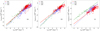 |
Fig. 1. a: [CII]158 μm line luminosity as a function of the total IR luminosity. Blue squares represent detections in AGN, red stars indicate SFGs, and green triangles LMGs. The solid red line represents the linear relation calculated for SFGs, the blue dotted line shows the relation for AGN, and the green dashed line the one for LMGs. b: [NeII]12.8 μm line luminosity as a function of the total IR luminosity. c: [NeIII]15.6 μm line luminosity as a function of the total IR luminosity. In b and c, we use the same notations as in a. |
We note that various authors (e.g. Herrera-Camus et al. 2015; Croxall et al. 2017) have reported an observed deficit in [CII] luminosity with the increase of total LIR, in particular in ULIRGs. Different mechanisms have been proposed to explain the lower [CII] emission (Sutter et al. 2019, 2021, and references therein). In particular, Sutter et al. (2019) found that the [CII] deficit is particularly evident when the emission arises from ionised gas, while the effect is negligible when the emission comes predominantly from PDR regions.
For the [NeII]12.8 μm line (Fig. 1b) there is a slight difference between SFGs and the other samples, but the differences are consistent within 3σ of each other and thus not statistically relevant.
In Fig. 1c, we report the correlation obtained for the [NeIII]15.6 μm line with the total IR luminosity, showing that the AGN and the SFGs have a comparable correlation, while LMGs have the [NeIII]15.6 μm line more than one order of magnitude brighter, at a given IR luminosity (see also Cormier et al. 2012).
In Figs. 2a–c, we report the correlations obtained for the [OIII]88 μm, the [OIV]25.9 μm line luminosities and the luminosity of the PAH feature at 11.3 μm with the total IR luminosity, respectively. For the [OIII]88 μm line, LMGs are on average two orders of magnitude brighter, at a given IR luminosity (see also Cormier et al. 2012), compared to the other two classes of galaxies, which are almost overlapping. This could be due to the differences in the ionising spectra and conditions in the ISM of LMGs with respect to the SFGs and the AGN. In LMG, an increased number of photons can ionise gas at greater distances from the star forming regions, thus facilitating cooling through ionised gas emission. Additionally, the lower dust-to-gas ratios in LMGs are also expected to cause a decrease of the IR luminosities, at a fixed stellar mass, in these galaxies.
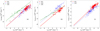 |
Fig. 2. a: [OIII]88 μm line luminosity as a function of the total IR luminosity. b: [OIV]25.9 μm line luminosity as a function of the total IR luminosity. c: luminosity of the PAH feature at 11.3 μm as a function of the total IR luminosity. The same legend as in Fig. 1 was used. |
AGN have about one order of magnitude brighter [OIV]25.9 μm emission compared to SFGs (see also Tommasin et al. 2010), and LMGs have a shallower relation with IR luminosity, with a decreasing slope at higher luminosities (Fig. 2b). The flatter slope could be related to the high-ionisation potential of the [OIV]25.9 μm line, that is, the few ionising photons beyond 54.4 eV produced by LMGs might not scale linearly with the overall luminosity. However, no firm conclusion can be drawn because of the relatively poor LMG statistics, for which only 16 detections of the [OIV] line are available. We note here that in order to obtain a reliable correlation for the AGN sample, we only considered objects with an AGN component at the 19 μm continuum greater than 85%, as defined in Tommasin et al. (2010). We only applied this limit in this case, to minimise a possible contamination in this line from emission due to strong starburst activity (see e.g. Lutz et al. 1998). This approach is motivated by the use of the [OIV]25.9 μm line as a BHAR tracer in Sect. 3.3, where the same reduced sample is adopted.
Figure 2c shows that the 11.3 μm PAH feature is present both in AGN and SFG and correlates well with the total IR luminosity, while in this analysis we do not consider the PAH detections in LMG, because detections are only available in a few cases, and thus are not enough to obtain a statistically significant result. As shown by different authors (Madden 2000; Engelbracht et al. 2005; Wu et al. 2006; Smith et al. 2007; Calzetti et al. 2007), in LMGs there is evidence of a PAH emission deficit, and the available measurements present significantly weaker features than SFGs. Moreover, the higher ionising continuum present in LMGs contribute to the destruction of these features (Engelbracht et al. 2008; Cormier et al. 2015). As we show in Sect. 3.2.5, while there is a difference of ∼0.3 dex between the emission of SFG and AGN, the slopes of the two correlations are comparable within the errors, with the difference linked to a higher LIR for equal PAH emission in AGN.
We note that while in Table D.1 we report the correlation derived for the [NeVI]7.6 μm line, this correlation was obtained for a sample of only eight AGN, while for the majority of AGN this line is not detected. We therefore conclude that this calibration has to be taken with caution, because it may be biassed in favour of AGN with a high-ionisation parameter (U ∼ −1), while for a lower ionisation we expect the [NeVI] line to be considerably less prominent, as discussed in Satyapal et al. (2021, in particular in their Fig. 5).
3.2. Star formation rate tracers
3.2.1. Determination of SFR
In this section, we propose different SFR tracers. In order to calibrate the proposed SFR tracers, we use two different methods. For SFGs, we measure the SFR directly from the total IR luminosity LIR, following Kennicutt (1998):
 (2)
(2)
where kIR = 4.5 × 10−44 M⊙ yr−1 erg−1 s. We apply the same conversion to AGN sources (see Sect. 3.2.5), but we limit our sample to the sources with LIR ≤ 1045 erg s−1. We apply this limit to minimise the AGN effect on the LIR and to avoid overestimating the SFR because of AGN activity.
For the LMGs, we adopted the SFR derived from Hα and corrected by the total IR luminosity, as reported in Rémy-Ruyer et al. (2015). The total IR luminosity alone does not accurately represent the total SFR in LMG due to the lower dust-to-gas ratio in their ISM. The inclusion of the optical component for computing the SFR is necessary to properly account for the emission not reprocessed by dust.
3.2.2. L[CII]158 μ[sans]m–SFR relation
The [CII]158 μm line can be used as a tracer of the SFR, as proposed by different authors (see e.g. De Looze et al. 2014). We compare the line intensity of SFGs and LMGs to the SFR. Applying the orthogonal distance regression fit, we find a strong correlation between the following two quantities:
![Mathematical equation: $$ \begin{aligned} \log \left(\frac{\mathrm{SFR}}{{M}_{\odot }\,\mathrm{yr}^{-1}}\right)=&(0.62 \pm 0.02)\nonumber \\&+(0.89 \pm 0.02) \left(\log \frac{L_{\rm [CII]}}{10^{41}\,\mathrm{erg\,s}^{-1}}\right)\cdot \end{aligned} $$](/articles/aa/full_html/2021/09/aa40696-21/aa40696-21-eq3.gif) (3)
(3)
In Fig. 3a, we show the correlation obtained for 227 galaxies, 37 of which are LMGs and 190 are SFGs. The relation is nearly linear, with a Pearson r value of r = 0.92, and it covers six orders of magnitude in SFR, indicating that the [CII] line emission is an overall good tracer of SFR for local SFGs independently of their metallicity. We excluded the AGN from this correlation, since we derived the SFR from the LIR and AGN have an excess IR continuum emission not due to star formation.
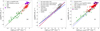 |
Fig. 3. a: correlation between the [CII]158 μm line luminosity and the SFR derived from the total LIR. Red stars represent SFG, and green triangles represent the LMG. Purple squares show the ULIRG population of SFG, and the shaded green area indicates the 95% confidence interval. b: comparison of the log L[CII]–log(SFR) relation obtained in this work (black solid line) with the results obtained by De Looze et al. (2014); the green dashed line represents a sample of HII or SFGs, the blue diamond line shows the results for the low-metallicity dwarf sample, and the pink dash-dotted line considers the whole sample. The red dotted line shows the results obtained by Sargsyan et al. (2012). c: correlation between the [NeII]12.8 μm and [NeIII]15.6 μm summed emission lines’ luminosity, in units of 1041 erg s−1, and the SFR derived from the total IR luminosity (black dashed line) for SFGs (red star) and from the Hα luminosity (corrected for the IR luminosity) for LMGs (green triangles). The shaded green area indicates the 95% confidence interval. The purple squares highlight the ULIRG population in the SFG sample. The blue dashed line shows the results obtained by Zhuang et al. (2019) for the same relation. |
In Fig. 3b, we compare our results with those obtained in De Looze et al. (2014) and Sargsyan et al. (2012). We note that, while in this work and in the work by Sargsyan et al. (2012) the SFR was determined following Kennicutt (1998), De Looze et al. (2014) traced the SFR using the GALEX FUV emission (Cortese et al. 2012) and the Spitzer–MIPS 24 μm emission (Rieke et al. 2004). When compared to the results obtained by De Looze et al. (2014) for their total sample, we find good agreement at luminosities of L[CII] > 1041 erg s−1, while there is a difference of ∼0.3 dex for lower luminosities. In De Looze et al. (2014), the dwarf sample, when considered alone, shows a flatter slope than the total sample, equal to 0.80 ± 0.5 (see Fig. 3b, blue diamond line). The authors link the flatter slope to an underestimation of the SFR based on the far-UV emission. We observe a similar flattening of the slope when considering the LMG sample alone, equal to 0.69 ± 0.05, consistent with the result by De Looze et al. (2014) within 3σ of each other.
De Looze et al. (2014) found that the ULIRG population presents a scatter of almost one order of magnitude in the [CII]–SFR relation, when compared to the total sample. We find the same result in our correlation, with the ULIRG population (composed of 16 objects) lying between 0.2 and 1.0 dex above the correlation derived for the total sample. Given the small number of sources, we do not derive a specific [CII]–SFR correlation for the ULIRG sample.
3.2.3. Oxygen-based SFR tracer
Besides C+, O and O2+ are two important coolants of the ISM. The [OI]63 μm line traces the warm and/or dense PDRs, while the [OIII]88 μm emission line originates from diffuse, highly ionised regions near young, hot stars.
The [OIII] line can be an important SFR tracer in an LMG (De Looze et al. 2014), where PDRs are weak or absent in the ISM and the ionisation field is stronger. In order to trace the SFR in an SFG, however, a tracer that can account for PDRs needs to be included. For this reason, combining these two lines can provide an accurate estimate of the SFR, both in SFGs and LMGs, probing both neutral and ionised media.
Figure 4 shows the correlation obtained for a sample of 151 objects, 24 LMGs, and 124 SFGs, 22 of which are ULIRGs. The correlation, with a Pearson correlation coefficient of r = 0.94, can be expressed by
![Mathematical equation: $$ \begin{aligned} \log \left(\frac{\mathrm{SFR}}{{M}_{\odot }\,\mathrm{yr}^{-1}}\right)=&(0.30 \pm 0.04)\nonumber \\&+(1.25 \pm 0.04) \log \left(\frac{L_{\rm [OI]{+}[OIII]}}{10^{41}\,\mathrm{erg\,s}^{-1}}\right)\cdot \end{aligned} $$](/articles/aa/full_html/2021/09/aa40696-21/aa40696-21-eq4.gif) (4)
(4)
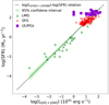 |
Fig. 4. Correlation between the [OI]63 μm and [OIII]88 μm summed emission line luminosities, in units of 1041 erg s−1, and the SFR derived from the total IR luminosity (black dashed line) for a composite sample of SFGs (red stars) and from the Hα luminosity (corrected for the IR luminosity) for LMG (green triangles). Purple squares indicate the sample of ULIRGs included in the SFG sample. |
3.2.4. Neon- and sulfur-based SFR tracers
A promising SFR tracer, proposed by Ho & Keto (2007), Zhuang et al. (2019), is the sum of the [NeII]12.8 μm and the [NeIII]15.6 μm emission line fluxes. By adding the two lines, this tracer is fairly independent of the effects related to the hardness of the radiation field, which are stronger at lower metallicities affecting single line diagnostics. For instance, while the [NeII]12.8 μm line intensity scales consistently in LMGs and SFGs, the [NeIII]15.6 μm line becomes remarkably brighter in LMGs (Fig. 1). Although some dependency on density is still expected, the high critical density of the sulphur (> 7 × 103 cm−3; see Table A.1) and the neon lines (> 5 × 104 cm−3) used in this section guarantees a minor effect on these tracers for the vast majority of the galaxy population.
In Fig. 3c, we show the correlation found between the summed luminosity of the [NeII] and [NeIII] emission lines and the SFR. This relation, obtained from data of 203 local SFGs, of which 182 are SFGs and 21 LMGs, can be expressed as follows:
![Mathematical equation: $$ \begin{aligned} \log \left(\frac{\mathrm{SFR}}{{M}_{\odot }\,\mathrm{yr}^{-1}}\right)=&(0.88 \pm 0.03)\nonumber \\&+(0.96 \pm 0.03) \log \left(\frac{L_{\rm [NeII]{+}[NeIII]}}{10^{41}\,\mathrm{erg\,s}^{-1}}\right), \end{aligned} $$](/articles/aa/full_html/2021/09/aa40696-21/aa40696-21-eq5.gif) (5)
(5)
where log(L[NeII]+[NeIII]) is the luminosity corresponding to the sum of the fluxes of the [NeII]12.8 μm and the [NeIII]15.6 μm lines. This relation has a Pearson coefficient of r = 0.91. In Fig. 3c, we report the comparison between the theoretical relation obtained by Zhuang et al. (2019) and our empirical one. The relation by Zhuang et al. (2019) is derived following the assumption that the neon lines trace all the ionising photons in a star forming region. Our relation, derived from observational data, shows a lower slope, and thus a larger offset, thus suggesting a lower efficiency in reprocessing the ionising photons by the neon transitions.
Analogously to the case of the two neon lines, we also take into consideration the sum of the two sulfur lines, [SIII]18.7 μm and [SIV]10.5 μm, as a tracer of the SFR. In Fig. 5a, we plot the correlation of the luminosity derived by summing [SIII]18.7 μm and [SIV]10.5 μm with the SFR derived from the total IR luminosity:
![Mathematical equation: $$ \begin{aligned} \log \left(\frac{\mathrm{SFR}}{{M}_{\odot }\,\mathrm{yr}^{-1}}\right)=&(1.07 \pm 0.06)\nonumber \\&+(1.04 \pm 0.05) \log \left(\frac{L_{\rm [SIII]{+}[SIV]}}{10^{41}\,\mathrm{erg\,s}^{-1}}\right)\cdot \end{aligned} $$](/articles/aa/full_html/2021/09/aa40696-21/aa40696-21-eq6.gif) (6)
(6)
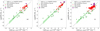 |
Fig. 5. a: correlation between the [SIV]10.5 μm and [SIII]18.7 μm summed emission line luminosity, expressed in units of 1041 erg s−1, and the SFR derived from the total IR luminosity (black dashed line) for a composite catalogue of SFGs (red star) and from the Hα luminosity (corrected for the IR luminosity) for LMGs (green triangles). The shaded green areas in the three plots indicate the 95% confidence interval. b: correlation between the [NeII]12.8 μm and [SIV]10.5 μm summed luminosities and the SFR derived from the total IR luminosity (black dashed line) for SFGs (red star) and from the Hα luminosity (corrected for the IR luminosity) for LMGs (green triangles). c: correlation between the [NeIII]15.6 μm and [SIII]18.7 μm summed emission lines and the SFR derived from the total IR luminosity (black dashed line) for SFG (red star) and from the Hα luminosity (corrected for the IR luminosity) for LMG (green triangles). In all three figures, the purple squares highlight the ULIRG population in the SFG sample. |
For this relation, we used 52 SFGs and 25 LMGs, obtaining a relation with a Pearson r coefficient of r = 0.90.
As shown in Table A.1, Ne+ has an ionisation potential (IP) of 21.56 eV, while Ne2+ has an IP of 40.96 eV and a potential of the next stage at 63.45 eV, thus covering the ∼20−60 eV energy interval. This is roughly the same ionisation interval covered by the [NeII]+[SIV], with [SIV] having an IP of 34.79 eV and the next stage IP being at 47.22 eV; or by [NeIII]+[SIII], with [SIII]18.7 μm having an IP of 23.34 eV. Analysing the former pair, we find the linear correlation between L[NeII]+[SIV] and SFR shown in Fig. 5b and expressed as follows:
![Mathematical equation: $$ \begin{aligned} \log \left(\frac{\mathrm{SFR}}{{M}_{\odot }\,\mathrm{yr}^{-1}}\right)=&(0.85 \pm 0.05)\nonumber \\&+(0.94 \pm 0.04) \log \left(\frac{L_{\rm [NeII]{+}[SIV]}}{10^{41}\,\mathrm{erg\,s}^{-1}}\right)\cdot \end{aligned} $$](/articles/aa/full_html/2021/09/aa40696-21/aa40696-21-eq7.gif) (7)
(7)
This relation has been calculated using 77 galaxies, of which 56 are SFGs and 21 are LMGs, and it has a Pearson correlation coefficient of r = 0.93. The small number of SFGs used to determine this relation is due to the lack of [SIV] measurements available in literature due to the intrinsic line faintness in SFGs (see Table D.1) and the position of the line in the silicate absorption band in the 9−11 μm range.
The relation between the SFR and the [NeIII]+[SIII] emission sum is shown in Fig. 5c and can be expressed as follows:
![Mathematical equation: $$ \begin{aligned} \log \left(\frac{\mathrm{SFR}}{{M}_{\odot }\,\mathrm{yr}^{-1}}\right)=&(1.16 \pm 0.04)\nonumber \\&+(1.03 \pm 0.04) \log \left(\frac{L_{\rm [NeIII]{+}[SIII]}}{10^{41}\,\mathrm{erg\,s}^{-1}}\right)\cdot \end{aligned} $$](/articles/aa/full_html/2021/09/aa40696-21/aa40696-21-eq8.gif) (8)
(8)
This relation has been calculated using 165 galaxies, of which 140 are SFGs and 25 are LMGs, and it has a Pearson correlation coefficient of r = 0.86.
3.2.5. PAH SFR tracer
In the mid-IR range, the emission features due to the PAH molecules arise from PDRs around H II regions embedding young stars (e.g. Draine & Li 2007) and can be used as SFR tracers. We analysed the PAH features at 6.2 and 11.3 μm, considering the same sample of 155 SFGs and the sample of 103 AGN galaxies described in Sect. 2 for the PAH analysis. As discussed in Sect. 3.1, we have not computed the correlation between the PAH and the IR luminosity in LMGs, and we therefore exclude LMGs from the SFR determination with the PAH.
The use of the PAH as a measure of the SFR was originally proposed by Wu et al. (2005), who used the Spitzer-IRAC camera (Fazio et al. 2004) 8 μm band of which the flux density is dominated by the strongest PAH feature (i.e. that at 7.7 μm). They derived a calibration of the 8 μm SFR using the radio VLA emission at 1.4 GHz and the Hα luminosity from the SFR-radio-luminosity relation given by Yun et al. (2001) and the SFR-Hα luminosity from Kennicutt (1998), respectively.
More recently, the relatively bright PAH features at 6.2, 7.7, and 11.3 μm have been used to derive a total PAH luminosity and have been correlated to the extinction-corrected Hα luminosity of a sample of 227 galaxies (Shipley et al. 2016). For SFGs (105 galaxies), the total PAH luminosity correlates linearly with the extinction-corrected Hα luminosity.
In Fig. 6, we show the correlation of the single PAH features and the SFR. Panel a shows the relation calculated for the 6.2 μm feature using 142 SFGs and 56 AGN, while panel b shows the relation for the 11.3 μm feature, for which we used 142 SFGs and 77 AGN. When computing these correlations, we excluded all ULIRGs from the original sample of AGN and SFGs, following the approach by Pope et al. (2013) to avoid saturation effects in the PAH-to-continuum luminosities. Moreover, when considering the AGN sample, we discarded all sources with a total IR luminosity greater than LIR = 1045 erg s−1, where the total IR luminosity, and therefore the derived SFR, could be severely contaminated by the AGN. Nevertheless, these are a few sources that do not affect the derived fit parameter when they are included in the fit. The two relations are described, respectively, by the following equations, which also report the Pearson r coefficient relative to each equation:
 (9)
(9)
 (10)
(10)
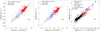 |
Fig. 6. a: correlation between the PAH emission feature at 6.2 μm, expressed in units of 1041 erg s−1 and the SFR derived from the total IR luminosity (black line) for a composite catalogue of SFGs (red star) and AGN-dominated galaxies (blue square). The shaded area in the three plots indicates the 95% confidence interval. b: correlation between the PAH emission feature at 11.3 μm, expressed in units of 1041 erg s−1 and the SFR derived from the total IR luminosity (black line) for a composite catalogue of SFGs (red star) and AGN-dominated galaxies (blue square). Panels a and b: we exclude ULIRGs from both AGN and SFG samples due to the known PAH deficit in these sources, as well as AGN with luminosities above 1045 erg s−1, which could dominate the IR continuum used to estimate the SFR. c: comparison of the relation between PAH total luminosity and SFR derived by Shipley et al. (2016) (black solid line) and using our sample (red dashed line). Red stars indicate SFG, purple squares indicate the ULIRG sub-sample included in the GOALS sample, and grey circles represent a sample of local galaxies used in Xie & Ho (2019). |
Both results show a shallow slope significantly lower than unity. This is a consequence of including the AGN sample. Considering only the SFG sample, the slopes would increase, becoming 0.87 for the PAH feature at 6.2 μm and 0.90 for the 11.3 μm feature. On the other hand, while we excluded all ULIRGs, including these objects does not result in a significant change in the slope, which in fact remains comparable within the errors. In particular, including the entire AGN and SFG samples for the PAH feature at 6.2 μm results in a slope of 0.81 ± 0.03, while for the PAH feature at 11.3 μm the slope would be 0.78 ± 0.03.
We compared our results with those proposed by Shipley et al. (2016); in order to properly determine the SFR using the Hα and 24 μm luminosities, as was done by these authors, we selected only the SFGs, excluding the AGN, resulting in a sample composed of 100 sources with the 6.2, 7.7, and 11.3 PAH features and the 24 μm and the Hα data. We find that our estimate of the SFR is higher by ∼0.25 dex than that derived by Shipley et al. (2016) and almost linear in slope (see Fig. 6c). We obtain:
 (11)
(11)
with a Pearson r coefficient of r = 0.66. While the slope of our result is comparable, within the error, to that obtained by Shipley et al. (2016), we attribute the difference in the intercept to the significant difference in sample characteristics. In particular, the disagreement arises when we extrapolate the results obtained by Shipley et al. (2016) for local galaxies. The sample used by Shipley et al. (2016) is in fact composed of galaxies with redshifts in the z ∼ 0.2 − 0.6 range, while our sample has a mean redshift of z ∼ 0.027. Moreover, while our sample is primarily composed of LIRGs and ULIRGs, the sample used by these authors is mainly constituted of galaxies in the LIR ∼ 109 − 1012 L⊙ interval. We additionally compared our derived relation to a sample of local SFGs described by Xie & Ho (2019), for which the SFR derived from Hα, corrected by the flux at 24 μm was available in the literature. This sample is composed of local galaxies and, while the bulk of these galaxies present a lower total PAH luminosity, it follows the same relation derived from the GOALS sample. This suggests that the difference observed between our result and the result by Shipley et al. (2016) is indeed due to an intrinsic difference of the sample used.
3.2.6. H2 SFR tracers
Molecular hydrogen is the most abundant molecule in the Universe and can be found in various environments. It can be excited by UV fluorescence (Black & van Dishoeck 1987), shocks (Hollenbach & McKee 1989), or X-ray illumination (Maloney 1997), thus probing various astrophysical environments. H2 forms on the surface of dust grains, affecting the ISM’s chemistry, and acts as a coolant. It is particularly important in all processes that regulate star formation and galaxy evolution, where the principal mechanism of these lines is associated with the UV radiation from massive stars.
Comparing theoretical models to observations, Rigopoulou et al. (2002) found evidence that an important fraction of H2 emission in SFGs can originate in PDRs. In this section, we test the use of different H2 molecular lines as SFR tracers. In Fig. 7a, we show the correlation between the H2 (S(3)) molecular line at 9.67 μm and the SFR determined from the total LIR for the SFG in the GOALS sample. We find a relation expressed by
 (12)
(12)
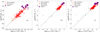 |
Fig. 7. a: correlation between the H2 molecular line at 9.67 μm, expressed in units of 1041 erg s−1, and the SFR derived from the total IR luminosity (black line) for a catalogue of SFGs (red star). b: correlation between the H2 molecular line at 12.28 μm, expressed in units of 1041 erg s−1, and the SFR derived from the total IR luminosity (black line) for a catalogue of SFGs (red star). The green triangle shows LMG detection, which was not used to derive the correlation. c: correlation between the H2 molecular line at 17.03 μm, expressed in units of 1041 erg s−1, and the SFR derived from the total IR luminosity (black line) for a catalogue of SFGs (red star). In all three figures, the shaded areas show the 95% confidence interval of the relations, and the purple squares highlight the ULIRG population in the SFG sample. |
which was determined using 168 SFGs, with a Pearson r coefficient of r = 0.87. Figure 7b shows the correlation between the H2 (S(2)) line at 12.28 μm and the SFR, determined with a sample of 126 SFGs and with a Pearson coefficient of r = 0.86 and expressed by
 (13)
(13)
Finally, Fig. 7c shows the correlation between the H2 (S(1)) line at 17.03 μm and the SFR, derived from a sample of 154 SFGs, with r = 0.85 and expressed by
 (14)
(14)
In Figs. 7b and c, we also report seven detections in LMGs of S(2) and S(1), respectively (shown in green). We did not include the LMG sample in the correlation due to the low number of sources, limiting ourselves to a comparison of the results. While a good correlation is lacking for the S(1) line, for the S(2) line we have a good agreement between the LMG population and the SFG one. This can be of particular interest in LMGs where the CO emission is considerably lower than what would correspond to the estimated SFR, implying the presence of CO-dark molecular gas that is not traced by the CO emission in LMGs (Togi & Smith 2016). We speculate that the sub-linear slopes obtained for the S(2) and S(3) lines might be linked to the different gas excitation temperature associated with each line. In particular, by moving to higher excitation lines and thus to shorter wavelengths, the H2 transitions are originated by an increasingly warmer gas in a thinner layer of the molecular gas clouds. Tracing the warmest material might cause the flattening of the slope since colder star-forming clouds are not detected by the higher transitions. Additionally, S(2) and S(3) lines could receive a more significant contribution from other excitation mechanisms, as suggested by the different excitation temperatures measured for these transitions in the Boltzmann diagrams for nearby galaxies (e.g. Tommasin et al. 2010).
We have not included the AGN sample in this section due to the different excitation mechanisms that can contribute to the H2 rotational lines in these sources, such as shocks or X-ray illumination. For the same reason, H2 lines are not used as BHAR tracers in Sect. 3.3 either, since they respond to the excitation temperature rather than the hardness of the ionising continuum. This makes it quite difficult to establish a clear connexion between the line intensities and the SFR or the accreted mass onto the black hole when both contributions are present.
3.3. BHAR tracers
The [OIV]25.9 μm and the [NeV]24.3 μm lines can be used to trace AGN activity. From our catalogue of AGN, derived from the 12 μm sample, we compiled the 2−10 keV X-ray fluxes from the literature, corrected for absorption. We then selected all objects with a hydrogen column density of NH ≤ 5 × 1023 cm−2 in order to exclude Compton-thick objects for which the 2−10 keV X-rays can be substantially absorbed, thus obtaining a sub-catalogue of 42 objects. For these objects, we investigated the correlation between the [OIV]25.9 μm line luminosity and the 2−10 keV X-ray luminosity (see Fig. 8a).
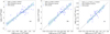 |
Fig. 8. a: linear correlation between the [OIV]25.9 μm and the 2−10 keV X-ray luminosity. b: linear correlation between the [NeV]24.3 μm line luminosity and the 2−10 keV X-ray luminosity. c: linear correlation between the [OIV]25.9 μm line luminosity and the 19 μm luminosity. All luminosities are expressed in units of 1041 erg s−1. |
We find a correlation expressed by the following equation:
![Mathematical equation: $$ \begin{aligned} \log \left(\frac{L_{\rm X}}{10^{41}\,\mathrm{erg\,s}^{-1}}\right)=&(1.85 \pm 0.07)\nonumber \\&+(1.21 \pm 0.10)\log \left(\frac{L_{\rm [OIV]25.9}}{10^{41}\,\mathrm{erg\,s}^{-1}}\right), \end{aligned} $$](/articles/aa/full_html/2021/09/aa40696-21/aa40696-21-eq15.gif) (15)
(15)
with a Pearson r coefficient of r = 0.87. In order to obtain a measure of the BHAR, it is necessary to convert the luminosity in the 2−10 keV band to the bolometric luminosity of the object, and from there to the BHAR (LAGN = ηṀBHc2). Different studies have been carried out to determine the best bolometric correction to apply when considering the 2−10 keV luminosity, with those by Marconi et al. (2004) and Lusso et al. (2012) being the most used in the literature. The resulting bolometric luminosities obtained applying these corrections are different, giving us a range of possible values. We applied both corrections to our data, and then from the resulting bolometric luminosities we calculated two linear relations linking the [OIV]25.9 μm line luminosity to the BHAR. Assuming a radiative efficiency of η = 0.1, in Eq. (16) we obtain the linear correlation applying the bolometric correction from Lusso et al. (2012), and in Eq. (17) the one applying the correction from Marconi et al. (2004). The equations are reported followed by their respective Pearson r coefficients:
![Mathematical equation: $$ \begin{aligned} \log \left(\frac{\dot{M}_{\rm BH}}{{M}_{\odot }\,\mathrm{yr}^{-1}}\right)=&(-1.65 \pm 0.07)+(1.04 \pm 0.09)\nonumber \\& \times \log \left(\frac{L_{\rm [OIV]25.9}}{10^{41}\,\mathrm{erg\,s}^{-1}}\right),\,\,r=0.86, \end{aligned} $$](/articles/aa/full_html/2021/09/aa40696-21/aa40696-21-eq16.gif) (16)
(16)
![Mathematical equation: $$ \begin{aligned} \log \left(\frac{\dot{M}_{\rm BH}}{{M}_{\odot }\,\mathrm{yr}^{-1}}\right)=&(-1.66 \pm 0.09)+(1.49 \pm 0.12)\nonumber \\& \times \log \left(\frac{L_{\rm [OIV]25.9}}{10^{41}\,\mathrm{erg\,s}^{-1}}\right),\,\,r=0.87. \end{aligned} $$](/articles/aa/full_html/2021/09/aa40696-21/aa40696-21-eq17.gif) (17)
(17)
In a similar way, we first calculated the linear correlation between the [NeV]24.3 μm line luminosity and the 2−10 keV luminosity (see right panel in Fig. 8). In this case, we have a total of 34 objects due to the smaller number of [NeV] data available, and we obtained a linear relation described by the following equation:
![Mathematical equation: $$ \begin{aligned} \log \left(\frac{L_{\rm X}}{10^{41}\,\mathrm{erg\,s}^{-1}}\right)=&(2.40 \pm 0.08)\nonumber \\&+(0.95 \pm 0.11)\log \left(\frac{L_{\rm [NeV]24.3}}{10^{41}\,\mathrm{erg\,s}^{-1}}\right), \end{aligned} $$](/articles/aa/full_html/2021/09/aa40696-21/aa40696-21-eq18.gif) (18)
(18)
with a Pearson coefficient of r = 0.84. We then applied the same bolometric corrections, obtaining linear correlations between the line luminosity and the BHAR, expressed by Eqs. (19) and (20) for the Lusso et al. (2012) and Marconi et al. (2004) corrections, respectively:
![Mathematical equation: $$ \begin{aligned} \log \left(\frac{\dot{M}_{\rm BH}}{{M}_{\odot }\,\mathrm{yr}^{-1}}\right)=&(-1.11 \pm 0.09)+(1.06 \pm 0.12)\nonumber \\& \times \log \left(\frac{L_{\rm [NeV]24.3}}{10^{41}\,\mathrm{erg\,s}^{-1}}\right),\,\,r=0.83, \end{aligned} $$](/articles/aa/full_html/2021/09/aa40696-21/aa40696-21-eq19.gif) (19)
(19)
![Mathematical equation: $$ \begin{aligned} \log \left(\frac{\dot{M}_{\rm BH}}{{M}_{\odot }\,\mathrm{yr}^{-1}}\right)=&(-0.89 \pm 0.11)+(1.47 \pm 0.15)\nonumber \\& \times \log \left(\frac{L_{\rm [NeV]24.3}}{10^{41}\,\mathrm{erg\,s}^{-1}}\right),\,\,r=0.84. \end{aligned} $$](/articles/aa/full_html/2021/09/aa40696-21/aa40696-21-eq20.gif) (20)
(20)
As a general trend, we find that both the [NeV]24.3 μm and [OIV]25.9 μm lines correlate linearly with the 2−10 keV X-ray luminosity, thus providing a good proxy to measure the AGN activity, as shown in Figs. 8a and b.
Following the work by Tommasin et al. (2010), we also analysed the correlation between the [NeV]24.3 and [OIV]25.9 μm lines with the luminosity at 19 μm. The luminosity at 19 μm (L19 μm) was used for two main reasons. On one hand, accurate Spitzer-IRS observations are available for the 19 μm flux density, from two different apertures, for the considered sample of galaxies. On the other hand, the 19 μm photometry data are the only available accurate photometric data closest to the emission at 12 μm. The 12 μm emission is, in turn, the best proxy for the bolometric flux of an active galaxy (Spinoglio et al. 1995). In particular, Tommasin et al. (2010) found that the 19 μm luminosity correlates with the [NeV]14.3 μm line luminosity.
The L19 μm was used by Tommasin et al. (2010) to compute the percentage of AGN and starburst components in 51 sources of their sample. Following these results, we selected all sources with an AGN component at 19 μm equal to or above 85%, and for this sub-sample of 35 objects we determined the correlation between the [OIV]25.9 μm and the [NeV]24.3 μm line luminosities with the 19 μm luminosity. These correlations are shown in Figs. 8c and 9a, respectively, and expressed by Eqs. (21) and (22), respectively, where r indicates the Pearson correlation coefficient, and n the number of objects used to derive the correlation:
![Mathematical equation: $$ \begin{aligned} \log \left(\frac{L_{19\,\upmu \mathrm{m}}}{10^{41}\,\mathrm{erg\,s}^{-1}}\right)=&(2.72 \pm 0.06)+(0.77 \pm 0.10)\nonumber \\& \times \log \left(\frac{L_{\rm [OIV]25.9}}{10^{41}\,\mathrm{erg\,s}^{-1}}\right),\,\,r=0.81,\,\,n=32, \end{aligned} $$](/articles/aa/full_html/2021/09/aa40696-21/aa40696-21-eq21.gif) (21)
(21)
![Mathematical equation: $$ \begin{aligned} \log \left(\frac{L_{19\,\upmu \mathrm{m}}}{10^{41}\,\mathrm{erg\,s}^{-1}}\right)=&(3.12 \pm 0.06)+(0.81 \pm 0.10)\nonumber \\& \times \log \left(\frac{L_{\rm [NeV]24.3}}{10^{41}\,\mathrm{erg\,s}^{-1}}\right),\,\,r=0.85,\,\,n=30. \end{aligned} $$](/articles/aa/full_html/2021/09/aa40696-21/aa40696-21-eq22.gif) (22)
(22)
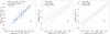 |
Fig. 9. a: linear correlation between the [NeV]24.3 μm line luminosity and the 19 μm luminosity, expressed in units of 1041 erg s−1. b: comparison of the three different relations between the [OIV]25.9 μm line luminosity and the BHAR: the blue dashed line reports the relation obtained from the Lusso et al. (2012) bolometric correction, the red dotted line the relation from the Marconi et al. (2004) bolometric correction, and the green solid line the results from the Spinoglio et al. (1995) correction. c: same as panel a, but for the [NeV]24.3 μm line. |
We then used these relations, (Eqs. (21) and (22)) to determine the bolometric luminosity of our sources and the accretion rate. In order to calculate the bolometric luminosity, we used the relation calculated by Spinoglio et al. (1995) that links the bolometric luminosity to the 12 μm luminosity. The 12 μm luminosity for our sample was determined using data from Deo et al. (2009): the authors report continuum measurements at 5.5 μm, 14.7 μm, and 20 μm taken from Spitzer low-resolution spectroscopic observations. Where possible, we interpolated the continuum slope and the 12 μm continuum flux using the 5.5 μm and 14.7 μm measurements, otherwise (but only in three cases) using the extrapolation from the 14.7 μm and 20 μm fluxes. We then matched the Deo et al. (2009) sample with the Tommasin et al. (2010) sample and calculated the bolometric luminosity starting from the monochromatic 12 μm luminosity for those sources with a 85% AGN component. Similarly to what was done for the 2−10 keV luminosity, we determined the BHAR, starting from the bolometric luminosity derived from the 12 μm luminosity, and its relation to the [NeV]24.3 μm and [OIV]25.9 μm line luminosities, obtaining the following relations:
![Mathematical equation: $$ \begin{aligned} \log \left(\frac{\dot{M}_{\rm BH}}{{M}_{\odot }\,\mathrm{yr}^{-1}}\right)=&(-1.14 \pm 0.07)+(0.67 \pm 0.15)\nonumber \\& \times \log \left(\frac{L_{\rm [OIV]25.9}}{10^{41}\,\mathrm{erg\,s}^{-1}}\right),\,\,r=0.68,\,\,n=26, \end{aligned} $$](/articles/aa/full_html/2021/09/aa40696-21/aa40696-21-eq23.gif) (23)
(23)
![Mathematical equation: $$ \begin{aligned} \log \left(\frac{\dot{M}_{\rm BH}}{{M}_{\odot }\,\mathrm{yr}^{-1}}\right)=&(-0.77 \pm 0.10)+(0.77 \pm 0.16)\nonumber \\& \times \log \left(\frac{L_{\rm [NeV]24.3}}{10^{41}\,\mathrm{erg\,s}^{-1}}\right),\,\,r=0.71,\,\,n=24. \end{aligned} $$](/articles/aa/full_html/2021/09/aa40696-21/aa40696-21-eq24.gif) (24)
(24)
The smaller number of objects used to derive these relations is due to the lack of data for the determination of the continuum at 12 μm.
Measuring the BHAR requires important approximations in terms of bolometric correction, which can yield significantly different results. Between the three proposed bolometric corrections, we note that the correlations obtained when applying the Marconi correction are steeper than those obtained from the Lusso and Spinoglio corrections. In particular, we compare the results in Fig. 9; for both the [OIV]25.9 μm (panel b, at the centre) and [NeV]24.3 μm (panel c, on the right) lines, we note that the results derived from the corrections of Spinoglio et al. (1995) and Lusso et al. (2012) show a similar, flatter slope, indicating, within the errors, the expected linear relation between the line tracers and the BHAR. It is important to note that the Marconi et al. (2004) and Lusso et al. (2012) bolometric corrections are based on a third-degree polynomial transformation of the X-ray luminosity. This necessarily leads to deviations from the slopes obtained in Eqs. (15) and (18).
We refer the reader to Appendix C for a discussion on the use of the mid-ionisation lines of [NeIII]15.5 μm and [SIV]10.5 μm as alternative BHAR tracers.
4. Discussion
4.1. Applicability of our results to composite objects
The coexistence of AGN and star formation in galaxies is well known (see, e.g. Pérez-Torres et al. 2021, for a review) and therefore we expect many galaxies to be characterised by both components at work together. In general, when considering composite objects, with both an SF and an AGN component detectable, our results in Sects. 3.2 and 3.3 can still be applied.
We used the GOALS sample to determine whether the results on the SFR tracers can be applied to composite objects (Sect. 3.2). The GOALS sample is composed of SFG, but for part of the sample an AGN component is also present, if not always detected. For our calibrations, we excluded all sources for which a [NeV] emission line is detected. Here, we instead include all objects of the sample. In Fig. 10, we plot the ratio of the SFR obtained using the [NeII]+[NeIII] tracer to the SFR obtained using the 11.3 μm PAH feature, as a function of the equivalent width (EW) of the PAH feature at 6.2 μm, as determined by Stierwalt et al. (2014). The mean ratio for the entire population is −0.049, with the median value equal to −0.023 and 50% of the sample included in the [−0.18, 0.06] interval. While there is some dispersion around zero, for the majority of the sample we obtain a similar SFR whether we use the [NeII]+[NeIII] tracer or the PAH tracer. This suggests that for mixed objects these two tracers are equivalent, and independent of the presence of an AGN. Significant differences are observable for the extreme objects in the sample: the sources with the larger AGN content are located in the top left corner, and the SFR obtained using the [NeII]+[NeIII] tracer is significantly higher than the SFR obtained using the PAH. This is plausibly due to an increase in the [NeIII] emission related to the presence of the AGN.
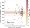 |
Fig. 10. Comparison of the ratio between the SFR obtained using the [NeII]+[NeIII] tracer and the SFR obtained using the PAH feature at 11.3 μm against the EW of the PAH feature at 6.2 μm for the GOALS sample. The colour gradient indicates the percentage of the AGN component in each object as determined by mid-IR tracers (Díaz-Santos et al. 2017). The black dashed line shows the mean value of the SFR ratio for the population, with the shaded area indicating where the 50% of the entire sample is located. The red dotted lines represent the 1σ interval around the mean value. |
4.2. Comparing the various tracers
Summarising the results presented in Sect. 3.2, among the various SFR tracers presented, for galaxies dominated by SF processes we suggest that the best tracers are the [CII]158 μm line (slope α = 0.89 ± 0.02 and correlation coefficient r = 0.92) or the combination of the [OI] and [OIII] lines (slope α = 1.25 ± 0.04 and r = 0.94) for high-redshift galaxies observed from the ground with sub-millimetre telescopes. For galaxies observed from space or airborne facilities (but also from the new generation of the very large optical ground-based telescopes in the 8−13 μm atmospheric window, for local galaxies), the best SFR tracers are the combination of the [NeII] and [NeIII] lines (slope α = 0.96 ± 0.03 and r = 0.91) or the combination of the other mid-IR fine-structure lines. For galaxies containing an AGN, the PAH features can reliably be used, and the PAH 11.3 μm feature is probably the best SFR tracer (slope α = 0.75 ± 0.04 and r = 0.79). As an alternative, the [NeII] and [NeIII] lines can also still be used in AGN with the correction to the total neon flux that can be computed using one of the [NeV] lines, as suggested by Zhuang et al. (2019).
When measuring the BHAR, following the results presented in Sect. 3.3, the [NeV] lines at 14.3 and 24.3 μm are exclusive probes of AGN activity, because their emission is a direct signature of the hard ionising spectrum due to the accretion process. However, these lines are fainter than the [OIV]25.9 μm line, which can be detected more easily in faint objects. When using the [OIV] line as a BHAR tracer, it is important to take account of the possible contamination due to SF processes, because its emission can also be attributed, to some extent, to starburst activity (Lutz et al. 1998).
4.3. Comparison with previous line calibrations
We briefly compare the results of the line calibrations obtained in this work with those of Spinoglio et al. (2012, 2014) and Gruppioni et al. (2016). The details of the comparisons can be found in Appendix E. We note that in this work, to derive the correlations we used the orthogonal distance regression method, instead of the least-squares minimisation method, which was used by the other authors, because we consider the total IR luminosity and the line luminosity to be two independent variables.
The AGN sample used in this work and in Spinoglio et al. (2012) is the same for the lines in the 10−35 μm interval, and the differences in the correlation are only due to the different methods of analysis. We note that in this work, in order to obtain a correlation between the total LIR and the [OIV]25.9 μm line luminosity that better represents the AGN population, we did not use the entire sample of AGNs by Tommasin et al. (2008, 2010), but a sub-sample of objects with an AGN component in the 19 μm luminosity of at least 85% (see Sect. 3.1).
For the SFG sample, while in Spinoglio et al. (2012) the sample of galaxies described by Bernard-Salas et al. (2009) was used, in this work we expanded the same sample by including the LIRG and ULIRG GOALS samples, as described in Sect. 2. Nonetheless, we obtain comparable results, except in the cases of the PAH feature at 11.3 μm and of the H2 line at 17.03 μm, for which our results show line luminosities an order of magnitude higher. This is due to the presence, in our sample, of LIRGs and ULIRGs, which shift the relation towards a steeper slope.
For the lines at wavelengths in the 50−158 μm range, we refer the reader to Appendix E, where we discuss the differences and plot the results of the different calibrations of Spinoglio et al. (2012) with respect to our results.
Because of the different analytical method used to determine the correlations between the total and line luminosities, for the comparison with Spinoglio et al. (2012) we recomputed our calibrations using the least-squares fit and give the results in Appendix E. For the comparison with Gruppioni et al. (2016), we instead recomputed the correlations of the Gruppioni et al. (2016) sample, applied the orthogonal distance regression, and then compared these with our results. As a general trend, we find good agreement between our results and those of Gruppioni et al. (2016), with comparable slopes within 2σ of each other. For all the details and the plots of the results of the different calibrations, we refer the reader to Appendix E.
We do not compare our results with those obtained by Bonato et al. (2019), since the methods of analysis are widely different. In particular, while in this work we calibrated the line luminosities leaving the slope of the correlations as a free parameter, in Bonato et al. (2019) the slope of the relation was fixed to unity, thus giving raise to substantial differences in the results.
4.4. Metallicity and SFR tracers
In Sect. 3.2.2, we revise the [CII]–SFR relation for a wide galaxy sample, from LMGs to extreme ULIRGs. In Sect. 3.2.4, we derive a measure of the SFR through the neon and sulfur mid-IR lines and propose new SFR tracers using different combinations of these lines. In this section, we discuss the possible effects that metallicity, and the associated changes in the ISM of these galaxies, may have on these tracers.
First of all, for the sample of dwarf galaxies, we adopted SFR values derived from the observed Hα luminosity and corrected from the total IR luminosity (Rémy-Ruyer et al. 2015). This is motivated by the underestimation of the SFR by the IR luminosity at very low metallicities (12 + log(O/H)≲8.5; Lee et al. 2013) due to the lower metal abundance in these galaxies compared to SFGs. In principle, the lower dust-to-gas ratio of an LMG should also have an impact on the observed intensities of the fine-structure lines. This is, however, balanced by the higher cooling rates in these transitions, as discussed by De Looze et al. (2014).
Figure 3a shows that the [CII]158 μm emission in LMGs follows the trend found in SFGs, with no need to perform any additional correction for metallicity in these galaxies. Similarly, the different combinations of [NeII]12.8 μm, [NeIII]15.6 μm, [SIII]18.7 μm, and [SIV]10.5 μm, shown in Figs. 3 and 5, follow the correlation of solar-like metallicity galaxies. The higher cooling rates in LMG are particularly evident when the neon and sulfur transitions are considered. While the [NeII]12.8 μm emission in LMGs scales with LIR similarly to SFGs (Fig. 1b), the [NeIII]15.6 μm line becomes comparatively much brighter for a given IR luminosity, more than one order of magnitude above the correlation found for SFG, as can also be seen by the value of the constant b in the best-fit equation for the [NeIII]15.6 μm line in Table A.1. When considering the sulfur lines, this effect is even more pronounced (see Fig. B.4a and Table A.1). This means that mid- to high-ionisation species such as Ne2+ or S3+ trace a contribution to the star formation that is not revealed either by the Ne+ and S2+ low-ionisation gas or the IR emission. Thus, the combination of low- and high-ionisation lines allows us to trace the total star formation in both low- and solar-metallicity galaxies (Ho & Keto 2007; Zhuang et al. 2019).
In the case of the [CII]158 μm line, Fig. 3a suggests that this transition remains a dominant coolant of the ISM at low metallicities. Given its low-ionisation potential (11.3 eV, see Table A.1), this line can originate from both neutral and ionised gas, and one could expect a decreasing contribution from the neutral component as the ionisation field becomes harder at low metallicities. However, Cormier et al. (2019) demonstrated that the PDR contribution to the global [CII]158 μm emission is still dominant for the same LMG sample used in this work. This is also in line with the results of Croxall et al. (2017), suggesting that the [CII]158 μm emission linked to ionised gas is of the order of ∼10% in LMG, and up to a maximum of < 40% where a high U is required. Moreover, analytical models developed in these studies show a decrease of [CII] emission from ionised gas with decreasing metallicity, with ∼55 − 75% of the [CII] emission arising from PDRs in LMGs and reaching almost 100% when the metallicity decreases below 1/4 Z⊙. Additionally, the thickness of the [CII] layer increases for molecular clouds exposed to the harder radiation fields typical of LMGs. This is shown by the detection of higher [CII]/CO(1−0) ratios in local LMGs when compared to SFG with solar or super-solar metallicity (e.g. Madden et al. 1997; Madden 2000; Hunter et al. 2001), and this is supported by PDR models (Bolatto et al. 1999; Röllig et al. 2006).
While a detailed study of the ionised gas and PDR structure is out of the scope of the present work, the results discussed above suggest that both [CII]158 μm and the different combinations of neon and sulphur lines are robust star formation tracers, virtually independent of dust extinction, which can be applied to a wide diversity of environments with different physical conditions and metallicities. Specifically, the variations expected from the changes in the chemical abundances are mostly balanced by the increase in the cooling rates of these transitions.
4.5. Comparison with high-z data
We compare the calibrations described in Sect. 3.1 obtained for local galaxies to high-redshift detections of sources obtained with ALMA. In particular, we consider detections of the [OIII]88 μm, [NII]122 μm, [CII]158 μm, and [NII]205 μm lines at z ≥ 3. Sources identified as QSOs are compared to local AGN results, while sources for which a classification is not given in the literature, or that are classified as starburst galaxies, are compared to local SFGs.
Figure 11a shows the comparison between local and high-redshift detections of the [CII]158 μm line for QSO galaxies, and in particular 27 detections at z ∼ 6 reported in Venemans et al. (2020), plus the detections by Walter et al. (2018) for one source at z ∼ 6.08 and by Hashimoto et al. (2019) for two sources at z ∼ 7.1, for a total of 30 sources. Figure 11b displays the comparison of local and high-redshift SFGs: 84 detections from the ALPINE catalogue (Faisst et al. 2020), plus nine other detections (Inoue et al. 2016; Vishwas et al. 2018; Walter et al. 2018; De Breuck et al. 2019; Hashimoto 2019; Harikane et al. 2020; Rybak et al. 2020), for a total of 93 objects with redshift in the 4.2 ≲ z ≲ 7.2 range. While some outliers are present, the bulk of the detections in both cases lies within the prediction interval, which we show in the figures at the 95% level, suggesting that the relations derived for local galaxies hold for high-redshift sources.
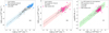 |
Fig. 11. a: comparison between the LIR–L[CII]158 relation (black dashed line) for local AGN dominated galaxies (grey squares) and high-redshift detections for QSOs (blue symbols). The shaded area shows the 95% prediction interval. b: same for high-redshift starburst galaxies (pink symbols). c: comparison of the local log(L[CII]–log(SFR) relation (black dashed line) and L[CII]–SFR values of high-redshift sources (pink symbols). Grey dots represent local SFGs. The shaded area shows the 95% prediction interval for the local relation. |
In Fig. 11c, we compare the L[CII]–SFR relation extrapolated for local galaxies (see Sect. 3.2.2) with ALPINE detections of the [CII]158 μm emission line in starburst galaxies. We find that high-redshift objects follow the same L[CII]–SFR relation as local SFGs and LMGs, thus suggesting little or no evolution in the L[CII]–SFR relation. In particular, no deficit of [CII] emission is seen for the highest SFR values of ∼100 M⊙ yr−1, suggesting that starbursts at high z might not behave like local ULIRGs such as those shown in Fig. 3 (purple squares). An analogous result was found by Schaerer et al. (2020), who analysed a large sample of galaxies at high redshift (z ∼ 4 − 6) observed by ALMA. Leung et al. (2020) explored the possibility of tracing the SFR at the epoch of recombination with [CII]158 μm using simulated data. Although they find a good correlation, when compared to observed data, the simulated sample shows an average [CII] luminosity lower than the one obtained from ALMA pointed observations. A similar result was obtained for simulations of high-redshift systems (Ferrara et al. 2019) showing the presence of under-luminous [CII] emission.
In Fig. 12a, we show the comparison between the local LIR–L[OIII]88 relation for AGN and high-redshift detections in QSOs (Hashimoto et al. 2019; Walter et al. 2018), while panel b shows the relation between local and high-redshift SFGs (Inoue et al. 2016; Vishwas et al. 2018; Walter et al. 2018; De Breuck et al. 2019; Harikane et al. 2020; Hashimoto 2019; Tamura et al. 2019). We note that while the high-redshift detections of [OIII]88 μm in QSOs are comparable with the relation derived from local AGN-dominated galaxies, in SFG the majority of high-redshift detections appear to be one to two orders of magnitude brighter at comparable LIR. These detections are better represented by the LIR–L[OIII]88 relation derived for local LMG (see Fig. 12b). This suggests that the [OIII]88 μm line is produced in an environment with a higher ionising spectrum, similar to the ISM of local LMGs (see Sect. 3.1).
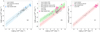 |
Fig. 12. a: comparison between the LIR–L[OIII]88 relation (black dashed line) for local AGN-dominated galaxies (grey squares) and high-redshift detections for QSOs (blue symbols). b: comparison between the LIR–L[OIII]88 relation (red dashed line) for local SFG (grey stars) and high-redshift detections for starburst galaxies (pink symbols). The red shaded area shows the 95% prediction interval of this relation. For comparison, the green dashed line shows the LIR–L[OIII]88 relation for local LMG, with grey squares indicating local LMGs and the green shaded area giving the 95% prediction interval for this relation. c: comparison of the local LIR–L[NII]205 relation (black dashed line) for high-redshift detections of SFGs (pink symbols). Grey stars represent local SFGs. The shaded area in each figure shows the 95% prediction interval for the local relation. |
Finally, the high-redshift detections in panel c show the local LIR–L[NII]205 relation for SFGs and 17 high-redshift detections of [NII]205 μm (Cunningham et al. 2020), with the local correlation that also represents the high-redshift detections well. In Fig. B.8, we report the comparison between the local LIR–L[NII]122 relation and high-redshift SFGs: in this case only one object (De Breuck et al. 2019) was detected, while three (Harikane et al. 2020) objects have upper limits. Thus, only one object is located almost an order of magnitude higher than the local relation for SFGs, and therefore there is no statistical evidence of a difference in the production mechanism of [NII] in high-redshift objects, especially considering the results for the [NII]205 μm line.
4.6. Application to present and future facilities
The lines and features presented in this work can be observed in galaxies by present and future IR and sub-millimetre facilities. The JWST will be the next NASA observatory to explore the Universe in the near- and mid-IR spectral range. In particular, the JWST Mid-InfraRed Instrument (MIRI, Rieke et al. 2015; Wright et al. 2015) will be able to obtain imaging and spectra with unprecedented sensitivity in the 4.9 − 28.9 μm spectral range. In Fig. 13a, we compare the MIRI wavelength interval to the observability of key mid-IR lines at various redshifts. In particular, from the analysis presented in Sect. 3.2, it will be possible to study the SFR up to redshift z ∼ 3.5 with the PAH feature at 6.2 μm, up to redshift z ∼ 1.5 with the PAH feature at 11.3 μm, or up to z ∼ 0.8 using combinations of the neon and sulfur lines.
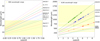 |
Fig. 13. Left: observability of key mid-IR (dashed lines) lines compared to the JWST-MIRI instrument (shaded area) in the 0−1.6 redshift interval. Right: observability of key far-IR (dashed lines) lines compared to the ALMA bands (shaded area) in the 1−8 redshift interval. Dots represent current detection for each line. |
On the other hand, while we do not report the [NeV]24.3 and [OIV]25.9 μm lines in Fig. 13a due to the limited wavelength range available for JWST, we show the [NeV]14.3 μm line, for which the same analysis carried out in Sect. 3.3 to derive the BHAR is applied and reported in Appendix C. The [NeV]14.3 μm line will be observed by the JWST-MIRI up to redshift z ≲ 1, while the [NeV]24.3 μm line will be observed up to redshift z ≲ 0.15, and the [OIV]25.9 μm line will be observed up to redshift z ≲ 0.1.
While the JWST-MIRI will be able to observe molecular and atomic lines up to redshift z ∼ 2, and the PAH up to higher redshift (z ∼ 3.5 for the 6.2 μm feature), ALMA is able to trace the far-IR lines, such as [CII]158 μm, up to redshift z ∼ 8, as shown in Fig. 13b, providing important information on the evolution of galaxies with cosmic time. An analogue study can be found in Fig. 1 of Carilli & Walter (2013), where the CO transitions and other key tracers of the ISM are shown as a function of redshift versus frequency in terms of the observability by ALMA and JVLA (Karl J. Jansky Very Large Array, Perley et al. 2011). We also report the redshift of the currently available data of ALMA detections in Fig. 13b: while lines like [CII]158 μm or [NII]205 μm are detected over a significant redshift interval, shorter wavelength lines such as [OI]63 μm present very few results. This is due to the difficulty of observing in the bands at a higher frequency, for which the atmospheric absorption allows good visibility for only 10% of the total observational time.
In the near future, the extremely large ground-based telescopes under construction, with dedicated instruments for N-band spectroscopy, will be able to obtain observations of the mid-IR spectral range 8−13 μm and thus will test the [SIV]10.5 μm + [NeII]12.8 μm relation, for local galaxies and AGN. The ESO Extremely Large telescope (E-ELT; Gilmozzi & Spyromilio 2007) is expected to obtain first light at the end of 2025, with the mid-IR ELT Imager and Spectrograph (METIS, Brandl et al. 2021) instrument covering the N band with imaging and low-resolution spectroscopy, and the Thirty Meter Telescope (TMT; Schöck et al. 2009) will have completed first light and will be ready for science operations at the end of 2027, and the Giant Magellan Telescope (GMT; Johns et al. 2012) will be operational in 2029.
5. Summary and conclusions
In this work, we systematically revise the calibration of lines and features in the 6−205 μm spectral range. We report new line-to-LIR calibrations for three galaxy types: AGN, LMGs, and SFGs, building well-defined samples with available IR spectroscopy mainly obtained from Herschel and Spitzer. The main results of this work are:
-
Statistically robust calibrations to the total IR luminosity were obtained for the bright IR lines and features, including the PAH features, the H2 pure rotational lines, and the fine-structure lines, mostly for all three galaxy populations, excluding the PAH features for the LMG and the high-ionisation fine-structure lines for the SFGs and LMGs.
-
The [CII]158 μm line can be used as an SFR tracer for both LMGs and SFGs, covering 6 orders of magnitude in luminosity, independently of the source metallicity. Moreover, when compared to high-redshift detections, the correlation obtained for local galaxies can still be applied.
-
The sum of the two far-IR oxygen lines, the [OI]63 μm line and the [OIII]88 μm line, can be used as a tracer for the SFR.
-
A combination of low- and intermediate-ionisation lines from neon and/or sulfur is also a robust proxy for the SFR, independent of the metallicity. In particular, the [SIV]10.5 μm + [NeII]12.8 μm tracer will be accessible to ELT facilities in the near future for galaxies in the local Universe.
-
The brightest PAH features at 6.2 and 11.3 μm can be reliably used for SFR tracers in both SFGs and AGN, while the lack of these features prevents their use in LMGs.
-
We present for the first time a correlation between the SFR and the H2 molecular line fluxes at 9.7, 12.3, and 17.0 μm.
-
The [CII]158 μm line, the combination of the two neon lines ([NeII]12.8 μm and [NeIII]15.5 μm), and, for solar-like metallicity galaxies that may harbour an AGN, the PAH 11.3 μm feature are the best SFR tracers.
-
The [NeV]14.3 μm, [NeV]24.3 μm and [OIV]25.9 μm lines are good tracers of the BHAR, derived either from the 2−10 keV luminosity or from the 12 μm luminosity.
These results are particularly relevant to the upcoming launch of the JWST, which will observe many of the mid-IR features with the MIRI instrument in galaxies of the local Universe and beyond, up to a redshift of ∼1 for the brightest lines, thus allowing us to measure both the SFR and the BHAR with spectroscopy.
Acknowledgments
We thank the anonymous referee for his/her comments which helped to improve the present article. LS and JAFO acknowledge financial support by the Agenzia Spaziale Italiana (ASI) under the research contract 2018-31-HH.0.
References
- Allamandola, L. J., Tielens, A. G. G. M., & Barker, J. R. 1989, ApJS, 71, 733 [Google Scholar]
- Armus, L., Charmandaris, V., Bernard-Salas, J., et al. 2007, ApJ, 656, 148 [NASA ADS] [CrossRef] [Google Scholar]
- Armus, L., Mazzarella, J. M., Evans, A. S., et al. 2009, PASP, 121, 559 [Google Scholar]
- Bernard-Salas, J., Spoon, H. W. W., Charmandaris, V., et al. 2009, ApJS, 184, 230 [Google Scholar]
- Berta, S., Lutz, D., Santini, P., et al. 2013, A&A, 551, A100 [NASA ADS] [CrossRef] [EDP Sciences] [Google Scholar]
- Black, J. H., & van Dishoeck, E. F. 1987, ApJ, 322, 412 [NASA ADS] [CrossRef] [Google Scholar]
- Boggs, P. T., & Rogers, J. E. 1990, in Orthogonal Distance Regression (Providence: American Mathematical Society), Contemp. Math., 112, 186 [Google Scholar]
- Bolatto, A. D., Jackson, J. M., & Ingalls, J. G. 1999, ApJ, 513, 275 [NASA ADS] [CrossRef] [Google Scholar]
- Bonato, M., De Zotti, G., Leisawitz, D., et al. 2019, PASA, 36, e017 [NASA ADS] [CrossRef] [Google Scholar]
- Brandl, B. R., Bernard-Salas, J., Spoon, H. W. W., et al. 2006, ApJ, 653, 1129 [NASA ADS] [CrossRef] [Google Scholar]
- Brandl, B., Bettonvil, F., van Boekel, R., et al. 2021, The Messenger, 182, 22 [NASA ADS] [Google Scholar]
- Buchanan, C. L., Gallimore, J. F., O’Dea, C. P., et al. 2006, AJ, 132, 401 [NASA ADS] [CrossRef] [Google Scholar]
- Bullock, J. S., & Boylan-Kolchin, M. 2017, ARA&A, 55, 343 [NASA ADS] [CrossRef] [Google Scholar]
- Calzetti, D., Kennicutt, R. C., Engelbracht, C. W., et al. 2007, ApJ, 666, 870 [NASA ADS] [CrossRef] [Google Scholar]
- Carilli, C. L., & Walter, F. 2013, ARA&A, 51, 105 [NASA ADS] [CrossRef] [EDP Sciences] [Google Scholar]
- Carpenter, J., Iono, D., Kemper, F., & Wootten, A. 2020, ArXiv e-prints [arXiv:2001.11076] [Google Scholar]
- Clegg, P. E., Ade, P. A. R., Armand, C., et al. 1996, A&A, 315, L38 [NASA ADS] [Google Scholar]
- Cormier, D., Lebouteiller, V., Madden, S. C., et al. 2012, A&A, 548, A20 [NASA ADS] [CrossRef] [EDP Sciences] [Google Scholar]
- Cormier, D., Madden, S. C., Lebouteiller, V., et al. 2015, A&A, 578, A53 [NASA ADS] [CrossRef] [EDP Sciences] [Google Scholar]
- Cormier, D., Abel, N. P., Hony, S., et al. 2019, A&A, 626, A23 [NASA ADS] [CrossRef] [EDP Sciences] [Google Scholar]
- Cortese, L., Boissier, S., Boselli, A., et al. 2012, A&A, 544, A101 [NASA ADS] [CrossRef] [EDP Sciences] [Google Scholar]
- Croxall, K. V., Smith, J. D., Pellegrini, E., et al. 2017, ApJ, 845, 96 [NASA ADS] [CrossRef] [Google Scholar]
- Cunningham, D. J. M., Chapman, S. C., Aravena, M., et al. 2020, MNRAS, 494, 4090 [NASA ADS] [CrossRef] [Google Scholar]
- Dale, D. A., Helou, G., Brauher, J. R., et al. 2004, ApJ, 604, 565 [NASA ADS] [CrossRef] [EDP Sciences] [Google Scholar]
- De Breuck, C., Weiss, A., Bethermin, M., et al. 2019, A&A, 631, A167 [NASA ADS] [CrossRef] [EDP Sciences] [Google Scholar]
- de Graauw, T., Haser, L. N., Beintema, D. A., et al. 1996, A&A, 315, L49 [NASA ADS] [Google Scholar]
- De Looze, I., Cormier, D., Lebouteiller, V., et al. 2014, A&A, 568, A62 [NASA ADS] [CrossRef] [EDP Sciences] [Google Scholar]
- Deo, R. P., Richards, G. T., Crenshaw, D. M., & Kraemer, S. B. 2009, ApJ, 705, 14 [NASA ADS] [CrossRef] [Google Scholar]
- Díaz-Santos, T., Armus, L., Charmandaris, V., et al. 2017, ApJ, 846, 32 [Google Scholar]
- Draine, B. T., & Li, A. 2007, ApJ, 657, 810 [NASA ADS] [CrossRef] [Google Scholar]
- Engelbracht, C. W., Gordon, K. D., Rieke, G. H., et al. 2005, ApJ, 628, L29 [NASA ADS] [CrossRef] [Google Scholar]
- Engelbracht, C. W., Rieke, G. H., Gordon, K. D., et al. 2008, ApJ, 678, 804 [NASA ADS] [CrossRef] [Google Scholar]
- Faisst, A. L., Schaerer, D., Lemaux, B. C., et al. 2020, ApJS, 247, 61 [NASA ADS] [CrossRef] [Google Scholar]
- Farrah, D., Lebouteiller, V., Spoon, H. W. W., et al. 2013, ApJ, 776, 38 [Google Scholar]
- Fazio, G. G., Hora, J. L., Allen, L. E., et al. 2004, ApJS, 154, 10 [NASA ADS] [CrossRef] [Google Scholar]
- Fernández-Ontiveros, J. A., Spinoglio, L., Pereira-Santaella, M., et al. 2016, ApJS, 226, 19 [NASA ADS] [CrossRef] [Google Scholar]
- Ferrara, A., Vallini, L., Pallottini, A., et al. 2019, MNRAS, 489, 1 [NASA ADS] [CrossRef] [Google Scholar]
- Förster Schreiber, N. M., & Wuyts, S. 2020, ARA&A, 58, 661 [Google Scholar]
- Galliano, F., Nersesian, A., Bianchi, S., et al. 2021, A&A, 649, A18 [EDP Sciences] [Google Scholar]
- Gardner, J. P., Mather, J. C., Clampin, M., et al. 2006, Space Sci. Rev., 123, 485 [Google Scholar]
- Gilmozzi, R., & Spyromilio, J. 2007, The Messenger, 127, 11 [Google Scholar]
- Goldsmith, P. F., Langer, W. D., Pineda, J. L., & Velusamy, T. 2012, ApJS, 203, 13 [Google Scholar]
- Goulding, A. D., & Alexander, D. M. 2009, MNRAS, 398, 1165 [NASA ADS] [CrossRef] [Google Scholar]
- Greenhouse, M. A., Feldman, U., Smith, H. A., et al. 1993, ApJS, 88, 23 [NASA ADS] [CrossRef] [Google Scholar]
- Gruppioni, C., Berta, S., Spinoglio, L., et al. 2016, MNRAS, 458, 4297 [Google Scholar]
- Harikane, Y., Ouchi, M., Inoue, A. K., et al. 2020, ApJ, 896, 93 [Google Scholar]
- Hashimoto, T. 2019, Am. Astron. Soc. Meet. Abstr., 233, 106.05 [NASA ADS] [Google Scholar]
- Hashimoto, T., Inoue, A. K., Tamura, Y., et al. 2019, PASJ, 71, 109 [NASA ADS] [CrossRef] [Google Scholar]
- Herrera-Camus, R., Bolatto, A. D., Wolfire, M. G., et al. 2015, ApJ, 800, 1 [Google Scholar]
- Ho, L. C., & Keto, E. 2007, ApJ, 658, 314 [NASA ADS] [CrossRef] [Google Scholar]
- Hollenbach, D., & McKee, C. F. 1989, ApJ, 342, 306 [NASA ADS] [CrossRef] [Google Scholar]
- Houck, J. R., Roellig, T. L., van Cleve, J., et al. 2004, ApJS, 154, 18 [NASA ADS] [CrossRef] [Google Scholar]
- Hunter, D. A., Kaufman, M., Hollenbach, D. J., et al. 2001, ApJ, 553, 121 [Google Scholar]
- Inami, H., Armus, L., Charmandaris, V., et al. 2013, ApJ, 777, 156 [Google Scholar]
- Inoue, A. K., Tamura, Y., Matsuo, H., et al. 2016, Science, 352, 1559 [NASA ADS] [CrossRef] [Google Scholar]
- Johns, M., McCarthy, P., Raybould, K., et al. 2012, in Ground-based and Airborne Telescopes IV, eds. L. M. Stepp, R. Gilmozzi, & H. J. Hall, SPIE Conf. Ser., 8444, 84441H [Google Scholar]
- Juarez, Y., Maiolino, R., Mujica, R., et al. 2009, A&A, 494, L25 [NASA ADS] [CrossRef] [EDP Sciences] [Google Scholar]
- Kennicutt, R. C., Jr. 1998, ARA&A, 36, 189 [Google Scholar]
- Kirkpatrick, A., Pope, A., Sajina, A., et al. 2015, ApJ, 814, 9 [NASA ADS] [CrossRef] [Google Scholar]
- Lacy, M., Ridgway, S. E., Gates, E. L., et al. 2013, ApJS, 208, 24 [NASA ADS] [CrossRef] [Google Scholar]
- Launay, J. M., & Roueff, E. 1977, A&A, 56, 289 [NASA ADS] [Google Scholar]
- Lebouteiller, V., Barry, D. J., Goes, C., et al. 2015, ApJS, 218, 21 [NASA ADS] [CrossRef] [Google Scholar]
- Lee, J. C., Hwang, H. S., & Ko, J. 2013, ApJ, 774, 62 [NASA ADS] [CrossRef] [Google Scholar]
- Leung, T. K. D., Olsen, K. P., Somerville, R. S., et al. 2020, ApJ, 905, 102 [NASA ADS] [CrossRef] [Google Scholar]
- Lusso, E., Comastri, A., Simmons, B. D., et al. 2012, MNRAS, 425, 623 [Google Scholar]
- Lutz, D., Genzel, R., Kunze, D., et al. 1998, in Star Formation with the Infrared Space Observatory, eds. J. Yun, & L. Liseau, ASP Conf. Ser., 132, 89 [NASA ADS] [Google Scholar]
- Lyu, J., & Rieke, G. H. 2021, ApJ, 912, 126 [NASA ADS] [CrossRef] [Google Scholar]
- Madau, P., & Dickinson, M. 2014, ARA&A, 52, 415 [NASA ADS] [CrossRef] [Google Scholar]
- Madden, S. C. 2000, New Astron. Rev., 44, 249 [Google Scholar]
- Madden, S. C., Poglitsch, A., Geis, N., Stacey, G. J., & Townes, C. H. 1997, ApJ, 483, 200 [NASA ADS] [CrossRef] [MathSciNet] [Google Scholar]
- Madden, S. C., Rémy-Ruyer, A., Galametz, M., et al. 2013, PASP, 125, 600 [NASA ADS] [CrossRef] [Google Scholar]
- Maloney, P. R. 1997, Ap&SS, 248, 105 [NASA ADS] [CrossRef] [Google Scholar]
- Maloney, P. R., Hollenbach, D. J., & Tielens, A. G. G. M. 1996, ApJ, 466, 561 [Google Scholar]
- Marconi, A., Risaliti, G., Gilli, R., et al. 2004, MNRAS, 351, 169 [Google Scholar]
- Naab, T., & Ostriker, J. P. 2017, ARA&A, 55, 59 [Google Scholar]
- Nagao, T., Maiolino, R., & Marconi, A. 2006, A&A, 447, 863 [NASA ADS] [CrossRef] [EDP Sciences] [Google Scholar]
- Negishi, T., Onaka, T., Chan, K. W., & Roellig, T. L. 2001, A&A, 375, 566 [NASA ADS] [CrossRef] [EDP Sciences] [Google Scholar]
- Oliva, E., Marconi, A., & Moorwood, A. F. M. 1999, A&A, 342, 87 [NASA ADS] [Google Scholar]
- Onoue, M., Bañados, E., Mazzucchelli, C., et al. 2020, ApJ, 898, 105 [Google Scholar]
- Pérez-Torres, M., Mattila, S., Alonso-Herrero, A., Aalto, S., & Efstathiou, A. 2021, A&ARv, 29, 2 [CrossRef] [Google Scholar]
- Perley, R. A., Chandler, C. J., Butler, B. J., & Wrobel, J. M. 2011, ApJ, 739, L1 [Google Scholar]
- Poglitsch, A., Waelkens, C., Geis, N., et al. 2010, A&A, 518, L2 [NASA ADS] [CrossRef] [EDP Sciences] [Google Scholar]
- Pope, A., Wagg, J., Frayer, D., et al. 2013, ApJ, 772, 92 [NASA ADS] [CrossRef] [Google Scholar]
- Rémy-Ruyer, A., Madden, S. C., Galliano, F., et al. 2015, A&A, 582, A121 [NASA ADS] [CrossRef] [EDP Sciences] [Google Scholar]
- Riechers, D. A., Pope, A., Daddi, E., et al. 2014, ApJ, 786, 31 [NASA ADS] [CrossRef] [Google Scholar]
- Rieke, G. H., Young, E. T., Engelbracht, C. W., et al. 2004, ApJS, 154, 25 [NASA ADS] [CrossRef] [Google Scholar]
- Rieke, G. H., Wright, G. S., Böker, T., et al. 2015, PASP, 127, 584 [NASA ADS] [CrossRef] [Google Scholar]
- Rigopoulou, D., Kunze, D., Lutz, D., Genzel, R., & Moorwood, A. F. M. 2002, A&A, 389, 374 [NASA ADS] [CrossRef] [EDP Sciences] [Google Scholar]
- Roelfsema, P. R., Shibai, H., Armus, L., et al. 2018, PASA, 35, e030 [NASA ADS] [CrossRef] [Google Scholar]
- Röllig, M., Ossenkopf, V., Jeyakumar, S., Stutzki, J., & Sternberg, A. 2006, A&A, 451, 917 [NASA ADS] [CrossRef] [EDP Sciences] [Google Scholar]
- Rush, B., Malkan, M. A., & Spinoglio, L. 1993, ApJS, 89, 1 [NASA ADS] [CrossRef] [Google Scholar]
- Rybak, M., Zavala, J. A., Hodge, J. A., Casey, C. M., & van der Werf, P. 2020, ApJ, 889, L11 [CrossRef] [Google Scholar]
- Sajina, A., Yan, L., Fadda, D., Dasyra, K., & Huynh, M. 2012, ApJ, 757, 13 [NASA ADS] [CrossRef] [Google Scholar]
- Sanders, D. B., & Mirabel, I. F. 1996, ARA&A, 34, 749 [NASA ADS] [CrossRef] [Google Scholar]
- Sanders, R. L., Shapley, A. E., Jones, T., et al. 2021, ApJ, 914, 19 [CrossRef] [Google Scholar]
- Sargsyan, L., Lebouteiller, V., Weedman, D., et al. 2012, ApJ, 755, 171 [NASA ADS] [CrossRef] [Google Scholar]
- Satyapal, S., Kamal, L., Cann, J. M., Secrest, N. J., & Abel, N. P. 2021, ApJ, 906, 35 [NASA ADS] [CrossRef] [Google Scholar]
- Schaerer, D., Ginolfi, M., Béthermin, M., et al. 2020, A&A, 643, A3 [CrossRef] [EDP Sciences] [Google Scholar]
- Schöck, M., Els, S., Riddle, R., et al. 2009, PASP, 121, 384 [NASA ADS] [CrossRef] [Google Scholar]
- Shipley, H. V., Papovich, C., Rieke, G. H., et al. 2013, ApJ, 769, 75 [NASA ADS] [CrossRef] [Google Scholar]
- Shipley, H. V., Papovich, C., Rieke, G. H., Brown, M. J. I., & Moustakas, J. 2016, ApJ, 818, 60 [NASA ADS] [CrossRef] [Google Scholar]
- Smith, J. D. T., Draine, B. T., Dale, D. A., et al. 2007, ApJ, 656, 770 [Google Scholar]
- Somerville, R. S., & Davé, R. 2015, ARA&A, 53, 51 [Google Scholar]
- Spinoglio, L., & Malkan, M. A. 1992, ApJ, 399, 504 [CrossRef] [Google Scholar]
- Spinoglio, L., Malkan, M. A., Rush, B., Carrasco, L., & Recillas-Cruz, E. 1995, ApJ, 453, 616 [NASA ADS] [CrossRef] [Google Scholar]
- Spinoglio, L., Dasyra, K. M., Franceschini, A., et al. 2012, ApJ, 745, 171 [NASA ADS] [CrossRef] [Google Scholar]
- Spinoglio, L., Dasyra, K. M., Franceschini, A., et al. 2014, ApJ, 791, 138 [NASA ADS] [CrossRef] [Google Scholar]
- Spinoglio, L., Pereira-Santaella, M., Dasyra, K. M., et al. 2015, ApJ, 799, 21 [NASA ADS] [CrossRef] [Google Scholar]
- Spinoglio, L., Mordini, S., Fernandez-Ontiveros, J. A., et al. 2021, PASA, 38, e021 [NASA ADS] [CrossRef] [Google Scholar]
- Stierwalt, S., Armus, L., Charmandaris, V., et al. 2014, ApJ, 790, 124 [NASA ADS] [CrossRef] [Google Scholar]
- Sturm, E., Lutz, D., Verma, A., et al. 2002, A&A, 393, 821 [NASA ADS] [CrossRef] [EDP Sciences] [Google Scholar]
- Sutter, J., Dale, D. A., Croxall, K. V., et al. 2019, ApJ, 886, 60 [NASA ADS] [CrossRef] [Google Scholar]
- Sutter, J., Dale, D. A., Sandstrom, K., et al. 2021, MNRAS, 503, 911 [NASA ADS] [CrossRef] [Google Scholar]
- Tamura, Y., Mawatari, K., Hashimoto, T., et al. 2019, ApJ, 874, 27 [NASA ADS] [CrossRef] [Google Scholar]
- Tielens, A. G. G. M. 2008, ARA&A, 46, 289 [NASA ADS] [CrossRef] [EDP Sciences] [Google Scholar]
- Tielens, A. G. G. M., & Hollenbach, D. 1985, ApJ, 291, 722 [Google Scholar]
- Togi, A., & Smith, J. D. T. 2016, ApJ, 830, 18 [CrossRef] [Google Scholar]
- Tommasin, S., Spinoglio, L., Malkan, M. A., et al. 2008, ApJ, 676, 836 [NASA ADS] [CrossRef] [Google Scholar]
- Tommasin, S., Spinoglio, L., Malkan, M. A., & Fazio, G. 2010, ApJ, 709, 1257 [NASA ADS] [CrossRef] [Google Scholar]
- Venemans, B. P., Walter, F., Neeleman, M., et al. 2020, ApJ, 904, 130 [Google Scholar]
- Véron-Cetty, M. P., & Véron, P. 2010, A&A, 518, A10 [NASA ADS] [CrossRef] [EDP Sciences] [Google Scholar]
- Vishwas, A., Ferkinhoff, C., Nikola, T., et al. 2018, ApJ, 856, 174 [NASA ADS] [CrossRef] [Google Scholar]
- Walter, F., Riechers, D., Novak, M., et al. 2018, ApJ, 869, L22 [NASA ADS] [CrossRef] [Google Scholar]
- Wechsler, R. H., & Tinker, J. L. 2018, ARA&A, 56, 435 [NASA ADS] [CrossRef] [Google Scholar]
- Wootten, A., & Thompson, A. R. 2009, IEEE Proc., 97, 1463 [NASA ADS] [CrossRef] [Google Scholar]
- Wright, G. S., Wright, D., Goodson, G. B., et al. 2015, PASP, 127, 595 [NASA ADS] [CrossRef] [Google Scholar]
- Wu, H., Cao, C., Hao, C.-N., et al. 2005, ApJ, 632, L79 [NASA ADS] [CrossRef] [Google Scholar]
- Wu, Y., Charmandaris, V., Hao, L., et al. 2006, ApJ, 639, 157 [NASA ADS] [CrossRef] [Google Scholar]
- Wu, Y., Charmandaris, V., Huang, J., Spinoglio, L., & Tommasin, S. 2009, ApJ, 701, 658 [NASA ADS] [CrossRef] [Google Scholar]
- Xie, Y., & Ho, L. C. 2019, ApJ, 884, 136 [CrossRef] [Google Scholar]
- Yun, M. S., Reddy, N. A., & Condon, J. J. 2001, ApJ, 554, 803 [NASA ADS] [CrossRef] [Google Scholar]
- Zhuang, M.-Y., Ho, L. C., & Shangguan, J. 2019, ApJ, 873, 103 [NASA ADS] [CrossRef] [Google Scholar]
Appendix A: Characteristics of IR fine-structure lines
Fine-structure lines in the mid- to far-IR range.
Appendix B: Line correlations
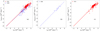 |
Fig. B.1. a: left: luminosity of the PAH feature at 6.2 μm as a function of the total IR luminosity. b: centre: [NeVI]7.65 μm line luminosity as a function of the total IR luminosity. c: right: luminosity of the PAH feature at 7.7 μm as a function of the total IR luminosity. The same legend as in Fig. 1 was used. |
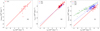 |
Fig. B.2. a: left: luminosity of the PAH feature at 8.6 μm as a function of the total IR luminosity. b: centre: luminosity of the H2 molecular line at 9.7 μm as a function of the total IR luminosity. c: right: [SIV]10.5 μm line luminosity as a function of the total IR luminosity. The same legend as in Fig. 1 was used. |
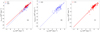 |
Fig. B.3. a: left: luminosity of the H2 molecular line at 12.28 μm as a function of the total IR luminosity. b: centre: [NeV]14.3 μm line luminosity as a function of the total IR luminosity. c: right: luminosity of the PAH feature at 17 μm as a function of the total IR luminosity. The same legend as in Fig. 1 was used. |
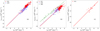 |
Fig. B.4. a: left: luminosity of the H2 molecular line at 17.03 μm as a function of the total IR luminosity. b: centre: [SIII]18.7 μm line luminosity as a function of the total IR luminosity. c: right: [FeIII]22.93 μm line luminosity as a function of the total IR luminosity. The same legend as in Fig. 1 was used. |
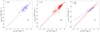 |
Fig. B.5. a: left: [NeV]24.3 μm line luminosity as a function of the total IR luminosity. b: centre: [FeII]25.99 μm line luminosity as a function of the total IR luminosity. c: right: luminosity of the H2 molecular line at 28.22 μm as a function of the total IR luminosity. The same legend as in Fig. 1 was used. |
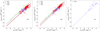 |
Fig. B.6. a: left: [SIII]33.4 μm line luminosity as a function of the total IR luminosity. b: centre: [SiII]34.8 μm line luminosity as a function of the total IR luminosity. c: right: [OIII]52 μm line luminosity as a function of the total IR luminosity. The same legend as in Fig. 1 was used. |
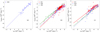 |
Fig. B.7. a: left: [NIII]57 μm line luminosity as a function of the total IR luminosity. b: centre: [OI]63.18 μm line luminosity as a function of the total IR luminosity. c: right: [NII]122 μm line luminosity as a function of the total IR luminosity. The same legend as in Fig. 1 was used. |
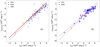 |
Fig. B.8. a: left: [OI]145 μm line luminosity as a function of the total IR luminosity. b: right: [NII]205 μm line luminosity as a function of the total IR luminosity. The same legend as in Fig. 1 was used. |
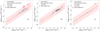 |
Fig. B.9. a: left: comparison between the local LIR–L[NII]122 relation for local SFGs (black dashed line) and high-redshift detections of [NII]122 μm line. The shaded area shows the 95% prediction interval for the local relation. The pink + sign indicates a detection for the [NII]122 μm line (De Breuck et al. 2019), while symbols with arrows indicate upper limits for high-redshift sources (Harikane et al. 2020). b: centre: comparison between the local LIR–L[OI]63 relation for local SFGs (black dashed line) and high-redshift detections of the [OI]63 μm line (pink symbol Rybak et al. 2020). c: right: comparison between the local LIR–L[OI]145 relation for local SFGs (black dashed line) and high-redshift detections of [OI]145 μm line (pink symbol De Breuck et al. 2019). The shaded area shows the 95% prediction interval for the local relation. Grey stars show local SFGs, while grey triangles show local LMGs. |
Appendix C: [NeV]14.3 μm as BHAR tracer and discussion on the use of the mid-ionisation lines
In this section, following what is done in Sect. 3.3, we report the results for the [NeV]14.3 μm line as BHAR tracer. In particular, starting from the total sample of Tommasin et al. (2008, 2010), excluding Compton-thick objects, we obtain a sample of 38 objects. The correlation between the [NeV]14.3 μm line luminosity and the 2−10 keV X-ray luminosity is shown in Fig. C.1a and is expressed by the following equation:
![Mathematical equation: $$ \begin{aligned} \log \left(\frac{L_{\rm X}}{10^{41}\,\mathrm{erg\,s}^{-1}}\right)=&(2.58 \pm 0.10)\nonumber \\&+(1.11 \pm 0.13)\log \left(\frac{L_{\rm [NeV]14.3}}{10^{41}\,\mathrm{erg\,s}^{-1}}\right), \end{aligned} $$](/articles/aa/full_html/2021/09/aa40696-21/aa40696-21-eq26.gif) (C.1)
(C.1)
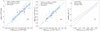 |
Fig. C.1. a: left: linear correlation between the [NeV]14.3 μm and the 2−10 keV X-ray luminosity. Blue squares show the AGN sample, and the shaded area shows the 95% confidence interval for the relation. b: centre: linear correlation between the [NeV]14.3 μm line luminosity and the 19 μm luminosity. c: right: comparison between the [NeV]14.3 μm line luminosity and the BHAR derived from the bolometric corrections by Spinoglio et al. (1995, green solid line), Marconi et al. (2004, red dotted line), and Lusso et al. (2012, blue dashed line). |
with a Pearson r coefficient of r = 0.79. From this result, we then apply the bolometric corrections by Marconi et al. (2004) and Lusso et al. (2012) to the 2−10 keV X-ray luminosity, in order to obtain the bolometric luminosity of the AGN. From the bolometric luminosities we then calculate the linear correlation linking the [NeV]14.3 μm line luminosity to the BHAR, with LAGN = ηṀBHc2. Assuming a radiative efficiency of η = 0.1, in Eq. (C.2) we report the linear correlation applying the bolometric correction from Lusso et al. (2012), and in Eq. (C.3) the one applying the Marconi et al. (2004) bolometric correction, and the relative Pearson r coefficient:
![Mathematical equation: $$ \begin{aligned} \log \left(\frac{\dot{M}_{\rm BH}}{{M}_{\odot }\,\mathrm{yr}^{-1}}\right)=&(-1.0 \pm 0.10)\nonumber \\&+(1.04 \pm 0.13)\log \left(\frac{L_{\rm [NeV]14.3}}{10^{41}\,\mathrm{erg\,s}^{-1}}\right),\,\,r=0.76, \end{aligned} $$](/articles/aa/full_html/2021/09/aa40696-21/aa40696-21-eq27.gif) (C.2)
(C.2)
![Mathematical equation: $$ \begin{aligned} \log \left(\frac{\dot{M}_{\rm BH}}{{M}_{\odot }\,\mathrm{yr}^{-1}}\right)=&(-0.73 \pm 0.17)\nonumber \\&+(1.49 \pm 0.13)\log \left(\frac{L_{\rm [NeV]14.3}}{10^{41}\,\mathrm{erg\,s}^{-1}}\right),\,\,r=0.78. \end{aligned} $$](/articles/aa/full_html/2021/09/aa40696-21/aa40696-21-eq28.gif) (C.3)
(C.3)
We then analysed the correlation between the [NeV]14.3 μm line with the luminosity at 19 μm following the work by Tommasin et al. (2010). As in Sect. 3.3, we only selected the sources with an AGN component at 19 μm equal to or above 85%, obtaining a sub-sample of 32 objects. The correlation between the [NeV]14.3 μm line luminosity and the 19 μm luminosity is shown in Fig. C.1b and expressed by
![Mathematical equation: $$ \begin{aligned} \log \left(\frac{L_{19}}{10^{41}\,\mathrm{erg\,s}^{-1}}\right)=&(3.09 \pm 0.06)\nonumber \\&+(1.01 \pm 0.10)\log \left(\frac{L_{\rm [NeV]14.3}}{10^{41}\,\mathrm{erg\,s}^{-1}}\right), \end{aligned} $$](/articles/aa/full_html/2021/09/aa40696-21/aa40696-21-eq29.gif) (C.4)
(C.4)
with a Pearson r coefficient of r = 0.85. We then calculate the bolometric luminosity from the monochromatic 12 μm luminosity extracted from Deo et al. (2009) using the relation by Spinoglio et al. (1995). From the bolometric luminosity we determine the BHAR and its relation to the [NeV]14.3 μm line luminosity, obtaining:
![Mathematical equation: $$ \begin{aligned} \log \left(\frac{\dot{M}_{\rm BH}}{{M}_{\odot }\,\mathrm{yr}^{-1}}\right)=&(-0.66 \pm 0.11)\nonumber \\&+(1.05 \pm 0.19)\log \left(\frac{L_{\rm [NeV]14.3}}{10^{41}\,\mathrm{erg\,s}^{-1}}\right),\,\,r=0.68 \end{aligned} $$](/articles/aa/full_html/2021/09/aa40696-21/aa40696-21-eq30.gif) (C.5)
(C.5)
for a sample of 26 objects, where r is the Pearson coefficient. The small number of objects used to derive this relation is due to the lack of data for the determination of the continuum at 12 μm.
In Fig. C.1c, we compare the three different relations derived to determine the BHAR from the [NeV]14.3 μm line luminosity. As in Sect. 3.3, we also find good agreement between the results obtained with the Lusso et al. (2012) and Spinoglio et al. (1995) bolometric corrections for this line, while the Marconi et al. (2004) bolometric correction produces a significantly steeper relationship.
As presented in Sect. 3.3 and here, high-ionisation lines, with an ionisation potential above the threshold of doubly ionised helium (54.4 eV) can only be efficiently produced by AGN activity, and thus are optimal BHAR tracers. Mid-ionisation lines, however, are partially affected by AGN activity, and could in theory be used as tracers for the BHAR. For this reason, we tested two mid-ionisation lines, namely the [SIV]10.5 μm line and the [NeIII]15.6 μm line, to evaluate their use as tracers for the X-ray luminosity in the 2−10 keV interval. Starting from the sample of Tommasin et al. (2008, 2010), as in Sect. 3.3, we excluded all Compton-thick objects and obtained a sub-sample of 44 objects for the [NeIII] line and of 39 objects for the [SIV] line. Figure C.2a shows the correlation between the [NeIII] line luminosity and the 2−10 keV X-ray luminosity, expressed as follows:
![Mathematical equation: $$ \begin{aligned} \log \left(\frac{L_{\rm X}}{10^{41}\,\mathrm{erg\,s}^{-1}}\right)=&(2.20 \pm 0.10)\nonumber \\&+(1.33 \pm 0.13)\log \left(\frac{L_{\rm [NeIII]15.6}}{10^{41}\,\mathrm{erg\,s}^{-1}}\right)\cdot \end{aligned} $$](/articles/aa/full_html/2021/09/aa40696-21/aa40696-21-eq31.gif) (C.6)
(C.6)
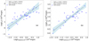 |
Fig. C.2. a: left: linear correlation between the [NeIII]15.6 μm and the 2−10 keV X-ray luminosity. Blue squares show the AGN sample, and the shaded area shows the 95% confidence interval for the relation. b: right: linear correlation between the [SIV]10.5 μm and the 2−10 keV X-ray luminosity. |
The correlation of the [SIV]10.5 μm line with the 2−10 keV X-ray luminosity, shown in Fig. C.2b, can be expressed as follows:
![Mathematical equation: $$ \begin{aligned} \log \left(\frac{L_{\rm X}}{10^{41}\,\mathrm{erg\,s}^{-1}}\right)=&(2.51 \pm 0.09)\nonumber \\&+(0.98 \pm 0.10)\log \left(\frac{L_{\rm [SIV]10.5}}{10^{41}\,\mathrm{erg\,s}^{-1}}\right)\cdot \end{aligned} $$](/articles/aa/full_html/2021/09/aa40696-21/aa40696-21-eq32.gif) (C.7)
(C.7)
For both correlations, we find a low Pearson correlation coefficient, equal to r = 0.63, lower than the values found for [OIV] (r = 0.87) and the [NeV] lines (r = 0.79 and r = 0.84, for the 14.3 μm and 24.3 μm lines, respectively). This suggests that, while mid-ionisation lines can correlate with the X-ray luminosity, they may suffer from contributions due to star formation activity, and thus are far less reliable as BHAR proxies. In particular, AGN sources in low-metallicity SFGs would have a significant contamination of the [SIV] and [NeIII] lines from the stellar population, as shown by the LMG in our sample (Figs. 1c and B.2c), in contrast with the [OIV] and [NeV] lines.
Appendix D: Line and PAH calibrations
New calibration obtained for fine-structure lines and PAH bands.
Appendix E: Differences with previous results
Here, we analyse the differences of the line calibrations obtained in this work with respect to those of Spinoglio et al. (2012, 2014) and Gruppioni et al. (2016).
When considering the results by Spinoglio et al. (2012), we only analyse the fine-structure lines in the 50−160 μm spectral interval, for which these authors consider an heterogeneous sample of both AGN and SFG, while in this work we consider three classes of galaxies. When comparing the results, we consider the calibrations obtained by Spinoglio et al. (2012) and compare them to our results for AGN and SFG. For this comparison, we apply the ordinary least-squares method to our samples, which was used in Spinoglio et al. (2012) to derive their correlations. Figure E.1 shows the comparison for the [OIII]52 μm, [NIII]57 μm, and [OI]63 μm lines; Fig. E.2 shows the comparison for the [OIII]88 μm, [NII]122 μm, and [OI]145 μm lines; and Fig. E.3 shows the comparison for the [CII]158 μm line.
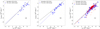 |
Fig. E.1. a: left: [OIII]52 μm line luminosity versus the total IR luminosity. b: centre: [NIII]57 μm line luminosity versus the total IR luminosity. c: right: [OI]63 μm line luminosity versus the total IR luminosity. In the figures, blue squares represent AGN while red stars show the SFG sample. The dashed blue line represents the linear correlation for the AGN sample, the dot-dashed red line shows the relation for SFG, and the black solid line the relation shows the relation obtained by Spinoglio et al. (2012, 2014). |
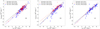 |
Fig. E.2. a: left: [OIII]88 μm line luminosity versus the total IR luminosity. b: centre: [NII]122 μm line luminosity versus the total IR luminosity. c: right: [OI]145 μm line luminosity versus the total IR luminosity. The same legend as in Fig. E.1 was used. |
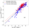 |
Fig. E.3. a: [CII]158 μm line luminosity versus the total IR luminosity. The same legend as in Fig. E.1 was used. |
When compared to our AGN sample, the results are consistent within the errors, except for the [NII]57 μm and [OIII]88 μm lines, where the slopes are comparable within 2σ of each other. If compared to the SFG results, we obtain results comparable within the errors except for [OIII]88 μm and [NII]122 μm lines, for which the slopes are comparable within 2σ of each other.
When considering the results presented by Gruppioni et al. (2016), we took advantage of the published catalogue and applied the orthogonal distance regression to the sample presented by the authors. Gruppioni et al. (2016) presented a sample of 76 AGN, which were divided in two sub-samples depending on the fraction of 5−40 μm luminosity produced by the active nucleus [fAGN(5 − 40 μm)]. In particular, there are 30 objects with fAGN(5 − 40 μm)≤0.4 and 43 objects with fAGN(5 − 40 μm) > 0.4.
Figures E.4–E.7 show the comparison for the relations calculated for the fAGN(5−40 μm) > 0.4 sub-sample, and Figs. E.8–E.11 show the comparison for the relations calculated for the fAGN(5−40 μm) ≤ 0.4 sub-sample.
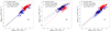 |
Fig. E.4. a: left: PAH 6.2 μm luminosity versus the total IR luminosity. Blue squares represent AGN, red stars SFGs, and black circles show the sample of Gruppioni et al. (2016). The dashed blue line represents the linear relation for AGN, the dot-dashed red line the relation for SFG, and the black solid line the relation for the Gruppioni et al. (2016) sample. b: centre: [SIV]10.5 μm luminosity versus the total IR luminosity. c: right: PAH 11.3 μm luminosity versus the total IR luminosity. In all three figures, the Gruppioni et al. (2016) sample was limited to AGN fractions > 0.4 in the 5−40 μm spectral interval (see Sect. 4.3). |
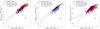 |
Fig. E.5. a: left: [NeII]12.8 μm line luminosity versus the total IR luminosity. b: centre: [NeV]14.3 μm line versus the total IR luminosity. c: right: [NeIII]15.6 μm line luminosity versus the total IR luminosity. In all three figures, the Gruppioni et al. (2016) sample was limited to AGN fractions > 0.4 in the 5−40 μm spectral interval (see Sect. 4.3). The same legend as in Fig. E.4 was used. |
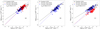 |
Fig. E.6. a: left: [SIII]18.7 μm line luminosity versus the total IR luminosity. b: centre: [NeV]24.3 μm line luminosity versus the total IR luminosity. c: right: [OIV]25.9 μm line luminosity versus the total IR luminosity. In all three figures, the Gruppioni et al. (2016) sample was limited to AGN fractions > 0.4 in the 5−40 μm spectral interval (see Sect. 4.3). The same legend as in Fig. E.4 was used. |
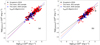 |
Fig. E.7. a: left: [SIII]33.5 μm line luminosity versus the total IR luminosity. b: right: [SiII]34.8 μm line luminosity versus the total IR luminosity. In both figures, the Gruppioni et al. (2016) sample was limited to AGN fractions > 0.4 in the 5−40 μm spectral interval (see Sect. 4.3). The same legend as in Fig. E.4 was used. |
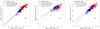 |
Fig. E.8. a: left: luminosity of the PAH feature at 6.2 μm versus the total IR luminosity. b: centre: [SIV]10.5 μm line luminosity as a function of the total IR luminosity. c: right: PAH 11.3 μm luminosity versus the total IR luminosity. In all figures, the Gruppioni et al. (2016) sample was limited to AGN fractions < 0.4 in the 5−40 μm spectral interval (see Sect. 4.3). The same legend as in Fig. E.4 was used. |
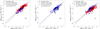 |
Fig. E.9. a: left: [NeII]12.8 μm line luminosity versus the total IR luminosity. b: centre: [NeV]14.3 μm line luminosity versus the total IR luminosity. c: right: [NeIII]15.6 μm line luminosity versus the total IR luminosity. In all three figures, the Gruppioni et al. (2016) sample was limited to AGN fractions < 0.4 in the 5−40 μm spectral interval (see Sect. 4.3). The same legend as in Fig. E.4 was used. |
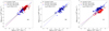 |
Fig. E.10. a: left: [SIII]18.7 μm line luminosity versus the total IR luminosity. b: centre: [NeV]24.3 μm line luminosity versus the total IR luminosity. c: right: [OIV]25.9 μm line luminosity versus the total IR luminosity. In all three figures, the Gruppioni et al. (2016) sample was limited to AGN fractions < 0.4 in the 5−40 μm spectral interval (see Sect. 4.3). The same legend as in Fig. E.4 was used. |
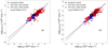 |
Fig. E.11. a: left: [SIII]33.5 μm line luminosity versus the total IR luminosity. b: right: [SiII]34.8 μm line luminosity versus the total IR luminosity. In both figures, the Gruppioni et al. (2016) sample was limited to AGN fractions < 0.4 in the 5−40 μm spectral interval (see Sect. 4.3). The same legend as in Fig. E.4 was used. |
As a general trend, our sample of AGN and the sample by Gruppioni et al. (2016) occupy the same region in the LIR–Lline space. We note that while the data to calculate the correlations were available in the literature, Gruppioni et al. (2016) only presented the correlations for [NeV]14.3, 24.3 μm, [NeIII]15.6 μm, and [OIV]25.9 μm for the fAGN(5−40 μm) > 0.4 sub-sample. For these relations, we find that our results show steeper slopes, but these are consistent within 3σ of each other.
For the fAGN(5−40 μm) ≤ 0.4 sub-sample, there is a better agreement between the relations, which are comparable within the errors. A significant difference in slope is present for the [NeV]24.3 μm line, for which the relations are comparable within 3σ, and for the [SIV]10.5 μm line, comparable within 2σ.
If we compare the results obtained using the Gruppioni et al. (2016) sample with the results we obtained using the SFG sample, we find comparable results for the PAH features for the fAGN(5−40 μm) > 0.4 and for all lines in the fAGN(5−40 μm) ≤ 0.4 sub-sample, excluding the [SIV]10.5 μm and [OIV]25.9 μm lines.
All Tables
Characteristics of the samples associated with the different spectral classes used in this analysis.
All Figures
|
Fig. 1. a: [CII]158 μm line luminosity as a function of the total IR luminosity. Blue squares represent detections in AGN, red stars indicate SFGs, and green triangles LMGs. The solid red line represents the linear relation calculated for SFGs, the blue dotted line shows the relation for AGN, and the green dashed line the one for LMGs. b: [NeII]12.8 μm line luminosity as a function of the total IR luminosity. c: [NeIII]15.6 μm line luminosity as a function of the total IR luminosity. In b and c, we use the same notations as in a. |
| In the text | |
|
Fig. 2. a: [OIII]88 μm line luminosity as a function of the total IR luminosity. b: [OIV]25.9 μm line luminosity as a function of the total IR luminosity. c: luminosity of the PAH feature at 11.3 μm as a function of the total IR luminosity. The same legend as in Fig. 1 was used. |
| In the text | |
|
Fig. 3. a: correlation between the [CII]158 μm line luminosity and the SFR derived from the total LIR. Red stars represent SFG, and green triangles represent the LMG. Purple squares show the ULIRG population of SFG, and the shaded green area indicates the 95% confidence interval. b: comparison of the log L[CII]–log(SFR) relation obtained in this work (black solid line) with the results obtained by De Looze et al. (2014); the green dashed line represents a sample of HII or SFGs, the blue diamond line shows the results for the low-metallicity dwarf sample, and the pink dash-dotted line considers the whole sample. The red dotted line shows the results obtained by Sargsyan et al. (2012). c: correlation between the [NeII]12.8 μm and [NeIII]15.6 μm summed emission lines’ luminosity, in units of 1041 erg s−1, and the SFR derived from the total IR luminosity (black dashed line) for SFGs (red star) and from the Hα luminosity (corrected for the IR luminosity) for LMGs (green triangles). The shaded green area indicates the 95% confidence interval. The purple squares highlight the ULIRG population in the SFG sample. The blue dashed line shows the results obtained by Zhuang et al. (2019) for the same relation. |
| In the text | |
|
Fig. 4. Correlation between the [OI]63 μm and [OIII]88 μm summed emission line luminosities, in units of 1041 erg s−1, and the SFR derived from the total IR luminosity (black dashed line) for a composite sample of SFGs (red stars) and from the Hα luminosity (corrected for the IR luminosity) for LMG (green triangles). Purple squares indicate the sample of ULIRGs included in the SFG sample. |
| In the text | |
|
Fig. 5. a: correlation between the [SIV]10.5 μm and [SIII]18.7 μm summed emission line luminosity, expressed in units of 1041 erg s−1, and the SFR derived from the total IR luminosity (black dashed line) for a composite catalogue of SFGs (red star) and from the Hα luminosity (corrected for the IR luminosity) for LMGs (green triangles). The shaded green areas in the three plots indicate the 95% confidence interval. b: correlation between the [NeII]12.8 μm and [SIV]10.5 μm summed luminosities and the SFR derived from the total IR luminosity (black dashed line) for SFGs (red star) and from the Hα luminosity (corrected for the IR luminosity) for LMGs (green triangles). c: correlation between the [NeIII]15.6 μm and [SIII]18.7 μm summed emission lines and the SFR derived from the total IR luminosity (black dashed line) for SFG (red star) and from the Hα luminosity (corrected for the IR luminosity) for LMG (green triangles). In all three figures, the purple squares highlight the ULIRG population in the SFG sample. |
| In the text | |
|
Fig. 6. a: correlation between the PAH emission feature at 6.2 μm, expressed in units of 1041 erg s−1 and the SFR derived from the total IR luminosity (black line) for a composite catalogue of SFGs (red star) and AGN-dominated galaxies (blue square). The shaded area in the three plots indicates the 95% confidence interval. b: correlation between the PAH emission feature at 11.3 μm, expressed in units of 1041 erg s−1 and the SFR derived from the total IR luminosity (black line) for a composite catalogue of SFGs (red star) and AGN-dominated galaxies (blue square). Panels a and b: we exclude ULIRGs from both AGN and SFG samples due to the known PAH deficit in these sources, as well as AGN with luminosities above 1045 erg s−1, which could dominate the IR continuum used to estimate the SFR. c: comparison of the relation between PAH total luminosity and SFR derived by Shipley et al. (2016) (black solid line) and using our sample (red dashed line). Red stars indicate SFG, purple squares indicate the ULIRG sub-sample included in the GOALS sample, and grey circles represent a sample of local galaxies used in Xie & Ho (2019). |
| In the text | |
|
Fig. 7. a: correlation between the H2 molecular line at 9.67 μm, expressed in units of 1041 erg s−1, and the SFR derived from the total IR luminosity (black line) for a catalogue of SFGs (red star). b: correlation between the H2 molecular line at 12.28 μm, expressed in units of 1041 erg s−1, and the SFR derived from the total IR luminosity (black line) for a catalogue of SFGs (red star). The green triangle shows LMG detection, which was not used to derive the correlation. c: correlation between the H2 molecular line at 17.03 μm, expressed in units of 1041 erg s−1, and the SFR derived from the total IR luminosity (black line) for a catalogue of SFGs (red star). In all three figures, the shaded areas show the 95% confidence interval of the relations, and the purple squares highlight the ULIRG population in the SFG sample. |
| In the text | |
|
Fig. 8. a: linear correlation between the [OIV]25.9 μm and the 2−10 keV X-ray luminosity. b: linear correlation between the [NeV]24.3 μm line luminosity and the 2−10 keV X-ray luminosity. c: linear correlation between the [OIV]25.9 μm line luminosity and the 19 μm luminosity. All luminosities are expressed in units of 1041 erg s−1. |
| In the text | |
|
Fig. 9. a: linear correlation between the [NeV]24.3 μm line luminosity and the 19 μm luminosity, expressed in units of 1041 erg s−1. b: comparison of the three different relations between the [OIV]25.9 μm line luminosity and the BHAR: the blue dashed line reports the relation obtained from the Lusso et al. (2012) bolometric correction, the red dotted line the relation from the Marconi et al. (2004) bolometric correction, and the green solid line the results from the Spinoglio et al. (1995) correction. c: same as panel a, but for the [NeV]24.3 μm line. |
| In the text | |
|
Fig. 10. Comparison of the ratio between the SFR obtained using the [NeII]+[NeIII] tracer and the SFR obtained using the PAH feature at 11.3 μm against the EW of the PAH feature at 6.2 μm for the GOALS sample. The colour gradient indicates the percentage of the AGN component in each object as determined by mid-IR tracers (Díaz-Santos et al. 2017). The black dashed line shows the mean value of the SFR ratio for the population, with the shaded area indicating where the 50% of the entire sample is located. The red dotted lines represent the 1σ interval around the mean value. |
| In the text | |
|
Fig. 11. a: comparison between the LIR–L[CII]158 relation (black dashed line) for local AGN dominated galaxies (grey squares) and high-redshift detections for QSOs (blue symbols). The shaded area shows the 95% prediction interval. b: same for high-redshift starburst galaxies (pink symbols). c: comparison of the local log(L[CII]–log(SFR) relation (black dashed line) and L[CII]–SFR values of high-redshift sources (pink symbols). Grey dots represent local SFGs. The shaded area shows the 95% prediction interval for the local relation. |
| In the text | |
|
Fig. 12. a: comparison between the LIR–L[OIII]88 relation (black dashed line) for local AGN-dominated galaxies (grey squares) and high-redshift detections for QSOs (blue symbols). b: comparison between the LIR–L[OIII]88 relation (red dashed line) for local SFG (grey stars) and high-redshift detections for starburst galaxies (pink symbols). The red shaded area shows the 95% prediction interval of this relation. For comparison, the green dashed line shows the LIR–L[OIII]88 relation for local LMG, with grey squares indicating local LMGs and the green shaded area giving the 95% prediction interval for this relation. c: comparison of the local LIR–L[NII]205 relation (black dashed line) for high-redshift detections of SFGs (pink symbols). Grey stars represent local SFGs. The shaded area in each figure shows the 95% prediction interval for the local relation. |
| In the text | |
|
Fig. 13. Left: observability of key mid-IR (dashed lines) lines compared to the JWST-MIRI instrument (shaded area) in the 0−1.6 redshift interval. Right: observability of key far-IR (dashed lines) lines compared to the ALMA bands (shaded area) in the 1−8 redshift interval. Dots represent current detection for each line. |
| In the text | |
|
Fig. B.1. a: left: luminosity of the PAH feature at 6.2 μm as a function of the total IR luminosity. b: centre: [NeVI]7.65 μm line luminosity as a function of the total IR luminosity. c: right: luminosity of the PAH feature at 7.7 μm as a function of the total IR luminosity. The same legend as in Fig. 1 was used. |
| In the text | |
|
Fig. B.2. a: left: luminosity of the PAH feature at 8.6 μm as a function of the total IR luminosity. b: centre: luminosity of the H2 molecular line at 9.7 μm as a function of the total IR luminosity. c: right: [SIV]10.5 μm line luminosity as a function of the total IR luminosity. The same legend as in Fig. 1 was used. |
| In the text | |
|
Fig. B.3. a: left: luminosity of the H2 molecular line at 12.28 μm as a function of the total IR luminosity. b: centre: [NeV]14.3 μm line luminosity as a function of the total IR luminosity. c: right: luminosity of the PAH feature at 17 μm as a function of the total IR luminosity. The same legend as in Fig. 1 was used. |
| In the text | |
|
Fig. B.4. a: left: luminosity of the H2 molecular line at 17.03 μm as a function of the total IR luminosity. b: centre: [SIII]18.7 μm line luminosity as a function of the total IR luminosity. c: right: [FeIII]22.93 μm line luminosity as a function of the total IR luminosity. The same legend as in Fig. 1 was used. |
| In the text | |
|
Fig. B.5. a: left: [NeV]24.3 μm line luminosity as a function of the total IR luminosity. b: centre: [FeII]25.99 μm line luminosity as a function of the total IR luminosity. c: right: luminosity of the H2 molecular line at 28.22 μm as a function of the total IR luminosity. The same legend as in Fig. 1 was used. |
| In the text | |
|
Fig. B.6. a: left: [SIII]33.4 μm line luminosity as a function of the total IR luminosity. b: centre: [SiII]34.8 μm line luminosity as a function of the total IR luminosity. c: right: [OIII]52 μm line luminosity as a function of the total IR luminosity. The same legend as in Fig. 1 was used. |
| In the text | |
|
Fig. B.7. a: left: [NIII]57 μm line luminosity as a function of the total IR luminosity. b: centre: [OI]63.18 μm line luminosity as a function of the total IR luminosity. c: right: [NII]122 μm line luminosity as a function of the total IR luminosity. The same legend as in Fig. 1 was used. |
| In the text | |
|
Fig. B.8. a: left: [OI]145 μm line luminosity as a function of the total IR luminosity. b: right: [NII]205 μm line luminosity as a function of the total IR luminosity. The same legend as in Fig. 1 was used. |
| In the text | |
|
Fig. B.9. a: left: comparison between the local LIR–L[NII]122 relation for local SFGs (black dashed line) and high-redshift detections of [NII]122 μm line. The shaded area shows the 95% prediction interval for the local relation. The pink + sign indicates a detection for the [NII]122 μm line (De Breuck et al. 2019), while symbols with arrows indicate upper limits for high-redshift sources (Harikane et al. 2020). b: centre: comparison between the local LIR–L[OI]63 relation for local SFGs (black dashed line) and high-redshift detections of the [OI]63 μm line (pink symbol Rybak et al. 2020). c: right: comparison between the local LIR–L[OI]145 relation for local SFGs (black dashed line) and high-redshift detections of [OI]145 μm line (pink symbol De Breuck et al. 2019). The shaded area shows the 95% prediction interval for the local relation. Grey stars show local SFGs, while grey triangles show local LMGs. |
| In the text | |
|
Fig. C.1. a: left: linear correlation between the [NeV]14.3 μm and the 2−10 keV X-ray luminosity. Blue squares show the AGN sample, and the shaded area shows the 95% confidence interval for the relation. b: centre: linear correlation between the [NeV]14.3 μm line luminosity and the 19 μm luminosity. c: right: comparison between the [NeV]14.3 μm line luminosity and the BHAR derived from the bolometric corrections by Spinoglio et al. (1995, green solid line), Marconi et al. (2004, red dotted line), and Lusso et al. (2012, blue dashed line). |
| In the text | |
|
Fig. C.2. a: left: linear correlation between the [NeIII]15.6 μm and the 2−10 keV X-ray luminosity. Blue squares show the AGN sample, and the shaded area shows the 95% confidence interval for the relation. b: right: linear correlation between the [SIV]10.5 μm and the 2−10 keV X-ray luminosity. |
| In the text | |
|
Fig. E.1. a: left: [OIII]52 μm line luminosity versus the total IR luminosity. b: centre: [NIII]57 μm line luminosity versus the total IR luminosity. c: right: [OI]63 μm line luminosity versus the total IR luminosity. In the figures, blue squares represent AGN while red stars show the SFG sample. The dashed blue line represents the linear correlation for the AGN sample, the dot-dashed red line shows the relation for SFG, and the black solid line the relation shows the relation obtained by Spinoglio et al. (2012, 2014). |
| In the text | |
|
Fig. E.2. a: left: [OIII]88 μm line luminosity versus the total IR luminosity. b: centre: [NII]122 μm line luminosity versus the total IR luminosity. c: right: [OI]145 μm line luminosity versus the total IR luminosity. The same legend as in Fig. E.1 was used. |
| In the text | |
|
Fig. E.3. a: [CII]158 μm line luminosity versus the total IR luminosity. The same legend as in Fig. E.1 was used. |
| In the text | |
|
Fig. E.4. a: left: PAH 6.2 μm luminosity versus the total IR luminosity. Blue squares represent AGN, red stars SFGs, and black circles show the sample of Gruppioni et al. (2016). The dashed blue line represents the linear relation for AGN, the dot-dashed red line the relation for SFG, and the black solid line the relation for the Gruppioni et al. (2016) sample. b: centre: [SIV]10.5 μm luminosity versus the total IR luminosity. c: right: PAH 11.3 μm luminosity versus the total IR luminosity. In all three figures, the Gruppioni et al. (2016) sample was limited to AGN fractions > 0.4 in the 5−40 μm spectral interval (see Sect. 4.3). |
| In the text | |
|
Fig. E.5. a: left: [NeII]12.8 μm line luminosity versus the total IR luminosity. b: centre: [NeV]14.3 μm line versus the total IR luminosity. c: right: [NeIII]15.6 μm line luminosity versus the total IR luminosity. In all three figures, the Gruppioni et al. (2016) sample was limited to AGN fractions > 0.4 in the 5−40 μm spectral interval (see Sect. 4.3). The same legend as in Fig. E.4 was used. |
| In the text | |
|
Fig. E.6. a: left: [SIII]18.7 μm line luminosity versus the total IR luminosity. b: centre: [NeV]24.3 μm line luminosity versus the total IR luminosity. c: right: [OIV]25.9 μm line luminosity versus the total IR luminosity. In all three figures, the Gruppioni et al. (2016) sample was limited to AGN fractions > 0.4 in the 5−40 μm spectral interval (see Sect. 4.3). The same legend as in Fig. E.4 was used. |
| In the text | |
|
Fig. E.7. a: left: [SIII]33.5 μm line luminosity versus the total IR luminosity. b: right: [SiII]34.8 μm line luminosity versus the total IR luminosity. In both figures, the Gruppioni et al. (2016) sample was limited to AGN fractions > 0.4 in the 5−40 μm spectral interval (see Sect. 4.3). The same legend as in Fig. E.4 was used. |
| In the text | |
|
Fig. E.8. a: left: luminosity of the PAH feature at 6.2 μm versus the total IR luminosity. b: centre: [SIV]10.5 μm line luminosity as a function of the total IR luminosity. c: right: PAH 11.3 μm luminosity versus the total IR luminosity. In all figures, the Gruppioni et al. (2016) sample was limited to AGN fractions < 0.4 in the 5−40 μm spectral interval (see Sect. 4.3). The same legend as in Fig. E.4 was used. |
| In the text | |
|
Fig. E.9. a: left: [NeII]12.8 μm line luminosity versus the total IR luminosity. b: centre: [NeV]14.3 μm line luminosity versus the total IR luminosity. c: right: [NeIII]15.6 μm line luminosity versus the total IR luminosity. In all three figures, the Gruppioni et al. (2016) sample was limited to AGN fractions < 0.4 in the 5−40 μm spectral interval (see Sect. 4.3). The same legend as in Fig. E.4 was used. |
| In the text | |
|
Fig. E.10. a: left: [SIII]18.7 μm line luminosity versus the total IR luminosity. b: centre: [NeV]24.3 μm line luminosity versus the total IR luminosity. c: right: [OIV]25.9 μm line luminosity versus the total IR luminosity. In all three figures, the Gruppioni et al. (2016) sample was limited to AGN fractions < 0.4 in the 5−40 μm spectral interval (see Sect. 4.3). The same legend as in Fig. E.4 was used. |
| In the text | |
|
Fig. E.11. a: left: [SIII]33.5 μm line luminosity versus the total IR luminosity. b: right: [SiII]34.8 μm line luminosity versus the total IR luminosity. In both figures, the Gruppioni et al. (2016) sample was limited to AGN fractions < 0.4 in the 5−40 μm spectral interval (see Sect. 4.3). The same legend as in Fig. E.4 was used. |
| In the text | |
Current usage metrics show cumulative count of Article Views (full-text article views including HTML views, PDF and ePub downloads, according to the available data) and Abstracts Views on Vision4Press platform.
Data correspond to usage on the plateform after 2015. The current usage metrics is available 48-96 hours after online publication and is updated daily on week days.
Initial download of the metrics may take a while.