| Issue |
A&A
Volume 651, July 2021
|
|
|---|---|---|
| Article Number | A42 | |
| Number of page(s) | 28 | |
| Section | Extragalactic astronomy | |
| DOI | https://doi.org/10.1051/0004-6361/202140955 | |
| Published online | 12 July 2021 | |
Physics of ULIRGs with MUSE and ALMA: The PUMA project
II. Are local ULIRGs powered by AGN? The subkiloparsec view of the 220 GHz continuum
1
Centro de Astrobiología (CSIC-INTA), Ctra. de Ajalvir, Km 4, 28850 Torrejón de Ardoz, Madrid, Spain
e-mail: miguel.pereira@cab.inta-csic.es
2
Observatorio Astronómico Nacional (OAN-IGN)-Observatorio de Madrid, Alfonso XII, 3, 28014 Madrid, Spain
3
Universidad de Alcalá, Departamento de Física y Matemáticas, Campus Universitario, 28871 Alcalá de Henares, Madrid, Spain
4
INAF – Osservatorio Astrofisico di Arcetri, Largo Enrico Fermi 5, 50125 Firenze, Italy
5
Centro de Astrobiología (CSIC-INTA), ESAC Campus, 28692 Villanueva de la Cañada, Madrid, Spain
6
Department of Space, Earth and Environment, Onsala Space Observatory, Chalmers University of Technology, 439 92 Onsala, Sweden
7
LERMA, Obs. de Paris, PSL Univ., Collége de France, CNRS, Sorbonne Univ., Paris, France
8
Department of Physics, University of Oxford, Keble Road, Oxford OX1 3RH, UK
9
Leiden Observatory, Leiden University, PO Box 9513 2300 RA Leiden, The Netherlands
Received:
31
March
2021
Accepted:
9
May
2021
We analyze new high-resolution (400 pc) ∼220 GHz continuum and CO(2–1) Atacama Large Millimeter Array (ALMA) observations of a representative sample of 23 local (z < 0.165) ultra-luminous infrared systems (ULIRGs; 34 individual nuclei) as part of the “Physics of ULIRGs with MUSE and ALMA” (PUMA) project. The deconvolved half-light radii of the ∼220 GHz continuum sources, rcont, are between < 60 pc and 350 pc (median 80–100 pc). We associate these regions with the regions emitting the bulk of the infrared luminosity (LIR). The good agreement, within a factor of 2, between the observed ∼220 GHz fluxes and the extrapolation of the infrared gray-body as well as the small contributions from synchrotron and free–free emission support this assumption. The cold molecular gas emission sizes, rCO, are between 60 and 700 pc and are similar in advanced mergers and early interacting systems. On average, rCO are ∼2.5 times larger than rcont. Using these measurements, we derived the nuclear LIR and cold molecular gas surface densities (ΣLIR = 1011.5 − 1014.3 L⊙ kpc−2 and ΣH2 = 102.9 − 104.2 M⊙ pc−2, respectively). Assuming that the LIR is produced by star formation, the median ΣLIR corresponds to ΣSFR = 2500 M⊙ yr−1 kpc−2. This ΣSFR implies extremely short depletion times, ΣH2/ΣSFR < 1–15 Myr, and unphysical star formation efficiencies > 1 for 70% of the sample. Therefore, this favors the presence of an obscured active galactic nucleus (AGN) in these objects that could dominate the LIR. We also classify the ULIRG nuclei in two groups: (a) compact nuclei (rcont < 120 pc) with high mid-infrared excess emission (ΔL6−20 μm/LIR) found in optically classified AGN; and (b) nuclei following a relation with decreasing ΔL6−20 μm/LIR for decreasing rcont. The majority, 60%, of the nuclei in interacting systems lie in the low-rcont end (<120 pc) of this relation, while this is the case for only 30% of the mergers. This suggests that in the early stages of the interaction, the activity occurs in a very compact and dust-obscured region while, in more advanced merger stages, the activity is more extended, unless an optically detected AGN is present. Approximately two-thirds of the nuclei have nuclear radiation pressures above the Eddington limit. This is consistent with the ubiquitous detection of massive outflows in local ULIRGs and supports the importance of the radiation pressure in the outflow launching process.
Key words: galaxies: evolution / galaxies: interactions / galaxies: nuclei / infrared: galaxies
© ESO 2021
1. Introduction
Ultraluminous infrared galaxies (ULIRGs; LIR > 1012 L⊙) are among the most luminous objects in the local Universe. The majority of local ULIRGs are major gas-rich mergers at different evolutionary stages: from interacting systems with two nuclei separated by few kiloparsecs to more advanced mergers with a single nucleus (see Lonsdale et al. 2006 and references therein). A classic evolutionary scenario suggests that merging ULIRGs evolve into a quasar that quenches the star formation (SF) and, after that, the merger remnant becomes an intermediate-mass elliptical galaxy (e.g., Sanders et al. 1988; Springel et al. 2005). However, recent observations and simulations indicate that mergers do not always quench the SF and also that disks can regrow in mergers remnants (e.g., Ueda et al. 2014; Weigel et al. 2017; Weinberger et al. 2018). This suggests that ULIRGs can have more varied evolutionary paths than suggested by the classic scenario. Local ULIRGs might also be scaled down versions of the dusty star-forming mergers detected at z > 2 (e.g., Casey et al. 2014). Therefore, local ULIRGs are excellent targets for detailed studies of the physical processes that shape the, possibly diverse, evolutionary paths of merging gas-rich galaxies, which were important in the high-z universe.
One key property of local ULIRGs are their extremely compact (<1 kpc; e.g., Condon et al. 1991; Soifer et al. 2000) and dust obscured nuclei (Av > 1000 mag in some cases based on their nuclear molecular gas column densities; e.g., González-Alfonso et al. 2015). Because of this extreme obscuration most of the radiation produced in their nuclei, either by an active galactic nucleus (AGN) or by SF, is absorbed by dust and re-emitted in the infrared (IR) spectral range. For this reason, it is not straightforward to determine the dominant power source (AGN vs. SF) of local ULIRGs. Mid-IR studies, which are less affected by extinction than optical and near-IR works, suggest that ULIRGs are mostly powered by SF (e.g., Genzel et al. 1998), although the AGN contribution increases with increasing luminosities (e.g., Nardini et al. 2008; Veilleux et al. 2009). However, for Av > 1000 mag, the mid-IR extinction is still very high, A15 μm > 50 mag (e.g., Jiang et al. 2006), and a large part of the emission could be completely obscured even in the mid-IR which. This could prevent an accurate determination of the AGN and SF contributions to the LIR of local ULIRGs using mid-IR observations.
Alternatively, it is possible to investigate what powers local ULIRGs by measuring the size of the region that emits the bulk of the LIR as well as the molecular gas content (i.e., the fuel for SF) of this region. These quantities are needed to determine the nuclear IR luminosity and gas surface densities. Finding IR luminosity densities well above the limit of a maximal starburst (e.g., Thompson et al. 2005) can be used to infer the presence of an obscured AGN and to estimate its luminosity (see e.g., Downes & Eckart 2007; Imanishi et al. 2011; Sakamoto et al. 2017).
In this paper, we analyze high-resolution (∼400 pc) Atacama Large Millimeter Array (ALMA) CO(2–1) and ∼220 GHz continuum observations of sample of 23 local ULIRGs. We measure the size of the ∼220 GHz (∼1400 μm) continuum, which we link with the bulk of the LIR in these sources, and we estimate the nuclear cold molecular gas content from the CO(2–1) emission. We use these results to calculate their nuclear luminosity and molecular gas densities.
These ALMA observations of a representative sample of local ULIRGs are part of the “Physics of ULIRGs with the Multi-Unit Spectroscopic Explorer (MUSE) and ALMA” (PUMA) project. The main goals of this project are: (a) to establish the impact of massive outflows in the evolution of ULIRGs (negative and positive feedback); and (b) to determine what drives this feedback (AGN vs. SF) during the entire merging process (from early stages to advanced mergers). To do so, we combine subkiloparsec resolution adaptive optics (AO) assisted Very Large Telescope (VLT) MUSE optical integral field spectroscopy and CO(2–1) ALMA data to trace the multiphase structure of the massive outflows as well as to investigate basic properties of the ULIRGs like their main power source. The first MUSE results on the spatially resolved stellar kinematics and the ionized outflow phase were presented by Perna et al. (2021) while the detailed analysis of the Arp 220 MUSE data was presented in Perna et al. (2020). Likewise, Pereira-Santaella et al. (2018) presented the first ALMA results on the spatially resolved cold molecular outflows detected in three of these local ULIRGs.
The paper is organized as follows. We briefly describe the PUMA sample in Sect. 2. The ALMA observations and data reduction are presented in Sect. 3. In Sect. 4, we derive the spatial properties of the ∼220 GHz continuum and the CO(2–1) emission, and fit the IR and radio spectral energy distributions (SEDs) of the ULIRGs. Section 5 investigates the origin of the high luminosity and molecular gas surface densities in the ULIRG nuclei, the relation between the ∼220 GHz continuum size with the mid-IR excess emission, the 9.7 μm silicate absorption, and the broad-band Infrared Astronomical Satellite (IRAS) colors. We also estimate the radiation pressure in these nuclei. The main conclusions are summarized in Sect. 6.
Throughout this article we assume the following cosmology: H0 = 70 km s−1 Mpc−1, Ωm = 0.3, and ΩΛ = 0.7.
2. Sample of local ULIRGs
The PUMA sample is a volume-limited (z < 0.165; d < 800 Mpc) representative sample of 25 local ULIRGs (38 individual nuclei). These objects were selected to examine the most relevant parameters for the feedback processes: (1) the main power source (AGN vs. SF); (2) the interaction stage (from interacting pairs to advanced mergers); and (3) the IR luminosity. The parent sample is the 1 Jy ULIRG sample (Kim et al. 1998) extended to southern objects by Duc et al. (1997). Our sample is limited to objects with Dec between −65° and +25° which is appropriate for ALMA. We selected 12 interacting systems (nuclear separation > 1 kpc) and 13 mergers with nuclear separations < 1 kpc. Half of the objects in each interaction stage category were selected to be dominated by AGN based on mid-IR spectroscopy (Veilleux et al. 2009; Spoon et al. 2013). The selected objects uniformly cover the ULIRG luminosity range between 1012.0 and 1012.7 L⊙. See Table 1 and Perna et al. (2021) for more details.
Sample of local ULIRGs.
So far, we have obtained ALMA CO(2–1) and ∼220 GHz continuum observations for 92% of the systems in the sample (23 systems with 34 individual nuclei). The CO(2–1) emission is detected in 33 nuclei and the continuum in 29 (see Sect. 4). In addition to our VLT/MUSE-AO optical integral field spectroscopy (Perna et al. 2020, 2021), the majority of the targets have extensive ancillary multiwavelength data which include mid- and far-IR (e.g., Veilleux et al. 2009; Spoon et al. 2013; Pearson et al. 2016; Chu et al. 2017), radio (e.g., Condon et al. 1998; Helfand et al. 2015), and X-ray (e.g., Iwasawa et al. 2011; Teng et al. 2015) observations.
3. Observations and data reduction
3.1. ALMA observations
We obtained ALMA 12-m array CO(2–1) 230.538 GHz and continuum observations for 23 out of the 25 PUMA ULIRGs. ALMA observations for the remaining two ULIRGs have been scheduled but are not available at the time of writing. These observations were mainly conducted as part of our programs 2015.1.00263.S, 2016.1.00170.S, and 2018.1.00699.S (PI: M. Pereira-Santaella). For 13120−5453 and F15327+2340 (Arp 220), we used archive data from programs 2016.1.00777.S (PI: K. Sliwa) and 2015.1.00113.S (PI: N. Scoville), respectively. In addition, we complemented this dataset with higher angular resolution data for 17208−0014 from program 2018.1.00486.S (PI: M. Pereira-Santaella). Observations of three of the ULIRGs in our sample (F12112+0305, F14348−1447, and F22491−1808) have already been presented in Pereira-Santaella et al. (2018), but we include them here for completeness.
We aimed to have a similar spatial resolution of ∼400 pc in all the systems, so the synthesized beam full-width half-maximum (FWHM) varies between 0 12 and 1″ depending on the distance of each target. We used a single 12-m array configuration with baselines set to achieve the required angular resolution. The maximum recoverable scale is about ten times the beam FWHM (i.e., 4 kpc). Depending on the redshift, the CO(2–1) transition lies in the ALMA Band 5 or Band 6. Details on the observations are listed in Table 2.
Summary of the continuum ALMA observations.
We defined four 1.875 GHz bandwidth spectral windows with 2–8 MHz (3–10 km s−1) channels, depending on the targeted spectral feature. One spectral window was centered at the sky frequency of 12CO(2–1) 230.538 GHz. The remaining spectral windows were centered at the frequency of nearby transitions (e.g., CS(5–4), H30α, SiO(5-4)) when possible or at a “line-free” spectral range.
We used the ALMA reduction software CASA (v5.6.1; Mcmullin et al. 2007) to calibrate the data using the standard pipeline. The absolute flux accuracy of Band 5 and 6 data is ∼10% (ALMA Technical Handbook). For the CO(2–1) spectral window, we subtracted a constant continuum level estimated from the line emission free channels in the uv plane. The data were cleaned using the TCLEAN CASA task and the Brigss weighting with robustness parameters between −0.5 and 2.0 to match the required ∼400 pc spatial resolution. For two systems (13120−5453 and 17208−0014), the largest synthesized beam provides a spatial resolution better than 400 pc, so we used the IMSMOOTH task to convolve the cubes with a Gaussian and obtained the desired spatial resolution. For F15327+2340 (Arp 220), we only used the compact configuration data which provide a ∼370 pc spatial resolution comparable to that of the other ULIRGs in our sample. The channel width of the final cubes is ∼10 km s−1 and the pixel sizes are about a sixth of the beam FWHM (i.e., between 20 and 120 mas). In addition to the line data cubes, we produced continuum images using spectral windows where no emission or absorption lines were present. The continuum sensitivities range from 18 to 290 μJy beam−1 with more sensitive data for the more distant objects (see Table 2).
In this paper, we primarily focus on the analysis of the continuum and CO(2–1) maps. In a future paper (Lamperti et al., in prep.), we will present the detailed analysis of the line data.
3.2. Ancillary Spitzer data
To complete the spectral energy distribution (SED) of the ULIRGs (Sect. 4.4), we used mid-IR Spitzer data. In particular we used the 5.2–38 μm low-resolution (R ∼ 60−130) spectra from the Infrared Spectrograph (IRS; Houck et al. 2004) and the 70 and 160 μm images from the Multiband Imaging Photometer (MIPS; Rieke et al. 2004).
We downloaded the calibrated IRS spectra for all the systems in our sample from the Cornell Atlas of Spitzer/Infrared Spectrograph Sources (CASSIS; Lebouteiller et al. 2011) and measured the flux at 34 μm, which is approximately at the middle point between the 24 and 70 μm photometric points in log scale and avoids the noisier long-wavelength edge of the IRS spectrum.
We also downloaded the calibrated MIPS images for five systems from the Spitzer Heritage Archive1. The ULIRG systems appear as point-sources at the MIPS angular resolution (18″ and 40″ at 70 and 160 μm, respectively). For the 70 μm image, we used a 35″ radius aperture and a 39–65″ background annulus and then multiplied the flux by 1.24 to account for the aperture correction factor (see Table 4.14 of the MIPS Instrument Handbook). For the 160 μm images, we subtracted a global background emission level and used a 60″ radius aperture. We applied a 1.40 aperture correction factor which is appropriate for sources with temperatures between 30 and 150 K (see Table 4.15 of the MIPS Instrument Handbook). The measured Spitzer IRS and MIPS fluxes are listed in Appendix A.
4. Data analysis
4.1. ALMA continuum model. Size and flux
We modeled the ALMA 220–250 GHz continuum images to determine the flux, size, and position of the detected emitting regions. In general, these regions are compact (FWHMs similar to the beam size) and their morphological structure is barely resolved. Therefore, we used simple models consisting of a point-source, a Gaussian, point-source + Gaussian, or two Gaussians. These models were convolved with the beam and compared with the observations to determine a χ2 value. Then, we minimized the χ2 by varying the fluxes, sizes, and positions of the model components.
We tried these four models for each nucleus and selected the one with the lowest reduced χ2. The best-fit models reproduce quite well the observed emission. The median (mean) reduced χ2 is 1.1 (1.4), the maximum is 3.1, and no significant structures are seen in the residual images (see Fig. 1). This figure also shows the best-fit model whose parameters are listed in Table 3. The best-fit positions are presented in Table 1. Based on these parameters, we computed the half-light radius of the ∼220 GHz continuum, rcont, which is defined as the radius of the region that contains 50% of the observed flux.
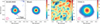 |
Fig. 1. ALMA continuum observation (first panel), best-fit model (second panel), residual emission after subtracting the continuum model (third panel), and the integrated CO(2–1) emission (moment 0) from Lamperti et al., in prep. (fourth panel) for 00188−0856 as an example. The two contour levels in the first panel indicate the 3σ and the 0.5×peak emission levels. In the second panel, the individual components of the best-fit model are presented as a black circle (point source model) and as a dashed ellipse (deconvolved Gaussian model). The black crosses in the first, third, and fourth panels mark the fit location of the continuum peak. The red hatched ellipses represent the beam FWHM. The units are μJy beam−1 for the continuum panels and Jy km s−1 beam−1 for the CO(2–1) panel. The continuum model fits for the whole sample are shown in Fig. B.1. |
ALMA continuum models.
For 11 nuclei whose model includes a point-source, the half-light radius is not well defined because the point source contributes > 50% to the total flux. Therefore, to estimate the size upper limit in these cases, we performed a series of simulations. First, we subtracted, when present, the extended Gaussian component of the model. Then, we used circular Gaussian models with fixed FWHM from 2 to 6 pixels2, that were convolved with the beam, and obtained the χ2 variation as function of the model FWHM. Finally, we estimated the 3σ FWHM upper limit as the FWHM at which the χ2 increases by 9.03 with respect to the minimum χ2. The FWHM upper limits are also included in Table 3.
Figure 2 shows the distribution of the half-light radius and the upper limits. The measured rcont range from < 50 pc to 350 pc with a median value of 80–100 pc. The rcont of AGN and non-AGN objects, based on optical spectroscopy, are similar.
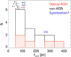 |
Fig. 2. Distribution of the ∼220 GHz continuum half-light radius (rcont; see Table 3). Upper limits are indicated with arrows. The red (black) histogram bars and arrows correspond to galaxies classified as AGN (non-AGN) from optical spectroscopy. The sizes of the systems whose ALMA flux might have high (>40%) nonthermal synchrotron contributions are marked in blue (see Sect. 5.1.2). |
Mid-IR observations already indicate that ULIRGs are very compact (<1 kpc; Soifer et al. 2000; Díaz-Santos et al. 2010; Alonso-Herrero et al. 2014, 2016; Imanishi et al. 2020). Our higher angular resolution ALMA continuum data suggest that they are even more compact.
4.2. Higher resolution observations
The CO(2–1) and 230 GHz continuum emission of F15327+2340 (Arp 220) have been observed by ALMA at much higher resolution (8 pc) than the data used in this paper. However, these data are still unpublished. Instead, we can compare with the 20–40 pc 2.7 mm (∼110 GHz) continuum observations presented by Scoville et al. (2017) and Sakamoto et al. (2017). These authors measure deconvolved Gaussian FWHM of 160–180 mas for the East nucleus and 74–114 mas for the West nucleus. From the low resolution data, we obtained 2 × rcont = 400 mas and < 260 mas for the East and West nuclei, respectively. Therefore, we recover a reliable upper limit size for the bright and compact source in the West nucleus. For the East nucleus, we derive a size two times larger. However, it is possible that part of extended emission detected in the low-resolution data is filtered out, or too faint, in the ten times higher resolution published observations.
In addition, 17208−0014 was observed as part of another program which aimed to obtain ∼100 pc spatial resolution CO(2–1) and continuum data. These observations will be analyzed in detail in a future paper. However, here we use the high resolution continuum data (120 pc vs. 400 pc), to test whether the source size derived from the low-resolution data (rcont < 75 pc for this object) is consistent with the size measured in the high-resolution data.
Figure 3 compares the low- and the high-resolution maps. The difference between the continuum fluxes in both images measured using a 1″ radius aperture is < 9% (42.7 ± 0.2 vs. 46.3 ± 0.3 mJy). This indicates that the higher resolution data do not miss significant low surface brightness emission. This figure also shows that the continuum emission peak measured in the original low-resolution data (Table 1) appears slightly shifted (30 mas or 26 pc) in the high-resolution image. This is possibly because now we start to spatially resolve the inner structure of the nucleus and multiple smaller regions appear.
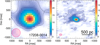 |
Fig. 3. Comparison between the 400 pc resolution 247 GHz continuum image analyzed in Sect. 4.1 (left panel) and the higher resolution (120 pc) data (right panel) available for 17208−0014. The black cross is the position of the center measured on the 400 pc image. The contours are as in Fig. 1. The hatched red ellipses correspond to the beam FWHM of each image. The color scales are in mJy beam−1. |
We applied the same model fitting procedure described in Sect. 4.1 to the higher resolution image. The original model consisted of a point source plus a Gaussian (see Table 3 and Fig. B.1). For the high-resolution data, we used two Gaussians since the emission core is resolved. This “core” Gaussian has a flux of 17.6 ± 1.1 mJy and a circularized FWHM of 74 ± 3 mas (62 pc; rcont = 31 pc). It contains about 40% of the 247 GHz continuum emission from 17208−0014, so the rcont < 75 pc upper limit we estimated from the low-resolution data (Table 3) seems to be consistent with what is observed at higher angular resolution. The result for these two objects supports that our method to estimate the rcont can produce realistic values, even below the beam size.
4.3. Nuclear molecular gas
Figures 1 and B.1 show that the CO(2–1) emission is more extended than the continuum and also that it has a more complex morphology. As a consequence, the simple set of models used to fit the continuum (Sect. 4.1) does not reproduce the CO(2–1) emission properly. Therefore, we considered a different approach to determine the size and flux of the nuclear CO(2–1) emission.
We used the CO(2–1) moment 0 maps (Lamperti et al., in prep.) to extract the flux in concentric apertures centered at the continuum peak. This produces an azimuthally averaged growth curve for the CO(2–1) emission (see Fig. 4). To fit this curve, we simulated a 2D circular Gaussian model, which was convolved with the beam, and we compared the model growth curve with the observed one. From this fit, we obtained the deconvolved circularized FWHM of the CO(2–1) emission and the nuclear flux. Then, we used a ULIRG-like αCO conversion factor (0.78 M⊙ (K km s−1 pc−2)−1) and a CO 2–1 to 1–0 ratio r21 = 0.91 (Bolatto et al. 2013) to estimate the molecular gas mass. We limited this growth curve to the central ∼1.5 kpc, so the most extended emission of the systems is not included in the measured flux. Nevertheless, we are mostly interested in the CO(2–1) sizes and fluxes of the nuclear regions detected in the continuum and these are well covered by the apertures used (∼700 pc aperture radius vs. rcont < 350 pc). The nuclear CO(2–1) deconvolved sizes, rCO, fluxes, molecular gas masses, and molecular gas surface densities, ΣH2, are presented in Table 4.
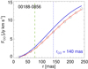 |
Fig. 4. Growth curve of the CO(2–1) moment 0 map for 00188−0856 as an example. The circles correspond to the observed flux within a circular aperture of radius r. The red line is the best fit model (Sect. 4.3). The deconvolved best fit profile is shown in blue and its effective radius, rCO = FWHM/2, is indicated by the vertical blue dotted line. The dashsed green line marks the ∼220 GHz continuum radius, rcont for comparison. The CO(2–1) model fits for the whole sample are shown in Fig. C.1. |
Nuclear CO(2–1) emission and cold molecular gas mass.
The CO(2–1) radius rCO ranges from 60 to 500 pc (median 320 pc). Figure 5 shows that rCO is larger then the continuum size rcont. The median rCO/rcont ratio is 2.5 ± 1.1. As for the continuum size, we do not find significant differences between the rCO of AGN and non-AGN nuclei. If we exclude the nuclei with upper limits for rcont, there is a good correlation between the CO and continuum sizes (Spearman’s rank correlation coefficient rs = 0.72, probability of no correlation p = 7 × 10⁻⁴). The best linear fit is rCO = (0.70 ± 15)×rcont + (240 ± 30) pc.
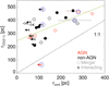 |
Fig. 5. Half light radius of the 220 GHz continuum rcont vs. 0.5 × FWHM of the CO(2–1) emission rCO. Red (black) symbols mark systems classified as AGN (non-AGN) based on optical spectroscopy. Filled symbols correspond to nuclei in interacting systems and empty symbols to nuclei in mergers (see Table 1). Blue encircled symbols are galaxies with excess nonthermal emission whose continuum size estimates might be inaccurate (Sect. 5.1.2). The green line is best linear fit excluding the nuclei with rcont upper limits. The dotted line indicates the 1:1 relation. |
4.4. Spectral energy distribution fit
4.4.1. IR SED
We fit the IR spectral energy distribution of these ULIRGs to determine the expected dust emission at the ALMA frequency (220–250 GHz ≡ 1400–1200 μm). We used published IR photometry from Herschel, Infrared Space Observatory (ISO), and IRAS (see Table 5), as well as Spitzer IRS and MIPS data (see Sect. 3.2 and Appendix A). For observations at similar wavelengths, we gave preference to the data with the highest angular resolution.
Far-IR and radio fluxes references
We fit the far-IR SED using a single-temperature gray-body (e.g., Eqs. (1) and (2) of Kovács et al. 2010). We assumed a fixed β = 1.8 (Planck Collaboration XXV 2011), but allowed the optical depth to vary. This model reproduces well the observed far-IR SED between 30 and 500 μm for most objects. At shorter wavelengths, some of these ULIRGs have excess mid-IR emission which has been associated with warmer dust due to an AGN (e.g., Nardini et al. 2009; Veilleux et al. 2009). Since we are interested in the longer wavelength emission to compare with the ALMA observation, we only used in the fit the photometric points between 34 and 500 μm to avoid any bias due to this mid-IR excess. We note that we excluded the ALMA continuum flux from the SED fit. For four systems (00509+1225, 01572+0009, F05189−2524, and F13451+1232), we started the fit at 70 μm because the excess mid-IR emission was clear even at the 34 μm photometric point. Also, for F13451+1232 (which hosts the radio source 4C+12.50), we excluded the 500 μm flux because it has a noticeable contribution from nonthermal emission. We show the best-fit models in Figs. 6 and D.1 and the model parameters are presented in Table 6. To compute the total IR luminosity between 6 and 1500 μm (rest-frame), we first integrated the gray body emission. Then we subtracted the gray body model to the IRS spectrum and obtained the 6–20 μm mid-IR excess, ΔL6−20 μm. The total LIR is the addition of the gray body emission and the mid-IR excess. The total LIR and the ΔL6−20 μm/LIR ratio are listed in Tables 1 and 6, respectively.
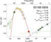 |
Fig. 6. SED fit for 00188−0856 as an example. The data points correspond to the radio (green diamonds), ALMA ∼220 GHz from this paper (red circle), and IR (remaining points) observations. The solid green line is the 5–38 μm Spitzer/IRS spectrum. The IR observations are color coded as follows: Spitzer/IRS synthetic photometry at 34 μm (green circle); Spitzer/MIPS (yellow circles); and Herschel/SPIRE (green triangles). The solid red line is the best gray-body fit and the dashed blue line represents the best power-law fit to the nonthermal radio emission. Only the encircled symbols have been used for the fits (i.e., the ALMA point is excluded from the SED fit). The dot-dashed green line represents the expected maximum free–free emission assuming that all the LIR is produced by SF (see Sect. 4.4). The SED fits for the whole sample are shown in Fig. D.1. |
IR and radio SED fit results
4.4.2. Nonthermal synchrotron emission
At the frequency of the ALMA observations, it is possible to have a significant contribution from nonthermal synchrotron emission. To estimate this contribution, we used published radio observations of our sample of ULIRGs with frequencies between 1 and 40 GHz (Table 5). All the systems have been observed at least at 1.4 GHz, except 13120−5453 which only has 4.85 and 0.843 GHz data. For objects with more than one radio observation (16 systems), we fit a power law to the radio data. We obtained spectral indexes between −0.3 and −1.0 with a mean index of −0.62 (see Table 6), which are similar to the spectral indexes found in a sample of 31 local ULIRGs by Clemens et al. (2008). For the remaining objects with just one radio observation at 1.4 GHz (9 systems), we assumed the mean spectral index between 1.4 and 22.5 GHz ( ) measured in local ULIRGs (Clemens et al. 2008). We find that the nonthermal emission contributes between 4 and 55% (median 20%) of the ALMA continuum flux (Table 6). In this fit, we ignored that the free–free emission (see below) can also affect (flatten) the spectral index (e.g., Hayashi et al. 2021). Therefore, if the free–free emission is strong compared to the synchrotron, our “nonthermal” contribution estimate would be closer to the combined free–free + synchrotron total emission.
For 20087−0308, the predicted nonthermal flux is 2.8 times higher than the observed ALMA flux. However, this source shows radio fluxes between 1.4 and 4.85 GHz that are not fully compatible with a power-law (Fig. D.1). This suggests that either the power-law model is not adequate for this source, that it presents variable radio emission, or that some of the radio fluxes are not reliable.
4.4.3. Free–free thermal emission
The ALMA continuum measurements can also include a contribution from thermal free–free emission. The free–free emission is related to the ionizing photon rate from young stars and can trace the star-formation rate (SFR; e.g., Condon & Ransom 2016). We used the relation between the SFR and the free–free radio emission to estimate its contribution at the ALMA frequency (Eq. (11) from Murphy et al. 2011). The SFR of the ULIRGs was derived from the total IR luminosity using the Kennicutt & Evans (2012) calibration. The free–free contributions are presented in Table 6. However, we note that this free–free emission estimate is an upper limit because we ignored the potential AGN contribution to the LIR, and also because, in the dusty nuclear regions of ULIRGs, a fraction of the ionizing photons can be absorbed by dust grains instead of ionizing H atoms and, therefore, reduce the actual free–free emission (e.g., Abel et al. 2009). Actually, with these assumptions, six systems (five classified as AGN and one as LINER) have predicted free–free upper limits above 90–100% of the observed ALMA flux. This indicates that a large part of their LIR likely comes from an AGN and it cannot be directly translated into SFR and subsequently into free–free emission.
5. Discussion
5.1. ALMA continuum as tracer of the IR luminosity
We aim to determine the physical size and luminosity surface density of the regions that emit the bulk of the IR luminosity in local ULIRGs. Far-IR telescopes, that detect the peak of the IR emission, lack the angular resolution to spatially resolve it, although it is possible to infer the size of the far-IR emission through indirect methods like the modeling of far-IR OH absorptions (e.g., González-Alfonso et al. 2015). In this section, we investigate if the ∼220 GHz ALMA continuum, which provides much higher angular resolutions, can be used as a proxy of the IR emission to obtain direct estimates of the IR emitting region sizes.
However, using the ∼220 GHz continuum to trace the size of ULIRGs is not straightforward. At this frequency, the continuum includes emission from dust, which is connected to the IR luminosity, but it may also include contributions from free–free and synchrotron emissions (Condon & Ransom 2016), which might not be directly related to the IR luminosity. This is important because, even if the IR luminosity of local ULIRGs is thought to be dominated by SF, the AGN contribution increases with increasing LIR (Veilleux et al. 2009; Nardini et al. 2009), and the synchrotron AGN emission could affect the ∼220 GHz source sizes. In addition, ALMA is an interferometer, so part of the emission might be filtered out. In this section, we study the impact of these effects on the measured source sizes.
5.1.1. Filtered out flux
In general, due to the limited coverage of the uv plane, interferometric observations filter out extended large scale emission. Therefore, it might be possible that extended continuum emission from our ULIRGs is missing in the measured fluxes (Sect. 4.1). To evaluate this possibility we compare the maximum recoverable scale of our observations (about 4 kpc; Sect. 3.1) with the sizes of the detected sources. The radii range from < 60 to 300 pc (Sect. 4.1 and Table 3), which are ≪4 kpc. If > 4 kpc structures were actually present in these ULIRGs, we would expect to detect, in addition to these very compact sources, intermediate size structures (∼2 kpc FHWM) which are not seen in the continuum images. This suggests that the 220 GHz continuum of ULIRGs is intrinsically compact and that we can recover most of the continuum emission with these data.
It also possible that we do not detect extended low-surface brightness continuum emission due to the observations sensitivity. To quantify its possible impact, we assume an emitting area with a 4 × 4 kpc2 size (the typical Hα effective radius of ULIRGs is < 2 kpc; Arribas et al. 2012). From the continuum sensitivity, Table 2, we estimated extended emission 3σ upper limits which are on average 8% of the measured fluxes and up to 20–75% for the four faint nuclei with f220 GHz < 0.7 mJy (F10190+1322 W; 11095−0238 SW, F12112+0305 SW, and 16155+0146 NW; see Table 3). Therefore, if low-surface brightness emission is present, its contribution would be small for the great majority of the nuclei (at least for 25 out of 29).
5.1.2. Dust, free–free, and synchrotron contributions
At the frequencies of the ALMA observations (190–250 GHz), in addition to the Rayleigh–Jeans tail of the IR dust emission, a contribution from thermal free–free, and nonthermal synchrotron emission is possible. In particular, we explore whether the free–free or synchrotron emissions could bias the measured sizes toward more compact sizes in the case of a starburst nucleus.
Dust. We first estimate the dust contribution. Based on the IR SED modeling (Sect. 4.4), we found that the ALMA flux densities are just slightly lower than the extrapolation of the IR gray-body fit (median ratio of 1.14; Table 6). We note that we did not use the ALMA flux in the gray-body fit. Thus, a possible interpretation for the good agreement between the data and the model prediction is that the ALMA flux comes from the long-wavelength tail of the dust gray-body emission. If this is the case, we could use the high-resolution ALMA data to determine the size of the IR emitting regions. This good agreement between the ALMA continuum flux and the IR SED extrapolation was also found by Imanishi et al. (2019) using 260 GHz observations of local ULIRGs at comparable spatial resolutions.
Free–free. The ALMA emission can include free–free emission as well. The free–free emission is produced by ionized hydrogen usually associated with star-forming regions (see Sect. 4.4.1). We estimated an upper limit for the free–free emission assuming that all the LIR is produced by SF (i.e., ignoring the possible AGN contribution). This assumption also implies that dust does not absorb any ionizing photon (Sect. 4.4.1). The upper limit for the free–free contribution has a median value of < 65% (Table 6). But even if the free–free emission dominates the ALMA flux, it should not affect the region size estimates since, for this free–free upper limit estimation, both IR and free–free emissions should be cospatial as they have a common star formation origin. Moreover, taking into account the AGN contribution to the LIR and the effect of absorption of UV photons by dust would reduce this upper limit and, therefore, the possible impact of the free–free emission on the source size measurements.
Synchrotron. Some contribution from synchrotron emission is possible too. If this synchrotron emission is produced by supernovae (i.e., related to star-forming regions), the ALMA regions sizes should not be affected since the IR emission and the supernovae (SNe) should have similar spatial distributions. Alternatively, AGN can produce strong synchrotron emission. In our sample, only F13451+1232 (4C+12.50) has excess radio emission with respect to the radio-IR relation (see Perna et al. 2021). Actually, the F13451+1232 ∼220 GHz emission is dominated by synchrotron radiation (see Fig. D.1) and, therefore, cannot be directly used as a proxy of the IR emitting region. For the remaining objects, we estimated a median nonthermal contribution, which includes both SNe and AGN emission, of 20% and up to 40–60% in four objects: one of the starbursts (09022−3615), one LINER (11095−0238), and two out of the seven systems classified as AGN in the optical (13120−5453, and 16155+0146). The latter suggests that the optical detection of an AGN does not imply that the ∼220 GHz emission is always dominated by synchrotron AGN emission in local ULIRGs. However, how the AGN synchrotron emission affects the ALMA source sizes is unclear. AGN jets producing synchrotron emission have sizes ranging from parsecs to few kiloparsecs in radio-quiet AGN (Hardcastle & Croston 2020). For instance, the synchrotron radio jet emission from the AGN ULIRG 01572+0009 (PG 0157+001) has a ∼7 kpc diameter (Leipski et al. 2006), although according to our SED modeling, the synchrotron contribution at 220 GHz is small, about 0.15, and should not affect the estimated size in this object. For the five systems with a high nonthermal contribution, we find that their sizes and luminosity and molecular gas surface densities do not differ from those of the rest of the sample (see Fig. 2).
5.1.3. Summary
It seems likely that these ∼220 GHz continuum ALMA observations trace the IR emitting region for the majority of local ULIRGs and that the filtered out flux due to the interferometric observations is small. The good agreement between the IR gray-body extrapolation and the ALMA fluxes supports this. Free-free and SNe synchrotron emissions could contribute to the ALMA flux, but since they have a star formation origin they should not affect the size estimates for a starburst ULIRG. Synchrotron emission from AGN could bias the size measurements, although we do not find significant differences in size between the five systems with high synchrotron emission and the rest of the sample. Therefore, in the following sections we assume that the size of the ∼220 GHz continuum is equivalent to the size of the region which emits the bulk of the IR luminosity in these ULIRGs.
5.2. Extreme nuclear IR luminosity densities
Using the half-light radius, rcont, of the ALMA continuum and half of the IR luminosity (Sects. 4.1 and 4.4), we calculated the luminosity surface density, ΣLIR, in the nuclear regions of the ULIRGs. For systems with two nuclei, we estimated their IR luminosity fraction using their relative ALMA continuum fluxes. In 70% of the interacting systems, the luminosity is completely dominated (>90% of the total luminosity) by one of the nuclei. These fractions and the resulting surface densities are listed in Table 7. We find log ΣLIR/(L⊙ kpc−2) between 11.5 and 14.3 with a median value of 13.2. If this IR luminosity is produced by SF, it corresponds to ΣSFR = 2500 M⊙ yr−1 kpc−2 using the Kennicutt & Evans (2012) SFR calibration. These values are much higher (1–2 orders of magnitude) than the densities found in local starburst LIRGs, even when they are observed at higher angular resolutions of ∼100 pc (e.g., Xu et al. 2015; Pereira-Santaella et al. 2016; Michiyama et al. 2020). Similarly, z ∼ 3–6 submillimeter galaxies have lower surface densities, 150–1300 M⊙ yr−1 kpc−2 when observed at ∼kpc resolutions (e.g., Riechers et al. 2017; Gómez-Guijarro et al. 2018). At higher resolutions, ∼200 pc, these submillimeter galaxies have ΣSFR between 100 and 3000 M⊙ yr−1 kpc−2 which are still lower than the majority of the local ULIRGs (e.g., Oteo et al. 2017; Gullberg et al. 2018).
Nuclear properties.
The observed ΣLIR range is comparable to that measured in local ULIRGs using radio and IR observations at similar angular resolution. Using 33 GHz radio data, Barcos-Muñoz et al. (2017) found a median surface density of 1012.8 L⊙ kpc−2 in a sample of 22 local interacting and merging systems with log LIR/L⊙ > 11.6. Similarly, González-Alfonso et al. (2015) estimated nuclear ΣLIR > 1012.8 L⊙ kpc−2 for ten local ULIRGs based on the modeling of the far-IR OH absorptions. In addition, mid-IR ground-based studies of ULIRGs derive maximum luminosity densities between 1012.1 and 1014.6 L⊙ kpc−2 (Soifer et al. 2000; Imanishi et al. 2011). For the western nucleus of F15327+2340 (Arp 220 W), using higher resolution data (<50 pc) a luminosity density about 1014.3−15.5 L⊙ kpc−2 has been estimated (Downes & Eckart 2007; Wilson et al. 2014; Sakamoto et al. 2017; González-Alfonso & Sakamoto 2019). Therefore, our results are compatible with previous findings and confirm that the luminosity density in the nucleus of local ULIRGs is much higher than in other local and high-z starbursts when measured at 100–1000 pc scales. To investigate the origin of this high ΣLIR values, we discuss two alternatives: an optically thick starburst and the presence of an obscured AGN.
5.2.1. Optically thick starburst
In Fig. 7, we plot the ΣLIR vs. ΣH2 (Sect. 4.3) relation for our sample of local ULIRGs. Based on theoretical models, a ΣLIR of ∼1013 L⊙ kpc−2 has been suggested as the maximum ΣLIR of warm (T < 200 K) optically thick starbursts (Thompson et al. 2005). The maximum ΣLIR for these warm starbursts is similar to the median value found in our sample. Hot (T > 200 K) optically thick starbursts could have ΣLIR ∼ 1015 L⊙ kpc−2 when ΣH2 > 106 M⊙ pc−2 (Andrews & Thompson 2011). However, we measure ΣH2 ≪ 106 M⊙ pc−2, so these local ULIRGs might be more similar to the warm optically thick starburst models.
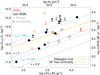 |
Fig. 7. Cold molecular gas surface density (ΣH2) vs. IR luminosity surface density (ΣLIR). Galaxy symbols are as in Fig. 5. The dotted black lines indicate the maximum luminosity from an instantaneous starburst using 100% (ϵ = 1) or 20% (ϵ = 0.2) of the available cold molecular gas (see Sect. 5.2.1). The orange solid line is the Eddington luminosity limit. For points above this line, the radiation pressure is stronger than gravity (Sect. 5.5). The dashed blue lines indicate the 1 and 10 Myr depletion times for reference assuming that the IR luminosity is produced by SF. The column density (NH) axis is calculated from ΣH2 assuming a uniform mass distribution (i.e., NH = 2 × ΣH2/m(H2) where m(H2) is the H2 molecular weight). |
Although the ΣLIR are similar to the maximum for a warm optically thick starburst, when combined with the ΣH2, the resulting depletion times, ΣH2/ΣSFR, would be shorter (<1–15 Myr; see Table 7) than those measured in other LIRG starbursts (>30–100 Myr; Xu et al. 2015; Pereira-Santaella et al. 2016).
We also estimated the maximum ΣLIR that a starburst can produce for a given ΣH2. Using STARBURST99 (Leitherer et al. 1999), we find that the maximum luminosity produced by a solar metallicity instantaneous burst, assuming a Kroupa (2001) initial mass function (IMF), is ∼1060 L⊙  at an age of ∼2.2 Myr (see also Sakamoto et al. 2013). In Fig. 7, we show this limit (ϵ = 1 dotted black line). This limit assumes that all the molecular gas is instantaneously transformed into stars (i.e., 100% efficient SF). In reality, stellar feedback dissipates the molecular clouds before a 100% efficiency is achieved, so the maximum luminosity from a starburst would be lower than this limit. Based on magneto-hydrodynamic simulations, the maximum efficiency per free-fall time is about 20% (e.g., Padoan et al. 2012) which is shown in Fig. 7 too (ϵ = 0.2). This figure shows that 70% of the nuclei are above the 100% efficiency limit (ϵ = 1) and all of them are above this 20% efficiency limit.
In addition, if the nuclear luminosity is produced by a compact and intense starburst, a continuous supply of molecular gas to the nucleus would be required to sustain the ongoing SFR level. Otherwise, it would not be possible to achieve the observed ΣLIR which implies depletion times < 1 Myr in 30% of the sample and < 15 Myr in all of them. However, the high radiation pressure in the nucleus, which is compatible with being above the Eddington limit for 67% of the nuclei (see Sect. 5.5), could prevent these massive gas inflows.
5.2.2. Obscured AGN
We find that 70% of the ULIRGs have ΣLIR/ΣH2 ratios above the limit for a ϵ = 1 efficient starburst. Also, 65% have ΣLIR above the theoretical value of an optically thick warm starburst (∼1013 L⊙ kpc−2). These fractions are similar for systems optically classified as AGN and starbursts (see Fig. 7). These results suggest that what produces the bulk of the IR luminosity in these local ULIRGs is not a standard starburst.
Alternatively, an AGN could dominate the LIR of these objects. This possibility has also been suggested because of the high ΣLIR in the ULIRG nuclei derived from mid-IR data (e.g., Imanishi et al. 2011) or from the millimeter continuum in Arp 220 (e.g., Downes & Eckart 2007; Wilson et al. 2014; Scoville et al. 2017; Sakamoto et al. 2017). From ΣH2, we estimate that the nuclear H column densities are moderate, between 1023 and 1024 cm−2 (see Fig. 7). These values are lower than the Compton thick limit (∼2 × 1024 cm−2), so we would expect the AGN X-ray emission not to be completely absorbed. Iwasawa et al. (2011) observed a sample of local U/LIRGs with Chandra at 0.5–7 keV. Twelve out of our 25 systems are part of their sample. They found AGN evidence in six out of the 12, but they estimated low AGN contributions to the LIR (3–20%). However, it is possible that the actual NH that obscures these AGN is actually higher and could absorb the 0.5–7 keV X-ray emission. Our NH estimates are based on molecular gas observations at ∼400 pc resolution, but the obscuring molecular torus could be smaller, as observed in local Seyfert galaxies (median diameter of 40 pc; Garcia-Burillo et al. 2021), so our NH values might be underestimated.
To minimize the effects of the obscuring column density, we also considered the Swift-BAT 105-Month 14–195 keV survey (Oh et al. 2018). This higher energy X-ray band is less affected by NH than the Chandra 0.5–7 keV range. The 5σ sensitivity of the survey is 8.4 × 10⁻¹² erg s−1 cm−2. Only one source in our sample, F05189−2524, is detected at 14–195 keV. For the rest of the targets, the Swift-BAT survey implies L14−195 keV < 1043.3−44.8 erg s−1, depending on the distance. Assuming that the bolometric AGN luminosity is LAGN ∼ 12 × L14−195 keV (Marconi et al. 2004), the 5σ upper limits would correspond to LAGN < 1044.3−45.9 erg s−1 = 1010.7−12.3 L⊙. This would result in an AGN contribution LAGN/LIR < 0.45 for all but one of these ULIRGs and a median upper limit of < 0.25. More sensitive NuSTAR > 10 keV observations were presented by Teng et al. (2015). Their sample contains four of our ULIRGs, three of them already classified as Sy in the optical. One is undetected (F14378−3651), in F15327+2340 (Arp 220) no AGN evidence is found, although a very deeply buried AGN is still possible, and F05189−2524 and 13120−5453 are Compton-thin and -thick AGN, respectively.
ULIRGs are known to be hard X-ray underluminous (Imanishi & Terashima 2004; Teng et al. 2015) and AGN in mergers are also heavily obscured (Ricci et al. 2017). The combination of these two factors could explain why the AGN in these sources, if present, remain mostly undetected in X-ray observations.
As discussed before, the high ΣLIR/ΣH2 nuclear ratios cannot be easily explained by a starburst, even if an optically thick one is considered. These ALMA data would be consistent with an AGN dominating the IR luminosity, but it is not possible to confirm that an AGN is present in the nuclei of the majority of these ULIRGs. The nondetection of these possible AGN in ultra-hard X-ray observations could indicate extremely high obscuring column densities. Higher angular resolution ALMA data could spatially resolve the obscuring material and establish its actual column density as in nearby Seyfert galaxies (e.g., Garcia-Burillo et al. 2021).
5.2.3. Systematic uncertainties
There are several assumptions which could bias the ΣLIR and ΣH2 values presented in Fig. 7. For instance, the rCO size used to estimate the nuclear ΣH2 is larger than the rcont used for ΣLIR. This is because the CO(2–1) emission is more extended than the ∼220 GHz continuum (rCO/rcont = 2.5 ± 1.1; see Sect. 4.3) and it is not possible to exactly determine the amount of CO(2–1) within the rcont region since, in most cases, both rcont and rCO are smaller than the beam size. Therefore, ΣH2 are averaged over larger regions than ΣLIR and the true nuclear ΣH2 could be higher. Consequently, the real star formation efficiency (depletion time) could be lower (longer). Actually, González-Alfonso et al. (2015), by modeling the far-IR OH absorptions, estimated nuclear ΣH2 between 103.8 and 104.7 M⊙ pc−2 for ten local ULIRGs. These values are ∼5 times higher than our average ΣH2 derived from CO(2–1) using ∼400 pc resolution data. In addition, eight of our targets are part of a survey to detect vibrationally excited HCN emission to identify compact obscured nuclei (CONs). The HCN-vib (3–2) 267.199 GHz line is detected in five of these systems (63 ± 18%; see Table 7 and Imanishi et al. 2016, 2019; Falstad et al. 2021). Similarly, the mid-IR HCN-vib 14 μm absorption, which populates the levels originating the HCN-vib emission, is detected in ten (six interacting systems and four mergers) out of the 23 systems (43 ± 10% globally, 60 ± 15% of the interacting systems and 31 ± 13% of the advanced mergers; Table 7). The presence of these HCN-vib spectral features suggests the presence of extreme nuclear column densities too. Higher resolution CO(2–1) data will help us to establish the cold molecular gas column density more accurately. The already available high resolution CO(2–1) data for 17208−0014 (120 pc resolution; see Sect. 4.2), suggest a factor of 2 higher nuclear ΣH2 (Pereira-Santaella, in prep.). However, for this galaxy, the nuclear ΣLIR also increases by a factor of ∼5 using these data, so the resulting ΣSFR/ΣH2 ratio would be even higher and reinforce the need for an obscured AGN in this object.
Another uncertainty related to the ΣH2 is the αCO conversion factor. We assumed a ULIRG-like factor, which is relatively low compared to the conversion factor used for normal galaxies (see e.g., Bolatto et al. 2013). High nuclear column densities can produce self-absorbed CO(2–1) line profiles as seen in the compact nuclei of some local LIRGs (e.g., Sakamoto et al. 2013; Pereira-Santaella et al. 2017; González-Alfonso et al. 2021). If the nuclear CO(2–1) emission of these ULIRGs is self-absorbed, the assumed ULIRG-like αCO conversion factor could result in underestimated ΣH2 values. For this paper, we opt to use the standard ULIRG-like αCO, as it is typically done in local ULIRG studies, but we will investigate the presence of self-absorbed CO(2–1) profiles in these targets in a future paper. The depletion times depend on the assumed αCO conversion factor. If the actual αCO of these objects is similar to the Milky Way factor (i.e., 5 times higher; Bolatto et al. 2013), the molecular gas mass will be 5 times higher, and the depletion times 5 times longer. However, the median tdep would still be very short (<6 Myr).
Finally, the maximum luminosity for a starburst (dotted lines in Fig. 7) is calculated using a Kroupa (2001) IMF. If the IMF in ULIRGs is top-heavy as suggested by some works (see e.g., Sliwa et al. 2017; Brown & Wilson 2019), the maximum starburst luminosity per unit of molecular gas could be higher. For example, the maximum luminosity for an IMF truncated at 30 M⊙ would produce ∼10 times more luminosity per unit of molecular gas than the standard Kroupa (2001) IMF. For an ϵ = 0.2 efficiency, this top-heavy IMF could explain the ΣLIR/ΣH2 ratios observed in about half of the nuclei, although these starbursts would have radiation pressures above the Eddington limit and they would not be stable on short timescales of few Myr (see Sect. 5.5).
5.3. Continuum and CO(2–1) sizes versus mid-IR excess
In the left panel of Fig. 8, we show the relation between the excess mid-IR emission (Sect. 4.4.1) and the 220 GHz continuum size, rcont. We note that the excess mid-IR emission is estimated from the system integrated Spitzer/IRS spectra. Therefore, in interacting systems where a nuclei dominates the total LIR, the mid-IR excess of the secondary nucleus cannot be directly estimated from this integrated spectrum. Thus, we excluded the eight nuclei in interacting systems with IR luminosity fractions < 20% (see Table 7). In this diagram, we can classify the ULIRG nuclei in two main groups: compact objects (rcont < 120 pc) with high mid-IR excess (logarithm > − 0.9; red box); and objects following a linear relationship between the two properties with decreasing excess mid-IR emission for decreasing rcont (blue line).
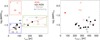 |
Fig. 8. Logarithm of the excess mid-IR emission vs. size of the 220 GHz continuum (left panel) and size of the CO(2–1) emission (right panel). Galaxy symbols are as in Fig. 5. The solid orange line is the best linear fit to the non-AGN (black) points. In the left panel, the red box (a) marks a region of this diagram solely occupied by optically detected AGN. The blue box (b) indicates the location of very compact ULIRG nuclei (mostly unresolved by our data) with negligible excess mid-IR emission. The green box shows the location of more extended nuclei with higher mid-IR excess. |
The first group exclusively contains objects classified as AGN in the optical. We note that the two interacting systems in our sample with no ALMA data, F12072−0444 and F13451+1232, are optical AGN with log ΔL6−20 μm/LIR > −0.9 and could lie in this region of the diagram as well. The location of these AGN in this diagram (red box) is what is expected if warm dust (which emits in the mid-IR) from a compact torus produces a significant part of their total LIR. Actually, the mid-IR f15 μm/f30 μm color, which behaves similar to the mid-IR excess, have been used to estimate the AGN luminosity contribution in ULIRGs (e.g., Veilleux et al. 2009).
For the remaining nuclei there is a correlation (rs = 0.87 and p = 1 × 10⁻³) between the continuum size and the mid-IR excess with increasing sizes for increasing mid-IR excess emission. The size of these sources ranges from < 70 pc to ∼300 pc and the best linear fit is log ΔL6−20μm/LIR = (− 1.8 ± 0.1)+(2.2 ± 0.6)×10−3 × rcont/pc.
In Fig. 8 (left panel), we highlighted (blue box) sources with rcont < 120 pc. This box contains 46% of the sample (12 nuclei out of 26). They have sizes comparable to the AGN (red box), although most of them only have an upper limit rcont, so their real size could be lower than that of the AGN. Opposite to most AGN, which have excess mid-IR emission between 15 and 70% of the LIR, these objects have negligible mid-IR excess (<3%). A majority of the nuclei in interacting systems (60%) lie in this blue box while it only includes 30% of the mergers. Actually, mergers following this relation have larger radii (median 160 pc) than the interacting systems (median 90 pc). This suggests that during the early phases of the interaction (nuclear separation > 1 kpc), most of the activity (AGN and/or SF) occurs in compact regions where most of the mid-IR emission is absorbed by dust and then re-emitted in the far-IR. Then, in more advanced merger stages (nuclear separation < 1 kpc), the activity appears on more extended regions (green box in Fig. 8), unless an optically detected AGN is present (red box sources).
In Fig. 9, we indicate the systems with AGN contributions > 50% based on mid-IR observations (Veilleux et al. 2009; Nardini et al. 2010). The majority of the optical AGN are also classified as AGN by these mid-IR diagnostics (five out of seven) and only three non-Sy are identified as mid-IR AGN. In addition, this figure shows that there is a good correlation between the mid-IR AGN classification and the mid-IR excess. This is because these mid-IR diagnostics are based on the detection of warm dust which is closely related to the mid-IR excess definition used here. Therefore, if the mid-IR emission of the AGN in these ULIRGs is absorbed (see also Sect. 5.4), these mid-IR diagnostics could fail to detect them.
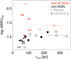 |
Fig. 9. Same as left panel of Fig. 8, but galaxies with more than 50% AGN contribution based on mid-IR observations are indicated in red (Veilleux et al. 2009; Nardini et al. 2010). |
The right panel of Fig. 8 shows the excess mid-IR emission as function of the molecular gas emission size rCO. We do not find a significant correlation between the molecular gas size and the mid-IR excess (rs = 0.34 and p = 0.12). The molecular gas emission size is similar in the interacting systems and advanced mergers (median ∼350 pc). On the contrary, hydrodynamic simulations predict that strong torques during the first passage can pile up the gas in ∼kpc-scale starbursts and later, during the final-coalescence, in more compact subkiloparsec starbursts (e.g., Hopkins et al. 2013).
We find that, for the interacting systems, the molecular gas and the continuum size distributions are very different (see Fig. 10). The radii of the molecular gas emission is uniformly distributed over the whole observed range (mostly between 200 and 500 pc; right panel of Fig. 10) while the continuum size distribution peaks at compact radii (<100 pc; left panel of Fig. 10). This suggests that, even if there is a global correlation between the continuum and the CO emission sizes for the whole sample of ULIRGs (see Sect. 4.3 and Fig. 2), for the interacting systems, the two sizes seem to be decoupled. An obscured AGN, which do not need large amounts of molecular gas to produce high luminosities, could explain why these interacting nuclei have very compact continuum sources but a more extended molecular gas distribution.
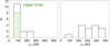 |
Fig. 10. Distribution of the 220 GHz continuum radius rcont (left) and the CO(2–1) emission radius rCO (right) for the nuclei in interacting ULIRGs. The upper limits for the 220 GHz continuum are included in the first bin and indicated by the green shaded area. |
5.4. Continuum size vs. silicate absorption and IR colors
In this section, we explore possible relations between the 220 GHz continuum size and other IR tracers. As in Sect. 5.3, we excluded from this analysis nuclei with contributions < 20% to the total IR luminosity of the systems. We first consider the 9.7 μm silicate absorption. We use the 9.7 μm silicate strengths from the Infrared Database of Extragalactic Observables from Spitzer (IDEOS; Table A.1; Hernán-Caballero et al. 2020; Spoon et al., in prep.). Deep silicate absorptions have been associated with an evolutionary phase in which the obscuring molecular cocoon created during the early interaction phases have not been yet shed (e.g., Spoon et al. 2007). Therefore, we could expect a relation between the silicate absorption and the size of the cold molecular or dust continuum emissions. However, we find no significant correlation between them (see left and middle panels of Fig. 11). To explain this absence of correlation, we argue that to measure deep 9.7 μm silicate absorption, some mid-IR radiation must escape the nuclear molecular cocoon. As shown in Sect. 5.3, the fraction of the total IR emission that is emitted in the mid-IR is greatly reduced in the most compact nuclei (i.e., the mid-IR emission is absorbed and then re-emitted in the far-IR). Therefore, the 9.7 μm silicate absorption is not necessarily extreme in these compact sources since their nuclear mid-IR emission is possibly absorbed and what is observed in the mid-IR is likely produced by less obscured external regions. The presence of several CONs in our sample (see Falstad et al. 2021), is also consistent with the mid-IR emission of the hot nucleus being obscured. Likewise, ground-based mid-IR spectroscopy of local AGN ULIRGs showed that their silicate absorptions are produced by dust not directly associated with the AGN (Alonso-Herrero et al. 2016). This scenario is also supported by radiative transfer models of compact nuclei where the mid-IR emission is completely absorbed for objects with very high column densities (NH2 > 1025 cm−2; see Fig. 2 of González-Alfonso & Sakamoto 2019).
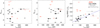 |
Fig. 11. Relation between the 9.7 μm silicate absorption and the 220 GHz continuum (left) and the CO(2–1) (middle) sizes. Right panel: 220 GHz continuum size vs. IRAS 12 μm/25 μm color relation. Symbols as in Fig. 5. For the IRAS 12 μm/25 μm color relation (right), the best linear fit to the non-AGN objects (black symbols) is log f12/f25 = (− 1.29 ± 0.04)+(1.6 ± 0.3)×10−3 × rcont/pc. |
We also studied possible correlations between the broad-band IRAS colors and the size of the continuum and cold molecular emissions. Most of the ULIRGs are undetected by IRAS at 12 μm, for this reason we computed synthetic fluxes for the four IRAS bands (12, 25, 60, and 100 μm) form the Spitzer/IRS spectrum and the IR SED model (Sect. 4.4). We tried the 6 IRAS color combinations. Only the f12/f25 color shows a significant correlation with the continuum size (Fig. 11 right). The f12/f25 ratio is actually related to the mid-IR excess emission. The 12 μm flux would trace the mid-IR emission while at 25 μm, the emission is dominated by the IR gray-body for most of the non-AGN ULIRGs. Therefore, this relation would be equivalent to that presented in Sect. 5.3 with the mid-IR excess emission.
5.5. Nuclear radiation pressure. Eddington limit
We find very high ΣLIR in the nuclei of the ULIRGs, so it is important to determine if the radiation pressure can overcome the gravity attraction in these objects. To do so, we calculated the Eddington limit in the ΣH2 − ΣLIR plane by fitting the model results reported by González-Alfonso & Sakamoto (2019). These models assume spherical symmetry and accurately determine the force due to radiation pressure once the equilibrium Tdust profile across the source is calculated. The models assume a density profile ∼r−1, such that ΣH2 does not depend on the source radius. Our fitting, shown in Fig. 7 with an orange line, is approximately valid for ΣH2 ≲ 3 × 10⁴ M⊙ pc−2, and assumes an intermediate molecular gas fraction with respect to the total mass, fg = 0.3, and a gas-to-dust ratio of fgd = 100 by mass. In the optically thick limit, the Eddington luminosity is proportional to  (Andrews & Thompson 2011).
Figure 7 shows that half of the nuclei, 19 out of the 29, are above the estimated Eddington limit (see also Table 7). This suggests that the radiation pressure can be stronger than gravity in these nuclei and, therefore, massive gas outflows are expected. This result is consistent with the detection of massive molecular outflows in local ULIRGs (Sturm et al. 2011; Cicone et al. 2014; González-Alfonso et al. 2017; Pereira-Santaella et al. 2018; Lutz et al. 2020) and also supports that radiation pressure plays a relevant role as a potential launching mechanism of the outflows in local ULIRGs.
6. Conclusions
We have analyzed new high-resolution ALMA ∼220 GHz and CO(2–1) observations of a representative sample of 23 local ULIRGs (34 individual nuclei) as part of the Physics of ULIRGs with MUSE and ALMA (PUMA) project (see also Perna et al. 2021). The main results of this work are the following:
-
We modeled the ∼220 GHz (190–250 GHz) continuum emission of these ULIRGs. We find that the median deconvolved half light radius (rcont) is 80–100 pc and about 40% (11/29 with continuum detection) of the nuclei are not resolved by these data. From the IR and radio SED modeling, we obtain that the ALMA ∼220 GHz continuum fluxes are in good agreement, within a factor of 2 (median ratio of 1.1 ± 0.7), with the extrapolation of the dust far-IR gray body emission. This suggests that the ∼220 GHz continuum traces the regions emitting the bulk of the IR luminosity in these objects. We estimate that the contributions from synchrotron (∼20%) and free–free emission (<65%) to the ALMA flux are not likely to bias the measured sizes. Using the ∼220 GHz continuum size, we calculate IR luminosity densities, ΣLIR, in the range 1011.5 − 1014.3 L⊙ kpc−2 (median 1013.2 L⊙ kpc−2), which is equivalent to ΣSFR = 2500 M⊙ yr−1 kpc−2. This is similar to the range derived from previous radio and ground-based mid-IR observations and 1–2 orders of magnitude brighter than local and high-z starbursts.
-
Similarly, we measure deconvolved CO(2–1) emission sizes, rCO, between 60 and 700 pc. These are on average 2.5 ± 1.1 times larger than the ∼220 GHz continuum size. We find no differences between systems optically classified as AGN or starburst or between interacting systems and advanced mergers. Using a ULIRG-like αCO conversion factor, we find nuclear molecular gas surface densities, ΣH2, in the range 102.9 − 104.2 M⊙ pc−2.
-
If the LIR is produced by SF, the ΣLIR/ΣH2 ratios imply extremely short molecular gas depletion times (<1–15 Myr). In addition, 70% of the nuclei would have SF efficiencies above the maximum for a starburst (ϵ = 1) and all of them would have ϵ > 0.2, which is the maximum efficiency per free-fall time predicted by simulations. These findings suggests that the bulk of the IR luminosity of these ULIRGs does not originate in a nuclear starburst. An obscured AGN with LAGN/LIR > 0.5 would be an alternative energy source.
-
For the compact nuclei (rcont < 120 pc) in interacting system with low mid-IR excess emission, the rcont is not correlated with the cold molecular gas emission, rCO, which varies between 200 and 500 pc. This could support the presence of a deeply embedded AGN which, opposed to star formation, would not require large amounts of cold molecular gas to produce the observed high IR luminosities.
-
The presence of compact and extremely embedded nuclei is supported by the detection of the HCN-vib 14 μm absorption in 43 ± 10% of the sample. The detection rate is higher, 60 ± 15%, in interacting systems than in advanced mergers, 31 ± 13%.
-
The ULIRG nuclei can be classified in two groups in the 220 GHz continuum size, rcont, vs. mid-IR excess emission, ΔL6−20 μm, diagram. ΔL6−20 μm is the 6–20 μm emission excess after subtracting the far-IR gray-body contribution in this wavelength range. These two groups are: (a) compact (rcont< 120 pc) nuclei with high mid-IR excess emission (log ΔL6−20 μm/LIR > −0.9) which are optically classified AGN; and (b) objects that follow a relation with decreasing rcont for decreasing mid-IR excess emission. A majority of the nuclei in interacting systems (60%) that follow this relation have rcont < 120 pc, which are at the lower end of the rcont–mid-IR excess relation, while only 30% of the mergers have these compact continuum emission. Mergers following this relation have larger sizes on average. This suggest that in the early stages of the interaction (nuclear separation > 1 kpc) most of the activity occurs in very compact regions while, in more advanced merger stages, the activity is more extended unless and optically detected AGN is present.
-
We find no correlation between the 9.7 μm silicate absorption and the ∼220 GHz continuum or CO(2–1) sizes. The relatively faint mid-IR emission of the most compact nuclei could prevent the presence of deep silicate absorptions in their mid-IR spectra and this could hinder the use of this absorption feature to find some obscured nuclei.
-
We find that 67% (19/29) of the nuclei have nuclear radiation pressures above the estimated Eddington limit. This is consistent with the presence of massive molecular outflows in ULIRGs and supports that radiation pressure can have a relevant role in the outflow launching process.
Acknowledgments
We thank the referee for the useful comments and suggestions. We are grateful to A. Hernán-Caballero and H. Spoon for providing measurements from the IDEOS database. MPS and IL acknowledge support from the Comunidad de Madrid through the Atracción de Talento Investigador Grant 2018-T1/TIC-11035 and PID2019-105423GA-I00 (MCIU/AEI/FEDER,UE). AA-H and SG-B acknowledge support through grant PGC2018-094671-B-I00 (MCIU/AEI/FEDER,UE). MP is supported by the Programa Atracción de Talento de la Comunidad de Madrid via grant 2018-T2/TIC-11715. AL acknowledges the support from Comunidad de Madrid through the Atracción de Talento Investigador Grant 2017-T1/TIC-5213. SA, LC, MP, and AL acknowledge support from the Spanish Ministerio de Economía y Competitividad through grants ESP2017-83197-P and PID2019-106280GB-I00. This work was done under project No. MDM-2017-0737 Unidad de Excelencia “María de Maeztu”- Centro de Astrobiología (INTA-CSIC). D. Rigopoulou acknowledges support from STFC through grant ST/S000488/1. This paper makes use of the following ALMA data: ADS/JAO.ALMA#2015.1.00113.S, ADS/JAO.ALMA#2015.1.00263.S, ADS/JAO.ALMA#2016.1.00170.S, ADS/JAO.ALMA#2016.1.00777.S, ADS/JAO.ALMA#2018.1.00486.S, and ADS/JAO.ALMA#2018.1.00699.S. ALMA is a partnership of ESO (representing its member states), NSF (USA) and NINS (Japan), together with NRC (Canada) and NSC and ASIAA (Taiwan) and KASI (Republic of Korea), in cooperation with the Republic of Chile. The Joint ALMA Observatory is operated by ESO, AUI/NRAO and NAOJ. The National Radio Astronomy Observatory is a facility of the National Science Foundation operated under cooperative agreement by Associated Universities, Inc.
References
- Abel, N. P., Dudley, C., Fischer, J., Satyapal, S., & van Hoof, P. A. M. 2009, ApJ, 701, 1147 [NASA ADS] [CrossRef] [Google Scholar]
- Alonso-Herrero, A., Ramos Almeida, C., Esquej, P., et al. 2014, MNRAS, 443, 2766 [NASA ADS] [CrossRef] [Google Scholar]
- Alonso-Herrero, A., Esquej, P., Roche, P. F., et al. 2016, MNRAS, 455, 563 [NASA ADS] [CrossRef] [Google Scholar]
- Andrews, B. H., & Thompson, T. A. 2011, ApJ, 727, 97 [NASA ADS] [CrossRef] [Google Scholar]
- Arribas, S., Colina, L., Alonso-Herrero, A., et al. 2012, A&A, 541, A20 [NASA ADS] [CrossRef] [EDP Sciences] [Google Scholar]
- Baan, W. A., & Klöckner, H.-R. 2006, A&A, 449, 559 [NASA ADS] [CrossRef] [EDP Sciences] [Google Scholar]
- Barcos-Muñoz, L., Leroy, A. K., Evans, A. S., et al. 2015, ApJ, 799, 10 [Google Scholar]
- Barcos-Muñoz, L., Leroy, A. K., Evans, A. S., et al. 2017, ApJ, 843, 117 [NASA ADS] [CrossRef] [Google Scholar]
- Barvainis, R., & Antonucci, R. 1989, ApJS, 70, 257 [NASA ADS] [CrossRef] [Google Scholar]
- Bolatto, A. D., Wolfire, M., & Leroy, A. K. 2013, ARA&A, 51, 207 [Google Scholar]
- Brown, T., & Wilson, C. D. 2019, ApJ, 879, 17 [NASA ADS] [CrossRef] [Google Scholar]
- Casey, C. M., Narayanan, D., & Cooray, A. 2014, Phys. Rep., 541, 45 [Google Scholar]
- Chu, J. K., Sanders, D. B., Larson, K. L., et al. 2017, ApJS, 229, 25 [Google Scholar]
- Cicone, C., Maiolino, R., Sturm, E., et al. 2014, A&A, 562, A21 [NASA ADS] [CrossRef] [EDP Sciences] [Google Scholar]
- Clemens, M. S., Vega, O., Bressan, A., et al. 2008, A&A, 477, 95 [NASA ADS] [CrossRef] [EDP Sciences] [Google Scholar]
- Condon, J. J., & Ransom, S. M. 2016, Essential Radio Astronomy (Princeton, NJ: Princeton University Press) [Google Scholar]
- Condon, J. J., Helou, G., Sanders, D. B., & Soifer, B. T. 1990, ApJS, 73, 359 [NASA ADS] [CrossRef] [Google Scholar]
- Condon, J. J., Huang, Z. P., Yin, Q. F., & Thuan, T. X. 1991, ApJ, 378, 65 [NASA ADS] [CrossRef] [Google Scholar]
- Condon, J. J., Helou, G., Sanders, D. B., & Soifer, B. T. 1996, ApJS, 103, 81 [NASA ADS] [CrossRef] [Google Scholar]
- Condon, J. J., Cotton, W. D., Greisen, E. W., et al. 1998, AJ, 115, 1693 [NASA ADS] [CrossRef] [Google Scholar]
- Díaz-Santos, T., Charmandaris, V., Armus, L., et al. 2010, ApJ, 723, 993 [Google Scholar]
- Downes, D., & Eckart, A. 2007, A&A, 468, L57 [NASA ADS] [CrossRef] [EDP Sciences] [Google Scholar]
- Duc, P. A., Mirabel, I. F., & Maza, J. 1997, A&AS, 124, 533 [NASA ADS] [CrossRef] [EDP Sciences] [Google Scholar]
- Falstad, N., Aalto, S., König, S., et al. 2021, A&A, 649, A105 [CrossRef] [EDP Sciences] [Google Scholar]
- Garcia-Burillo, S., Alonso-Herrero, A., Ramos Almeida, C., et al. 2021, A&A, submitted [arXiv:2104.10227] [Google Scholar]
- Genzel, R., Lutz, D., Sturm, E., et al. 1998, ApJ, 498, 579 [NASA ADS] [CrossRef] [Google Scholar]
- Gómez-Guijarro, C., Toft, S., Karim, A., et al. 2018, ApJ, 856, 121 [Google Scholar]
- González-Alfonso, E., & Sakamoto, K. 2019, ApJ, 882, 153 [NASA ADS] [CrossRef] [Google Scholar]
- González-Alfonso, E., Fischer, J., Sturm, E., et al. 2015, ApJ, 800, 69 [NASA ADS] [CrossRef] [Google Scholar]
- González-Alfonso, E., Fischer, J., Spoon, H. W. W., et al. 2017, ApJ, 836, 11 [NASA ADS] [CrossRef] [Google Scholar]
- González-Alfonso, E., Pereira-Santaella, M., Fischer, J., et al. 2021, A&A, 645, A49 [EDP Sciences] [Google Scholar]
- Gullberg, B., Swinbank, A. M., Smail, I., et al. 2018, ApJ, 859, 12 [NASA ADS] [CrossRef] [Google Scholar]
- Hardcastle, M. J., & Croston, J. H. 2020, New Astron. Rev., 88 [Google Scholar]
- Hayashi, T. J., Hagiwara, Y., & Imanishi, M. 2021, MNRAS, 504, 2675 [CrossRef] [Google Scholar]
- Helfand, D. J., White, R. L., & Becker, R. H. 2015, ApJ, 801, 26 [NASA ADS] [CrossRef] [Google Scholar]
- Hernán-Caballero, A., Spoon, H. W. W., Alonso-Herrero, A., et al. 2020, MNRAS, 497, 4614 [CrossRef] [Google Scholar]
- Hopkins, P. F., Cox, T. J., Hernquist, L., et al. 2013, MNRAS, 430, 1901 [Google Scholar]
- Houck, J. R., Roellig, T. L., van Cleve, J., et al. 2004, ApJS, 154, 18 [NASA ADS] [CrossRef] [Google Scholar]
- Imanishi, M., & Terashima, Y. 2004, AJ, 127, 758 [NASA ADS] [CrossRef] [Google Scholar]
- Imanishi, M., Imase, K., Oi, N., & Ichikawa, K. 2011, AJ, 141, 156 [CrossRef] [Google Scholar]
- Imanishi, M., Nakanishi, K., & Izumi, T. 2016, AJ, 152, 218 [NASA ADS] [CrossRef] [Google Scholar]
- Imanishi, M., Nakanishi, K., & Izumi, T. 2019, ApJS, 241, 19 [CrossRef] [Google Scholar]
- Imanishi, M., Kawamuro, T., Kikuta, S., Nakano, S., & Saito, Y. 2020, ApJ, 891, 140 [CrossRef] [Google Scholar]
- Iwasawa, K., Sanders, D. B., Teng, S. H., et al. 2011, A&A, 529, A106 [NASA ADS] [CrossRef] [EDP Sciences] [Google Scholar]
- Jiang, B. W., Gao, J., Omont, A., Schuller, F., & Simon, G. 2006, A&A, 446, 551 [NASA ADS] [CrossRef] [EDP Sciences] [Google Scholar]
- Kennicutt, R. C., & Evans, N. J. 2012, ARA&A, 50, 531 [NASA ADS] [CrossRef] [Google Scholar]
- Kim, D., Veilleux, S., & Sanders, D. B. 1998, ApJ, 508, 627 [NASA ADS] [CrossRef] [Google Scholar]
- Klaas, U., Haas, M., Müller, S. A. H., et al. 2001, A&A, 379, 823 [NASA ADS] [CrossRef] [EDP Sciences] [Google Scholar]
- Kovács, A., Omont, A., Beelen, A., et al. 2010, ApJ, 717, 29 [NASA ADS] [CrossRef] [Google Scholar]
- Kroupa, P. 2001, MNRAS, 322, 231 [NASA ADS] [CrossRef] [Google Scholar]
- Lahuis, F., Spoon, H. W. W., Tielens, A. G. G. M., et al. 2007, ApJ, 659, 296 [NASA ADS] [CrossRef] [Google Scholar]
- Lebouteiller, V., Barry, D. J., Spoon, H. W. W., et al. 2011, ApJS, 196, 8 [NASA ADS] [CrossRef] [Google Scholar]
- Leipski, C., Falcke, H., Bennert, N., & Hüttemeister, S. 2006, A&A, 455, 161 [NASA ADS] [CrossRef] [EDP Sciences] [Google Scholar]
- Leitherer, C., Schaerer, D., Goldader, J. D., et al. 1999, ApJS, 123, 3 [Google Scholar]
- Leroy, A. K., Evans, A. S., Momjian, E., et al. 2011, ApJ, 739, L25 [NASA ADS] [CrossRef] [Google Scholar]
- Lonsdale, C. J., Farrah, D., & Smith, H. E. 2006, in Ultraluminous Infrared Galaxies, ed. J. W. Mason (Berlin: Springer Verlag), 285 [Google Scholar]
- Lutz, D., Sturm, E., Janssen, A., et al. 2020, A&A, 633, A134 [NASA ADS] [CrossRef] [EDP Sciences] [Google Scholar]
- Marconi, A., Risaliti, G., Gilli, R., et al. 2004, MNRAS, 351, 169 [Google Scholar]
- Mauch, T., Murphy, T., Buttery, H. J., et al. 2003, MNRAS, 342, 1117 [NASA ADS] [CrossRef] [Google Scholar]
- Mcmullin, J. P., Waters, B., Schiebel, D., Young, W., & Golap, K. 2007, in Astronomical Data Analysis Software and Systems XVI, eds. R. A. Shaw, F. Hill, & D. J. Bell, ASP Conf. Ser., 376, 127 [Google Scholar]
- Meyers, B. W., Hurley-Walker, N., Hancock, P. J., et al. 2017, PASA, 34 [Google Scholar]
- Michiyama, T., Iono, D., Nakanishi, K., et al. 2020, ApJ, 895, 85 [Google Scholar]
- Moshir, M., Copan, G., Conrow, T. I. R. A. S., Source, Faint, et al. 1990, Catalogue [Google Scholar]
- Murphy, T., Mauch, T., Green, A., et al. 2007, MNRAS, 382, 382 [NASA ADS] [CrossRef] [Google Scholar]
- Murphy, E. J., Condon, J. J., Schinnerer, E., et al. 2011, ApJ, 737, 67 [NASA ADS] [CrossRef] [Google Scholar]
- Nagar, N. M., Wilson, A. S., Falcke, H., Veilleux, S., & Maiolino, R. 2003, A&A, 409, 115 [NASA ADS] [CrossRef] [EDP Sciences] [Google Scholar]
- Nardini, E., Risaliti, G., Salvati, M., et al. 2008, MNRAS, 385, L130 [NASA ADS] [Google Scholar]
- Nardini, E., Risaliti, G., Salvati, M., et al. 2009, MNRAS, 399, 1373 [Google Scholar]
- Nardini, E., Risaliti, G., Watabe, Y., Salvati, M., & Sani, E. 2010, MNRAS, 405, 2505 [NASA ADS] [Google Scholar]
- Oh, K., Koss, M., Markwardt, C. B., et al. 2018, ApJS, 235, 4 [Google Scholar]
- Oteo, I., Zwaan, M. A., Ivison, R. J., Smail, I., & Biggs, A. D. 2017, ApJ, 837, 182 [NASA ADS] [CrossRef] [Google Scholar]
- Padoan, P., Haugbølle, T., & Nordlund, Å. 2012, ApJ, 759, L27 [NASA ADS] [CrossRef] [MathSciNet] [Google Scholar]
- Pearson, C., Rigopoulou, D., Hurley, P., et al. 2016, ApJS, 227, 9 [Google Scholar]
- Pereira-Santaella, M., Colina, L., García-Burillo, S., et al. 2016, A&A, 587, A44 [NASA ADS] [CrossRef] [EDP Sciences] [Google Scholar]
- Pereira-Santaella, M., González-Alfonso, E., Usero, A., et al. 2017, A&A, 601, L3 [NASA ADS] [CrossRef] [EDP Sciences] [Google Scholar]
- Pereira-Santaella, M., Colina, L., García-Burillo, S., et al. 2018, A&A, 616, A171 [NASA ADS] [CrossRef] [EDP Sciences] [Google Scholar]
- Perna, M., Arribas, S., Catalán-Torrecilla, C., et al. 2020, A&A, 643, A139 [CrossRef] [EDP Sciences] [Google Scholar]
- Perna, M., Arribas, S., Pereira Santaella, M., et al. 2021, A&A, 646, A101 [EDP Sciences] [Google Scholar]
- Petric, A. O., Ho, L. C., Flagey, N. J. M., & Scoville, N. Z. 2015, ApJS, 219, 22 [Google Scholar]
- Planck Collaboration XXV. 2011, A&A, 536, A25 [NASA ADS] [CrossRef] [EDP Sciences] [Google Scholar]
- Ricci, C., Bauer, F. E., Treister, E., et al. 2017, MNRAS, 468, 1273 [NASA ADS] [Google Scholar]
- Riechers, D. A., Leung, T. K. D., Ivison, R. J., et al. 2017, ApJ, 850, 1 [Google Scholar]
- Rieke, G. H., Young, E. T., Engelbracht, C. W., et al. 2004, ApJS, 154, 25 [NASA ADS] [CrossRef] [Google Scholar]
- Sakamoto, K., Aalto, S., Costagliola, F., et al. 2013, ApJ, 764, 42 [NASA ADS] [CrossRef] [Google Scholar]
- Sakamoto, K., Aalto, S., Barcos-Muñoz, L., et al. 2017, ApJ, 849, 14 [NASA ADS] [CrossRef] [Google Scholar]
- Sanders, D. B., Soifer, B. T., Elias, J. H., et al. 1988, ApJ, 325, 74 [NASA ADS] [CrossRef] [Google Scholar]
- Sanders, D. B., Mazzarella, J. M., Kim, D.-C., Surace, J. A., & Soifer, B. T. 2003, AJ, 126, 1607 [Google Scholar]
- Scoville, N., Murchikova, L., Walter, F., et al. 2017, ApJ, 836, 66 [Google Scholar]
- Sliwa, K., Wilson, C. D., Aalto, S., & Privon, G. C. 2017, ApJ, 840, L11 [Google Scholar]
- Soifer, B. T., Neugebauer, G., Matthews, K., et al. 2000, AJ, 119, 509 [Google Scholar]
- Spoon, H. W. W., Marshall, J. A., Houck, J. R., et al. 2007, ApJ, 654, L49 [NASA ADS] [CrossRef] [Google Scholar]
- Spoon, H. W. W., Farrah, D., Lebouteiller, V., et al. 2013, ApJ, 775, 127 [Google Scholar]
- Springel, V., Di Matteo, T., & Hernquist, L. 2005, MNRAS, 361, 776 [Google Scholar]
- Stanghellini, C., O’Dea, C. P., Dallacasa, D., et al. 1998, A&AS, 131, 303 [NASA ADS] [CrossRef] [EDP Sciences] [Google Scholar]
- Sturm, E., González-Alfonso, E., Veilleux, S., et al. 2011, ApJ, 733, L16 [Google Scholar]
- Teng, S. H., Rigby, J. R., Stern, D., et al. 2015, ApJ, 814, 56 [Google Scholar]
- Thompson, T. A., Quataert, E., & Murray, N. 2005, ApJ, 630, 167 [Google Scholar]
- Ueda, J., Iono, D., Yun, M. S., et al. 2014, ApJS, 214, 1 [Google Scholar]
- Veilleux, S., Rupke, D. S. N., Kim, D.-C., et al. 2009, ApJS, 182, 628 [Google Scholar]
- Weigel, A. K., Schawinski, K., Caplar, N., et al. 2017, ApJ, 845, 145 [Google Scholar]
- Weinberger, R., Springel, V., Pakmor, R., et al. 2018, MNRAS, 479, 4056 [Google Scholar]
- Wilson, C. D., Rangwala, N., Glenn, J., et al. 2014, ApJ, 789, L36 [Google Scholar]
- Wright, A. E., Griffith, M. R., Burke, B. F., & Ekers, R. D. 1994, ApJS, 91, 111 [Google Scholar]
- Xu, C. K., Cao, C., Lu, N., et al. 2015, ApJ, 799, 11 [Google Scholar]
Appendix A: Mid-IR Spitzer observations of the ULIRGs
Spitzer IRS and MIPS fluxes and 9.7 μm silicate strength.
Appendix B: ALMA continuum models
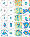 |
Fig. B.1. continued. |
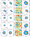 |
Fig. B.1. continued. |
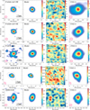 |
Fig. B.1. continued. |
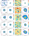 |
Fig. B.1. continued. |
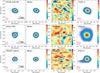 |
Fig. B.1. continued. |
Appendix C: CO(2–1) emission models
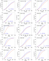 |
Fig. C.1. continued. |
Appendix D: SED models
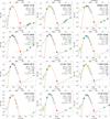 |
Fig. D.1. Same as Fig. 6. The IR observations are color coded as follows: Spitzer/IRS synthetic photometry at 34 μm (green circle); Spitzer/MIPS (yellow circles); IRAS (purple diamonds); Herschel/PACS (blue squares); ISO/ISOPHOT (blue circles); and Herschel/SPIRE (green triangles). |
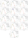 |
Fig. D.1. continued. |
All Tables
All Figures
|
Fig. 1. ALMA continuum observation (first panel), best-fit model (second panel), residual emission after subtracting the continuum model (third panel), and the integrated CO(2–1) emission (moment 0) from Lamperti et al., in prep. (fourth panel) for 00188−0856 as an example. The two contour levels in the first panel indicate the 3σ and the 0.5×peak emission levels. In the second panel, the individual components of the best-fit model are presented as a black circle (point source model) and as a dashed ellipse (deconvolved Gaussian model). The black crosses in the first, third, and fourth panels mark the fit location of the continuum peak. The red hatched ellipses represent the beam FWHM. The units are μJy beam−1 for the continuum panels and Jy km s−1 beam−1 for the CO(2–1) panel. The continuum model fits for the whole sample are shown in Fig. B.1. |
| In the text | |
|
Fig. 2. Distribution of the ∼220 GHz continuum half-light radius (rcont; see Table 3). Upper limits are indicated with arrows. The red (black) histogram bars and arrows correspond to galaxies classified as AGN (non-AGN) from optical spectroscopy. The sizes of the systems whose ALMA flux might have high (>40%) nonthermal synchrotron contributions are marked in blue (see Sect. 5.1.2). |
| In the text | |
|
Fig. 3. Comparison between the 400 pc resolution 247 GHz continuum image analyzed in Sect. 4.1 (left panel) and the higher resolution (120 pc) data (right panel) available for 17208−0014. The black cross is the position of the center measured on the 400 pc image. The contours are as in Fig. 1. The hatched red ellipses correspond to the beam FWHM of each image. The color scales are in mJy beam−1. |
| In the text | |
|
Fig. 4. Growth curve of the CO(2–1) moment 0 map for 00188−0856 as an example. The circles correspond to the observed flux within a circular aperture of radius r. The red line is the best fit model (Sect. 4.3). The deconvolved best fit profile is shown in blue and its effective radius, rCO = FWHM/2, is indicated by the vertical blue dotted line. The dashsed green line marks the ∼220 GHz continuum radius, rcont for comparison. The CO(2–1) model fits for the whole sample are shown in Fig. C.1. |
| In the text | |
|
Fig. 5. Half light radius of the 220 GHz continuum rcont vs. 0.5 × FWHM of the CO(2–1) emission rCO. Red (black) symbols mark systems classified as AGN (non-AGN) based on optical spectroscopy. Filled symbols correspond to nuclei in interacting systems and empty symbols to nuclei in mergers (see Table 1). Blue encircled symbols are galaxies with excess nonthermal emission whose continuum size estimates might be inaccurate (Sect. 5.1.2). The green line is best linear fit excluding the nuclei with rcont upper limits. The dotted line indicates the 1:1 relation. |
| In the text | |
|
Fig. 6. SED fit for 00188−0856 as an example. The data points correspond to the radio (green diamonds), ALMA ∼220 GHz from this paper (red circle), and IR (remaining points) observations. The solid green line is the 5–38 μm Spitzer/IRS spectrum. The IR observations are color coded as follows: Spitzer/IRS synthetic photometry at 34 μm (green circle); Spitzer/MIPS (yellow circles); and Herschel/SPIRE (green triangles). The solid red line is the best gray-body fit and the dashed blue line represents the best power-law fit to the nonthermal radio emission. Only the encircled symbols have been used for the fits (i.e., the ALMA point is excluded from the SED fit). The dot-dashed green line represents the expected maximum free–free emission assuming that all the LIR is produced by SF (see Sect. 4.4). The SED fits for the whole sample are shown in Fig. D.1. |
| In the text | |
|
Fig. 7. Cold molecular gas surface density (ΣH2) vs. IR luminosity surface density (ΣLIR). Galaxy symbols are as in Fig. 5. The dotted black lines indicate the maximum luminosity from an instantaneous starburst using 100% (ϵ = 1) or 20% (ϵ = 0.2) of the available cold molecular gas (see Sect. 5.2.1). The orange solid line is the Eddington luminosity limit. For points above this line, the radiation pressure is stronger than gravity (Sect. 5.5). The dashed blue lines indicate the 1 and 10 Myr depletion times for reference assuming that the IR luminosity is produced by SF. The column density (NH) axis is calculated from ΣH2 assuming a uniform mass distribution (i.e., NH = 2 × ΣH2/m(H2) where m(H2) is the H2 molecular weight). |
| In the text | |
|
Fig. 8. Logarithm of the excess mid-IR emission vs. size of the 220 GHz continuum (left panel) and size of the CO(2–1) emission (right panel). Galaxy symbols are as in Fig. 5. The solid orange line is the best linear fit to the non-AGN (black) points. In the left panel, the red box (a) marks a region of this diagram solely occupied by optically detected AGN. The blue box (b) indicates the location of very compact ULIRG nuclei (mostly unresolved by our data) with negligible excess mid-IR emission. The green box shows the location of more extended nuclei with higher mid-IR excess. |
| In the text | |
|
Fig. 9. Same as left panel of Fig. 8, but galaxies with more than 50% AGN contribution based on mid-IR observations are indicated in red (Veilleux et al. 2009; Nardini et al. 2010). |
| In the text | |
|
Fig. 10. Distribution of the 220 GHz continuum radius rcont (left) and the CO(2–1) emission radius rCO (right) for the nuclei in interacting ULIRGs. The upper limits for the 220 GHz continuum are included in the first bin and indicated by the green shaded area. |
| In the text | |
|
Fig. 11. Relation between the 9.7 μm silicate absorption and the 220 GHz continuum (left) and the CO(2–1) (middle) sizes. Right panel: 220 GHz continuum size vs. IRAS 12 μm/25 μm color relation. Symbols as in Fig. 5. For the IRAS 12 μm/25 μm color relation (right), the best linear fit to the non-AGN objects (black symbols) is log f12/f25 = (− 1.29 ± 0.04)+(1.6 ± 0.3)×10−3 × rcont/pc. |
| In the text | |
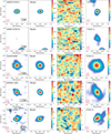 |
Fig. B.1. Same as Fig. 1. |
| In the text | |
|
Fig. B.1. continued. |
| In the text | |
|
Fig. B.1. continued. |
| In the text | |
|
Fig. B.1. continued. |
| In the text | |
|
Fig. B.1. continued. |
| In the text | |
|
Fig. B.1. continued. |
| In the text | |
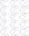 |
Fig. C.1. Same as Fig. 4. |
| In the text | |
|
Fig. C.1. continued. |
| In the text | |
|
Fig. D.1. Same as Fig. 6. The IR observations are color coded as follows: Spitzer/IRS synthetic photometry at 34 μm (green circle); Spitzer/MIPS (yellow circles); IRAS (purple diamonds); Herschel/PACS (blue squares); ISO/ISOPHOT (blue circles); and Herschel/SPIRE (green triangles). |
| In the text | |
|
Fig. D.1. continued. |
| In the text | |
Current usage metrics show cumulative count of Article Views (full-text article views including HTML views, PDF and ePub downloads, according to the available data) and Abstracts Views on Vision4Press platform.
Data correspond to usage on the plateform after 2015. The current usage metrics is available 48-96 hours after online publication and is updated daily on week days.
Initial download of the metrics may take a while.