| Issue |
A&A
Volume 650, June 2021
|
|
|---|---|---|
| Article Number | A157 | |
| Number of page(s) | 37 | |
| Section | Stellar structure and evolution | |
| DOI | https://doi.org/10.1051/0004-6361/202140361 | |
| Published online | 24 June 2021 | |
Dispersal timescale of protoplanetary disks in the low-metallicity young cluster Dolidze 25⋆
1
INAF – Osservatorio Astronomico di Palermo, Piazza del Parlamento 1, 90134 Palermo, Italy
e-mail: This email address is being protected from spambots. You need JavaScript enabled to view it.
2
INAF–Osservatorio Astrofisico di Catania, Via Santa Sofia 78, 95123 Catania, Italy
3
Smithsonian Astrophysical Observatory, 60 Garden Street, Cambridge, MA 02138, USA
4
LESIA, Paris Observatory, France
5
Astrophysics Group, Keele University, Keele ST5 5BG, UK
Received:
15
January
2021
Accepted:
7
April
2021
Abstract
Context. The dispersal of protoplanetary disks sets the timescale that is available for planets to assemble, and thus it is one of the fundamental parameters in theories of planetary formation. Disk dispersal is determined by several properties of the central star, the disk itself, and the surrounding environment. In particular, the metallicity of disks may affect their evolution, but controversial results have been published so far: disks in low-metallicity clusters appear to disperse rapidly, while some evidence supports the existence of accreting disks that are several million years old in the Magellanic Clouds.
Aims. We study the dispersal timescale of disks in Dolidze 25, the young cluster in the proximity of the Sun with the lowest metallicity, to understand whether disk evolution is affected by the low metallicity of the cluster.
Methods. We analyzed Chandra ACIS-I observations of the cluster and combined the resulting source catalog with existing optical and infrared catalogs of the region. We selected the disk-bearing population in a circular region with a diameter of 1° centered on Dolidze 25 from criteria based on infrared colors, and we selected the disk-less population within a smaller central region from the X-ray sources with O infrared counterparts. In both cases, criteria were applied to discard contaminating sources in the foreground or background. We derived stellar parameters from isochrones that were fit to color-magnitude diagrams.
Results. We derived a disk fraction of ∼34% and a median age of the cluster of 1.2 Myr. To minimize the effect of incompleteness and spatial inhomogeneity in the list of members, we restricted this calculation to stars in a magnitude range within which our selection of cluster members is fairly complete. We also adopted different cuts in stellar masses. When we compare this estimate with existing estimates of the disk fraction of clusters younger than 10 Myr, the disk fraction of Dolidze 25 appears to be lower than what is expected based on its age alone.
Conclusions. Even though our results are not conclusive given the intrinsic uncertainty on stellar ages estimated from isochrone fitting to color-magnitude diagrams, we suggest that disk evolution in Dolidze 25 may be affected by the environment. Given the poor O-star population and low stellar density of the cluster, it is more likely that the disk dispersal timescale is dictated more by the low metallicity of the cluster than by external photoevaporation or dynamical encounters.
Key words: techniques: photometric / protoplanetary disks / stars: formation / stars: pre-main sequence / X-rays: stars / open clusters and associations: individual: Dolidze 25
Candidate members and X-ray sources catalogues are only available at the CDS via anonymous ftp to cdsarc.u-strasbg.fr (130.79.128.5) or via http://cdsarc.u-strasbg.fr/viz-bin/cat/J/A+A/650/A157
© ESO 2021
1. Introduction
The dispersal of protoplanetary disks is a crucial topic in astronomy for its importance in setting the time that is available for the formation of planetary systems around young stars (e.g., Helled et al. 2014). The timescale for disk dispersal has been observationally set by determining the fraction of stars in clusters at different ages that still host a protoplanetary disk (Haisch et al. 2001; Hernández et al. 2007; Richert et al. 2018). It has been found that most of the disks disperse in a few million years (Myr): Starting from disk fractions as high as 60%–80% in very young clusters, the typical fraction in 5 Myr old clusters is about 20%. In ≥10 Myr old regions, such as the TW Hydra, σOri, and NGC 7160 associations, primordial disks become exceedingly rare, as attested by the very low incidence of less than 5% (Sicilia-Aguilar et al. 2006a; Hernández et al. 2007). However, these numbers must be interpreted as a general trend because individual stars may retain their disks for longer times (e.g., Armitage et al. 2003).
The trend outlined before refers to disks whose evolution is not affected by the surrounding environment. In the past decades, several environmental feedback mechanisms that might affect the dispersal of protoplanetary disks have been explored.
Local stellar density is important because during the dynamical evolution of the parental cluster, stars can experience close encounters with other members during which the mutual gravitational interaction may affect the evolution of their disks. During these encounters, part of the disk material can be dispersed in the surrounding medium or may even be captured by the other star (Clarke & Pringle 1993; Pfalzner et al. 2005; Thies et al. 2010). The importance of close encounters is studied by simulating the dynamical relaxation of clusters with different stellar densities with the aim of estimating the rate of destructive encounters in a time interval comparable to the disk lifetimes. For instance, Clarke & Pringle (1993) found that a density of about 100 stars/pc3 is required for a 1% likelihood of potentially destructive close encounters for 100 AU disks in 1 Myr. Steinhausen & Pfalzner (2014) found that only a negligible fraction of protoplanetary disks experiences destructive close encounters in 2 Myr in clusters with a stellar density lower than 3000 stars/pc3. Vincke et al. (2015) found that in clusters with a stellar density smaller than 90 stars/pc3, no disks shrink to 10 AU by close encounters within 5 Myr, while about 10%–17% can be dispersed down to 100 AU.
The typical stellar density of known clusters in the Milky Way shows that only the most extreme clusters such as the Arches cluster may have a stellar density so high as to result in a significant probability for destructive encounters (Olczak et al. 2012). However, a more destructive feedback would be provided by externally induced photoevaporation even in these cases. The disks are then dispersed because of the incidence of energetic UV radiation (e.g., Johnstone et al. 1998) that is emitted by nearby massive stars. UV photons dissociate and ionize hydrogen molecules and atoms, which increases the gas temperature to more than one thousand degrees and drives a photoevaporative wind away from the disk. Because the UV radiation is provided by massive stars, externally induced photoevaporation is expected to be important in clusters with at least a few thousand members that are expected to host massive stars (Weidner et al. 2010), and the effects of photoevaporation are more dramatic within a few parsecs from such massive stars. Direct observations of evaporating disks were obtained in the Trapezium in Orion (O’dell & Wen 1994; Bally et al. 2000; Fang et al. 2016), Cygnus OB2 (Wright et al. 2012; Guarcello et al. 2014), NGC 2244 (Balog et al. 2006), NGC 1977 (Kim et al. 2016), and Carina (Mesa-Delgado et al. 2016). Indirect evidence supporting a fast erosion of protoplanetary disks in the proximity of massive stars was obtained by observing a decline of the disk fraction close to massive stars or in regions with high local UV fields in massive clusters and associations such as NGC 2244 (Balog et al. 2007), NGC 6611 (Guarcello et al. 2007, 2009, 2010a), and Pismis 24 (Fang et al. 2012). Richert et al. (2015) instead found no evidence supporting a lower disk fraction near massive stars in the sample of massive clusters included in the Massive Young Star-forming complex Study in the infrared and X-ray (MYStIX) project (Feigelson et al. 2013), suggesting that evidence supporting the external disks photoevaporation found by earlier studies was affected by selection effects. This has been refuted by careful later studies of NGC 6231 (Damiani et al. 2016), Cygnus OB2 (Guarcello et al. 2016), and Trumpler 14 and 16 (Reiter & Parker 2019), for instance.
The metallicity of disks, which is typically assumed to be equal to that of their parental clusters, is also expected to play an important role in determining disk dispersion timescales by affecting the relative content of dusts, which regulates important disks properties such as opacity. The first and so far only observational confirmation of a fast erosion of disks selected from infrared photometry in low-metallicity environments has been provided by Yasui et al. (2009, 2010, 2016a) and Yasui et al. (2016b), who derived the disk fractions in six clusters in the outer Galaxy, characterized by [O/H] ∼ −0.7 dex and a dust-to-gas ratio of ∼0.001. The clusters of their sample younger than 1 Myr (Cloud2-N and -S, Sh2-209, and Sh2-208) have a disk fraction between 7 ± 1% and 27 ± 7%, which is far lower than the typical disk fraction of 60%–80% that is observed in clusters with similar ages but solar metallicity. Similarly, the only cluster in their sample with an age of 2–3 Myr (Sh2-207) has a disk fraction of 5.1 ± 4.6%, while clusters with this age and solar metallicity have a disk fraction of 30%–40%.
Yasui et al. (2010) stated that a faster dispersal of protoplanetary disks in low-metallicity environments is unlikely to be a consequence of a more efficient dust aggregation process, which instead is expected to proceed slowly because of the low dust content. Alternatively, the authors considered it more likely that the ionization fraction in low-metallicity disks is larger than in disks with higher metallicity, which increases their accretion rates. This hypothesis was supported by previous works (e.g., Hartmann et al. 2006; Hartmann 2009) claiming that accretion is mainly driven by magnetorotational instability (MRI; Balbus & Hawley 1991), whose efficiency increases with increasing disk ionization rate. Gorti & Hollenbach (2009) also claimed that far-UV (FUV) photons penetrate disks with a low dust-to-gas ratio more deeply, and that the dispersal time of disks decreases with increasing dust opacity. The general consensus has in past years shifted toward a more important role of the magnetically driven disk wind in removing mass and angular momentum from the disk, which also drives mass accretion toward the inner disk (Suzuki et al. 2010; Bai & Stone 2013; Simon et al. 2013). Because in this picture MRI is still responsible for triggering the magnetohydrodynamic (MHD) turbulence that drives the vertical gas outflow (Suzuki et al. 2010) and both mass accretion and mass-loss rate are expected to increase with increasing penetration depth of ionizing photons (Bai et al. 2016), the low disk opacity in low metallicity can still be responsible for a faster disk dispersal than at solar metallicity.
Some studies explored the possibility that low metallicity increases the effectiveness of photoevaporation in removing gas and small dust grains from protoplanetary disks. This is in line with the results obtained by Gorti & Hollenbach (2009). Focussing on photoevaporation induced by X-ray photons emitted by the central stars (Ercolano et al. 2008, 2009), Ercolano & Clarke (2010) have found that the disk dispersal timescale due to photoevaporation (tphot) increases with the disk metallicity following the relation tphot ∝ Z0.52. Following these authors, the higher efficiency of photoevaporation in low-metallicity disks is due to lower dust opacity. It is interesting to note that according to Ercolano & Clarke (2010), disk dissipation timescales are instead expected to strongly decrease with increasing disks metallicity when disks are mainly dispersed by planet formation because the higher metallicity results in a more efficient solid coagulation into planetesimals (Pollack et al. 1996; Hubickyj et al. 2005). This is in line with evidence that showed that the incidence of Jovian planets around dwarf stars increases with the metallicity of the stars (e.g., Fischer & Valenti 2005). The higher efficiency of photoevaporation in low metallicity has more recently also been confirmed by the simulations presented by Nakatani et al. (2018a, b). On the other hand, these models did not include the effects of metallicity over the stellar UV and X-ray emission. For instance, coronal X-ray radiation is dominated by line emission from highly ionized atomic species, and thus it depends on the abundance of heavy elements (Pizzolato et al. 2001).
In the context of disk evolution in low-metallicity environments, it is worth mentioning the evidence of more intense accretion rates found in stars with a disk in the Magellanic Clouds. Several works that focused on accretors in low-metallicity star-forming complexes of the Large Magellanic Clouds (De Marchi et al. 2010, 2017; Spezzi et al. 2012; Biazzo et al. 2019), on average with Z = 0.007 (Maeder et al. 1999), and Small Magellanic Clouds (e.g., De Marchi et al. 2011) reported higher mass accretion rates than for stars with masses similar to that of the Milky Way (e.g., Beccari et al. 2015). The higher accretion rates and longer accretion timescales in low-metallicity star-forming regions have been interpreted by the authors as a consequence of a less intense radiation pressure experienced by the inner disks when the dust content is smaller. These results can also be understood if the disk photoevaporation discussed above is overwhelmed by other effects that can result in longer disk lifetimes and higher accretion rates: Higher ionization, which induces far higher mass accretion rates, and a lower disk opacity, which results in a lower disk temperature, lower viscosity, and thus longer viscous timescale (Durisen et al. 2007), or a slower formation of protoplanets because the concentration of solid bodies is lower and thus the grain aggregation process is less efficient. All this slows the dispersal of protoplanetary disks down (Dullemond & Dominik 2005).
2. Dolidze 25
The young open cluster Dolidze 25 (also known as C 0642+0.03 or OCL-537; l = 212°, b = −1.3°) is one of the best targets in which to study the evolution and dispersal timescale of protoplanetary disks in a low-metallicity environment. It is one of the known rare cases of Galactic low-metallicity environments. The cluster metallicity was determined for the first time by Lennon et al. (1990) on the basis of high-resolution spectroscopy of three OB stars that were found to be deficient in metals by a factor of ∼6. This was later confirmed by Fitzsimmons et al. (1992) and Negueruela et al. (2015). The latter authors derived a metallicity −0.3 dex below solar for silicon and of −0.5 dex below solar for oxygen. Even through these values are not as low as those reported by Lennon et al. (1990) and are not fully inconsistent with the radial slope of the metallicity gradient in our Galaxy, Dolidze 25 is confirmed as one of the young clusters with the lowest metallicity known in our Galaxy when the observed data-point dispersions is taken into account (Rolleston et al. 2000; Esteban et al. 2013).
The determination of the main parameters of Dolidze 25, such as distance and age, is quite controversial. The first estimates were based on the few massive stars (about ten OB stars). Moffat & Vogt (1975) determined a distance of 5.25 kpc from UBVHα photometry. Lennon et al. (1990) placed the cluster at 3.6 kpc from an isochrone fit to the upper main sequence of the cluster. Turbide & Moffat (1993) determined an age of ∼6 Myr and a distance of ∼5 kpc from optical photometry. More recently, Delgado et al. (2010) analyzed UBVRIJHK photometry of the central area of Dolidze 25 and identified 214 candidate cluster members. They set the cluster distance equal to 3.6 kpc. These authors claimed that two distinct populations belong to the cluster: A younger pre-main-sequence population that is 5 Myr old, and an older population with an age of 40 Myr. Following studies found no evidence for such an old cluster population. For instance, Negueruela et al. (2015) set an upper limit to the cluster age of ∼3 Myr by noting that none of the most massive stars of Dolidze 25 (the O6 V star S33 and the O7 V stars S15 and S17, following the nomenclature on the WEBDA1 database) show evidence of any evolution off the main sequence, and adopted a distance of 4.5 kpc from the trigonometric parallax distance of the HII region IRAS 06501+0143 in the proximity of the cluster. Cusano et al. (2011) analyzed data of Dolidze 25 that were obtained with VIMOS at the VLT, 2MASS, and Spitzer. They set a distance of 4 kpc from the spectroscopic parallax of three OB members and an average age of 2 Myr. They also found evidence for a significant age spread and a sequential star formation process throughout the whole area. Kalari & Vink (2015) estimated an age between 2 and 3 Myr for cluster members in the center of Dolidze 25 selected from infrared photometry and the analysis of the Hα line, and found no evidence of a higher accretion in members with a disk with respect to the coeval populations with solar metallicity. In this paper, we adopt a distance to Dolidze 25 equal to 4.5 ± 0.5 kpc, estimated from the Gaia EDR3 counterparts of the 10 OB stars included in the Negueruela et al. (2015) catalog and with an error on the parallaxes smaller than 0.2 mas.
Dolidze 25 is part of a vast star-forming complex called Sh2-284 by Sharpless (1959). The most comprehensive determination to date of the pre-main-sequence population of the entire area was performed by Puga et al. (2009) based on the analysis of Spitzer observations. They selected a total of 155 class I and 183 class II objects that were clustered in different regions of the complex: In the central cluster Dolidze 25; around the large HII cavity surrounding the central cluster, which is ionized by the stars S33, S15, and S17; and in the compact HII regions IRAS 06439−0000, IRAS 06446+0029, and IRAS 06454+0020. The pillars and globules containing young stars that point toward the central cluster apparently support the hypothesis of some level of triggered star formation across the area (Cusano et al. 2011). Figure 1 shows the WISE (Wright et al. 2010) image at 12 μm of the area surrounding Dolidze 25. We mark the large area within which we searched for stars with a disk, the field observed with Chandra ACIS-I, and the regions identified and analyzed by Puga et al. (2009). In this paper we adopt the nomenclature defined by Puga and collaborators to indicate these regions.
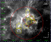 |
Fig. 1. WISE 12 μm image of the area surrounding Dolidze 25. The red circle marks the area within which we selected stars with a disk, the red box delimits the ACIS-I FoV, the dashed yellow boxes encompass the regions identified and studied by Puga et al. (2009), and the segment in the upper right corner shows the angular extent corresponding to 10 pc at the distance of Dolidze 25. |
3. Multiwavelength catalog
In this section we describe the multiwavelength catalog of the studied area. This catalog includes archival optical and infrared data. We also describe an X-ray catalog that was built from specific observations performed with Chandra ACIS-I.
3.1. Chandra ACIS-I observations
Dolidze 25 was observed with Chandra ACIS-I on 2013 December 1 and 3 (Obs.IDs: 14565 and 16543, respectively; P.I.: Guarcello). The two observations were copointed at RA = 06:45:05.10 and Dec = +00:16:15.60, with exposure times of 76.67 and 68.44 ks and both with a roll angle of 53°. We produced the Level 2 event files from the Level 1 files using the CIAO (Fruscione et al. 2006) script chandra_repro. We then combined the two event files using the tool merge_obs. Before merging the two event files, we registered the astrometry of the Obs.ID 16543 onto the 14565 through the following procedure: we first ran Wavdetect (Freeman et al. 2002) to detect sources in the two images separately, considering only the 100 brightest detected sources; we then matched the two resulting catalogs with a closest-neighbor approach; and we finally updated the astrometry of the event files using the CIAO tool WCS_update. Exposures maps in three bands (broad: 0.5–7 keV; soft: 0.5–1.2 keV; hard: 2–7 keV) were calculated using the standard CIAO tools asphist, mkinstmap, and mkexpmap.
Source detection in the three energy bands was performed using the Wavdetect and the PWDetect (Damiani et al. 1997) detection algorithms. Wavdetect detected a total of 696 sources in the broad energy band (272 in the soft band, and 420 in the hard band) adopting a threshold of 10−4, while PWDetect detected 367 sources in the broad band (657 in the soft band, 191 in the hard band) adopting a threshold of σ = 4.6. The resulting six catalogs were merged in a unique list containing 2105 candidate sources adopting a closest-neighbors approach and visually inspecting the photon distributions in the event files. Although this list was clearly dominated by spurious detections, mainly in the soft band, we decided to temporarily keep it because we validated each candidate X-ray source with a rigorous approach.
Photon extraction and source validation were performed using the IDL software ACIS Extract2 (AE, Broos et al. 2010). AE performs photon extraction by defining the point spread function (PSF) at 1.5 keV for each source, reducing the PSF size of crowded sources to 40%. The individual background regions are defined as an annulus centered on each source, with an inner radius equal to 1.1 times the 99% of the PSF, and the outer radius set in order to encompass 100 background photons. For sources in crowded regions, AE constructs a background model that accounts for the contamination due to nearby bright sources. In this latter case, the background model is improved after multiple iterations and extractions.
The AE estimates the probability for each source of being a background fluctuation, and it saves it in the parameter prob_no_source (PB). Following most of the existing works on similar data analysis (e.g., Wright et al. 2014), we considered sources as probable spurious sources when they met PB > 0.01. We thus pruned our list by removing all isolated sources with PB > 0.01. If a group of crowded sources met the requirement PB > 0.01, we removed only the faintest source and then we repeated the photon extraction process for the remaining sources in the attempt of improving their PB. After repeating the procedure five times and after a visual inspection of the sources marked by AE as probable spurious detections due to the hook-shaped feature discovered in the Chandra PSF3, we removed 1487 sources from the initial list, producing a final list of 618 confirmed sources. Figure 2 shows an RGB Chandra ACIS-I image of the combined event files and the positions of the validated X-ray sources, together with the contours of the diffuse emission at 8 μm from Spitzer-IRAC observations.
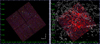 |
Fig. 2. Combined Chandra ACIS-I Images of Dolidze 25. In the left panel, we show an RBG image, with events in the hard energy band marked in red, those in the medium band (1.21–1.99 keV) are plotted in green, and those in the soft band are shown in blue. In the right panel, the white polygons mark the contours of the continuum emission at 8 μm from Spitzer-IRAC, while the red circles mark the position of the validated X-ray sources. |
In each of the five iterations of the photons extraction process, we allowed AE to correct the source positions. Following the AE guidelines, three position estimates were calculated for each source: the mean data position, which is obtained from the centroid of the extracted events and is typically used for on-axis sources (θ < 5′); the correlation position, which is calculated from the correlation between the PSF and the events distribution and is typically used for off-axis sources (θ > 5′); and the maximum likelihood position, which is calculated from the maximum likelihood image of source neighborhood and is typically used for crowded sources. The catalog of the X-ray sources, which is made available at the CDS, is described in Appendix A.
3.2. Optical and infrared catalogs
We collected the optical and infrared data available in a circular area with a radius of 0.5° (39.3 pc at the distance of 4500 pc) centered on Dolidze 25 in order to cover not only the cluster, but also a significant part of the surrounding parental cloud. Table 1 shows the list of the catalogs we used. Some of these catalogs were not directly necessary for the aim of this paper, but they were included nevertheless for future analysis of the stellar population of Dolidze 25 and Sh2-284. In Table 1 we show the total number of sources in the selected region for each catalog, together with the number of sources we retained after pruning spurious sources, artifacts, and sources with unreliable photometry following the various explanatory manuals or the references listed in the last column. The criteria adopted to clean each catalog are summarized in the criteria column.
Optical and infrared catalogs.
The optical photometry is provided by the Second Data Release of the VST Photometric Hα Survey of the Southern Galactic Plane and Bulge (VPHAS+, Drew et al. 2014), the Second Data Release of the INT WFC Photometric Hα Survey of the Northern Galactic Plane (IPHAS, Barentsen et al. 2014), the Panoramic Survey Telescope and Rapid Response System (Pan-STARRS, Chambers et al. 2016), the Second and Early Third Data Release of the Gaia catalog (Gaia Collaboration 2016), which provides parallaxes for 31 531 sources and radial velocities for 205 sources, and the optical catalog published by Delgado et al. (2010) that is based on observations taken with ALFOSC at the 2.6 m Nordic Optical Telescope (NOT), which only covers a small 7′×8′ central area. Infrared photometry is provided by the Two Micron All-Sky Survey (2MASS) Point Source Catalog (Cutri et al. 2003) and the tenth data release of the UKIRT InfraRed Deep Sky Surveys (UKIDSS, Lawrence et al. 2007) in the JHK bands, together with the catalog obtained from observations with Spitzer-IRAC during the Cycle 4 (2005 March 28, Program ID: 3340, P.I.: Neiner), presented in Puga et al. (2009), and the AllWISE Source Catalog (Wright et al. 2010). We also included 2090 optical light curves obtained from the Convection, Rotation and Planetary Transits satellite (CoRoT, Baglin et al. 2006) taken with a cadence of 32 s or 512 s; and the spectral classification of 145 stars obtained from the Fourth Data Release of the Large sky Area Multi-Object Spectroscopic Telescope (LAMOST) based on observations of the 4 m telescope located at the Xinglong Observatory northeast of Beijing (China, Luo et al. 2015). Figure 3 shows the spatial coverage of the catalogs included in the multiband catalog. Most of them have a rather uniform distribution, with a clear overdensity of sources in the center of the field that roughly corresponds to the cavity cleared by Dolidze 25. Another overdensity is detected westward of the central cavity. The distribution of the UKIDSS sources is easily explained by the fact that the adopted pruning criteria removed most of the sources at the CCD edges.
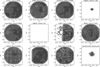 |
Fig. 3. Spatial coverage of the sources with good photometry in the catalogs. A central overdensity, corresponding to the approximate location of Dolidze 25, is evident in all the catalogs. |
3.3. Merged catalog
The optical, infrared, and X-ray catalogs were merged into a multiwavelength catalog with the procedure described in detail in Appendix B. The catalog contains 101 722 entries. In particular, 463 of the 618 X-ray sources matched at least one optical-infrared (OIR) counterpart. Considering the multiple coincidences between X-ray, optical, and infrared sources, the catalog contains a total of 593 X+OIR sources, with an expected contamination by spurious coincidences of about 10%.
4. Selection of stars with a disk
Stars with a disk were selected by adopting criteria based on 2MASS, UKIDSS, IRAC, and WISE photometry. However, these methods potentially also select various types of contaminants, for instance, extragalactic sources, giants with circumstellar dust, PAH-contaminated sources, and foreground stars. In order to obtain an inclusive selection of stars with a disk from which all possible contaminants were removed, we first selected all stars that met at least one of the criteria defined to select stars with a disk, and then we pruned the list by applying different tests, each aimed at selecting specific classes of contaminants (see Fig. 4).
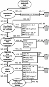 |
Fig. 4. Summary flowchart of the procedure adopted to select stars with a disk and pruned candidate contaminants from the list. In each step represented by an oval, the list is pruned of a given class of contaminants. For any selection of contaminants, sources are verified with the corresponding test shown in the boxes. A detailed description of the tests is provided in the text. |
4.1. Initial list of candidate stars with a disk
The preliminary list of candidate stars with a disk was produced by selecting all sources satisfying at least one of the criteria defined by Gutermuth et al. (2009), Guarcello et al. (2013), Koenig & Leisawitz (2014):
-
from the IRAC [3.6]–[4.5] vs. [4.5]–[5.8] diagram, sources with [3.6]–[4.5] > 0.7 AND [4.5]–[5.8] > 0.7;
-
from the IRAC [3.6]–[5.8] vs. [4.5]–[8.0] diagram, sources with [4.5]−[8.0]> 0.5 AND [3.6]−[5.8]> 0.35 AND [3.6]−[4.5]≤0.5 + 0.14 × ([4.5]−[8.0]−0.5);
-
from the IRAC [3.6]–[4.5] vs. [5.8]–[8.0] diagram, sources with [3.6]–[4.5] > 0.2 AND [5.8]–[8.0] > 0.3;
-
from the IRAC [4.5]–[5.8] vs. [5.8]–[8.0] diagram, sources with −0.1 ≤ [4.5]–[5.8] < 1.4 AND [5.8]–[8.0] > 0.2;
-
from the WISE [3.4]–[4.6] vs. [4.6]–[12] diagram, sources with 2 ≤ [4.6]–[12] < 4.5 AND [3.4]−[4.6]> 2.2 − 0.42 × ([4.6]–[12]) AND [3.4]−[4.6]> 0.46 × ([4.6]–[12]) − 0.9;
-
from the WISE [3.4]−[4.6] vs. [4.6]–[12] diagram, sources with [3.4]−[4.6]> 0.25 AND [3.4]−[4.6] < 0.9 × ([4.6]–[12]) − 0.25 AND [3.4]−[4.6]> − 1.5 × ([4.6]–[12]) + 2.1 AND [3.4]−[4.6]> 0.46 × ([4.6]–[12]) − 0.9 AND [4.6]–[12] < 4.5;
-
from the J − H vs. [3.4]–[4.6] diagram, sources with H − K > 0 AND H − K > −1.76 × ([3.4]−[4.6]) + 0.9 AND H − K < (0.55/0.16) × ([3.4]−[4.6]) − 0.85 AND [3.4] ≤ 13.
These criteria were applied only to sources whose errors in the relevant magnitudes were smaller than 0.1m and colors lower than 0.15m. The loci defined by these criteria are shown in Fig. 5 and in Figs. D.1 and D.4. The resulting preliminary list of candidate stars with a disk contains 862 sources. This list was then pruned by removing different classes of contaminants, as explained below.
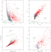 |
Fig. 5. Subset of the infrared and optical-infrared diagrams of all sources in the studied field that meet the criteria of good photometry (e.g., error in magnitude smaller than 0.1m and in color smaller than 0.15m). The dashed lines show the isochrones for ages 0.5 Myr, 1.5 Myr, 3 Myr, 5 Myr, 8 Myr, and 10 Myr, and with metallicity Z = 0.004 (Delgado et al. 2010) from the PARSEC models, plotted adopting a distance of 4.5 kpc and AV = 2.7m. Red dots mark the selected stars with a disk that we retained in the final list. We also show the loci defined to select stars with a disk and contaminants, delimited by red and green lines. In particular, we show the loci expected to be populated by giants, stars with unreliable excesses, foreground stars, and YSOs with a disk in these diagrams. All diagrams are shown in Appendix D. |
4.2. Candidate giants with circumstellar dust
Evolved giants with circumstellar dust can have intrinsic infrared colors that can mimic the spectral energy distribution (SED) that is typical of stars with a disk. In order to account for this contamination, we used the PARSEC isochrones4 (Bressan et al. 2012) in order to define the expected loci in some color–magnitude diagrams in which giants with circumstellar dust and zero extinction can be found. We then projected these loci along the specific extinction vectors. We defined these loci after testing different compositions of the circumstellar dust using the available options on the PARSEC web interface. After inspecting all the possible criteria, we used those resulting in independent selections. We list them below.
– Stars in the r vs. r − i Pan-STARRS diagram brighter than the line drawn by projecting the point [-0.1,11] along the extinction vector.
– Stars in the J vs. J − K diagram brighter than the line drawn by projecting the point [0,11] along the extinction vector.
– Stars in the [4.5] vs. [4.5]–[8.0] diagram with [4.5]−[8.0] < 0.
– Stars in the [3.4] vs. [3.4]–[4.6] diagram brighter than the line [3.4] = 1.56 × ([3.4]−[4.6]) + 9.31.
– Stars in the [3.4]–[4.6] vs. [12]–[22] diagram with
[12]−[22] < 1.9 AND
[3.4]−[4.6] < ([12]−[22]) − 0.45
(criterion defined by Koenig & Leisawitz 2014).
– SED analysis (see below).
These loci are shown in the Figs. 5, D.1, D.2, and D.4. For each star, the tests were considered positive, that is, suggesting that the star is a contaminant, when the star was located in the defined locus of giant stars. The SED test was applied to the candidate stars with a disk that met at least one of the other criteria adopted to select candidate giants. In this test, we used the Python SED fitter tool sedfitter5 developed by Robitaille (2017). The tool allowed us to fit the observed SEDs with synthetic SEDs produced from an extensive set of models of young stellar objects (YSOs) with different properties of the central star, disk, envelope, bipolar cavities, and surrounding medium. We added the WISE, Pan-STARRS, and SDSS filters to the available convolved filters using the Python codes mkfilter.py and filtermanage.py that are publicly available6. We considered this test to be positive when the observed SED did not fit that of any YSO model7.
For each candidate star with a disk selected as possible background giant, we thus counted the number Ntest of tests that we were able to perform and the number Npositive of positive tests. As shown in Fig. 4, we removed stars for which Npositive ≥ 0.5Ntest from the list of stars with a disk as candidate giants.
4.3. Candidate extragalactic sources
The infrared colors of galaxies of different types (e.g., AGN and PAH galaxies) in the IRAC and WISE bands are similar to those of stars with a disk. However, they can be distinguished from YSOs by their typical blue optical colors and faint magnitudes. We discarded candidate galaxies from the sample of stars with a disk in two steps. First, we adopted an approach similar to the one used to select giants with circumstellar dust by defining tests aimed at selecting candidate galaxies and counting the number of positive over the total number of tests for each star with a disk. These tests were defined by adopting criteria introduced by other authors (Gutermuth et al. 2009) or by plotting the extragalactic sources included in existing surveys in infrared diagrams (Stern et al. 2005; Treister et al. 2006; Rafferty et al. 2011; Koenig & Leisawitz 2014). We show this list below.
– candidate PAH galaxies from the IRAC [4.5]–[5.8] vs. [5.8]–[8.0] diagram, with the criteria
[4.5]−[5.8] < 1.05 × ([5.8]−[8.0]−1)/1.2 AND
[4.5]−[5.8] < 1.05 AND [5.8]−[8.0]> 1.
– PAH galaxies from the IRAC diagram [3.6]–[5.8] vs. [4.5]–[8.0], with the criteria
[3.6]−[5.8] < 1.5 × ([4.5]−[8.0]−1)/2 AND
[3.6]−[5.8] < 1.5 AND [4.5]−[8.0]> 1 AND
[4.5]> 11.5.
– candidate AGN from the IRAC diagram [4.5] vs. [4.5]–[8.0], with the criteria
[4.5]−[8.0]> 0.5 AND
[4.5]> 13.5 + ([4.5]−[8.0]−2.3)/0.4 AND
[4.5]> 13.5;
– candidate AGN from the IRAC diagram [4.5] vs. [4.5]–[8.0], with the criteria
[4.5]−[8.0]> 0.2 AND
([4.5]> 14.5 − ([4.5]−[8.0]−1.2)/0.3 or [4.5] > 14.5);
– candidate galaxies from the WISE diagram [3.4]–[4.6] vs. [4.6]−[12] with the criteria
[4.6]−[12]> 2.3 AND
[3.4]−[4.6]> 0.2 AND
[3.4]−[4.6] < 1.0 AND
[3.4]−[4.6] < 0.46 × ([4.6]–[12]) − 0.78 AND
[3.4] > 13.0.
These loci are shown in the Figs. D.1 and D.4. We then marked each source for which Npositive ≥ 0.5Ntest as a candidate extragalactic contaminant.
We then took advantage of the expected blue optical colors and faint magnitudes of extragalactic sources to reclassify some sources marked as possible galaxies as stars with a disk. We first used the catalogs published by Brescia et al. (2015) and Usatov (2018) to define a locus populated by extragalactic sources in the following diagrams: r vs. r − i, g vs. g − r, and r vs. g − r (both VPHAS and Pan-STARRS, see Fig. D.2). We then repeated the adopted strategy by calculating the ratio Npositive/Ntest for each source, where here a test is positive when the given star is located in these loci of extragalactic sources. We then reclassified the sources for which Npositive < 0.5Ntest as stars with a disk. This procedure should in principle also help us to avoid discarding genuine stars with a disk with blue optical colors due to accretion and/or scattering (discussed in Sect. 4.6), which are expected to be more blue in g − r than in r − i.
We also reclassified candidate extragalactic sources with a high excess in r − Hα as stars with a disk. This excess is typical of accreting stars with a disk. To select these stars, we used the IPHAS and VPHAS r − i vs. r − Hα diagrams (see Fig. D.3). In the first diagram we selected sources with r − Hα higher than the colors of the zero-age main sequence (ZAMS) locus with EWHα = −40 Å and EB − V = 1 defined by Barentsen et al. (2011), while in the second diagram we used an ad hoc lower limit for r − Hα. We also reselected candidate galaxies with [3.6] < 15.3m as stars with a disk. This limit was chosen by plotting the sources from the extragalactic catalogs compiled by Treister et al. (2006) and Rafferty et al. (2011) in the [3.6] vs. [3–6]–[4.5] diagram.
4.4. Candidate shock- or PAH-dominated sources
Another class of possible contaminants are sources whose photometry in the [5.8] and [8.0] bands is contaminated by nebular PAH emission or unresolved knots of shock emission. We followed the prescription presented in Gutermuth et al. (2009) to select candidate contaminants of these two classes, and discarded those whose SED did not fit any YSO model (3 candidate unresolved knots of shock emission, and 63 PAH-contaminated sources). The typical loci populated by PAH-contaminated sources and unresolved shocks in the [3.6]–[4.5] vs. [4.5]–[5.8] diagram are shown in Fig. D.1
4.5. Foreground stars and unreliable excesses
The YSOs that lie in the foreground of Dolidze 25 can contaminate our list of members with a disk. Even though Gaia EDR3 parallaxes cannot be used to identify low-mass stars associated with Dolidze 25 and the Sh2-284 cloud because of their large distances, they can still be useful to select and discard stars in the foreground. However, because distances obtained by simply inverting Gaia parallaxes are not fully reliable for distances larger than 1 kpc (e.g., Bailer-Jones et al. 2018), we also adopted a photometric criterion. We thus selected and removed as candidate foreground objects stars with a disk with a parallax error smaller than 0.2 mas, a distance from Gaia parallaxes smaller than 2.5 kpc, and the color i − z from Pan-STARRS lower than 0.25m.
We also defined the following criteria to select objects with unreliable excesses:
– Stars bluer than the expected pre-main sequence locus in the i vs. i − z (Fig. D.2) or J vs. J − K (Fig. 5) diagrams.
– Stars with blue colors in the i − z vs. z − y diagram (Fig. D.3).
– Stars with colors in the g − r vs. r − i (Fig. D.3) or J − H vs. H − K (Fig. 5) diagrams typical of low-extinction sources.
– Stars lying in the branch populated by low-extinction M stars in the r − i vs. i − J diagram (Fig. 5).
– Stars with [3.6]−[4.5] < 0.15 and [5.8]−[8.0] < 1.2 in the [3.6]−[4.5] vs. [5.8]–[8.0] diagram (Fig. D.4).
– Stars with [4.5]−[5.8] < − 0.3 in the [3.6]–[4.5] vs. [4.5]–[5.8] diagram (Fig. D.1).
Objects selected according to one of the above conditions were removed from the list of stars with a disk when their SEDs were compatible with photospheric models with an extinction AV between 0m and 100m, or when they were not compatible with any YSO model, or when low extinction or distance were suggested by other diagrams.
4.6. Blue stars with excesses
Candidate stars with a disk populating the expected locus of foreground main-sequence stars in optical color–magnitude diagrams are not necessarily contaminants (stars in the foreground or galaxies, which have already been removed from the list at this step, however). They can also be genuine stars with a disk that we retained in our list of disks by classifying them as blue with excesses, (BWE; Guarcello et al. 2010b) stars with a disk.
The optical colors of stars with ongoing accretion and with thick disks can be affected by the emission from accretion hot spots that are heated by the accreting material and light scattered along the line of sight by the dust in the disks. In the paradigm of magnetospheric accretion (Muzerolle et al. 1998), the accreting material funneled by the magnetic field falls onto the star at free-fall velocities of a few hundred km s−1. The energy released by the accretion shock heats the surrounding stellar atmosphere up to more than 10 000 K (accretion hot spot), emitting soft X-rays, UV, and optical radiation at short wavelengths (Calvet & Gullbring 1998). In addition, micron-size dust grains in protoplanetary disks can scatter part of the optical stellar emission along the line of sight. Because short-wavelength optical photons are more efficiently scattered than long-wavelength photons, the scattered light modifies the optical SED of stars with a disk, which causes optical colors to appear bluer than photospheric values (e.g., Guarcello et al. 2010b).
We selected the candidate stars with a disk with optical colors bluer than the expected pre-main-sequence locus in the following diagrams: r vs. r − i, and g vs. g − r, and r vs. g − r (both VPHAS and Pan-STARRS, see Fig. D.2), and discarded from our list of stars with a disk the sources that are bluer than the expected pre-main-sequence locus in the J vs. J − K diagram (e.g., they have J − K colors typical of foreground objects), or have [3.6]−[4.5] < 0.2, [5.8]−[8.0] < − 0.3, or whose SED does not fit any YSO model.
4.7. Final list of stars with a disk
After the pruning process, the list of stars with a disk contains 659 stars. Figures 5, D.1–D.4 show the color–color and color–magnitude diagrams of all stars with good photometry in the studied field, selected stars with a disk, and the loci we used to define all the adopted tests. Figure 6 shows the spatial distribution of the stars with a disk in Dolidze 25 and the surrounding Sh2-284 cloud. Compared with the selection of stars with a disk made by Puga et al. (2009), we selected about twice more objects (659 vs. 329 sources).
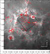 |
Fig. 6. Spitzer-IRAC image in the [8.0] band of Dolidze 25 and the surrounding Sh2-284 complex. The positions of selected stars with a disk are marked (red circles). The black square delimits the field observed with Chandra. |
5. Candidate young stars without a disk
The intense magnetic activity of pre-main-sequence stars produces a stronger X-ray emission than in older stars (Montmerle et al. 1996). Young stars in star-forming regions can thus be selected and separated from other sources in the same field of view by requiring detection in X-rays observations. As explained in Sect. 3.1, the central cavity of Sh2-284 populated by Dolidze 25 stars was observed with Chandra ACIS-I, and we detected and validated 618 X-ray sources. Of these sources, 486 match at least one optical-infrared star in our multiwavelength catalog (when the multiple coincidences are considered, our catalog contains 542 X-ray sources with OIR counterparts, see Sect. 3.3).
Although the sample of X+OIR sources is expected to be dominated by young stars in the area, it can still contain a significant number of sources that are not associated with Dolidze 25, such as magnetically active stars that are not in the pre-main-sequence phase, which must be identified and removed from the list of candidate members of the cluster. First, we considered the 131 X-ray sources that do not match any OIR source. These sources can either truly be members of Dolidze 25 with very high extinction, false-negatives produced in the catalog-merging procedure, or extragalactic sources. Figure 7 shows the distribution of the mean photon energy and the net counts in the broad energy band of all the validated X-ray sources. We separately show those of the X-ray sources with and without an OIR counterpart. The distribution of the mean photon energy of all X-ray sources and those with OIR counterparts peaks at ∼2.2 keV. The distribution of the mean photon energy of the X-ray sources without counterpart has two peaks, one peak at ∼2.5 keV and another at about 4 keV. This may suggest that this sample contains both stars and extragalactic sources. However, the typical net counts of these sources is ≤10 photons, which precludes further investigation. Because we cannot distinguish between these two possibilities, we removed the X-ray sources without OIR counterpart from the list of disk-less members. The exception to this is a group of 16 X-ray sources without OIR counterparts that has a net count of more than 50 photons and a mean photon energy between 1.2 and 3.2 keV. We retained this in our list. We will attempt to constrain their nature by analyzing their X-ray spectra in a forthcoming work.
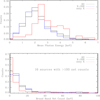 |
Fig. 7. Distribution of the mean photon energy and net counts in the broad energy band for the validated X-ray sources. We show the X-ray sources with and without OIR counterpart separately. |
Then we selected and removed the X+OIR sources that are likely in the foreground or in the background. In order to search for extragalactic contaminants among the X-ray sources with OIR counterpart, we used the IRAC and WISE color–color and color–magnitude diagrams in which we defined the typical loci of extragalactic sources (Figs. D.1 and D.4). Only 6 X+OIR sources that were not classified as disk-bearing members populate these loci. Two of these sources lie in the loci of extragalactic sources in more than half of the diagrams in which they can be plotted, and thus they were removed from the list of candidate disk-less young stars. In order to select candidate X+OIR sources in the foreground, we first removed 43 X+OIR sources with errors in the Gaia parallaxes smaller than 0.2 mas and distances from parallax smaller than 2.5 kpc. We also removed other 20 X+OIR sources with large parallax errors that lay in the foreground or BWE loci in most of the diagrams in which they can be plotted. After this pruning, we compiled a list of 379 candidate unique X-ray sources with at least one OIR counterpart. These are candidates for being disk-less young stars of Dolidze 25. As expected, the removed X+OIR sources have an almost uniform spatial distribution.
Figure 8 shows a selection of optical and infrared diagrams of all stars in the ACIS FoV that match the criteria for good photometry, the candidate stars with a disk (inside the ACIS FoV), the members without a disk, and the X+OIR sources removed from the list of disk-less stars. In the optical color–magnitude diagrams, the pre-main-sequence locus at the distance and extinction of Dolidze 25 is well defined by the selected candidate members of the cluster. Two candidate members without a disk show a significant excess in Hα although they are not included in the list of stars with a disk, and would need to be further investigated to discern their nature. The X+OIR sources discarded from the list of members clearly show colors of foreground and background sources. Figure 9 shows the spatial distribution of both disk-less and disk-bearing stars inside the cavity hosting Dolidze 25. With respect to the regions identified by Puga et al. (2009), we have identified a new group of members that is rich in disk-less stars within the cavity between the RN and Cl2 regions.
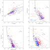 |
Fig. 8. Diagrams of all sources in the ACIS FoV that meet the criteria of good photometry (gray points). Figure layout and symbols are the same as in Fig. 5. The large dots are: candidate stars with a disk inside the ACIS FoV (red), candidate young stars without a disk (blue), and X+OIR sources in the foreground or background (yellow). |
6. Comparison with members from the literature and final selection
The list of members compiled by Delgado et al. (2010) over a small area at the center of Dolidze 25 includes 29 stars with IR excesses, 102 main-sequence stars, and 103 pre-main-sequence stars. From these stars, we retrieved in our list of members 8 of their stars with infrared excesses (3 disk-less and 5 with a disk), 9 of their main-sequence members (all as disk-less members), and 20 of their pre-main-sequence stars (17 disk-less and 3 with a disk). After verifying the positions in the various optical and infrared diagrams of the stars selected by Delgado et al. (2010) and not by us, we added only one star from their lists of members, while the other stars do not lie together with the other cluster members in all color–color and color–magnitude diagrams and thus were not included in our list of members.
Puga et al. (2009) selected 155 class I and 183 class II sources in the area around Dolidze 25 from specific Spitzer-IRAC observations of Sh2-284. Our list of disk-bearing members has 116 class I and 153 class II sources in common with their list. We discarded 17 of their members as probable contaminants. With the exception of 3 stars that we added in our list, the few stars in the Puga et al. (2009) list that are not included in our list do not meet the criteria we defined for good photometry in the IRAC bands.
Negueruela et al. (2015) studied optical spectra of the brightest stars in the field of Dolidze 25. Because the criteria that we defined to select and discard candidate giant stars with circumstellar dust (Sect. 4.2) and foreground stars (Sect. 5) are not designed for intermediate massive members of Dolidze 25, these stars were automatically discarded from our list of members. We thus analyzed the stars included in the list of Negueruela et al. (2015) separately and included 11 of these OB stars in our list of members. According to Gaia data, we confirm that stars S9 and HD 48691 (from parallaxes) and HD 48807 (from proper motion) are likely stars in the foreground. We also confirm the infrared and Hα excesses of the stars S24 and SS57, classified as Herbig Be stars by Negueruela et al. (2015). When we consider the stars with errors in parallax smaller than 0.2 mas among these stars, the median distance of these stars is 4.5 ± 0.5 kpc. As explained in Sect. 2, this is the distance value that we adopted to plot the isochrones in all the color-magnitude diagrams shown in the paper.
Cusano et al. (2011) performed a spectroscopic and photometric analysis of 23 pre-main-sequence objects in the center of Dolidze 25. Two of the 6 stars identified by Cusano et al. (2011) as disk-less members are detected in X-rays and classified as disk-less members in our work as well. Because the spectroscopic evidence supporting the membership to Dolidze 25 of the remaining 4 stars is solid, we changed their status to disk-less members. We also selected 12 of the 17 stars in the list of class II objects of Cusano et al. (2011) as stars with a disk. Of the remaining 5 stars, 3 do not match our criteria for good photometry in the diagrams we used to select stars with a disk, and two were discarded as likely background giant contaminants (an F0V and F2V star, according to the spectral classification provided by Cusano et al. 2011). We reclassified these five stars as stars with a disk of Dolidze 25. We also classified two other stars classified as class I objects by Kalari & Vink (2015) as class II objects.
Our final list of confirmed young stars associated with Dolidze 25 and Sh2-284 contains 667 stars with a disk, 424 stars without a disk, and 10 spectroscopically confirmed massive and intermediately massive stars. The final catalog of the candidate young stars in Dolidze 25 and the surrounding area, available at the CDS, is described in Appendix F.
7. Disk fraction in Dolidze 25
In this section we calculate and analyze the disk fraction of Dolidze 25, where we selected both the disk-bearing and disk-less stellar population. A simple visual inspection of Fig. 9 shows that the spatial distribution of selected members inside the ACIS FoV is not homogeneous. The candidate members are apparently separated into two main populations: the main cluster inside the cavity, and a population in the north along the bright rim of the cavity, mainly composed of cluster 2, the bright-rimmed cloud RN, and a population of disk-less sources between these two groups. An accurate analysis of the disk fraction in Dolidze 25 needs to account for any possible difference between the properties of these two populations, such as stellar age and mass content.
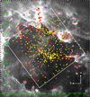 |
Fig. 9. IRAC image in the [8.0] band of the field around Dolidze 25, together with the position of candidate stars with a disk (red), without a disk (yellow) and spectroscopic members (blue). We also indicate the limits of the Chandra ACIS-I field with a square. |
7.1. Analysis of the spatial distribution of members
A detailed analysis of the subclustering in Dolidze 25, which would require high-quality astrometric and stellar dynamic data as well, is beyond the scope of this paper. However, we wish to verify whether suitable statistical tests support the existence of two separated groups of cluster members. With this aim, we calculated the minimum spanning tree (MST) of the cluster (Barrow et al. 1985). The MST consists of the unique set of branches connecting all points in a 2D scatter plot with the minimum total length and without producing closed loops. We calculated the MST of the selected members using the analyses of phyogenetics and evolution (ape) R package (Paradis & Schliep 2018).
Figure 10 shows the MST built on all the candidate members found in the ACIS FoV. In order to discern between clustered and nonclustered members, we also estimated the critical branch length as the branch length at which the cumulative distribution of the branch lengths changes slope (Gutermuth et al. 2009). This calculation resulted in a critical branch length of 34 3, corresponding to a projected distance of 0.75 ± 0.08 pc at a distance of 4.5 kpc. We then considered all members that are separated from the closest member by a distance smaller than the critical branch length as clustered, and we called the remaining stars “sparse”. In Fig. 10, clustered stars are marked with filled dots and the sparse population with empty dots. The MST confirms the presence of two main stellar groups: a group inside the cavity, corresponding to the main cluster, and an elongated northern group lying along the front of the cavity (called hereafter the central and northern populations, respectively). Several other small groups are identified, but the identification of these groups as real subclusters is beyond the scope of our work. We also applied the method introduced by Allison et al. (2009) to explore the presence of mass segregation in the cluster. We conclude that our data do not support this possibility.
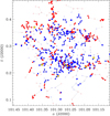 |
Fig. 10. Minimum spanning tree built on all the members selected inside the ACIS FoV. Members without a disk are marked with blue dots and those with disks with red dots. The yellow stars mark the position of the most massive members. Filled dots mark the position of clustered members, i.e., members that are closer than 34 |

7.2. Extinction across the field
To estimate a reliable disk fraction for Dolidze 25 and compare it with that of other clusters, we need to quantify individual stellar parameters. We need to estimate the median age of cluster members to compare the disk dispersal timescale in Dolidze 25 with that of other young clusters, while stellar masses are necessary to account for the incompleteness of our selection. Stellar parameters were evaluated by placing cluster members in derreddened color–color and color–magnitude diagrams after individual extinctions were evaluated. Individual extinctions can in principle be estimated by calculating the displacement along the extinction vector of stars in color–color diagrams from a representative isochrone drawn assuming zero extinction.
The reliability of the estimate of individual extinctions may depend on the particular diagram that is used. A better estimate is possible if the adopted isochrone is sufficiently regular in order to avoid unrealistic discontinuities in the distribution of the resulting extinctions, and if the slope of the isochrone is sufficiently different from that of the extinction vector in order to avoid that photometric uncertainties would result in too large extinction uncertainties.
After several tests, we adopted the Pan-STARRS diagram Qrizy vs. i − z (Fig. 11) to estimate individual stellar extinctions. Qrizy is the reddening-free color index (r − i)−(i − z) × Er − i/Ez − y (similar to those defined by Damiani et al. 2006) where the ratio Er − i/Ez − y in the Pan-STARRS bands is equal to 2.214 according to the reddening law of Cardelli et al. (1989) and O’Donnell (1994; in Appendix C we summarize the extinction coefficients adopted in all the bands used in this work). Because the optical colors of disk-bearing stars may not be fully representative of their stellar properties due to the emission from accretion hotspots, light scattered by the disk, and the partial occultation of the stars by their disks (see Sect. 4.6), we calculated individual extinction for the members with and without a disk, but we used only the estimate from the latter to derive the extinction map and median extinction of the cluster. As evident in the right panel of Fig. 11, the PARSEC isochrones in the Qrizy vs. i − z diagram, considering only the PMS stage, present an horizontal segment at about Qrizy = 0.1, which results in an unrealistic discontinuity in the distribution of the resulting extinctions. We thus averaged the i − z values of the isochrones, increasing those for points with Qrizy > 0.1 by 0.07m and decreasing those with Qrizy < 0.1 by the same amount. Moreover, we restricted the calculation of extinction from Qrizy vs. i − z only for stars with −0.15m ≤ Qrizy ≤ 0.7m, which is the range covered by the adopted isochrone.
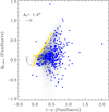 |
Fig. 11. Pan-STARRS Qrizy vs. i − z diagram of all sources in the studied field with errors in colors smaller than 0.15m. The blue dots mark the observed colors of the candidate members of Dolidze 25, and the yellow dots mark their positions after dereddening their colors. The dashed lines mark the zero-extinction low-metallicity PARSEC isochrones for the pre-main-sequence phase assuming an age of 1.5 Myr. |
We computed the individual extinctions for 241 candidate disk-less members. The 25%, 50%, and 75% quantiles of the resulting AV distribution are equal to 1.7m, 2.3m, and 3.2m, respectively. Figure 12 shows the distributions of individual extinctions of all disk-less members. We separately plot those of the stars in the central group, the northern group, and the sparse population. The right panel also shows the resulting extinction map of the entire ACIS field, plotted together with the contours marking the emission levels at 8.0 μm in IRAC images, which help to visualize the distribution of nebular dust emission. Although the highest extinction values are observed where the dust emission is higher, such as in the northern part of the field, the AV distributions of the central and northern groups are quite similar. The differences are within one magnitude.
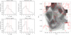 |
Fig. 12. Left: distribution of the individual extinctions of all disk-less members. We separately plot those for sources in the central cluster, northern group, and in the sparse population. The vertical lines mark the median and the 25% and 75% quantiles of each distribution. Right: extinction map in the ACIS field. The red lines mark the emission level at 8.0 μm from IRAC images. The green boxes roughly delimit the central and northern groups. |
7.3. Mass and age of cluster members
Masses and ages of candidate members were estimated by interpolating their positions in selected derreddened color–magnitude diagrams on a grid computed using the 0.5–10 Myr low-metallicity PARSEC isochrones. Details of how individual masses and ages were calculated are provided in Appendix E. Figure 13 shows the distribution of individual stellar ages calculated for the disk-less and disk-bearing candidate members (the latter only within the ACIS field). The age distribution shows a clear peak at about log(age)∼6.0 Myr, with a median age equal to log(age)median = 6.2 Myr, with a standard deviation of 0.3 Myr.
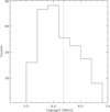 |
Fig. 13. Distribution of individual stellar ages for candidate members within the ACIS field. The vertical lines mark the median value of the distribution. The distribution peaks at about log(age)∼6.0 Myr, with a median age equal to log(age)median = 6.2 Myr. |
Our estimate of the median age of Dolidze 25 is smaller than the estimate presented by Delgado et al. (2010), who selected two populations of candidate members from optical and infrared photometry, the youngest with a median age of log(age) = 6.7 ± 0.2 Myr coexists with a population older than 40 Myr, and by Turbide & Moffat (1993), who estimated an age of 6 Myr by fitting the upper main sequence to 12 candidate bright members. These differences can be understood as a consequence of the fact that our study is the first that selects disk-less members (for which age estimation from color-magnitude diagrams is more reliable) down to the low-mass star regime. In addition, the existence of an old population suggested by Delgado et al. (2010) was not confirmed by other authors. Our estimate is instead more similar to what was found by Negueruela et al. (2015), who set an upper limit to the cluster age of 3 Myr from the photometric analysis of the most massive stars in the clusters (one O6V and two O7V stars), by Cusano et al. (2011), who estimated an age between 1 and 2 Myr from the photometric analysis of clusters members selected from spectroscopy, and by Kalari & Vink (2015), who estimated an age between 2 and 3 Myr for cluster members in the center of Dolidze 25 selected from infrared photometry and the analysis of the Hα line.
In order to compare the photometric depth of our selections in the central and northern part of the cavity, Table 2 shows the 10% and 50% quantiles of the mass distributions for the central, northern, and sparse stellar populations. The average distributions of the central and northern populations show similar quantiles, suggesting that any possible difference in the average value of disk fraction may not be a consequence of a different depth of the list of members.
Stellar masses and ages in the central and northern field.
Figure 14 shows the comparison between the mass distribution of all cluster members inside the ACIS FoV with the slope of the Salpeter–Kroupa initial mass function (IMF), that is, α = 2.35 (Kroupa & Weidner 2003). The resulting slope, restricting the linear interpolation in the mass range 0.8–2 M⊙, is consistent with the α = 2.35 value. Thus, even if the low metallicity of the cluster could have affected its IMF, we do not find any clues that would support a deviation of the IMF in Dolidze 25 with respect to the Salpeter–Kroupa slope.
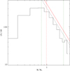 |
Fig. 14. Mass function of the disk-less and disk-bearing candidate members of Dolidze 25 (the latter considered only if inside the ACIS field). The vertical red lines mark the median mass value. The dashed black line is obtained from a linear fit in the log–log space on the mass distribution between 0.8 and 2 M⊙ (values marked with dotted green lines). The red line shows the normalized Salpeter–Kroupa IMF with α = 2.35 (Kroupa & Weidner 2003). |
7.4. Completeness
Estimating the completeness of our list of members, which was compiled by combining the outcome of several selection criteria that were different from each other, is an almost impossible task. We can still try to assess the fraction of real cluster members per magnitude bin that we missed to select by comparing the catalog of sources inside the field observed with ACIS with that in a control field.
In order to select the control field, we noted that the region in the south and southwest do not show any prominent nebular emission at 12 μm (see Fig. 1). We thus selected an annular region between 22 8 and 30
 6 from the center of the studied field and with δ ≤ −0.0876678, encompassing an area almost equal to that of the ACIS FoV. When we derived the magnitude distribution in a given bands, sources in this field whose error in the particular band is smaller than 0.1m form the “control” sample. We then selected all sources in the ACIS FoV that were not selected as members and whose error in the particular band was smaller than 0.1m. These sources are the “ACIS FoV” sample. The two samples should contain the same foreground population, while the background population at the faint end of the magnitude distributions is expected to be richer in the control field because the extinction is lower than in the ACIS FoV sample. The latter sample should also contain any member of Dolidze 25 that we missed to select, for instance, because of the strong variability in IR (Morales-Calderón et al. 2011) and X-ray (Stassun et al. 2007) bands that is typical of pre-main-sequence stars. The “members” sample instead contains all selected members whose error in the given magnitude is smaller than 0.1m.
Figure 15 shows the normalized magnitude distributions of the three samples at [3.6] and in the z Pan-STARRS bands. These two bands were selected because most of the members have good photometry in them (in particular, 82% and 77% of the members have errors smaller than 0.1m in [3.6] and zPanSTARRS, respectively). The [3.6] band is a useful test because the extinction effects are negligible. The fraction of missed members that can be estimated from the comparison between the control and ACIS FoV samples is about 3% at ∼15m and 5% at ∼16m. For fainter magnitudes, the intrinsic incompleteness of the IRAC catalog becomes dominant. Only at the faintest magnitude bin does the control sample become more numerous than the ACIS FoV sample because of the highly extinguished background population. Because the effect of extinction is stronger, the distributions of zPanSTARRS magnitudes are slightly more messy, but they suggest that the selection of members may be significantly incomplete for magnitudes fainter than 18m. We therefore consider the interval 13m ≤ zPanSTARRS ≤ 18m to be fairly complete. Appendix H shows the magnitude distributions of the three samples in the photometric bands we studied.
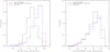 |
Fig. 15. Magnitude distribution at [3.6] and zPanSTARRS bands for the control, ACIS FoV, and members samples. |
7.5. Disk fraction
We can now calculate the disk fraction in Dolidze 25 considering the completeness of our sample. In the whole ACIS field we selected 222 stars with a disk and 424 members without a disk. To account for multiple matches, we counted all the candidate disk-less members with multiple OIR counterpart and the disk-bearing sources with multiple infrared counterparts. The resulting numbers are 218 and 384 for disk-bearing and disk-less stars, respectively, which means an average disk fraction of 34%±2%. When the populations of the central cluster and the northern rim are considered separately, the resulting disk fractions are 30%±3% and 43%±3%, respectively. This difference is expected from the presence of a slightly younger population along the rim and for the decline of sensitivity in the ACIS-I detector at large off-axis angles.
In the previous section we have found that our list is fairly complete in the zPanSTARRS magnitude range between 13m and 18m. In this magnitude range, the disk fraction is equal to 34%±4% (93 unique disk-less and 48 unique disk-bearing stars). Following the low-metallicity PARSEC isochrone at log(age) = 6.2 Myr, this magnitude range corresponds to stars more massive than 1.5 M⊙. However, Table 3 shows that the resulting value for the disk fraction does not strongly change when different cuts in stellar masses are adopted. When we only consider the mass intervals that result in an error in disk fraction smaller than 0.05, the values of the disk fraction range from 0.304 ± 0.041 to 0.364 ± 0.049.
Disk fraction resulting when different cuts in stellar masses are applied.
We can now compare the disk fraction of Dolidze 25 by adopting the value of 34% ± 4% with that of 58 other clusters younger than 10 Myr, which provides a wide range of star-forming environments. These clusters are listed in the table in Appendix G. The table provides their ages, distances, disk fractions, and references. When different estimates were available from different authors, we favored estimates based on selections of disk-bearing members from infrared photometry and/or disk-less members from X-ray observations or from proper motions or radial velocities. We mark the relevant publication in bold in Table G.1. Results are shown in Fig. 16, where we separately marked clusters closer than 1 kpc to the Sun, whose disk fraction estimate is expected to be less affected by incompleteness and whose metallicity is expected to be more similar to the solar values than those of more distant clusters; massive clusters in which evidence is found that supports a rapid dispersal of disks through massive stars or close stellar encounters; and low-metallicity clusters in the outer Galaxy. For the massive clusters we show an average value of the disk fraction, which is typically about 15%–20% higher than the values measured in the cluster core. The nearby clusters follow the well-known narrow decline of the disk fraction with age. The disk fraction in Dolidze 25 is more than 15%–20% lower than that of the nearby clusters with similar ages. We incidentally note that the disk fraction of Dolidze 25 is similar to that of the average value observed in coeval massive clusters with ages between 1 and 2 Myr, where externally induced photoevaporation and close encounters have induced a fast dispersal of protoplanetary disks, such as NGC 6611 (Guarcello et al. 2010a), CygnusOB2 (Guarcello et al. 2016), NGC 2244 (Balog et al. 2007), and Pismis24 (Fang et al. 2012). This comparison thus suggests that the disk dispersal in Dolidze 25 occurred faster on average than in coeval clusters within 1 kpc from the Sun. The timescales are similar to those occurring in massive clusters. Figure 16 also shows that the disk fraction observed in Dolidze 25 is larger than that found in the low-metallicity clusters in the outer Galaxy by Yasui et al. (2010). Two hypotheses may explain this discrepancy. The first hypothesis is the difficulty of obtaining a complete census of members of the distant young clusters still in the embedded phase in the outer Galaxy, and the second is a stronger metallicity effect throughout the disk dispersal timescale in the outer Galaxy. Future observations may help distinguish between these two possibilities.
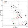 |
Fig. 16. Disk fraction vs. age of 58 clusters with ages between 0 and 10 Myr. Nearby clusters, e.g., closer than 1 kpc to the Sun, are marked with large black dots, massive clusters are marked with red dots, and the low-metallicity star-forming regions studied by Yasui et al. (2010) are plotted in green. The average estimate of the disk fraction in Dolidze 25 we obtained by accounting for completeness is marked with stars. |
7.6. Can O stars photoevaporate disks in Dolidze 25?
In this section we verify whether the dispersal timescale in Dolidze 25 may have been affected by externally induced photoevaporation. As explained in Sect. 1, photoevaporation can be induced externally by the UV radiation that is emitted by nearby massive stars. Dolidze 25 hosts ten OB stars (Moffat & Vogt 1975), only five of which are O stars: O6V star S33, O7V star S17, O7.5V star S15, and the two O9.7V stars S1 and S12. In order to estimate the intracluster UV field, we adopted the values corresponding to their spectral classes provided by Martins et al. (2005) as FUV and EUV fluxes emitted by these stars. We thus calculated the total FUV and EUV local field at the position of each selected cluster member by projecting and summing the contributions from these O stars. In this calculation, we used the projected distances from the cluster members to the O stars, which results in an overestimate of the real incident flux.
The resulting distributions of local UV fields at the positions of the candidate cluster members are shown in Fig. 17. By comparing these values with those for the members of the young cluster NGC 6611 (Fig. 15 in Guarcello et al. 2013), where the disk fraction only decreases in the cluster core that hosts about 50 OB stars (Hillenbrand et al. 1993), it is possible to verify that the intracluster UV field in Dolidze 25 is similar to that in the outskirts of NGC 6611, where no environmental effects on disk dispersal timescales are observed. The low disk fraction in Dolidze 25 is thus more likely a consequence of a faster dispersal of disks that is due to their low metallicity.
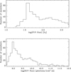 |
Fig. 17. Histogram of the FUV (top panel) and EUV (bottom panel) fields for the candidate member. The FUV fluxes are in units of the Habing flux G0, with 1 G0 = 1.6 × 10⁻³ erg cm−2 s−1 (1.7 G0 is equal to the average interstellar UV field in the solar neighborhood in the 912–2000 Å band, Habing 1968). The vast majority of candidate cluster members lies in areas of very low values of the local UV field. |
8. Conclusions
We have analyzed two specific Chandra ACIS-I observations (76.67 and 68.44 ks long) and archival data of the open cluster Dolidze 25 in order to calculate the disk fraction of the cluster and compare it with that of other clusters and associations younger than 10 Myr. Our work is motivated by the fact that Dolidze 25 is part of a star-forming region that counts among those with the lowest metallicity in the Galaxy (Lennon et al. 1990; Fitzsimmons et al. 1992; Negueruela et al. 2015). Protoplanetary disks in low-metallicity environments are expected to evolve on a different timescale than those formed in high-metallicity environments. However, the results obtained to date on the effects of metallicity on disk dispersal are quite controversial, notwithstanding the importance of this topic. For instance, any effect of metallicity on the disk dispersal timescale would mean that the disk evolution and planet formation in early epochs of our Galaxy, when the metallicity was lower than at present, was different than today.
On one hand, observational studies of star-forming regions in the outer Galaxy, characterized by very low metallicity, have demonstrated that disks can be dispersed very quickly, with a disk fraction ≤20% even at 1 Myr and almost zero after 2 Myr (Yasui et al. 2009, 2010, 2016a,b). The conclusions of these studies was a strong theoretical confirmation of the models presented by Ercolano & Clarke (2010). On the other hand, the selection of accreting disks older than 10 Myr in the Magellanic Clouds that was performed by several authors (Spezzi et al. 2012; De Marchi et al. 2010, 2017; Biazzo et al. 2019) suggests that accretion timescales can be longer, even though accretion rates are higher in low-metallicity environments. This might be due to several effects, such as a weaker effect of the radiation pressure on the inner disks in low-metallicity environments (De Marchi et al. 2017), or a lower disk temperature due to the lower dust opacity that results in longer accretion timescales (Durisen et al. 2007). It must be noted that the authors of these studies adopted different diagnostics to select young stars. In the observational works by Yasui and collaborators, disks were selected from near-infrared (NIR) photometry and are therefore sensitive to the micron-size dust emission from disks, while the studies on the Magellanic Clouds are based on photometric evidence of accretion in disks, which were not selected in the infrared, however.
We have compiled a multiband catalog of the sources within 0.5 deg from Dolidze 25 by combining the X-ray catalog with an extensive list of available optical and infrared catalogs of the region: VPHAS+, IPHAS, Pan-STARRS, the optical catalog published by Delgado et al. (2010), Gaia DR2 and EDR3, CoRoT, LAMOST, 2MASS PSC, UKIDSS DR10, the Spitzer-IRAC catalog obtained by Puga et al. (2009), and the AllWISE Source Catalog. The catalogs were combined by adopting a close-neighborhood approach or a maximum likelihodd approach, in the latter case considering available photometry together with the angular separation between sources of the various catalogs. Multiple coincidences, false positives, and false negatives resulting from the matching procedure were properly treated in order to reduce their effect on the final multiband catalog, which contains 101 722 entries.
We selected 667 disk-bearing stars that populate different recent star-forming sites of Sh2-284 that were previously discovered by Puga et al. (2009): together with Dolidze 25 at the center of the cavity, we studied the clusters Cl2 and Cl3 and the bright-rimmed clouds RN, RS, and RE. These stars were selected by adopting criteria based on the Spitzer-IRAC, WISE, and JHK colors, together with specific criteria defined in order to select and discard foreground and background contaminants. Inside the ACIS FoV, centered on Dolidze 25, we found 222 stars with a disk. The disk-less population of Dolidze 25 (424 sources) was instead selected from the 618 sources detected in X-rays, discarding those without optical or infrared counterpart, which are expected to be strongly contaminated by extragalactic sources, and X-ray+OIR sources with optical and infrared colors typical of foreground and background sources.
The spatial distribution of the candidate young stars associated with Dolidze 25 and Sh2-284 confirms the existence of multiple regions in the area and does not support the presence of mass segregation. The main concentrations in the central cavity are Dolidze 25 and the young stars associated with the northern rim of the cavity that is cleared by the cluster itself. We derived an extinction map of the whole area and verified that an average difference of less than 1 mag of extinction exists between the central and the northern regions of the cavity. We estimated masses and ages of the candidate members. We do not find convincing evidence that would support a deviation of the IMF in Dolidze 25 from the universal slope due to the low metallicity of the cluster. We also estimated the median age of the cluster equal to log(age)median = 6.2 Myr, with a standard deviation of 0.3 Myr.
Our estimate of the disk fraction of the cluster slightly changes when different selections are adopted that aim to minimize the incompleteness effects. We adopted an average value of ∼34%. By collecting the estimate of the disk fractions of 58 clusters and associations younger than 10 Myr, we found evidence supporting a lower disk fraction of Dolidze 25 than in star-forming environments with solar metallicity and similar age. In particular, the disk fraction in Dolidze 25 is similar to the fractions found in massive clusters, where disk dispersal in the proximity of massive stars is accelerated by the externally induced disk photoevaporation. Because the massive population of Dolidze 25 (counting only five O-late stars) does not produce an intracluster UV field intense enough to induce disk photoevaporation, this difference is more likely due to the low metallicity of the cluster and not to other environment feedback.
Our conclusions depend on the reliability of the age estimate of the cluster. We estimated stellar ages by fitting suitable isochrones to the distribution of cluster members in color-magnitude diagrams. This procedure can be affected by large uncertainties, and it also depends on the reliability of the adopted models to describe the pre-main-sequence phase. This can have a strong effect on our conclusions: For instance, with a mean cluster age of 3 Myr rather than 1.2 Myr, our estimate of disk fraction would be similar to those of the other clusters. Bearing this caveat in mind, we claim that the disk fraction in Dolidze 25 is likely to be affected by the low metallicity of this star-forming region.
The ACIS Extract software package and User’s Guide are available online at http://personal.psu.edu/psb6/TARA/AE.html.
With the SED fitting as a test, we attempted to break the degeneracy between highly extinguished background giants with circumstellar dust and stars with a disk showing infrared excesses at the longest wavelength.
Acknowledgments
The authors acknowledge the referee for his/hers comments and careful reading of our manuscript, that helped us improving our paper. KB has been supported by the project PRIN-INAF-MAIN-STREAM 2018 “Protoplanetary disks seen through the eyes of new-generation instruments”. This work is based on: VPHAS+ data, which are based on observations made with ESO Telescopes at the La Silla or Paranal Observatories under programme ID(s) 177.D-3023(B), 177.D-3023(C), 177.D-3023(D), 177.D-3023(E); IPHAS data, obtained from observations (www.iphas.org) carried out at the Isaac Newton Telescope (INT), operating on the island of La Palma by the Isaac Newton Group in the Spanish Observatorio del Roque de los Muchachos of the Instituto de Astrofisica de Canarias; data from the Pan-STARRS1 Surveys (PS1), which have been made possible through contributions by the Institute for Astronomy, the University of Hawaii, the Pan-STARRS Project Office, the Max-Planck Society and its participating institutes, the Max Planck Institute for Astronomy, Heidelberg and the Max Planck Institute for Extraterrestrial Physics, Garching, The Johns Hopkins University, Durham University, the University of Edinburgh, the Queen’s University Belfast, the Harvard-Smithsonian Center for Astrophysics, the Las Cumbres Observatory Global Telescope Network Incorporated, the National Central University of Taiwan, the Space Telescope Science Institute, and the National Aeronautics and Space Administration under Grant No. NNX08AR22G issued through the Planetary Science Division of the NASA Science Mission Directorate, the National Science Foundation Grant No. AST-1238877, the University of Maryland, Eotvos Lorand University (ELTE), and the Los Alamos National Laboratory; data from the European Space Agency (ESA) mission Gaia (https://www.cosmos.esa.int/gaia), processed by the Gaia Data Processing and Analysis Consortium (DPAC, https://www.cosmos.esa.int/web/gaia/dpac/consortium), with funds provided by national institutions, in particular the institutions participating in the Gaia Multilateral Agreement; data products from the Two Micron All Sky Survey, which is a joint project of the University of Massachusetts and the Infrared Processing and Analysis Center, California Institute of Technology, funded by the National Aeronautics and Space Administration and the National Science Foundation; data obtained as part of the UKIRT Infrared Deep Sky Survey; data from observations made with the Spitzer Space Telescope, which was operated by the Jet Propulsion Laboratory, California Institute of Technology under a contract with NASA; data products from the Wide-field Infrared Survey Explorer, which is a joint project of the University of California, Los Angeles, and the Jet Propulsion Laboratory/California Institute of Technology, funded by the National Aeronautics and Space Administration. The authors also acknowledge the use of the TOPCAT software, described in Taylor (2005), and the VizieR catalogue access tool, CDS, Strasbourg, France (DOI: 10.26093/cds/vizier), described in Ochsenbein et al. (2000).
References
- Affer, L., Micela, G., Favata, F., & Flaccomio, E. 2012, MNRAS, 424, 11 [NASA ADS] [CrossRef] [Google Scholar]
- Alcalá, J. M., Spezzi, L., Chapman, N., et al. 2008, ApJ, 676, 427 [Google Scholar]
- Allen, T. S., Gutermuth, R. A., Kryukova, E., et al. 2012, ApJ, 750, 125 [NASA ADS] [CrossRef] [Google Scholar]
- Allison, R. J., Goodwin, S. P., Parker, R. J., et al. 2009, MNRAS, 395, 1449 [Google Scholar]
- Armitage, P. J., Clarke, C. J., & Palla, F. 2003, MNRAS, 342, 1139 [NASA ADS] [CrossRef] [Google Scholar]
- Baglin, A., Auvergne, M., Barge, P., et al. 2006, in The CoRoT Mission Pre-Launch Status - Stellar Seismology and Planet Finding, eds. M. Fridlund, A. Baglin, J. Lochard, & L. Conroy, ESA Special Publ., 1306, 33 [Google Scholar]
- Bai, X.-N., & Stone, J. M. 2013, ApJ, 769, 76 [Google Scholar]
- Bai, X.-N., Ye, J., Goodman, J., & Yuan, F. 2016, ApJ, 818, 152 [Google Scholar]
- Bailer-Jones, C. A. L., Rybizki, J., Fouesneau, M., Mantelet, G., & Andrae, R. 2018, AJ, 156, 58 [NASA ADS] [CrossRef] [Google Scholar]
- Balbus, S. A., & Hawley, J. F. 1991, ApJ, 376, 214 [NASA ADS] [CrossRef] [Google Scholar]
- Bally, J., O’Dell, C. R., & McCaughrean, M. J. 2000, AJ, 119, 2919 [NASA ADS] [CrossRef] [Google Scholar]
- Balog, Z., Rieke, G. H., Su, K. Y. L., Muzerolle, J., & Young, E. T. 2006, ApJ, 650, L83 [NASA ADS] [CrossRef] [Google Scholar]
- Balog, Z., Muzerolle, J., Rieke, G. H., et al. 2007, ApJ, 660, 1532 [NASA ADS] [CrossRef] [Google Scholar]
- Barentsen, G., Vink, J. S., Drew, J. E., et al. 2011, MNRAS, 415, 103 [NASA ADS] [CrossRef] [Google Scholar]
- Barentsen, G., Farnhill, H. J., Drew, J. E., et al. 2014, MNRAS, 444, 3230 [NASA ADS] [CrossRef] [Google Scholar]
- Barrow, J. D., Bhavsar, S. P., & Sonoda, D. H. 1985, MNRAS, 216, 17 [NASA ADS] [CrossRef] [MathSciNet] [Google Scholar]
- Baume, G., Vázquez, R. A., & Feinstein, A. 1999, A&AS, 137, 233 [NASA ADS] [CrossRef] [EDP Sciences] [Google Scholar]
- Beccari, G., De Marchi, G., Panagia, N., et al. 2015, A&A, 574, A44 [NASA ADS] [CrossRef] [EDP Sciences] [Google Scholar]
- Biazzo, K., Beccari, G., De Marchi, G., & Panagia, N. 2019, ApJ, 875, 51 [Google Scholar]
- Bik, A., Stolte, A., Gennaro, M., et al. 2014, A&A, 561, A12 [NASA ADS] [CrossRef] [EDP Sciences] [Google Scholar]
- Brescia, M., Cavuoti, S., & Longo, G. 2015, MNRAS, 450, 3893 [NASA ADS] [CrossRef] [Google Scholar]
- Bressan, A., Marigo, P., Girardi, L., et al. 2012, MNRAS, 427, 127 [NASA ADS] [CrossRef] [Google Scholar]
- Briceño, C. 2009, Rev. Mex. Astron. Astrofis. Conf. Ser., 35, 27 [Google Scholar]
- Briceño, C., Hartmann, L., Hernández, J., et al. 2007, ApJ, 661, 1119 [NASA ADS] [CrossRef] [Google Scholar]
- Broos, P. S., Townsley, L. K., Feigelson, E. D., et al. 2010, ApJ, 714, 1582 [NASA ADS] [CrossRef] [Google Scholar]
- Calvet, N., & Gullbring, E. 1998, ApJ, 509, 802 [NASA ADS] [CrossRef] [Google Scholar]
- Cardelli, J. A., Clayton, G. C., & Mathis, J. S. 1989, ApJ, 345, 245 [NASA ADS] [CrossRef] [Google Scholar]
- Carone, L., Gandolfi, D., Cabrera, J., et al. 2012, A&A, 538, A112 [NASA ADS] [CrossRef] [EDP Sciences] [Google Scholar]
- Carpenter, J. M., Mamajek, E. E., Hillenbrand, L. A., & Meyer, M. R. 2006, ApJ, 651, L49 [NASA ADS] [CrossRef] [Google Scholar]
- Chambers, K. C., Magnier, E. A., Metcalfe, N., et al. 2016, ArXiv e-prints [arXiv:1612.05560] [Google Scholar]
- Clarke, C. J., & Pringle, J. E. 1993, MNRAS, 261, 190 [Google Scholar]
- COROT Team 2016, VizieR Online Data Catalog: B/corot [Google Scholar]
- Cusano, F., Ripepi, V., Alcalá, J. M., et al. 2011, MNRAS, 410, 227 [NASA ADS] [CrossRef] [Google Scholar]
- Cutri, R. M. 2012, VizieR Online Data Catalog: II/311 [Google Scholar]
- Cutri, R. M., Skrutskie, M. F., van Dyk, S., et al. 2003, VizieR Online Data Catalog: II/246 [Google Scholar]
- Dahm, S. E., & Hillenbrand, L. A. 2007, AJ, 133, 2072 [NASA ADS] [CrossRef] [Google Scholar]
- Damiani, F., Maggio, A., Micela, G., & Sciortino, S. 1997, ApJ, 483, 350 [NASA ADS] [CrossRef] [Google Scholar]
- Damiani, F., Prisinzano, L., Micela, G., & Sciortino, S. 2006, A&A, 459, 477 [NASA ADS] [CrossRef] [EDP Sciences] [Google Scholar]
- Damiani, F., Micela, G., & Sciortino, S. 2016, A&A, 596, A82 [NASA ADS] [CrossRef] [EDP Sciences] [Google Scholar]
- Debosscher, J., Sarro, L. M., López, M., et al. 2009, A&A, 506, 519 [NASA ADS] [CrossRef] [EDP Sciences] [Google Scholar]
- Delgado, A. J., Djupvik, A. A., & Alfaro, E. J. 2010, A&A, 509, A104 [NASA ADS] [CrossRef] [EDP Sciences] [Google Scholar]
- De Marchi, G., Panagia, N., & Romaniello, M. 2010, ApJ, 715, 1 [NASA ADS] [CrossRef] [Google Scholar]
- De Marchi, G., Panagia, N., Romaniello, M., et al. 2011, ApJ, 740, 11 [NASA ADS] [CrossRef] [Google Scholar]
- De Marchi, G., Panagia, N., & Beccari, G. 2017, ApJ, 846, 110 [CrossRef] [Google Scholar]
- Drew, J. E., Greimel, R., Irwin, M. J., et al. 2005, MNRAS, 362, 753 [NASA ADS] [CrossRef] [Google Scholar]
- Drew, J. E., Gonzalez-Solares, E., Greimel, R., et al. 2014, MNRAS, 440, 2036 [NASA ADS] [CrossRef] [Google Scholar]
- Drew, J. E., Gonzalez-Solares, E., Greimel, R., et al. 2016, VizieR Online Data Catalog: II/341 [Google Scholar]
- Dullemond, C. P., & Dominik, C. 2005, A&A, 434, 971 [NASA ADS] [CrossRef] [EDP Sciences] [Google Scholar]
- Durisen, R. H., Boss, A. P., Mayer, L., et al. 2007, in Protostars and Planets V, eds. B. Reipurth, D. Jewitt, & K. Keil, 607 [Google Scholar]
- Dutta, S., Mondal, S., Jose, J., et al. 2015, MNRAS, 454, 3597 [CrossRef] [Google Scholar]
- Ercolano, B., & Clarke, C. J. 2010, MNRAS, 402, 2735 [NASA ADS] [CrossRef] [Google Scholar]
- Ercolano, B., Drake, J. J., Raymond, J. C., & Clarke, C. C. 2008, ApJ, 688, 398 [NASA ADS] [CrossRef] [Google Scholar]
- Ercolano, B., Clarke, C. J., & Drake, J. J. 2009, ApJ, 699, 1639 [NASA ADS] [CrossRef] [Google Scholar]
- Esteban, C., Carigi, L., Copetti, M. V. F., et al. 2013, MNRAS, 433, 382 [NASA ADS] [CrossRef] [Google Scholar]
- Fang, M., van Boekel, R., King, R. R., et al. 2012, A&A, 539, A119 [NASA ADS] [CrossRef] [EDP Sciences] [Google Scholar]
- Fang, M., Kim, J. S., van Boekel, R., et al. 2013, ApJS, 207, 5 [NASA ADS] [CrossRef] [Google Scholar]
- Fang, M., Kim, J. S., Pascucci, I., Apai, D., & Manara, C. F. 2016, ApJ, 833, L16 [NASA ADS] [CrossRef] [Google Scholar]
- Feigelson, E. D., Townsley, L. K., Broos, P. S., et al. 2013, ApJS, 209, 26 [Google Scholar]
- Fischer, D. A., & Valenti, J. 2005, ApJ, 622, 1102 [Google Scholar]
- Fitzsimmons, A., Dufton, P. L., & Rolleston, W. R. J. 1992, MNRAS, 259, 489 [NASA ADS] [CrossRef] [Google Scholar]
- Flaherty, K. M., & Muzerolle, J. 2008, AJ, 135, 966 [NASA ADS] [CrossRef] [Google Scholar]
- Freeman, P. E., Kashyap, V., Rosner, R., & Lamb, D. Q. 2002, ApJs, 138, 185 [NASA ADS] [CrossRef] [Google Scholar]
- Fruscione, A., McDowell, J. C., Allen, G. E., et al. 2006, Proc. SPIE, 6270, 62701V [Google Scholar]
- Gaia Collaboration (Prusti, T., et al.) 2016, A&A, 595, A1 [NASA ADS] [CrossRef] [EDP Sciences] [Google Scholar]
- Galli, P. A. B., Loinard, L., Bouy, H., et al. 2019, A&A, 630, A137 [NASA ADS] [CrossRef] [EDP Sciences] [Google Scholar]
- Gorti, U., & Hollenbach, D. 2009, ApJ, 690, 1539 [Google Scholar]
- Guarcello, M. G., Prisinzano, L., Micela, G., et al. 2007, A&A, 462, 245 [NASA ADS] [CrossRef] [EDP Sciences] [Google Scholar]
- Guarcello, M. G., Micela, G., Damiani, F., et al. 2009, A&A, 496, 453 [NASA ADS] [CrossRef] [EDP Sciences] [Google Scholar]
- Guarcello, M. G., Micela, G., Peres, G., Prisinzano, L., & Sciortino, S. 2010a, A&A, 521, A61 [NASA ADS] [CrossRef] [EDP Sciences] [Google Scholar]
- Guarcello, M. G., Damiani, F., Micela, G., et al. 2010b, A&A, 521, A18 [NASA ADS] [CrossRef] [EDP Sciences] [Google Scholar]
- Guarcello, M. G., Drake, J. J., Wright, N. J., et al. 2013, ApJ, 773, 135 [NASA ADS] [CrossRef] [Google Scholar]
- Guarcello, M. G., Drake, J. J., Wright, N. J., García-Alvarez, D., & Kraemer, K. E. 2014, ApJ, 793, 56 [NASA ADS] [CrossRef] [Google Scholar]
- Guarcello, M. G., Drake, J. J., Wright, N. J., et al. 2015, ArXiv e-prints [arXiv:1501.03761] [Google Scholar]
- Guarcello, M. G., Drake, J. J., Wright, N. J., et al. 2016, ArXiv e-prints[arXiv:1605.01773] [Google Scholar]
- Guenther, E. W., Gandolfi, D., Sebastian, D., et al. 2012, A&A, 543, A125 [NASA ADS] [CrossRef] [EDP Sciences] [Google Scholar]
- Gutermuth, R. A., Megeath, S. T., Myers, P. C., et al. 2009, ApJS, 184, 18 [NASA ADS] [CrossRef] [Google Scholar]
- Habing, H. J. 1968, Bull. Astron. Inst. Neth., 19, 421 [Google Scholar]
- Haisch, K. E., Jr, Lada, E. A., & Lada, C. J. 2001, ApJ, 553, L153 [NASA ADS] [CrossRef] [Google Scholar]
- Hartmann, L. 2009, Accretion Processes in Star Formation, 2nd edn. (Cambridge: Cambridge University Press) [Google Scholar]
- Hartmann, L., D’Alessio, P., Calvet, N., & Muzerolle, J. 2006, ApJ, 648, 484 [Google Scholar]
- Helled, R., Bodenheimer, P., Podolak, M., et al. 2014, in Protostars and Planets VI, eds. H. Beuther, R. S. Klessen, C. P. Dullemond, & T. Henning, 643 [Google Scholar]
- Hernández, J., Hartmann, L., Megeath, T., et al. 2007, ApJ, 662, 1067 [NASA ADS] [CrossRef] [Google Scholar]
- Hernández, J., Hartmann, L., Calvet, N., et al. 2008, ApJ, 686, 1195 [NASA ADS] [CrossRef] [Google Scholar]
- Hernández, J., Morales-Calderon, M., Calvet, N., et al. 2010, ApJ, 722, 1226 [NASA ADS] [CrossRef] [Google Scholar]
- Hillenbrand, L. A., Massey, P., Strom, S. E., & Merrill, K. M. 1993, AJ, 106, 1906 [NASA ADS] [CrossRef] [Google Scholar]
- Hubickyj, O., Bodenheimer, P., & Lissauer, J. J. 2005, Icarus, 179, 415 [NASA ADS] [CrossRef] [Google Scholar]
- Jeffries, R. D., Jackson, R. J., Franciosini, E., et al. 2017, MNRAS, 464, 1456 [NASA ADS] [CrossRef] [Google Scholar]
- Johnstone, D., Hollenbach, D., & Bally, J. 1998, ApJ, 499, 758 [NASA ADS] [CrossRef] [Google Scholar]
- Jose, J., Kim, J. S., Herczeg, G. J., et al. 2016, ApJ, 822, 49 [NASA ADS] [CrossRef] [Google Scholar]
- Kalari, V. M., & Vink, J. S. 2015, ApJ, 800, 113 [NASA ADS] [CrossRef] [Google Scholar]
- Kim, J. S., Clarke, C. J., Fang, M., & Facchini, S. 2016, ApJ, 826, L15 [NASA ADS] [CrossRef] [Google Scholar]
- Koenig, X. P., & Leisawitz, D. T. 2014, ApJ, 791, 131 [NASA ADS] [CrossRef] [Google Scholar]
- Kounkel, M., Covey, K., Suárez, G., et al. 2018, AJ, 156, 84 [NASA ADS] [CrossRef] [Google Scholar]
- Kraus, A. L., Herczeg, G. J., Rizzuto, A. C., et al. 2017, ApJ, 838, 150 [NASA ADS] [CrossRef] [Google Scholar]
- Kroupa, P., & Weidner, C. 2003, ApJ, 598, 1076 [NASA ADS] [CrossRef] [Google Scholar]
- Lada, C. J., Muench, A. A., Luhman, K. L., et al. 2006, AJ, 131, 1574 [Google Scholar]
- Lawrence, A., Warren, S. J., Almaini, O., et al. 2007, MNRAS, 379, 1599 [NASA ADS] [CrossRef] [MathSciNet] [Google Scholar]
- Lennon, D. J., Dufton, P. L., Fitzsimmons, A., Gehren, T., & Nissen, P. E. 1990, A&A, 240, 349 [NASA ADS] [Google Scholar]
- Luhman, K. L., & Mamajek, E. E. 2012, ApJ, 758, 31 [NASA ADS] [CrossRef] [Google Scholar]
- Luo, A.-L., Zhao, Y.-H., Zhao, G., et al. 2015, Res. Astron. Astrophys., 15, 1095 [NASA ADS] [CrossRef] [Google Scholar]
- Luo, A. L., Zhao, Y. H., Zhao, G., et al. 2016, VizieR Online Data Catalog: V/149 [Google Scholar]
- Maeder, A., Grebel, E. K., & Mermilliod, J.-C. 1999, A&A, 346, 459 [NASA ADS] [Google Scholar]
- Manzo-Martínez, E., Calvet, N., Hernández, J., et al. 2020, ApJ, 893, 56 [CrossRef] [Google Scholar]
- Mariñas, N., Lada, E. A., Teixeira, P. S., & Lada, C. J. 2013, ApJ, 772, 81 [NASA ADS] [CrossRef] [Google Scholar]
- Martins, F., Schaerer, D., & Hillier, D. J. 2005, A&A, 436, 1049 [NASA ADS] [CrossRef] [EDP Sciences] [Google Scholar]
- Megeath, S. T., Hartmann, L., Luhman, K. L., & Fazio, G. G. 2005, ApJ, 634, L113 [NASA ADS] [CrossRef] [Google Scholar]
- Merín, B., Jørgensen, J., Spezzi, L., et al. 2008, ApJS, 177, 551 [Google Scholar]
- Mesa-Delgado, A., Zapata, L., Henney, W. J., Puzia, T. H., & Tsamis, Y. G. 2016, ApJ, 825, L16 [NASA ADS] [CrossRef] [Google Scholar]
- Moffat, A. F. J., & Vogt, N. 1975, A&AS, 20, 85 [NASA ADS] [Google Scholar]
- Montmerle, T. 1996, in Cool Stars, Stellar Systems, and the Sun, eds. R. Pallavicini, & A. K. Dupree, ASP Conf. Ser., 109, 405 [NASA ADS] [Google Scholar]
- Morales-Calderón, M., Stauffer, J. R., Hillenbrand, L. A., et al. 2011, ApJ, 733, 50 [NASA ADS] [CrossRef] [Google Scholar]
- Muzerolle, J., Hartmann, L., & Calvet, N. 1998, AJ, 116, 455 [Google Scholar]
- Nakatani, R., Hosokawa, T., Yoshida, N., Nomura, H., & Kuiper, R. 2018a, ApJ, 857, 57 [CrossRef] [Google Scholar]
- Nakatani, R., Hosokawa, T., Yoshida, N., Nomura, H., & Kuiper, R. 2018b, ApJ, 865, 75 [NASA ADS] [CrossRef] [Google Scholar]
- Negueruela, I., Simón-Díaz, S., Lorenzo, J., Castro, N., & Herrero, A. 2015, A&A, 584, A77 [NASA ADS] [CrossRef] [EDP Sciences] [Google Scholar]
- Ochsenbein, F., Bauer, P., & Marcout, J. 2000, A&AS, 143, 23 [NASA ADS] [CrossRef] [EDP Sciences] [Google Scholar]
- O’dell, C. R., & Wen, Z. 1994, ApJ, 436, 194 [NASA ADS] [CrossRef] [Google Scholar]
- O’Donnell, J. E. 1994, ApJ, 422, 158 [NASA ADS] [CrossRef] [Google Scholar]
- Olczak, C., Kaczmarek, T., Harfst, S., Pfalzner, S., & Portegies Zwart, S. 2012, ApJ, 756, 123 [NASA ADS] [CrossRef] [Google Scholar]
- Paradis, E., & Schliep, K. 2018, Bioinformatics, 35, 526 [CrossRef] [Google Scholar]
- Park, B.-G., & Sung, H. 2002, AJ, 123, 892 [NASA ADS] [CrossRef] [Google Scholar]
- Pecaut, M. J., & Mamajek, E. E. 2016, MNRAS, 461, 794 [Google Scholar]
- Pfalzner, S., Umbreit, S., & Henning, T. 2005, ApJ, 629, 526 [NASA ADS] [CrossRef] [Google Scholar]
- Pizzolato, N., Ventura, P., D’Antona, F., et al. 2001, A&A, 373, 597 [NASA ADS] [CrossRef] [EDP Sciences] [Google Scholar]
- Pollack, J. B., Hubickyj, O., Bodenheimer, P., et al. 1996, Icarus, 124, 62 [NASA ADS] [CrossRef] [Google Scholar]
- Prisinzano, L., Sanz-Forcada, J., Micela, G., et al. 2011, A&A, 527, A77 [NASA ADS] [CrossRef] [EDP Sciences] [Google Scholar]
- Puga, E., Hony, S., Neiner, C., et al. 2009, A&A, 503, 107 [NASA ADS] [CrossRef] [EDP Sciences] [Google Scholar]
- Rafferty, D. A., Brandt, W. N., Alexander, D. M., et al. 2011, ApJ, 742, 3 [NASA ADS] [CrossRef] [Google Scholar]
- Rapson, V. A., Pipher, J. L., Gutermuth, R. A., et al. 2014, ApJ, 794, 124 [NASA ADS] [CrossRef] [EDP Sciences] [Google Scholar]
- Reiter, M., & Parker, R. J. 2019, MNRAS, 486, 4354 [CrossRef] [Google Scholar]
- Ribas, Á., Merín, B., Bouy, H., & Maud, L. T. 2014, A&A, 561, A54 [NASA ADS] [CrossRef] [EDP Sciences] [Google Scholar]
- Richert, A. J. W., Feigelson, E. D., Getman, K. V., & Kuhn, M. A. 2015, ApJ, 811, 10 [NASA ADS] [CrossRef] [Google Scholar]
- Richert, A. J. W., Getman, K. V., Feigelson, E. D., et al. 2018, MNRAS, 477, 5191 [NASA ADS] [CrossRef] [Google Scholar]
- Robitaille, T. P. 2017, A&A, 600, A11 [NASA ADS] [CrossRef] [EDP Sciences] [Google Scholar]
- Roccatagliata, V., Bouwman, J., Henning, T., et al. 2011, ApJ, 733, 113 [NASA ADS] [CrossRef] [Google Scholar]
- Rolleston, W. R. J., Smartt, S. J., Dufton, P. L., & Ryans, R. S. I. 2000, A&A, 363, 537 [NASA ADS] [Google Scholar]
- Rugel, M., Fedele, D., & Herczeg, G. 2018, A&A, 609, A70 [NASA ADS] [CrossRef] [EDP Sciences] [Google Scholar]
- Sebastian, D., Guenther, E. W., Schaffenroth, V., et al. 2012, A&A, 541, A34 [NASA ADS] [CrossRef] [EDP Sciences] [Google Scholar]
- Sharpless, S. 1959, ApJs, 4, 257 [NASA ADS] [CrossRef] [Google Scholar]
- Sicilia-Aguilar, A., Hartmann, L., Calvet, N., et al. 2006a, ApJ, 638, 897 [NASA ADS] [CrossRef] [Google Scholar]
- Sicilia-Aguilar, A., Hartmann, L. W., Fürész, G., et al. 2006b, AJ, 132, 2135 [NASA ADS] [CrossRef] [Google Scholar]
- Simon, J. B., Bai, X.-N., Armitage, P. J., Stone, J. M., & Beckwith, K. 2013, ApJ, 775, 73 [NASA ADS] [CrossRef] [Google Scholar]
- Smith, D. J. B., Dunne, L., Maddox, S. J., et al. 2011, MNRAS, 416, 857 [NASA ADS] [CrossRef] [Google Scholar]
- Spezzi, L., de Marchi, G., Panagia, N., Sicilia-Aguilar, A., & Ercolano, B. 2012, MNRAS, 421, 78 [Google Scholar]
- Spezzi, L., Petr-Gotzens, M. G., Alcalá, J. M., et al. 2015, A&A, 581, A140 [NASA ADS] [CrossRef] [EDP Sciences] [Google Scholar]
- Stassun, K. G., van den Berg, M., & Feigelson, E. 2007, ApJ, 660, 704 [NASA ADS] [CrossRef] [Google Scholar]
- Steinhausen, M., & Pfalzner, S. 2014, A&A, 565, A32 [NASA ADS] [CrossRef] [EDP Sciences] [Google Scholar]
- Stelzer, B., & Scholz, A. 2009, A&A, 507, 227 [NASA ADS] [CrossRef] [EDP Sciences] [Google Scholar]
- Stern, D., Eisenhardt, P., Gorjian, V., et al. 2005, ApJ, 631, 163 [NASA ADS] [CrossRef] [Google Scholar]
- Sung, H., Stauffer, J. R., & Bessell, M. S. 2009, AJ, 138, 1116 [NASA ADS] [CrossRef] [Google Scholar]
- Sung, H., Sana, H., & Bessell, M. S. 2013, AJ, 145, 37 [NASA ADS] [CrossRef] [Google Scholar]
- Suzuki, T. K., Muto, T., & Inutsuka, S.-I. 2010, ApJ, 718, 1289 [NASA ADS] [CrossRef] [Google Scholar]
- Taylor, M. B. 2005, in Astronomical Data Analysis Software and Systems XIV, eds. P. Shopbell, M. Britton, & R. Ebert, ASP Conf. Ser., 347, 29 [Google Scholar]
- Thies, I., Kroupa, P., Goodwin, S. P., Stamatellos, D., & Whitworth, A. P. 2010, ApJ, 717, 577 [Google Scholar]
- Treister, E., Urry, C. M., Van Duyne, J., et al. 2006, ApJ, 640, 603 [NASA ADS] [CrossRef] [Google Scholar]
- Turbide, L., & Moffat, A. F. J. 1993, AJ, 105, 1831 [NASA ADS] [CrossRef] [Google Scholar]
- Usatov, M. 2018, J. Astron. Data, 24, 3 [Google Scholar]
- Vincke, K., Breslau, A., & Pfalzner, S. 2015, A&A, 577, A115 [NASA ADS] [CrossRef] [EDP Sciences] [Google Scholar]
- Wang, J., Townsley, L. K., Feigelson, E. D., et al. 2008, ApJ, 675, 464 [NASA ADS] [CrossRef] [Google Scholar]
- Weidner, C., Kroupa, P., & Bonnell, I. A. D. 2010, MNRAS, 401, 275 [NASA ADS] [CrossRef] [Google Scholar]
- Winston, E., Megeath, S. T., Wolk, S. J., et al. 2007, ApJ, 669, 493 [NASA ADS] [CrossRef] [Google Scholar]
- Wright, E. L., Eisenhardt, P. R. M., Mainzer, A. K., et al. 2010, AJ, 140, 1868 [Google Scholar]
- Wright, N. J., Drake, J. J., Drew, J. E., et al. 2012, ApJ, 746, L21 [NASA ADS] [CrossRef] [Google Scholar]
- Wright, N. J., Drake, J. J., Guarcello, M. G., et al. 2014, ArXiv e-prints [arXiv:1408.6579] [Google Scholar]
- Yasui, C., Kobayashi, N., Tokunaga, A. T., Saito, M., & Tokoku, C. 2009, ApJ, 705, 54 [NASA ADS] [CrossRef] [Google Scholar]
- Yasui, C., Kobayashi, N., Tokunaga, A. T., Saito, M., & Tokoku, C. 2010, ApJ, 723, L113 [NASA ADS] [CrossRef] [Google Scholar]
- Yasui, C., Kobayashi, N., Saito, M., & Izumi, N. 2016a, AJ, 151, 115 [CrossRef] [Google Scholar]
- Yasui, C., Kobayashi, N., Tokunaga, A. T., Saito, M., & Izumi, N. 2016b, AJ, 151, 50 [CrossRef] [Google Scholar]
Appendix A: Catalog of X-ray sources in Dolidze 25
In this appendix we describe the catalog of X-ray sources in Dolidze 25.
X-ray catalog of Dolidze 25.
Appendix B: Multiwavelength catalog and the merging process
In this appendix, we describe the merging process we adopted to compile the multiwavelength catalog. We merged the catalogs two by two, defining a “master” catalog in each step that was matched with a “slave” catalog. Before merging, the astrometry of each catalog was anchored in the Gaia astrometry by matching them with a close-neighbors approach, adopting a radius of 5″, and then correcting for the median of the differences of the celestial coordinates of the matched sources. Table B.1 shows each step of the merging sequence together with other useful information: The matched catalogs and the name of the output catalog, the number of matched sources, the expected number of spurious coincidences, the initial number of multiple matches, and the resolved multiple coincidences after a visual inspection (see below). We adopted two merging methods: a close-neighbors approach, in which we searched for and merged the pairs of sources in the two catalogs separated by a spatial offset smaller than a given tolerance (the matching radius rmatch), and a maximum likelihood (ML) method, adapting to our case the algorithm described in Smith et al. (2011).
In the close-neighbors method, the matching radius is fixed by analyzing how the expected number of false positives grows as a function of the matching radius. If the stars in the catalogs were uniformly distributed within the area, the number of spurious coincidences could be calculated easily as Nsp = NmasterNslave × Amatch/Atotal, where Nmaster and Nslave are the number of master and slave sources, respectively, while Amatch/Atotal is the ratio between the matching area  over the area covered by the catalogs. This is not our case (see Fig. 6). We thus estimated the number of expected false positives by rigidly shifting the slave catalog in four directions by 5′. In this way, we randomized the slave catalog and kept the information of the spatial distribution of the slave sources. We then merged the master and the four randomized slave catalogs adopting a set of increasing rmatch. For each value of the matching radius, we took the mean number of matches obtained with the four randomized slave catalogs. As an example, in Fig. B.1 we show how in step 10 the distribution of total (Ntotal), spurious (Nspurious), and real (Nreal) coincidences varies as a function of the matching radius. The y-axis shows the differential increment of the coincidences (e.g., the difference between the number of matches obtained with the given rmatch with those obtained with the previous matching radius). In this case, for rmatch between 0
 6 and 0
 7, the increment of the estimated values of Nspurious is comparable with that of the expected real matches Nreal = Ntotal − Nspurious, which motivated our choice of fixing
  .
.
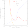 |
Fig. B.1. Distribution of total (Ntotal), spurious (Nspurious), and real (Nreal) coincidences in the match of the optical and the infrared catalogs. The distribution of Nspurious becomes comparable to that of Nreal for rmatch between 0 |


The close-neighbors method can fail when one of the two catalogs, typically the master, is deeper than the slave. In this case, the chances of false positives can be too high, which also results in an excess of multiple and spurious matches. After each match, we verified the relative depth of the matched catalog with that of the slave and master catalogs in color-magnitude diagrams, and we counted the number of coincidences with sources that are fainter than the relative magnitude limit. If this number was too high, we improved the results of the match by using a ML method that also compared the magnitude of candidate counterparts with the expected magnitude distribution of the real counterparts. We adopted and modified the algorithm introduced by Smith et al. (2011) as explained in detail by Guarcello et al. (2015). Briefly, the method is based on the calculation of the likelihood ratio for each pair of sources,
 (B.1)
(B.1)
where f(r) is the radial distribution function of the separation between the master and slave sources, calculated as
 (B.2)
(B.2)
where r is the positional offset between two sources and σpos the positional uncertainties. The quantities q(m) and n(m) are the magnitude probability distributions of the correlated sources (i.e., the real counterparts) and the observed magnitude probability distribution of all the master sources in some representative bands, respectively. The distribution n(m) was calculated directly from the whole master catalog, and q(m) from a reliable set of expected real counterparts in the master catalog (computed as described below). After LR was calculated, it must be used to estimate the reliability that the given pair of sources are true counterparts of an astronomical source. To do this, we first calculated the distribution of LR values from 200 000 test slave sources uniformly distributed across the field and matched with the master sources of the pair. The reliability associated with each pair by definition is the probability that the given slave source is the real counterpart of the master source, and it can be calculated as
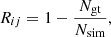 (B.3)
(B.3)
where Rij is the reliability that the given ij pair is a real coincidence, Nsim is the number of simulated LR values, and Ngt is the number of simulated LR values higher than the one observed between the ij pair Ngt = N(LRsimul> LRij). This reliability is then compared with a given threshold. To estimate the threshold, we merged the master catalog with a slave catalog whose coordinates were rigidly shifted in four directions, taking the mean of the resulting matches with varying the threshold. We typically fixed the threshold as the value resulting in a number of spurious coincidences, which is about 10% of the real matches.
As shown in Table B.1, we used the ML method in two matches: steps 9 and 11. In the first (match of the UKIDSS+2MASS+IRAC catalog as master with the WISE catalog as slave), we adopted as representative bands the JHK bands from UKIDSS or 2MASS (choosing for each source the one with the smallest error when they were both available) and the [3.6] band from IRAC. The expected correlated population necessary to calculate q(m) was obtained from a close-neighbors match with  . In step 11 (the match of the optical-infrared catalog as master and the Chandra catalog as slave), we adopted as representative bands the r band from VPHAS+, IPHAS, and Pan-STARRS, the J magnitude from 2MASS or UKIDSS (the one with the smallest error, when they were both available), and the [3.6] band from Spitzer-IRAC. We performed the match in three iterations, updating the expected correlated population in each run and thus the q(m) distributions. In the first iteration it was defined from a close-neighbors match with rmatch = 1″, while in the second and third runs, it was obtained from the ML match performed in the previous iteration. As shown in Table B.2, this strategy did not improve the total number of matches, but it reduced the number of multiple coincidences in the second iteration (the single, double, and multiple columns).
Intermediate steps of the catalog merging process.
Iterations in the OIR-X match.
Each step shown in Table B.1 produced a number of multiple matches. These multiple coincidences were retained in the merged catalog and were then visually inspected when possible. When the merged catalogs provided photometry in similar bands (such as VPHAS+ vs. IPHAS or 2MASS vs. UKIDSS), or when hypotheses can be made a priori on the nature of the merged sources (e.g., the X+OIR sources are expected to be mainly pre-main-sequence stars), it is possible to inspect the multiple coincidences in order to resolve some of them, that is, by separating some of the multiple coincidences that are likely false positives. This iteration was particularly important for the X+OIR match (step 11), as shown in Table B.1. For this match, we also searched for false negatives, that is, nearby OIR sources that are likely real counterparts of unmatched X-ray sources. We performed this search within 5″ from each X-ray source without an OIR counterpart and merged nine OIR sources that from their colors, magnitudes, and proximity to an unmatched X-ray source are likely pre-main-sequence stars.
Appendix C: Extinction coefficients
In this appendix we summarize the extinction coefficients Cλ, where Aλ = CλAV.
Extinction coefficients Cλ.
Appendix D: Color–color and color–magnitude diagrams used to select and classify members
In this appendix we show the diagrams that we used to select stars with a disk and discard contaminants together with the diagrams shown in Fig. 5.
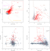 |
Fig. D.1. Infrared diagrams of all sources in the studied field that meet the criteria of good photometry. Figure layout and symbols are the same as in Fig. 5. We show the loci that are expected to be populated by stars with a disk (class II and class I YSOs separated), extragalactic sources, giants with circumstellar dust, unreliable stars with excesses, PAH contaminated sources, and unresolved shock knots. |
 |
Fig. D.2. Pan-STARRS color–magnitude diagrams of all sources in the studied field that meet the criteria of good photometry. Figure layout and symbols are the same as in Fig. 5. We show the loci that are expected to be populated by blue stars with excesses, giants, and galaxies (see the text). |
 |
Fig. D.3. Optical color–color diagrams of all sources in the studied field that meet the criteria of good photometry. Figure layout and symbols are the same as in Fig. 5. We show the loci that are expected to be populated by accreting stars with a disk, stars with unreliable infrared excesses, and possible foreground stars. In the IPHAS r − Hα vs. r − i diagram, the solid black lines are ZAMS at increasing extinction, and the dashed lines mark the locus of A stars, as defined by Drew et al. (2005). The solid green line is a ZAMS with EWHα = −40 Å and EB − V = 1 defined by Barentsen et al. (2011). |
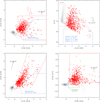 |
Fig. D.4. Infrared diagrams of all sources in the studied field that meet the criteria of good photometry. Figure layout and symbols are the same as in Fig. 5. We show the loci that are expected to be populated by stars with a disk, extragalactic sources, giants with circumstellar dust, and unreliable stars with excesses. |
Appendix E: Details of individual mass and age estimates
Individual parameters of candidate members were estimated by interpolating their positions in selected derreddened color–magnitude diagrams on a grid computed using the 0.5–10 Myr low-metallicity PARSEC isochrones. This method allows estimating the parameters of a large sample of cluster members easily because it only requires the use of good photometry. However, it relies on several assumptions, such as a good knowledge of individual stellar extinctions and the use of stellar models that properly describe the pre-main-sequence phase. Because of the intrinsic uncertainties associated with this technique, results slightly change when different color-magnitude diagrams are adopted, and no strong argument exists that allows us to prefer one diagram over the others a priori. We therefore calculated stellar parameters from seven diagrams listed in the first columns of Table E.1. In all cases, we discarded stars with errors in the involved colors larger than 0.15m and 0.1m in magnitudes. In order to take the photometric errors into account, the interpolation in a given diagram was repeated 300 times for each star, each time drawing the input values of magnitude and color from a normal distribution centered on the nominal values and with a σ equal to the photometric errors. The values of mass and age associated with each star from the given diagram and their errors are thus set as the median value and the standard deviation, respectively, of the resulting distribution of results.
Diagrams used to estimate stellar parameters.
The second and third columns of Table E.1 show the number of members with and without a disk for which the given diagram allowed us to estimate mass and age. These numbers vary because stars may lie outside the isochrone grid in given derreddened diagrams (mainly because of photometric uncertainties, incorrect individual extinction, or blue and red excesses due to disks), which prevents an estimate of their stellar parameters. This is shown in Fig. E.1. In these diagrams, we corrected the low-metallicity PARSEC isochrones with age ranging from 0.5 Myr to 10 Myr for the factor −5.+5 × log(4500), where 4500 pc is the distance to Dolidze 25. Stellar magnitudes and colors were instead dereddened using the individual extinctions found in Sect. 7.2 and adopting the extinction coefficients listed in Appendix C.
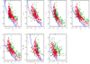 |
Fig. E.1. Derreddened diagrams used to estimate stellar parameters. Low-metallicity PARSEC isochrones (blue lines) were corrected for the distance (4500 pc), while stellar magnitudes and colors were derreddened using the individual extinctions calculated in Sect. 7.2. Stars whose parameters were estimated from the given diagram are marked in red, and the remaining stars are shown in green. |
The resulting mass distributions are shown in Fig. E.2, which shows the resulting distribution changes by adopting different diagrams to estimate stellar parameters. We also compared the observed slopes (calculated by adopting the limits listed in the fifth column of Table E.1) of the mass distribution with that of the normalized Salpeter–Kroupa IMF with α = 2.35 (Kroupa & Weidner 2003). We do not see convincing evidence supporting a deviation of the mass function from the universal law. In order to obtain a unique mass distribution (the one shown in the bottom right panel in Fig. 14), we calculated for each star the average mass value from the individual estimates obtained from the various diagrams in which the star was located inside the isochrones grid. In this distribution, the observed slope matches the normalized Salpeter–Kroupa IMF slope in the mass range 0.8–2 M⊙.
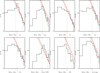 |
Fig. E.2. Mass function distributions of both disk-less and disk-bearing candidate members of Dolidze 25 (the latter considered only if they were inside the ACIS field) obtained from each of the adopted diagrams. The solid black line is obtained from a linear fit in the log–log space on the mass distribution between the two limits marked with the vertical lines. The red line shows the normalized Salpeter–Kroupa IMF with α = 2.35 (Kroupa & Weidner 2003). The range of completeness and the shape of the mass distribution change slightly when individual masses are estimated from different diagrams. The average distribution is obtained by averaging the values obtained from the adopted diagrams for each star. |
Figure E.3 shows the resulting distributions of stellar ages as calculated from each adopted diagram and the resulting average values. None of the distributions obtained from the diagrams show a predominant age, which may be due to a real age spread or to uncertainties associated with the method. The resulting median values are listed in Table E.1. The averaged distribution instead shows a dominant peak at about 1 Myr, with a median age equal to 1.6 Myr, which is the average cluster age adopted in this work.
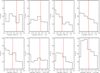 |
Fig. E.3. Distribution of stellar ages of both disk-less and disk-bearing candidate members of Dolidze 25 (the latter considered only if they were inside the ACIS field). The vertical red lines mark the median age values. The average distribution is obtained by averaging the values obtained from the adopted diagrams for each star. |
Appendix F: Catalog of the candidate young stars in Dolidze 25
In this appendix we describe the catalog of the young stars in Dolidze 25 and the surrounding area.
Catalog of the members of Dolidze 25 and Sh2-284.
Appendix G: Disk fractions and ages of the clusters plotted in Fig. 16
Age and disk fraction of the clusters plotted in Fig. 16.
Appendix H: Magnitude distributions
In this section we show the magnitude distributions of the members, control, and ACIS FoV samples, as defined in Sect. 7.4.
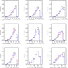 |
Fig. H.1. Magnitude distributions of the members (black), control (blue), and ACIS FoV (red) samples in the given photometric bands. |
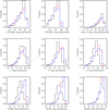 |
Fig. H.1. continued. |
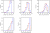 |
Fig. H.1. continued. |
All Tables
All Figures
|
Fig. 1. WISE 12 μm image of the area surrounding Dolidze 25. The red circle marks the area within which we selected stars with a disk, the red box delimits the ACIS-I FoV, the dashed yellow boxes encompass the regions identified and studied by Puga et al. (2009), and the segment in the upper right corner shows the angular extent corresponding to 10 pc at the distance of Dolidze 25. |
| In the text | |
|
Fig. 2. Combined Chandra ACIS-I Images of Dolidze 25. In the left panel, we show an RBG image, with events in the hard energy band marked in red, those in the medium band (1.21–1.99 keV) are plotted in green, and those in the soft band are shown in blue. In the right panel, the white polygons mark the contours of the continuum emission at 8 μm from Spitzer-IRAC, while the red circles mark the position of the validated X-ray sources. |
| In the text | |
|
Fig. 3. Spatial coverage of the sources with good photometry in the catalogs. A central overdensity, corresponding to the approximate location of Dolidze 25, is evident in all the catalogs. |
| In the text | |
|
Fig. 4. Summary flowchart of the procedure adopted to select stars with a disk and pruned candidate contaminants from the list. In each step represented by an oval, the list is pruned of a given class of contaminants. For any selection of contaminants, sources are verified with the corresponding test shown in the boxes. A detailed description of the tests is provided in the text. |
| In the text | |
|
Fig. 5. Subset of the infrared and optical-infrared diagrams of all sources in the studied field that meet the criteria of good photometry (e.g., error in magnitude smaller than 0.1m and in color smaller than 0.15m). The dashed lines show the isochrones for ages 0.5 Myr, 1.5 Myr, 3 Myr, 5 Myr, 8 Myr, and 10 Myr, and with metallicity Z = 0.004 (Delgado et al. 2010) from the PARSEC models, plotted adopting a distance of 4.5 kpc and AV = 2.7m. Red dots mark the selected stars with a disk that we retained in the final list. We also show the loci defined to select stars with a disk and contaminants, delimited by red and green lines. In particular, we show the loci expected to be populated by giants, stars with unreliable excesses, foreground stars, and YSOs with a disk in these diagrams. All diagrams are shown in Appendix D. |
| In the text | |
|
Fig. 6. Spitzer-IRAC image in the [8.0] band of Dolidze 25 and the surrounding Sh2-284 complex. The positions of selected stars with a disk are marked (red circles). The black square delimits the field observed with Chandra. |
| In the text | |
|
Fig. 7. Distribution of the mean photon energy and net counts in the broad energy band for the validated X-ray sources. We show the X-ray sources with and without OIR counterpart separately. |
| In the text | |
|
Fig. 8. Diagrams of all sources in the ACIS FoV that meet the criteria of good photometry (gray points). Figure layout and symbols are the same as in Fig. 5. The large dots are: candidate stars with a disk inside the ACIS FoV (red), candidate young stars without a disk (blue), and X+OIR sources in the foreground or background (yellow). |
| In the text | |
|
Fig. 9. IRAC image in the [8.0] band of the field around Dolidze 25, together with the position of candidate stars with a disk (red), without a disk (yellow) and spectroscopic members (blue). We also indicate the limits of the Chandra ACIS-I field with a square. |
| In the text | |
|
Fig. 10. Minimum spanning tree built on all the members selected inside the ACIS FoV. Members without a disk are marked with blue dots and those with disks with red dots. The yellow stars mark the position of the most massive members. Filled dots mark the position of clustered members, i.e., members that are closer than 34 |
| In the text | |
|
Fig. 11. Pan-STARRS Qrizy vs. i − z diagram of all sources in the studied field with errors in colors smaller than 0.15m. The blue dots mark the observed colors of the candidate members of Dolidze 25, and the yellow dots mark their positions after dereddening their colors. The dashed lines mark the zero-extinction low-metallicity PARSEC isochrones for the pre-main-sequence phase assuming an age of 1.5 Myr. |
| In the text | |
|
Fig. 12. Left: distribution of the individual extinctions of all disk-less members. We separately plot those for sources in the central cluster, northern group, and in the sparse population. The vertical lines mark the median and the 25% and 75% quantiles of each distribution. Right: extinction map in the ACIS field. The red lines mark the emission level at 8.0 μm from IRAC images. The green boxes roughly delimit the central and northern groups. |
| In the text | |
|
Fig. 13. Distribution of individual stellar ages for candidate members within the ACIS field. The vertical lines mark the median value of the distribution. The distribution peaks at about log(age)∼6.0 Myr, with a median age equal to log(age)median = 6.2 Myr. |
| In the text | |
|
Fig. 14. Mass function of the disk-less and disk-bearing candidate members of Dolidze 25 (the latter considered only if inside the ACIS field). The vertical red lines mark the median mass value. The dashed black line is obtained from a linear fit in the log–log space on the mass distribution between 0.8 and 2 M⊙ (values marked with dotted green lines). The red line shows the normalized Salpeter–Kroupa IMF with α = 2.35 (Kroupa & Weidner 2003). |
| In the text | |
|
Fig. 15. Magnitude distribution at [3.6] and zPanSTARRS bands for the control, ACIS FoV, and members samples. |
| In the text | |
|
Fig. 16. Disk fraction vs. age of 58 clusters with ages between 0 and 10 Myr. Nearby clusters, e.g., closer than 1 kpc to the Sun, are marked with large black dots, massive clusters are marked with red dots, and the low-metallicity star-forming regions studied by Yasui et al. (2010) are plotted in green. The average estimate of the disk fraction in Dolidze 25 we obtained by accounting for completeness is marked with stars. |
| In the text | |
|
Fig. 17. Histogram of the FUV (top panel) and EUV (bottom panel) fields for the candidate member. The FUV fluxes are in units of the Habing flux G0, with 1 G0 = 1.6 × 10⁻³ erg cm−2 s−1 (1.7 G0 is equal to the average interstellar UV field in the solar neighborhood in the 912–2000 Å band, Habing 1968). The vast majority of candidate cluster members lies in areas of very low values of the local UV field. |
| In the text | |
|
Fig. B.1. Distribution of total (Ntotal), spurious (Nspurious), and real (Nreal) coincidences in the match of the optical and the infrared catalogs. The distribution of Nspurious becomes comparable to that of Nreal for rmatch between 0 |
| In the text | |
|
Fig. D.1. Infrared diagrams of all sources in the studied field that meet the criteria of good photometry. Figure layout and symbols are the same as in Fig. 5. We show the loci that are expected to be populated by stars with a disk (class II and class I YSOs separated), extragalactic sources, giants with circumstellar dust, unreliable stars with excesses, PAH contaminated sources, and unresolved shock knots. |
| In the text | |
|
Fig. D.2. Pan-STARRS color–magnitude diagrams of all sources in the studied field that meet the criteria of good photometry. Figure layout and symbols are the same as in Fig. 5. We show the loci that are expected to be populated by blue stars with excesses, giants, and galaxies (see the text). |
| In the text | |
|
Fig. D.3. Optical color–color diagrams of all sources in the studied field that meet the criteria of good photometry. Figure layout and symbols are the same as in Fig. 5. We show the loci that are expected to be populated by accreting stars with a disk, stars with unreliable infrared excesses, and possible foreground stars. In the IPHAS r − Hα vs. r − i diagram, the solid black lines are ZAMS at increasing extinction, and the dashed lines mark the locus of A stars, as defined by Drew et al. (2005). The solid green line is a ZAMS with EWHα = −40 Å and EB − V = 1 defined by Barentsen et al. (2011). |
| In the text | |
|
Fig. D.4. Infrared diagrams of all sources in the studied field that meet the criteria of good photometry. Figure layout and symbols are the same as in Fig. 5. We show the loci that are expected to be populated by stars with a disk, extragalactic sources, giants with circumstellar dust, and unreliable stars with excesses. |
| In the text | |
|
Fig. E.1. Derreddened diagrams used to estimate stellar parameters. Low-metallicity PARSEC isochrones (blue lines) were corrected for the distance (4500 pc), while stellar magnitudes and colors were derreddened using the individual extinctions calculated in Sect. 7.2. Stars whose parameters were estimated from the given diagram are marked in red, and the remaining stars are shown in green. |
| In the text | |
|
Fig. E.2. Mass function distributions of both disk-less and disk-bearing candidate members of Dolidze 25 (the latter considered only if they were inside the ACIS field) obtained from each of the adopted diagrams. The solid black line is obtained from a linear fit in the log–log space on the mass distribution between the two limits marked with the vertical lines. The red line shows the normalized Salpeter–Kroupa IMF with α = 2.35 (Kroupa & Weidner 2003). The range of completeness and the shape of the mass distribution change slightly when individual masses are estimated from different diagrams. The average distribution is obtained by averaging the values obtained from the adopted diagrams for each star. |
| In the text | |
|
Fig. E.3. Distribution of stellar ages of both disk-less and disk-bearing candidate members of Dolidze 25 (the latter considered only if they were inside the ACIS field). The vertical red lines mark the median age values. The average distribution is obtained by averaging the values obtained from the adopted diagrams for each star. |
| In the text | |
|
Fig. H.1. Magnitude distributions of the members (black), control (blue), and ACIS FoV (red) samples in the given photometric bands. |
| In the text | |
|
Fig. H.1. continued. |
| In the text | |
|
Fig. H.1. continued. |
| In the text | |
Current usage metrics show cumulative count of Article Views (full-text article views including HTML views, PDF and ePub downloads, according to the available data) and Abstracts Views on Vision4Press platform.
Data correspond to usage on the plateform after 2015. The current usage metrics is available 48-96 hours after online publication and is updated daily on week days.
Initial download of the metrics may take a while.