| Issue |
A&A
Volume 650, June 2021
|
|
|---|---|---|
| Article Number | A122 | |
| Number of page(s) | 12 | |
| Section | Stellar structure and evolution | |
| DOI | https://doi.org/10.1051/0004-6361/202040251 | |
| Published online | 18 June 2021 | |
New analysis of the ρ-class bursts, known as the “heartbeat” of GRS 1915+105: Pulse profile and spectral properties
1
INAF, IASF Palermo, via U. La Malfa 153, 90146 Palermo, Italy
e-mail: This email address is being protected from spambots. You need JavaScript enabled to view it.
2
INFN, Sezione Roma 1, Piazzale A. Moro 2, 00185 Roma, Italy
3
INAF, IAPS, via del Fosso del Cavaliere 100, 00113 Roma, Italy
Received:
28
December
2020
Accepted:
30
March
2021
Abstract
Context. We present the results of a new analysis of three long Rossi-XTE observations of the microquasar GRS 1915+105 in the ρ class, performed in 1997, 1999, and 2000, and characterized by different peak profiles. The first data set, labeled G-1, is dominated by a single peak, while in the third observation (G-3), all bursts show a clearly detectable couple of peaks. The second observation (G-2) shows an intermediate structure with a single peak and an emerging shoulder on the decay side.
Aims. We devised a new procedure to obtain mean burst profiles in every energy channel independently of the recurrence time intervals of the bursts, variable from 45 s to 53 s in the considered observations, with the aim of investigating the different features of peaks and the eventual spectral variations.
Methods. All the bursts were aligned at a common time bin on the decaying portion of the bursts that is stable in simultaneous light curves at different energies. An averaging algorithm was then applied without modifying the statistical properties or scaling the burst lengths. We analyzed the peak amplitude ratios and the dependence of their delays on energy. The spectral distributions were evaluated for the various components: a stable multi-temperature disk plus a power law Comptonization component was used for the baseline emission and temperature differences of peak components were evaluated with the inclusion of an additional blackbody.
Results. In addition to the well-observed double peak (P1 and P2) pattern, we detected a third small peak (P3) in the structured G-3 light curve. This peak, differently from the other two, exhibits a fast rising and a slower exponential decay, with a e-folding time constant of 1.32 s. The blackbody temperatures of P2 and P3 are higher than P1 and the power law spectrum of P3 is the flattest one.
Conclusions. The time and spectral behavior of P3 is interpreted as a signature of a relatively hot plasma outflow from the disk into the corona and its duration is consistent with the crossing timescale of the particles through the corona where electrons radiate.
Key words: binaries: close / stars: black holes / stars: individual: GRS 1915+105 / X-rays: binaries
Retired.
© ESO 2021
1. Introduction
GRS 1915+105 was discovered in 1992 (Castro-Tirado et al. 1992) and later identified with a binary system at a distance of about 12.5 ± 1.5 kpc (Mirabel & Rodríguez 1994) containing a 14.0 ± 4.4 M⊙ black hole (Harlaftis & Greiner 2004). Reid et al. (2014), using the Very Long Baseline Array (VLBA), measured the trigonometric parallax of the radio source associated with GRS 1915+105 and derived a distance of 8.6 kpc. This allowed for a new estimate of the black hole mass of 12.4 ± 2.0 M⊙ that is lower but still compatible with the prior value.
The X-ray emission of GRS 1915+165 is characterized by a complex variability that alternates between steady, noisy emission and regular bursts. A first classification of the observed time profiles into twelve classes was established by Belloni et al. (2000) and later extended with the detection of new patterns (e.g., Klein-Wolt et al. 2002; Hannikainen et al. 2005). This classification is now largely adopted in the literature and we will refer to it in the present paper. One of the most interesting variability classes is the so-called ρ class in which long series of nearly regular bursts are observed with a variable recurrence time Trec ranging from about 40 s to about 90 s. This bursting behavior was discovered by Taam et al. (1997), who recognized the pattern expected from a thermal-viscous instability in accretion disks presented a few years before in Taam & Lin (1984). A similar variability pattern, but more irregular and with shorter Trec, was also observed in the source IGR J17091+3624 (Altamirano et al. 2011) and, more recently, Bagnoli & in’t Zand (2015) reported the discovery of a behavior similar to that of the ρ class in the X-ray binary MXB 1730-335 (Rapid Burster) with a quite long recurrence time of about seven minutes.
The structure of ρ-class bursts is complex: in many cases it presents a double peak, and, on other occasions, it appears with a single or, more rarely, a multiple feature. The double peak structure, already reported in the discovering paper by Taam et al. (1997), was investigated and discussed by Neilsen et al. (2011); Neilsen et al. (2012). In particular, Neilsen et al. (2012) performed a time-resolved spectral analysis for single- and double-peaked bursts and found that these two patterns essentially exhibit a similar X-ray spectral evolution that is related to a thermal-viscous instability.
Several properties of the ρ class of GRS 1915+105 using data series obtained in long duration observations of this source with BeppoSAX in October 2000 have been investigated (Massaro et al. 2010; Mineo et al. 2012; Massa et al. 2013; Maselli et al. 2018). Massaro et al. (2010) introduced a further classification of the ρ bursts, from p1 to p4, where the digit is the number of narrow peaks that can be distinguished in each pulse profile. In that paper, striking relations between certain relevant parameters, such as the correlation between the mean recurrence time and the flux level, were obtained. Later, Maselli et al. (2018) found a power law dependence of the pulse width on energy.
In this paper, we analyze three specific Rossi-XTE observations of GRS 1915+105 in ρ class (see Table 1) that were already considered by several authors in their studies of the properties of this mode. Neilsen et al. (2011) published their analysis on one of these observations (G-3 in Table 1) and, subsequently, reconsidered the same data and compared the results with those of a second pointing (G-2 in Table 1), and then performed a time-resolved spectral analysis (Neilsen et al. 2012). These two observations, and particularly their timing properties and quasi-periodic oscillations, were investigated also by Yan et al. (2017); Yan et al. (2018). Previous analyses of the third observation (G-1 in Table 1) were performed by Vilhu & Nevalainen (1998), who reported annular structures in the hardness ratio, and by Titarchuk & Seifina (2009), who included the same observation in a rich sample of pointings focusing the analysis on the mean spectral properties. Maselli et al. (2018) also considered these data for the analysis of the dependence of the burst width on the energy. The study presented in this paper describes the procedures to identify a mean burst profile and compares the different structures found in the peaks of the three observations. Moreover, for the first time, we identify and analyze a third peak detected in the G-3 light curve.
Rossi-XTE observations of GRS 1915+105 considered in the present analysis.
Data and selection procedures are illustrated in Sect. 2 and the method for evaluating mean burst profiles and the structure analysis are described in Sect. 3. Results relative to the structure of burst with triple peaks are presented in Sect. 4. The hard-X delay with respect to energy is presented in Sect. 5 and the spectral analysis is presented in Sect. 6. The comparison with previous results and implications for the physical modeling of the source are discussed in Sect. 7.
2. Observations and data analysis
2.1. Observations
Rossi-XTE (Jahoda et al. 1996) observed GRS 1915+105 on a number of occasions. In this paper, we considered only three long-enough pointings, hereafter, labeled G-1, G-2, and G-3, in which the source exhibited sequences of bursts with rather similar Trec. The log of the considered observations is given in Table 1. We created filters and good time interval (GTI) files applying all standard criteria. The level of the background for the light curves of each of the three pointings was evaluated with standard procedures1. PCA light curves in 15 energy bands in the range from keV to about 13.0 keV with a time bin of 0.125 s were produced using data in binned-mode with 16 energy channels and 8 ms time resolution. For our analyses, the data were rebinned at 0.5 s to limit the statistical noise.
The original data series were divided in intervals of ∼2500 s because of the source occultation during the satellite’s orbit. We removed these gaps, obtaining continuous series, to simplify the analysis: the last peak of a segment was superposed to the first peak of the subsequent one and both series were cut at the bins with common minimum amplitudes and these segments were joined together without inserting interpolations or bridging the data. The exposures reported in Table 1 are the lengths of the final series and the number of useful bursts is the one we obtained after this procedure. No background subtraction was applied in the light curve accumulation because it was found to be negligible compared to the source count rate, even in the portions of the bursts with the lowest count rates at the highest energies: ∼2 ct s−1 against ∼100 ct s−1; much lower, therefore, than the observed fluctuations.
2.2. Data analysis
In the present analysis, we face with the problem of obtaining the mean burst profiles. It has been reported in several papers that recurrence time of burst is not periodic and that large differences are found between the duration of two consecutive bursts. This is clearly apparent from Fig. 1, where three segments of nine bursts of each data series are represented. We note that the time distance between the maxima of subsequent peaks is variable and that in some cases, it can reach a few seconds. The bursts of the three pointings that we considered appear similar but there are some interesting different structures that emerge when many energies are taken into account and an accurate averaging of data is performed. In particular, practically all bursts of the G-3 series are of p2 type, showing a clearly detectable second peak whose relative intensity increases with energy up to overcome the height of the preceding peak at around 9 keV, as discussed in detail in Sect. 4. This point for the G-3 series is accurately investigated by Neilsen et al. (2011).
 |
Fig. 1. Segments of the observations at the energy of 4.1 keV with a time bin size of 0.5 s: G-1 observation is shown in the left panel, G-2 in the central panel, and G-3 in the right panel. The vertical red lines mark the position of the maxima to better illustrate the variations in the duration of the bursts. We note that the time separation between vertical lines is not constant and that the peaks present different shapes in the three observations. |
Given that the bursting is not a strictly periodic phenomenon, we prefer to use the nomenclature of recurrence time, Trec, instead of period. To understand how Trec may be stable in each data series we calculated the Fourier periodograms, given in Fig. 2, and derived the period Tp corresponding to the highest power, which is a good estimate of ⟨Trec⟩. The G-1 series is dominated by a single narrow feature at Tp = 48.17 s, some other peaks are present in the range from about 40 s to about 60 s, but none of them have a power comparable to the main one. A similar situation was found for the G-2 series, with a dominant narrow feature at Tp = 45.02 s; another single peak is found at 48.58 s, while two other close features are between 43.5 and 44.5 s, with a period resolution of 0.1 s. The periodogram of the G-3 series is remarkably different because, together with the peak emerging at Tp = 48.85 s, there is a close group of three other peaks, which are well separated by the previous one, at 52.40 s, 52.82 s, and 53.70 s. This peculiar double structure originates from a significant change of the mean recurrence time in the course of the pointing, which includes four orbital runs longer than 6000 s. We divided this series into three shorter segments indicated by the roman numbers I, II, III, as reported in Table 1, and computed their periodograms, resulting in a single dominant feature, whose corresponding Tp values are also given in Table 1. Thus, the mean recurrence time of bursts had a systematic increase by about 7 s (corresponding to about 14%) from the beginning to the end of the G-3 observation. The most relevant consequence of these changes is that the construction of a mean burst profile is difficult because no absolute phase can be assigned to individual photons and any adaptive algorithm can introduce biases in the analysis. The new approach we followed to overtake this problem is described in detail in the following subsection. We then identified in the mean burst profiles some time intervals to be applied to individual bursts in order to select events for deriving the photon energy spectral distributions. The new method does not affect the statistical deviations with respect to the mean profile and it allows us to investigate modifications that are due either to the turbulent gas properties or to the unstable process itself.
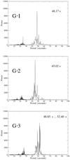 |
Fig. 2. Fourier periodogram of the entire observations at the energy of 4.1 keV with a time bin size of 0.5 s. The plot in the top panel is relative to G-1, that in the central panel to G-2 and the one in the bottom panel to G-3. The period values corresponding to the peaks are reported here. |
2.3. Best-folding problem and mean burst profiles
The changes of Trec make it difficult to obtain reliable mean burst profiles at different energies necessary for a structural and statistical analyses. As we showed in a previous work (Massaro et al. 2010), these variations are mainly due to changes in the duration of the slow leading trail (SLT, i.e., the initial segment of the burst to P1), while the peak width, but not the height, remains more stable. Any technique based on the scaling of individual burst duration to a unique period, as the one corresponding to the highest peak in the periodogram or to any other fixed value would modify the relative phase of features and its superposition would smear out or broaden any structure in the resulting mean profile (see, for instance Neilsen et al. 2012; Yan et al. 2018).
We adopted an alternative approach by aligning all bursts at a feature that appears stable in simultaneous light curves at different energies. As example, we display some bursts in Fig. 3, where we report the data series at three different energies for all the pointings. Their count rates are normalized, as described in the Appendix A. In the G-2 data, the occurrence of the peak maximum appears more synchronous than in other two series. The G-1 and G-3 series, in fact, present more structured profiles and the time position of the main peak maxima for increasing energy is delayed with differences up to about 2 s and occasionally even higher (this issue will be discussed in Sect. 7). A more stable feature, particularly at lower energies, appears in the decaying portion of the bursts, which are generally synchronous within one time bin. We decided, therefore, to use this final portion of the decay to align the bursts of G-1 and G-3 at their times, independently of the actual duration of the SLT, and thus without stretching or compressing the burst duration. Once all the profiles were aligned, we then computed the mean of the counts in each time bin and thus obtained the mean pulse profiles for all the energy channels of the three observations. For the sake of consistency, we also analyzed the G-2 data series using the same method. A detailed description of the algorithm used for computing the mean profiles is given in Appendix A.
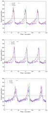 |
Fig. 3. Short segments of the G-1 (top panel), G-2 (central panel) and G-3 (bottom panel) observations in different energy channels showing three consecutive bursts with a time binning of 0.5 s. The count rate has been scaled to be in the range 200–600 counts per bin. The horizontal lines correspond to the level of 350 counts per bin used for the selection of the folding phase marked with the vertical green lines. |
3. Mean burst profiles
The resulting mean profiles of the considered observations at three different energies are presented in Fig. 4. To simplify the comparison of the main features, we subtracted the offset level and then normalized to unity the height of the first peak that is the dominant one at low energies, whereas the second peak was not always clearly detected.
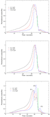 |
Fig. 4. Normalized mean pulse profiles in three energy channels. Individual bursts are aligned at the point of the decay portion marked by the green vertical lines. The time binning is 0.5 s. Top panel: mean profiles for the G-1 data. Central panel: mean profiles for the G-2 data. Bottom panel: mean profiles for the G-3 data. The three peaks, P1, P2, and P3, are indicated with labels. |
One of the major achievements of the adopted folding method is that the substructures of the burst are well resolved. Our results confirm the previous finding of the single peak structure of G-2 (central panel in Fig. 4), while the double structure of G-3 appears in the two well-separated main peaks, indicated as P1 and P2 in the bottom panel of Fig. 4. The case of G-1 (top panel in Fig. 4) appears intermediate between the two other series: at low energies, the second peak, if present, appears as a mild shoulder and at high energies the maximum of the burst profile is delayed in correspondence with the shoulder.
A new and interesting feature present in the G-3 mean profiles and not clearly reported in previous works of the same data, is a small but significant peak which follows P2 by 4.5 s and hereafter indicated as P3 (see bottom panel of Fig. 4). The spectral energy distribution of this peak is more difficult than for both P1 and P2; as discussed in Sect. 7, its amplitude ratio to P1 increases by a factor of about 3 from 4.1 keV to 13.2 keV, whereas P2 almost doubles its value. The statistical analysis of the significance of this feature and its spectral properties are discussed in the next section.
The amplitudes of the peaks in the G-3 mean profiles are clearly dependent upon energy, as directly visible in Fig. 4. To quantify these differences, we computed the peak amplitude ratios between P2 and P3 with P1 that are nearly independent of the instrumental energy response function. We first subtracted the constant base line value and, considering that the peaks are partially overlapped, we then computed the residual content of the three bins including the maxima as shown in the two plots in Fig. 5. The resulting peak amplitude ratios vs. energy are reported in Fig. 6. It is very interesting to note that these energy dependences have a very tight linear correlation – the linear correlation coefficient r = 0.999 for P2/P1 and r = 0.981 for P3/P1. The P2/P1 ratio increases by a factor of 2.1 in the entire energy range while the change of P3/P1 is 3.8, indicating that P3 is the hardest feature. These very high correlations should be explained by means of different energy distributions.
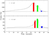 |
Fig. 5. Two mean profiles at different energies of the G-3 data set. The three bins that are indicated as wide, colored areas are the ones used for computing the peak amplitudes ratios. |
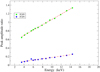 |
Fig. 6. Peak amplitude ratios of P2 and P3 to P1 vs. photon energy. Dashed and dash-dotted lines are the linear best fit. |
4. The triple peak structure of G-3 bursts
The existence of a third peak, P3, clearly identified in the G-3 observation, had not emerged in previous analyses based on the same data set, likely due to the difference in adopted methods. Other mean burst profiles, as those of Neilsen et al. (2011); Neilsen et al. (2012) or Yan et al. (2017); Yan et al. (2018), do not show any resolved feature as our P3 does. In particular, Neilsen et al. (2011) defined the “hard X-ray tail” as a phase interval of ∼5–10 s after the end of the second peak in the [9.0–30.0] keV mean burst profile, where the hardness ratio (HR2) reaches the highest value, even if a resolved peak is not present. Our method of burst folding gives a well-defined time profile of P3 that is useful for investigating the time evolution of this feature at different energies. A detail of the P3 feature is given in the upper panel of Fig. 7, where the statistical errors of the mean counts per bin are also reported. Here, we used only the G-3III data set in the energy band [9.1–15.1] keV, where this feature is more prominent, and the lower peak width reduces possible smearing out of its profile due to the changes of Trec. The statistical significance is indeed very high: if we consider only the four bins with the highest count rate, the excess with respect to the constant level defined by the minimum between P2 and P3 (the horizontal line in the top panel of Fig. 7) is about 95 standard deviations. This is because the Poissonian error of the mean count rate is divided by the square root of the burst number (122) considered in the averaging procedure. We note that the shape of P3 differs from those of the two other peaks: it exhibits, in fact, a fast rising and a much slower decay. More details on its structure will be given in the following paragraphs.
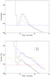 |
Fig. 7. Mean burst profile of the structure of the P3 feature in the three observations. The upper panel is relative to G-3 data in the energy range [9.1–15.1] keV. The blue line defines the constant level used for computing the excess and statistical errors in each bin (0.5 s width) are reported, the dashed line is the linear extrapolation of the last two bins along the P3 profile. In the lower panel profiles relative to G-1 and G-2 are shown, with the energy ranges corresponding to the five highest energy channels: [8.6–13.0] and [7.8–12.9] keV, respectively. |
We searched for a similar feature in the mean profiles of the other two data sets. We applied the same method of adding the mean profiles in the five energy channels at the highest energies where this feature is expected to be more significant than at lower energies. The resulting accumulated histograms are shown in the lower panel of Fig. 7. It is apparent that here the relevance of P3 is not so clear as in the G-3 data set; however, we cannot exclude its existence because an excess appears in the final segment of the peak tail. It is also interesting to see that the maximum of this feature appears aligned with the linear extrapolation of the last bins in these two profiles (lower panel in Fig. 7), while in the G-3III series the bin content around the maximum are well above the best fit line. A first consideration is that P3 appears related to the strength of P2: they are, in fact, more apparent in the G-3 data set than in the other two.
Figure 4 shows that the amplitude of this new feature is higher in the high energy channels than in the low energy ones. This is an indication that the spectrum of P3 is harder than that of the two other peaks, as confirmed by the spectral analysis (see Sect. 6).
An interesting characteristic displayed by P3 is the way its profile varies from that of P1, as well as the stability of its shape. In Fig. 8, we plot the mean profiles of the G-3III series in the five energy channels from 6.8 to 14.4 keV following the subtraction of the minimum base line level and the normalization of the maximum to 100: these shapes are remarkably similar and the dots in each bin are their average values. Their evolution follows a typical Fast Rising Exponential Decay (FRED) behaviour, using a terminology adopted for Gamma-Ray Bursts (Fishman & Meegan 1995; Fenimore et al. 1996) and also applied to X-ray novae (Chen et al. 1997). We use a log scale on the ordinate axis to show the exponential tail and tried to represent the entire profile by means of a Gamma distribution that is a combination of a power law with an exponential decrease:
 (1)
(1)
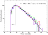 |
Fig. 8. Comparison of five mean profiles of P3 from the G-3III observation in the energy channels in the band [6.8–14.4] keV, normalized in amplitude assuming the maxima equal to 100. Black filled circles are the mean values and the error is the dispersion of these values and the dashed line is the plot of the given best fit formula. The black vertical line indicates the position of the maximum computed applying the same best fit law. |
with α > 0. The maximum of this function is at the time tM = ατ + t0 and the peak flux is FM = F0(ατ/e)α. A simple best fit, with a fixed t0 = 38.0 s gives for the two other parameters α = 1.2 and τ = 1.32 s independent of energy. The resulting curve is also plotted in Fig. 8 and the agreement with data is fully satisfactory.
5. Hard-X delay
One of the more interesting characteristics of the ρ class bursts is that the peak times at high energies are progressively delayed with respect to the low energies. This effect, named the hard-X delay (HXD), was previously reported by Taam et al. (1997) and Paul et al. (1998) and analyzed by Massa et al. (2013) using BeppoSAX data. These authors developed a method for evaluating this delay from the comparison of the [1.7–3.4] keV light curves with those in the [6.8–10.2] keV range and found that it is increasing with the recurrence time of the bursts and also with the count rate of the baseline level (BL) over which the bursts are superimposed.
Mean burst profiles, as computed here, provide further evidence for the HXD phenomenon and allow us to investigate how it evolves at different energies. The HXD is clearly detectable also in the data of all the three observations, and particularly of the G-3 set. The normalized mean profiles in several energy channels in Fig. 4 show their evolution with energy. We report in Fig. 9 a few details, including the peaks of the G-1 (upper panel) and G-3III (lower panel) sets. As described in the Appendix, the data were scaled by assigning the values of 600 to the mean value of peak maxima and of 200 to the mean value of burst minima, respectively. In both observations, it is apparent that the maximum of P1 is progressively delayed and, at the highest energy, this delay is 2.0 or 2.5 s, whereas at the half-width height (that corresponds to the level of 400 in the two panels), the delay is of 5 s and reaching 6 s in the G-3III data. There is, therefore, a correlation between the shape of the SLT and the width of the “Pulse”, as reported by Maselli et al. (2018). In the lower panel of Fig. 9, we can see that a similar trend does not occur for the other peaks: the valley between P1 and P2 at about 40 s (marked with a green vertical line) and the maximum of P2 at about 42 s (marked with a gray vertical line) do not vary with energy. The same effect cannot be seen in the G-1 data because, as has already been noted, the P2 feature is closely blended with P1 without any minimum between them. The variations of the peak position observed in G-2 data are not larger than ∼1 s, similar to those found for P2 in G-3 light curves.
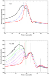 |
Fig. 9. Segments of normalized mean profiles. In the upper panel three normalized mean profiles of the G-1 bursts at the energies of 2.5 (thick black line), 7.5 (thin blue line), and 12.5 keV (red thick line) are shown. Short vertical lines mark the maxima of P1 and the long vertical line marks the shoulder. The lower panel presents segments of normalized mean profiles of the G-3III bursts in some energy channels from the lowest (3.5 keV, thick black line) to the highest one (14.4 keV, red thick line). Long vertical lines mark the maxima of P2 and the minima in valley between P1 and P2; short vertical lines mark the maxima of P1 at the extreme energies. We note the constant time distance between the minimum between P1 and P2, the maxima of P2 and P3, while the time of the P1 maximum shifts by 2.5 s. |
In Fig. 10, we report the time separation between the maxima of P1 and P2 for the G-3 series as function of the photon energy and the resulting HXD computed by subtracting the values of the separations from the one at the lowest energy. The accuracy of each value is equal to the adopted time bin width (0.5 s) and, therefore, we computed also the linear best fits, which could be representative of the actual change of these quantities with energy. This amount of HXD is less than the one reported in Massa et al. (2013), which, for bursts having a similar recurrence time, is equal to about 4 s. This difference can be due to the different methods adopted in these analyses since in Massa et al. (2013) it is considered the times of the highest values in the energy data that occur after the maxima in the light curves.
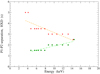 |
Fig. 10. Time separation between the maxima of P2 and P1 (red filled circles) and the HXD (dark green filled diamond) of the G-3 data set. The dashed and the dot-dashed lines are the linear best fits to these sets. |
Time shifts are not found between P2 and P3: the distances between their two maxima correspond to an average value of 4.5 ± 0.2 s, where the error is the rms of the values in all energy channels. If a non-statistical uncertainty for the peak maximum positions equal to the half bin width (0.25 s) is taken into account, the total error increases to 0.3.
This result appears clearly in the lower panel in Fig. 9, where a detail of some pulse profiles are shown at different energies across the entire range. The only measured delay is therefore between P1 and the other features, which maintain stable their mutual separation. We note also that a similar separation might exist in the G-1 light curves, but in this case, the position of the P3 maximum is quite uncertain because of its shallow profile.
It is also possible to verify the magnitude of the change of the P1 height with respect to P2: in the G-3III (Fig. 9, lower panel), the former feature decreases by a factor of ∼2 from the energy of 3.5 keV to 14.4 keV. We also note in Fig. 4 the change of the SLT increasing rate, which, in the highest energy channels, exhibits a plateau having a duration of 10 or 12 s before the sharp fast rise to the peak maximum. Similar changes are likely present in the G-1 data set, but an estimate of the amplitude is not possible without a modeling of the two peaks, which remains largely arbitrary. In any case we can see that at the lowest energy, P2 appears as a shoulder on the decay side of the peak, while at the highest energy, it might reach a comparable height. These changes are clearly related to the different spectral distributions of the two feature, as it will be discussed in detail in Sect. 6.
6. Spectral analysis
The burst’s multicomponent structure, described in the previous sections, and its energy evolution imply that the energy spectra of individual components are different. The general approach to spectral modeling of bursts that is usually adopted in other analyses is based on a standard thermal emission model from a thin accretion disk in stable equilibrium. The ρ class bursting cycle is originated by a non-linear instability, which can modify the disk configuration and the superficial temperature distribution. One issue is that the minimum level of bursts is remarkably stable and the initial development of the burst is rather slow; it is, therefore, possible that these minima correspond to an equilibrium state that it is perturbed when brightness starts to increase.
Our first step was to fit a disk model to data in an interval of a few seconds around the minimum of each burst, corresponding to what we named the BL level. We considered the two data series of G-2 and G-3III, the former one because its bursts have the simplest structure, with a single peak, and the latter data for the possibility of separating the peak maxima, while G-1 exhibit an intermediate state with the two main peaks blended together. The data of BL were accumulated in a single spectrum having 15 energy bins. We used the Zimmerman et al. (2005, EZDISKBB in XSPEC) model that assumes Newtonian accretion disk with zero torque at the inner boundary and a temperature profile that does not diverge for small inner radii. The main model parameters are the inner radius Rin and the temperature Td of the disk. We added to this model a low energy absorber and a high energy tail to represent a possible Comptonization component. Our previous analysis showed that the spectral emission of this source requires a hybrid Comptonization model (Mineo et al. 2012, 2017); however, the small PCA energy range we fitted (3.3–15 keV) does not allow for such a complex model. We then adopted the simple scattering component described by the XSPEC model SIMPL (Steiner et al. 2009) that takes any seed spectrum (the hot multi-temperature disk in our case) and scatters a fraction fsc of the photons into a power law with spectral index Γ. The low energy absorption was introduced with the XSPEC model TBABS assuming element abundance from Wilms et al. (2000) and cross-sections from Verner et al. (1996). In summary, our fitting XSPEC model for the BL level spectra was TBABS*SIMPL*EZDISKBB. Finally, we assumed the source distance of 8.6 kpc (Reid et al. 2014), and we did not include Fe emission line around the energy of 6.4 keV in the best fit calculations because, given the energy resolution of PCA units, no significant evidence for this feature was found. The same model was already used by Neilsen et al. (2011), who considered this line and also a high energy exponential cut-off for the power law whose e-folding energy in the BL interval resulted ∼50 keV. This introduces a decrease in the flux of about 10% at 5 keV that increases to 23% at 13 keV. As we discuss further on in this paper, this model is not well suited for the P3 data and a different solution is necessary, which we propose here.
To extract spectra relative to the peaks, we defined for each burst in the G-3III data set, three time intervals of a few seconds in correspondence to the peak maxima. These intervals are broader than those shown in Fig. 5, with the goal of reaching an adequate signal-to-noise ratio. In the fitting procedure, a systematic of 0.8% was considered, as suggested in the Rossi-XTE user manual2, and errors on the best fit parameters correspond to a 90% confidence level.
6.1. Best-fit spectra of BL in the G-2 and G-3III observations
Photons of these two observations were accumulated in BL intervals around the minima, having a duration from 6 to 9 s, depending on the individual burst profiles. The spectral model described above gives acceptable best fits to the BL for both data sets. The resulting parameter values and reduced χ2 are reported in Table 2. There is a good agreement between the results of the two observations implying that the physical conditions and the size of the disk, when the source is in the ρ class, are rather stable and not affected by the pattern of bursts. These spectral results agree with the ones published by Mineo et al. (2012), who considered a ten-day BeppoSAX observation performed in October 2000, where the equivalent Hydrogen column was in the range (4.3–5.3) × 1022 cm−2. Also, the values of Rin are coherently ∼50% lower than those derived with the higher distance of 12.5 kpc assumed in Mineo et al. (2012).
Spectral best-fit parameter values for the baseline level (BL) data of the G-2 and G-3III spectra with the model TBABS*SIMPL*EZDISKBB.
We also computed the best fits with the model TBABS*SIMPL*DISKBB, which has the same parameters, for a better comparison with the literature analyses and for the purpose of better understanding how the choice of the emission model affects the parameter values. The results are fully compatible with those of Table 2, with the only marginal exception of Rin, which turns out to be 14.5 km for G-2 and 16.6
 km for G-3III (as in Table 2, the errors correspond to a confidence level of 90%). These values are lower than those resulting from the EZDISKBB model by a factor of about 1.6. These values of Rin are compatible within one standard deviation with the Schwarzschild radius RS = 2GM/c2, which for a black hole of 10 M⊙ is 30 km, but not with the radius of the last stable orbit at 3RS. This result suggests a rapidly rotating black hole, which is in agreement with previous findings (Middleton et al. 2006; Mineo et al. 2012; Neilsen et al. 2012). The comparison with the Neilsen et al. (2011) results is presented in the next section.
6.2. Spectral analysis of the peaks
A specific phase-resolved spectral analysis was performed for the single peak of G-2 and on the three peaks of the mean profile of G-3III data, selecting count rates in several time intervals. For the single peak bursts of G-2 data, we selected events in a time interval having a duration from 3 to 6 s centered at the maximum depending on the burst width. On the other hand, in each burst of the 15-energies light curves of the G-3III pointing, the data were extracted in three intervals around the maxima of P1, P2, and P3 with the same criteria as for the G-2 spectra; in particular, the intervals have durations of 5.5–7.0 s around P1 and 3–4 s for P2 and P3, without any overlap among them.
The same model adopted for the BL data gives acceptable spectral fits, but, in the case of P3, which is located at a small height above the BL level, some parameters were highly affected by the large BL contribution. The BL spectral dominance in the phase interval of P3 can be the reason for the temperature estimates very close to the SLT that have been reported by Neilsen et al. (2011), while the Hard-X Tail and our results on the peak amplitude ratios, without the BL contribution (see Sect. 3), show that it must have a hotter spectrum.
We intended to evaluate the temperature differences between the peaks’ emission with respect to that of the BL and, therefore, we considered adding another component. We tried for this component (i) a second multi-temperature disk, (ii) a Band-like spectrum, and (iii) a blackbody (BB). Only the last model gave always acceptable fits; the fitting procedure with two multi-temperature disks did not converge for the P2 spectrum, and the band-like spectrum always produced reduced χ2 > 3. The resulting parameters for the only acceptable model (TBABS*SIMPL*(EZDISKBB+BBODY)) are given in Table 3. In the fitting of the peak spectra, we fixed the disk parameters to those of the BL spectrum, while the parameters of the blackbody and of the empirical Comptonization (the power law index Γ and the scattered fraction fsc) were left free to vary. For the P2 spectrum, however, because it was not possible to obtain reliable errors of the best fitting values, we fixed the fsc to the P1 value. Initially, we left the value of NH free to vary and found that all best fit values were compatible within the errors with the BL one, therefore we fixed that value in the spectral analysis.
Results of the phase resolved spectral analysis of the G-2 and G-3III spectra with the model TBABS*SIMPL*(EZDISKBB+BBODY).
In Fig. 11, we plotted the evolution of the best fit values of kT and Γ along the profile. It is interesting to note the clear anti-correlation between these values; however, we have to take into account that a lower value of Γ corresponds to a harder spectrum. Considering that the fraction of scattered photons is stable, this correlation implies that the temperature increase of the peak components is related to an increase at high energy detected as a flattening of the power law. In Fig. 12, we show the two spectral components of the three peaks present in the G-3III data and their sum (solid black line) plotted on the deconvolved data, which resulted in a fully satisfactory agreement. We can see the temperature evolution of the blackbody component produced by the change of the peak energy.
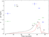 |
Fig. 11. Best-fit values of kT (dark green filled circles) and Γ (blue filled triangles) of the BL and peak spectral best fits of the G-3III observation. Reported errors correspond to 1 standard deviation. Mean pulse profile at the energies of 4.1 (black) and 13.2 (red) keV to show the time correspondences are plotted. |
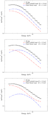 |
Fig. 12. Best-fit spectral components of the three peaks of the G-3III data set, including the low energy absorption and the Comptonization to a power law. We note the increasing blackbody temperature from P1 to P3. Statistical uncertainties of the data are two orders of magnitude lower the values and are not visible in these plots. Top panel: black diamonds and deconvolved data for P1 and the black solid line is the total flux resulting from the sum of the EZDISKBB (red) and BBODY (blue) lines; central panel: same model for P2; bottom panel: same model for P3; we note the high energy flattening due to the Compton scattered photons. |
The present estimate of kT for the blackbody component at the P2 maximum, which measures the temperature difference with respect to the BL value, is lower than the one given by Neilsen et al. (2011, see their Model 1), which is higher than 2 keV. We have to take into account that the multi-temperature model by Zimmerman et al. (2005) peaks around kT, while the peak energy of the BB component is at 2.8 kT and, therefore, our temperature estimates turned out to be lower.
The comparison of these spectral results with those published by Neilsen et al. (2011) is not straightforward because of the differences in the widths of the time and energy intervals we adopted to accumulate the spectra. In fact, our time intervals are larger than the those in Neilsen et al. (2011), and our best-fit values should be compared with the averages in the correspondent intervals. Moreover, our analysis is performed in a smaller energy range that does not require any high energy cut-off (which typically introduces a strong negative correlation between the disk kT and the power law index Γ). Taking into account these considerations, we tested the consistency of our analysis by fitting the spectra with the model TBABS*SIMPL*EZDISKBB and computed the range of variability of each parameter obtained by Neilsen et al. (2011) in the time intervals corresponding to our spectra and then applied them to limit the best fitting. We found χ2 acceptable for all intervals, except for P3, where the high reduced χ2 = 3.2 was obtained. However, the best-fit values for the BL in Table 2 were obtained by relaxing this constraint in the parameter ranges. Thus, we found a better solution (χ2 = 0.98 instead of 1.3), with values marginally compatible with those found by Neilsen et al. (2011).
7. Summary and discussion
We performed the analysis of three RXTE observations of GRS 1915+105 in the bursting ρ class, applying a new approach that is markedly different from methods used in earlier analyses (e.g., Neilsen et al. 2011, 2012; Yan et al. 2017, 2018) and obtaining a number of notable findings. Our first step was the development of a folding tool for computing a mean burst profile without the assumption of phase values related to a unique mean Trec, because it varied from a burst to the following one and the burst shape did not follow a similar scaling. On the basis of the comparison of simultaneous light curves at different energies, we searched for a common feature at which individual bursts could be aligned. Then we selected a time bin in the decay trail of the main peak. In the cases of the G-1 and G-3 series, this choice gives quite different results with respect to whether we adopted the burst maxima or the minima, while for G-2, which has the simplest structure, the alignment at the peak maxima was satisfactory as well. A further advantage of this method is that it does not affect the count rate fluctuations in every time bin, with a few exceptions in the short initial and final segments, where possible superposition may occur (see Appendix A). Thus, this method can be used to investigate the statistical properties of the large changes exhibited by GRS 1915+105, which will be presented and analayzed in a forthcoming paper.
Once we obtained the mean burst profiles in every energy channel, we noticed that the G-3 series presents, in addition to the main double peaked structure, a third and lower but well-resolved peak (named P3), whose amplitude relative to the other peaks is increasing with energy. This peak is not so clearly apparent in the two other observations, although our analysis shows that it might be present but with a much lower amplitude.
We successfully modeled the FRED time evolution of this peak by means of the formula of Eq. (1), that can be considered as a very simple approximation for describing the development and decay of a electron-photon shower (see, e.g., Rossi 1952; Schiel & Ralston 2007). It is interesting to note that the profile of P3 is remarkably different from those of the other peaks; furthermore, the fact that it is stable with regard to the energy suggests that the evolution of this feature is not directly ruled by the disk instability producing the other structures. Neilsen et al. (2011) reported the occurrence an unstructured “hard X-ray tail” on the basis of the hardness ratio plot and proposed that it can be the signature of a relatively hot plasma outflow from the disk and injected (or evaporated) into the corona and emitting a short radiation flare. The possibility of a plasma outflow from magnetized accretion disks was early investigated by Blandford & Payne (1982) and was developed by Janiuk et al. (2002), who showed that an outflow can be a damping mechanism of the non-linear bursting, as those of the ρ class. Our results are not in conflict with this interpretation. The finding that the time evolution of P3 is energy-independent could be interpreted as the decay timescale of about 1.3 s representing the ejection or the crossing timescale of the particles through the corona where electrons can radiate via bremsstrahlung. It would be useful to extend the same analysis to other observations in the ρ state to search for the cases where this third peak is fully detectable, as in the case of G-3III, and to check whether its parameters are correlated with some structural or spectral properties of the other main peaks; in particular, the occurrence of a double peak pattern. The search for physical properties related to a high P3 amplitude will be useful for understanding the process that leads to this feature.
The physical interpretation of the best-fit values of Rin as the effective inner radius of the disk (∼50 km, as we have shown for the BL component in Table 2) is compatible with a rotating blackbody, as has already been reported in a number of papers (Middleton et al. 2006; Mineo et al. 2012; Neilsen et al. 2012).
An issue that still is not fully understood is the interpretation of the main double peak structure, as the one that is clearly apparent in G-3, but not always present as in the case of the G-2 series, or partially superposed as in the G-1 data, where the second peak appears as a shoulder in the decaying trail.
In each G-3 burst, the two peaks are clearly separated and have a slightly variable distance. In the case of the G-1 observation, the second peak is partially blended with the first one and appears as a shoulder on the decay side: the time separation is more stable but different from that of G-3. Best-fit temperature values of the blackbody component show that the single G-2 peak values are closer to those of P2 in G-3III than to P1, whose kT has the lowest value. Mean profiles show also that the time delay between P3 and P2 is approximately the same between the peak in G2 and the small hard excess in Fig. 7, and the radiating areas in Table 3 (i.e., the BB normalization) of the two observations are compatible within the errors, while that of P1 is quite higher. These similarities suggest that the G-2 single peak corresponds to P2 instead of P1, as already noted by Neilsen et al. (2012).
The origin of this double structure is not clear and, apparently, it is not easily explained by random processes, such as turbulent motions in the disk plasma. Several theoretical models of burst profiles originating in disk instabilities (e.g. Taam & Lin 1984; Lasota & Pelat 1991; Szuszkiewicz & Miller 1998; Watarai & Mineshige 2003) only predict single peak patterns. In these calculations, the instability evolves in a large perturbation of the surface density with the temperature excess propagating outward from the innermost region of the disk and the peak corresponding to the highest temperature state. Examples of structured bursts are obtained in other instability calculations: Janiuk et al. (2002) considered coronal dissipation and outflows and computed burst profiles with peaks and spikes, which are more similar, however, to the κ class than the ρ ones. In addition, Merloni & Nayakshin (2006) investigated the magneto-rotational instability which, for high values of the viscosity parameter, can produce double peak patterns.
Observational data suggest that P1 and P2 might be the superposition of two components with a variable time shift, different peak temperatures, and variable heights. In G3 data we see a “cold” burst followed by a “hot” one, while in G1 series, these features have a shorter separation and in G2 the first component has a very low amplitude or it is absent at all. One can speculate that this behavior is like that expected from a composite limit cycle as it were due to a change of the equilibrium curves. We note that a fast change of the viscosity parameter would imply a translation of the S-shaped equilibrium curve in the Σ − T (surface density – temperature) plane (Watarai & Mineshige 2001) of a slim disk that can affect the evolution of the burst structure. In magnetized accretion disks, the viscosity parameter depends on some physical quantities as the magnetic field strength or the velocity shear (Brandenburg 1998). A change of the equilibrium curve can induce a modification of the limit cycle pattern and, consequently, the structure of light curves. However, it has not been verified yet whether a double peak structure can originate in these conditions and numerical simulations of these non-linear processes are not available at present, setting this scenario up as an interesting target for future research.
Acknowledgments
Authors thank the anonymous referee who really clarified the paper with her/his comments. MF and TM acknowledge financial contribution from the agreement ASI-INAF n.2017-14-H.0. MF gratefully acknowledges financial support by the research grant “iPeska” (P. I. Andrea Possenti) funded under the INAF national call Prin-SKA/CTA approved with the Presidential Decree 70/2016.
References
- Altamirano, D., Belloni, T., Linares, M., et al. 2011, ApJ, 742, L17 [NASA ADS] [CrossRef] [Google Scholar]
- Bagnoli, T., & in’t Zand, J. J. M. 2015, MNRAS, 450, L52 [NASA ADS] [CrossRef] [Google Scholar]
- Belloni, T., Klein-Wolt, M., Méndez, M., van der Klis, M., & van Paradijs, J. 2000, A&A, 355, 271 [Google Scholar]
- Blandford, R. D., & Payne, D. G. 1982, MNRAS, 199, 883 [NASA ADS] [CrossRef] [Google Scholar]
- Brandenburg, A. 1998, in Theory of Black Hole Accretion Disks, eds. M. A. Abramowicz, G. Björnsson, & J. E. Pringle, 61 [Google Scholar]
- Castro-Tirado, A. J., Brandt, S., & Lund, N. 1992, IAU Conf., 5590, 2 [Google Scholar]
- Chen, W., Shrader, C. R., & Livio, M. 1997, ApJ, 491, 312 [NASA ADS] [CrossRef] [Google Scholar]
- Fenimore, E. E., Madras, C. D., & Nayakshin, S. 1996, ApJ, 473, 998 [NASA ADS] [CrossRef] [Google Scholar]
- Fishman, G. J., & Meegan, C. A. 1995, ARA&A, 33, 415 [NASA ADS] [CrossRef] [Google Scholar]
- Hannikainen, D. C., Rodriguez, J., Vilhu, O., et al. 2005, A&A, 435, 995 [NASA ADS] [CrossRef] [EDP Sciences] [Google Scholar]
- Harlaftis, E. T., & Greiner, J. 2004, A&A, 414, L13 [NASA ADS] [CrossRef] [EDP Sciences] [Google Scholar]
- Jahoda, K., Swank, J. H., Giles, A. B., et al. 1996, in Proc. SPIE, eds. O. H. Siegmund, M. A. Gummin, et al., SPIE Conf. Ser., 2808, 59 [NASA ADS] [CrossRef] [Google Scholar]
- Janiuk, A., Czerny, B., & Siemiginowska, A. 2002, ApJ, 576, 908 [NASA ADS] [CrossRef] [Google Scholar]
- Klein-Wolt, M., Fender, R. P., Pooley, G. G., et al. 2002, MNRAS, 331, 745 [NASA ADS] [CrossRef] [Google Scholar]
- Lasota, J. P., & Pelat, D. 1991, A&A, 249, 574 [NASA ADS] [Google Scholar]
- Maselli, A., Capitanio, F., Feroci, M., et al. 2018, A&A, 612, A33 [CrossRef] [EDP Sciences] [Google Scholar]
- Massa, F., Massaro, E., Mineo, T., et al. 2013, A&A, 556, A84 [NASA ADS] [CrossRef] [EDP Sciences] [Google Scholar]
- Massaro, E., Ventura, G., Massa, F., et al. 2010, A&A, 513, A21 [NASA ADS] [CrossRef] [EDP Sciences] [Google Scholar]
- Merloni, A., & Nayakshin, S. 2006, MNRAS, 372, 728 [NASA ADS] [CrossRef] [Google Scholar]
- Middleton, M., Done, C., Gierliński, M., & Davis, S. W. 2006, MNRAS, 373, 1004 [NASA ADS] [CrossRef] [Google Scholar]
- Mineo, T., Massaro, E., D’Ai, A., et al. 2012, A&A, 537, A18 [NASA ADS] [CrossRef] [EDP Sciences] [Google Scholar]
- Mineo, T., Del Santo, M., Massaro, E., Massa, F., & D’Aì, A. 2017, A&A, 598, A65 [NASA ADS] [CrossRef] [EDP Sciences] [Google Scholar]
- Mirabel, I. F., & Rodríguez, L. F. 1994, Nature, 371, 46 [NASA ADS] [CrossRef] [Google Scholar]
- Neilsen, J., Remillard, R. A., & Lee, J. C. 2011, ApJ, 737, 69 [Google Scholar]
- Neilsen, J., Remillard, R. A., & Lee, J. C. 2012, ApJ, 750, 71 [NASA ADS] [CrossRef] [Google Scholar]
- Paul, B., Agrawal, P. C., Rao, A. R., et al. 1998, ApJ, 492, L63 [NASA ADS] [CrossRef] [Google Scholar]
- Reid, M. J., McClintock, J. E., Steiner, J. F., et al. 2014, ApJ, 796, 2 [NASA ADS] [CrossRef] [Google Scholar]
- Rossi, B. B. 1952, High-energy Particles, Prentice-Hall Physics (New York, NY: Prentice-Hall) [Google Scholar]
- Schiel, R. W., & Ralston, J. P. 2007, Phys. Rev. D, 75, 016005 [CrossRef] [Google Scholar]
- Steiner, J. F., Narayan, R., McClintock, J. E., & Ebisawa, K. 2009, PASP, 121, 1279 [NASA ADS] [CrossRef] [Google Scholar]
- Szuszkiewicz, E., & Miller, J. C. 1998, MNRAS, 298, 888 [NASA ADS] [CrossRef] [Google Scholar]
- Taam, R. E., & Lin, D. N. C. 1984, ApJ, 287, 761 [NASA ADS] [CrossRef] [Google Scholar]
- Taam, R. E., Chen, X., & Swank, J. H. 1997, ApJ, 485, L83 [NASA ADS] [CrossRef] [Google Scholar]
- Titarchuk, L., & Seifina, E. 2009, ApJ, 706, 1463 [NASA ADS] [CrossRef] [Google Scholar]
- Verner, D. A., Ferland, G. J., Korista, K. T., & Yakovlev, D. G. 1996, ApJ, 465, 487 [Google Scholar]
- Vilhu, O., & Nevalainen, J. 1998, ApJ, 508, L85 [NASA ADS] [CrossRef] [Google Scholar]
- Watarai, K.-Y., & Mineshige, S. 2001, PASJ, 53, 915 [NASA ADS] [Google Scholar]
- Watarai, K.-Y., & Mineshige, S. 2003, ApJ, 596, 421 [NASA ADS] [CrossRef] [Google Scholar]
- Wilms, J., Allen, A., & McCray, R. 2000, ApJ, 542, 914 [Google Scholar]
- Yan, S.-P., Ji, L., Méndez, M., et al. 2017, MNRAS, 465, 1926 [NASA ADS] [CrossRef] [Google Scholar]
- Yan, S.-P., Ji, L., Liu, S.-M., et al. 2018, MNRAS, 474, 1214 [CrossRef] [Google Scholar]
- Zimmerman, E. R., Narayan, R., McClintock, J. E., & Miller, J. M. 2005, ApJ, 618, 832 [NASA ADS] [CrossRef] [Google Scholar]
Appendix A: Best-folding method for the evaluation of the mean burst profiles
The method for computing the mean burst profile in every energy channel is a fundamental step in our analysis and will be described in the following. The basic point is the individuation in each burst of a time bin to take as reference to align it with respect to all the others in the same light curve. We first noticed that the profiles of each burst at different energies appear generally to be synchronized at a time bin on the decaying side, which can be assumed as reference for their folding. The adopted procedure consisted of the following steps:
1. Burst amplitude scaling. To establish a standard procedure for achieving a very reliable estimate of the reference time in each burst, we first evaluated the mean values of minimum and maximum levels of all considered bursts in every energy channels and then scaled the light curve count rates to an amplitude range in which these means were fixed to the values of 200 and 600 counts/bin, respectively. For the G-3 series, considering that the maximum changes from P1 to P2 at higher energies, the heights of the latter feature were used for this scaling. We obtained thus for each pointing a set of light curves with equal mean burst amplitudes and the same times of original ones.
2. Selection of reference bins in individual bursts. Scaled light curves in all energy channels were superposed and the reference bin in each burst was extracted considering the intersections of a constant level with the decaying portion of bursts. On the basis of a large number of correspondences in the entire light curve data set, we fixed this level to 350 scaled counts per bin, corresponding to the height above the minimum level of 37.5% of the mean peak height, as shown in the three panels of Fig. 3. We note that the results of the analysis described in this paper are largely independent of the amplitude scale.
3. Burst folding and mean burst profiles. We considered for each burst a time segment of 90 s, long enough to encompass an entire burst and portions of the preceding and following ones, and settled the time reference at the fixed value of 50 s. Thus, all the bursts in any series were superposed each other as shown in Fig. A.1 and the mean count rate in each bin was computed (thick red histogram). This histogram has two minima corresponding to the BL level and their times can be used to define the initial and final limit of the mean burst profile (thick black histogram) in every energy channel. The three panels in Fig. A.1 show examples of the mean burst profiles of the three observations at different energies; only twelve individual bursts are superimposed onto the time windows of the same data series to make it clear how the mean profiles are representative of the bursts’ relevant features. We note that in a few cases, individual bursts have deviations much larger than Poissonian statistical fluctuations.
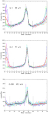 |
Fig. A.1. Mean profile (thick black line) obtained as outputs of our averaging method with only twelve superposed bursts (colored histograms). The top panel is relative to the G-1 data series at 4.5 keV, the central panel to the G-2 observation at 7.5 keV and the bottom panel to the G-3III observation at 13.2 keV. |
We verified the quality of the computed mean profiles by evaluating the linear correlation coefficients between the individual bursts and the mean profile for all the series of each energy channel. These correlation coefficients resulted very high; their average values are always higher than 0.94 for G-1 and G-2 data sets, and than 0.92 for G-3, with the exception of the highest energy channel for which we found 0.879. Standard deviations were always lower than 0.033 and for many series lower than 0.01.
This procedure generally maintains the individual bin content, so that the statistical properties are preserved. However, because the burst duration depends mainly on that of the SLT, it is possible that after the alignment a few bins of the final part of the preceding burst are occasionally superposed onto the initial bins of the subsequent one. This superposition can affect only a few bin in the initial and final segments of the mean profile, and to avoid any possible bias we eliminated the spurious data from the calculations of the means. These changes, however, are very small and limited to a few bins without any modification of the peak structures. Another advantage of this procedure is that the lengths of individual bursts are not altered and that the separations between peaks are preserved. Only a small number of bursts has large apparent deviations from the mean profile and those with the low correlation coefficients generally exhibit a broad pulse and the maximum is reached a few bin before the mean one. Regardless such large differences, these bursts were not excluded from the averaging calculations.
All Tables
Spectral best-fit parameter values for the baseline level (BL) data of the G-2 and G-3III spectra with the model TBABS*SIMPL*EZDISKBB.
Results of the phase resolved spectral analysis of the G-2 and G-3III spectra with the model TBABS*SIMPL*(EZDISKBB+BBODY).
All Figures
|
Fig. 1. Segments of the observations at the energy of 4.1 keV with a time bin size of 0.5 s: G-1 observation is shown in the left panel, G-2 in the central panel, and G-3 in the right panel. The vertical red lines mark the position of the maxima to better illustrate the variations in the duration of the bursts. We note that the time separation between vertical lines is not constant and that the peaks present different shapes in the three observations. |
| In the text | |
|
Fig. 2. Fourier periodogram of the entire observations at the energy of 4.1 keV with a time bin size of 0.5 s. The plot in the top panel is relative to G-1, that in the central panel to G-2 and the one in the bottom panel to G-3. The period values corresponding to the peaks are reported here. |
| In the text | |
|
Fig. 3. Short segments of the G-1 (top panel), G-2 (central panel) and G-3 (bottom panel) observations in different energy channels showing three consecutive bursts with a time binning of 0.5 s. The count rate has been scaled to be in the range 200–600 counts per bin. The horizontal lines correspond to the level of 350 counts per bin used for the selection of the folding phase marked with the vertical green lines. |
| In the text | |
|
Fig. 4. Normalized mean pulse profiles in three energy channels. Individual bursts are aligned at the point of the decay portion marked by the green vertical lines. The time binning is 0.5 s. Top panel: mean profiles for the G-1 data. Central panel: mean profiles for the G-2 data. Bottom panel: mean profiles for the G-3 data. The three peaks, P1, P2, and P3, are indicated with labels. |
| In the text | |
|
Fig. 5. Two mean profiles at different energies of the G-3 data set. The three bins that are indicated as wide, colored areas are the ones used for computing the peak amplitudes ratios. |
| In the text | |
|
Fig. 6. Peak amplitude ratios of P2 and P3 to P1 vs. photon energy. Dashed and dash-dotted lines are the linear best fit. |
| In the text | |
|
Fig. 7. Mean burst profile of the structure of the P3 feature in the three observations. The upper panel is relative to G-3 data in the energy range [9.1–15.1] keV. The blue line defines the constant level used for computing the excess and statistical errors in each bin (0.5 s width) are reported, the dashed line is the linear extrapolation of the last two bins along the P3 profile. In the lower panel profiles relative to G-1 and G-2 are shown, with the energy ranges corresponding to the five highest energy channels: [8.6–13.0] and [7.8–12.9] keV, respectively. |
| In the text | |
|
Fig. 8. Comparison of five mean profiles of P3 from the G-3III observation in the energy channels in the band [6.8–14.4] keV, normalized in amplitude assuming the maxima equal to 100. Black filled circles are the mean values and the error is the dispersion of these values and the dashed line is the plot of the given best fit formula. The black vertical line indicates the position of the maximum computed applying the same best fit law. |
| In the text | |
|
Fig. 9. Segments of normalized mean profiles. In the upper panel three normalized mean profiles of the G-1 bursts at the energies of 2.5 (thick black line), 7.5 (thin blue line), and 12.5 keV (red thick line) are shown. Short vertical lines mark the maxima of P1 and the long vertical line marks the shoulder. The lower panel presents segments of normalized mean profiles of the G-3III bursts in some energy channels from the lowest (3.5 keV, thick black line) to the highest one (14.4 keV, red thick line). Long vertical lines mark the maxima of P2 and the minima in valley between P1 and P2; short vertical lines mark the maxima of P1 at the extreme energies. We note the constant time distance between the minimum between P1 and P2, the maxima of P2 and P3, while the time of the P1 maximum shifts by 2.5 s. |
| In the text | |
|
Fig. 10. Time separation between the maxima of P2 and P1 (red filled circles) and the HXD (dark green filled diamond) of the G-3 data set. The dashed and the dot-dashed lines are the linear best fits to these sets. |
| In the text | |
|
Fig. 11. Best-fit values of kT (dark green filled circles) and Γ (blue filled triangles) of the BL and peak spectral best fits of the G-3III observation. Reported errors correspond to 1 standard deviation. Mean pulse profile at the energies of 4.1 (black) and 13.2 (red) keV to show the time correspondences are plotted. |
| In the text | |
|
Fig. 12. Best-fit spectral components of the three peaks of the G-3III data set, including the low energy absorption and the Comptonization to a power law. We note the increasing blackbody temperature from P1 to P3. Statistical uncertainties of the data are two orders of magnitude lower the values and are not visible in these plots. Top panel: black diamonds and deconvolved data for P1 and the black solid line is the total flux resulting from the sum of the EZDISKBB (red) and BBODY (blue) lines; central panel: same model for P2; bottom panel: same model for P3; we note the high energy flattening due to the Compton scattered photons. |
| In the text | |
|
Fig. A.1. Mean profile (thick black line) obtained as outputs of our averaging method with only twelve superposed bursts (colored histograms). The top panel is relative to the G-1 data series at 4.5 keV, the central panel to the G-2 observation at 7.5 keV and the bottom panel to the G-3III observation at 13.2 keV. |
| In the text | |
Current usage metrics show cumulative count of Article Views (full-text article views including HTML views, PDF and ePub downloads, according to the available data) and Abstracts Views on Vision4Press platform.
Data correspond to usage on the plateform after 2015. The current usage metrics is available 48-96 hours after online publication and is updated daily on week days.
Initial download of the metrics may take a while.