| Issue |
A&A
Volume 649, May 2021
|
|
|---|---|---|
| Article Number | A152 | |
| Number of page(s) | 18 | |
| Section | Extragalactic astronomy | |
| DOI | https://doi.org/10.1051/0004-6361/202038944 | |
| Published online | 01 June 2021 | |
The ALPINE-ALMA [CII] survey
Obscured star formation rate density and main sequence of star-forming galaxies at z > 4
1
Max-Planck-Institut für Astronomie, Königstuhl 17, 69117 Heidelberg, Germany
e-mail: This email address is being protected from spambots. You need JavaScript enabled to view it.
2
Aix Marseille Université, CNRS, LAM (Laboratoire d’Astrophysique de Marseille) UMR 7326, 13388 Marseille, France
3
IPAC, California Institute of Technology, MC 314-6, 1200 E. California Blvd., Pasadena, CA 91125, USA
4
Cosmic Dawn Center (DAWN), Copenhagen, Denmark
5
Observatoire de Genève, Université de Genève, 51 Ch. des Maillettes, 1290 Versoix, Switzerland
6
Kavli Institute for the Physics and Mathematics of the Universe, The University of Tokyo, 277-8583 Kashiwa, Japan
7
Department of Astronomy, School of Science, The University of Tokyo, 7-3-1 Hongo, Bunkyo, Tokyo 113-0033, Japan
8
Dipartimento di Fisica e Astronomia, Università di Padova, Vicolo dell’Osservatorio 3, 35122 Padova, Italy
9
Caltech Optical Observatories, California Institute of Technology, Pasadena, CA 91125, USA
10
Università di Bologna, Dipartimento di Fisica e Astronomia, Via Gobetti 93/2, 40129 Bologna, Italy
11
Istituto Nazionale di Astrofisica: Osservatorio di Astrofisica e Scienza dello Spazio di Bologna, Via Gobetti 93/3, 40129 Bologna, Italy
12
Instituto de Investigación Multidisciplinar en Ciencia y Tecnología, Universidad de La Serena, Raúl Bitrán 1305, La Serena, Chile
13
Departamento de Astronomía, Universidad de La Serena, Av. Juan Cisternas 1200 Norte, La Serena, Chile
14
Centro de Astronomía (CITEVA), Universidad de Antofagasta, Avenida Angamos 601, Antofagasta, Chile
15
INAF – Osservatorio Astrofisico di Arcetri, Largo E. Fermi 5, 50125 Firenze, Italy
16
Space Telescope Science Institute, 3700 San Martin Drive, Baltimore, MD 21218, USA
17
Cavendish Laboratory, University of Cambridge, 19 J. J. Thomson Ave., Cambridge CB3 0HE, UK
18
Kavli Institute for Cosmology, University of Cambridge, Madingley Road, Cambridge CB3 0HA, UK
19
Department of Physics and Astronomy, University College London, Gower Street, London WC1E 6BT, UK
20
Department of Physics and Astronomy, University of California, Davis, One Shields Ave., Davis, CA 95616, USA
21
Department of Astronomy, Cornell University, Space Sciences Building, Ithaca, NY 14853, USA
22
INAF-Osservatorio Astronomico di Padova, Vicolo dell’Osservatorio 5, 35122 Padova, Italy
23
Niels Bohr Institute, University of Copenhagen, Lyngbyvej 2, 2100 Copenhagen, Denmark
Received:
16
July
2020
Accepted:
1
February
2021
Abstract
Star formation rate (SFR) measurements at z > 4 have relied mostly on the rest-frame far-ultraviolet (FUV) observations. The corrections for dust attenuation based on the IRX-β relation are highly uncertain and are still debated in the literature. Hence, rest-frame far-infrared (FIR) observations are necessary to constrain the dust-obscured component of the SFR. In this paper, we exploit the rest-frame FIR continuum observations collected by the ALMA Large Program to INvestigate [CII] at Early times (ALPINE) to directly constrain the obscured SFR in galaxies at 4.4 < z < 5.9. We used stacks of continuum images to measure average infrared luminosities taking both detected and undetected sources into account. Based on these measurements, we measured the position of the main sequence of star-forming galaxies and the specific SFR (sSFR) at z ∼ 4.5 and z ∼ 5.5. We find that the main sequence and sSFR do not significantly evolve between z ∼ 4.5 and z ∼ 5.5, as opposed to lower redshifts. We developed a method to derive the obscured SFR density (SFRD) using the stellar masses or FUV-magnitudes as a proxy of FIR fluxes measured on the stacks and combining them with the galaxy stellar mass functions and FUV luminosity functions from the literature. We obtain consistent results independent of the chosen proxy. We find that the obscured fraction of SFRD is decreasing with increasing redshift, but even at z ∼ 5.5 it constitutes around 61% of the total SFRD.
Key words: galaxies: high-redshift / galaxies: evolution / galaxies: star formation / submillimeter: galaxies
Deceased.
© Y. Khusanova et al. 2021
 Open Access article, published by EDP Sciences, under the terms of the Creative Commons Attribution License (https://creativecommons.org/licenses/by/4.0), which permits unrestricted use, distribution, and reproduction in any medium, provided the original work is properly cited.
Open Access funding provided by Max Planck Society.
1. Introduction
The evolution of the star formation rate density (SFRD) is one of the fundamental elements for properly describing the history of the Universe. This measure provides both information about the in situ growth of galaxies and an inference for the number of ionizing photons produced by galaxies, helping to place constraints on the history of reionization (e.g., Madau & Dickinson 2014; Bouwens et al. 2015a; Robertson et al. 2015; Dayal & Ferrara 2018).
The SFRD is generally measured by converting the dust-corrected far-ultraviolet (FUV) luminosity density of galaxies (see e.g., Madau & Dickinson 2014). Since a fraction of the FUV light emitted by massive short-lived stars can be absorbed by dust, when present, the total SFRD consists of two components: the SFRDFUV, uncorr measured from the rest-frame FUV luminosity density and the dust-hidden component SFRDIR measured from the rest-frame infrared (IR) luminosity density.
The ratio between these two components changes with time and, hence, redshift. The obscured fraction, SFRDIR, dominates at low redshifts; it is three to ten times higher than SFRDFUV, uncorr at z < 3 (e.g., Sanders et al. 2003; Takeuchi et al. 2003; Magnelli et al. 2011, 2013; Burgarella et al. 2013). At a higher redshift, the SFRDIR is poorly constrained. However, since metals are produced by stars, the first galaxies should have very low dust content that is slightly enriched by only Population III stars. Therefore, in these galaxies, SFRDFUV, uncorr should be well in excess of the dust-hidden fraction SFRDIR. As star formation continues, stars internal to the galaxy begin to generate more dust. While the survival of dust grains is regulated by a series of constructive and destructive processes (Calura et al. 2017), the net result is an increase in the SFRDIR in respect to the SFRDFUV, uncorr. However, it is still unknown how fast the SFRDIR increases at early times and when it overcomes SFRDFUV, uncorr, mainly due to the lack of large, statistically-representative galaxy populations observed and selected both in the FUV and far-infrared (FIR) at high redshift (Dayal & Ferrara 2018).
Only a few attempts to constrain the SFRDIR at high redshifts exist in literature and their results remain inconclusive. Gruppioni et al. (2013) measured SFRDIR up to z ∼ 4 using Herschel selected galaxies and found that the SFRDIR decreases rapidly at z > 3. Wang et al. (2019a) extended these results to higher redshifts using the de-blended Herschel-SPIRE catalog. Their results show that the dust-obscured SFRD is comparable to estimates from the rest-frame UV at z ∼ 4−6. Rowan-Robinson et al. (2016) used the 500 μm sources from Herschel and found that the SFRDIR at z = 3−6 is even higher than the estimates from the rest-frame UV, although these results still have significant uncertainty. The measurements of Koprowski et al. (2017) using SCUBA-2 data at a redshift up to z ∼ 5, on the other hand, suggest a very steep decrease in SFRDIR (see discussion in Gruppioni & Pozzi 2019), so that SFRDIR at z > 4 is even lower than SFRDFUV, uncorr. This may be difficult to reconcile with the estimates of Rowan-Robinson et al. (2016) as well as with individual detections of very dusty galaxies at redshifts z ≃ 7 (Strandet et al. 2017; Bowler et al. 2018), z = 8.312 (Tamura et al. 2019), and z = 8.38 (Laporte et al. 2017), where the IR contribution should be extremely low if the SFRDIR continues to decrease rapidly with an increasing redshift. As the discoveries of individual, highly dust-obscured objects are not from volume-complete samples, it is difficult to determine whether such objects are common in the early Universe. However, the recent study using a volume-complete sample from the CO Luminosity Density at High Redshift (COLDz) survey by Riechers et al. (2020) resulted in the detection of three massive dusty starburst galaxies over ∼200 000 Mpc3, indicating a high space density of such dusty objects at z > 5. Since this study was limited to luminous starburst galaxies, this is only a lower limit and less luminous galaxies can contribute even more to SFRDIR. Previously mentioned studies based on measured IR luminosity functions (Gruppioni et al. 2013; Wang et al. 2019a; Rowan-Robinson et al. 2016; Koprowski et al. 2017) take this contribution into account; however, the observations at z > 3.0 rely on complex completeness corrections and difficult redshift identifications. In addition, they do not probe low luminosities, resulting in a poorly constrained faint end of the IR luminosity function. As such, conclusions related to the relative contribution of unobscured and obscured star formation at these epochs must be taken with caution and require confirmation through independent methods.
To overcome the difficulty of computing IR luminosity functions at z > 4, the measurements of the cosmic infrared background (CIB) produced by dusty galaxies can be used together with the modeling of dusty galaxy clustering, from which the SFRDIR can then be derived. Maniyar et al. (2018) did this analysis using the CIB anisotropy measurements and their cross-correlation with cosmic microwave background lensing (see also Planck Collaboration XXX 2014). The results are consistent with a shallower evolution of the SFRDIR at high redshifts compared to the results by Gruppioni et al. (2013) and Koprowski et al. (2017). At z > 4, the SFRDIR does not drop below SFRDFUV, uncorr but approaches it up to z ∼ 6.
Due to the difficulty in constraining the SFRDIR at redshifts z > 4, the measurements of the total SFRD rely mostly on the rest-frame FUV part of the spectrum. To account for the obscured fraction, the relation between the IR excess (IRX) and the UV spectral slope (β) is often used (Meurer et al. 1999). However, stacking analysis (Fudamoto et al. 2017), as well as individual observations of high redshift galaxies with Atacama Large Millimeter/submillimeter Array (ALMA), reveal significant scatter of dust properties. Most galaxies show a deficit of FIR flux compared to local galaxies with the same β slopes (Capak et al. 2015; Bouwens et al. 2016; Fudamoto et al. 2020), which can be partially explained by higher dust temperatures (Faisst et al. 2017). The measurements of dust temperatures are scarce at high redshifts but they show that dust temperatures are, indeed, higher than in local galaxies (30–43 K at z ∼ 5, Faisst et al. 2020). Since measurements of the SFRs at high redshifts are based on dust corrections coming from the IRX-β relation, the scatter in the relation induces uncertainties on these measurements. For this reason, observing rest-frame FIR continuum coming from galaxies selected in UV is important to independently constrain the IR luminosity density produced by these galaxies.
It is well established in the literature that star-forming galaxies form a so-called main sequence, a relationship between the amount of stellar mass in situ (M*) and the star formation rate (SFR, Noeske et al. 2007; Daddi et al. 2007; Whitaker et al. 2012; Speagle et al. 2014; Salmon et al. 2015; Tasca et al. 2015; Schreiber et al. 2015; Tomczak et al. 2016; Santini et al. 2017; Pearson et al. 2018; Khusanova et al. 2020). However, the measurements of the SFRs of individual galaxies at z > 4 suffer from the uncertainty of the IRX-β relation and/or the dust temperature of the galaxies. Hence, a lower number of galaxies is detected in the rest-frame FIR than expected assuming local IRX-β relation (e.g., Capak et al. 2015; Bouwens et al. 2016). Besides, getting a wide volume in the rest-frame FIR at z > 4 is expensive observationally. Therefore, the constraints on the main sequence of galaxies are limited and are mostly based on the rest-frame FUV data.
Only a few attempts have been made to constrain the main sequence using submillimeter observations, mainly using data from Herschel (Schreiber et al. 2015; Pearson et al. 2018). At z > 4, however, the measurements are limited by confusion noise (Nguyen et al. 2010), which makes it difficult to observe individual sources without careful and well-informed de-blending schemes. Therefore, these works primarily are limited to only the high mass end of the main sequence (log(M*/M⊙) > 10.5). Star-forming galaxies with such high masses are rather rare, and it remains unclear if the slope of the main sequence remains the same over the whole range of masses.
The main sequence evolution with redshift is linked to the sSFR evolution defined as SFR/M*, although the sSFR evolution can vary depending on the mass if the slope of the main sequence is not unity, as claimed in several studies (e.g., Salmon et al. 2015; Schreiber et al. 2015; Tasca et al. 2015; Khusanova et al. 2020). In that case, the measurements from UV selected samples, which probe galaxies with lower stellar masses (log(M*/M⊙) ≲ 10) are not comparable with FIR samples probing higher stellar masses (Schreiber et al. 2015). The sSFR constraints at high redshifts are inconclusive: while many studies find a shallower evolution at high redshifts (Bouwens et al. 2012; González et al. 2014; Tasca et al. 2015; Faisst et al. 2016; Santini et al. 2017), some find higher sSFR, consistent with steeper evolution, as at lower redshifts (Stark et al. 2013; de Barros et al. 2014).
The ALMA Large Program to INvestigate [CII] at Early times (ALPINE) was designed with a goal of measuring the dust-hidden SFR in galaxies at z > 4 from a representative UV selected sample (Béthermin et al. 2020; Le Fèvre et al. 2020; Faisst et al. 2020). In this paper, we use a large sample of 118 galaxies observed in the rest-frame FIR with ALMA to determine the SFRDIR at z > 4 from ALPINE. We also determine their average and individual SFRs and constrain the main sequence over the stellar mass range 9 ≲ log(M*/M⊙) ≲ 11. Our goal is to estimate SFRs and SFRD without relying on the IRX-β relation and by directly measuring the total IR luminosities. We present the ALPINE data in Sect. 2. In Sect. 3, we describe the stacking code and the methods to measure the SFRD. In Sect. 4, we present and discuss our SFRD measurements. Section 5 is dedicated to a discussion about the main sequence and the sSFR evolution with redshift. In Sect. 6 we summarize our results.
Throughout the paper, we use a ΛCDM cosmology with ΩΛ = 0.70, Ωm = 0.30 and h = 0.7. All magnitudes are given in the AB system. We assume a Chabrier (2003) initial mass function (IMF) to convert luminosities to SFRs. We refer to absolute magnitude at 1600 Å by MFUV and total luminosity between 8 and 1000 μm by LIR.
2. Data
We use the data from ALPINE, a survey designed to observe [CII] emission and the rest-frame FIR continuum of a representative sample of star-forming galaxies in the redshift range 4.4 < z < 5.8 with a gap at redshifts 4.65 < z < 5.05, where the [CII] 158 μm emission line falls into a window of low atmospheric transmission (Le Fèvre et al. 2020). The galaxies are selected by the following criteria: UV-luminosity is above 0.6L* or MFUV < −20.2 (it is important to note that this selection is missing faint UV sources, the consequences of that are discussed below and in Sect. 4.3.3) and have secure spectroscopic redshifts from the rest-frame UV spectra. The secure spectroscopic redshift ensures that [CII], if present, falls within the relatively narrow observed ALMA bandpass. The redshifts are taken from two large spectroscopic surveys: VIMOS UltraDeep Survey (VUDS, Le Fèvre et al. 2015; Tasca et al. 2017) and DEep Imaging Multi-Object Spectrograph (DEIMOS, Faber et al. 2003) 10 K Spectroscopic Survey (Hasinger et al. 2018). The targets for these spectroscopic surveys are selected based on their broad and narrow band photometry. More on the selection can be read in Le Fèvre et al. (2020).
The advantage of the ALPINE selection is that it covers a wide range of stellar masses (9 ≲ log(M*/M⊙) ≲ 11) and SFRs derived from the rest-frame FUV with Spectral Energy Distribution (SED) fitting (1 ≲ log(SFR[M⊙ yr−1]) ≲ 3, Faisst et al. 2020). The targets are “normal” star-forming galaxies and, based on observations in the rest-frame FUV, populate the main sequence. We use stacking of both detections and nondetections to derive the average properties of the sample (see Sect. 3). In this way, we avoid bias toward rare, bright starburst galaxies, compared to other observations of samples selected in the rest-frame FIR at these redshifts. Since the targets are selected from well-studied fields, they are imaged with both space and ground-based instruments (Grogin et al. 2011; Koekemoer et al. 2011; Laigle et al. 2016; Skelton et al. 2014).
However, the ALPINE selection of targets has two caveats. First of all, since the selection is based on UV-properties of galaxies, the objects which are faint in UV are missed. Hence, their contibution is not taken into account by our SFRD measurements and blind surveys are still necessary to make a proper estimate of contribution from such objects. This caveat is discussed in more detail in Sect. 4.3.3. The second caveat is the bias toward higher UV-luminosities in the low mass bins. In Sect. 3.2.2, we discuss how we deal with this caveat in deriving the SFRD.
In total, 118 galaxies were observed in the period from May 2018 to January 2019 (see Béthermin et al. 2020). The ALMA data were calibrated with the standard ALMA pipeline. The Common Astronomy Software Applications (CASA) software was used for the data reduction (McMullin et al. 2007). To produce continuum maps, we excluded all the channels that correspond to the position of the [CII] line. In case of nondetections of the [CII] emission, we used spectroscopic redshifts from VUDS or DEIMOS 10K and excluded data within 500 km s−1 around the expected position of [CII] line. For galaxies with detected [CII] emission, we manually defined the window around the detected emission line. We then produced continuum maps, using the task tclean. We used natural weighting to maximize the signal-to-noise (S/N). More detail on data reduction can be found in Béthermin et al. (2020).
The survey was optimized to detect [CII] line emission. Therefore, the expected S/N for the rest-frame FIR continuum varies in the range from 0.5 to 3 for most targets based on the SED models of Béthermin et al. (2017). We reached a sensitivity of 50 μJy beam−1 at 4.4 < z < 4.6 and 28 μJy beam−1 at 5.1 < z < 5.8. We found that 95% purity is reached with a S/N = 3.5 cut for targeted galaxies. Only 23 out of 118 (19%) of the ALPINE targets are detected with such significance. However, given the known positions of the targets, we can extract the average continuum flux of nondetected galaxies using stacking, as described in Sect. 3.1.
The galaxies in ALPINE were chosen in the two well-studied fields, Cosmic Evolution Survey (COSMOS, 89% of targets, Scoville et al. 2007) and Extended Chandra Deep Field-South Survey (ECDFS, 11% of targets, Giacconi et al. 2002) that is covered by CANDELS (Koekemoer et al. 2011; Grogin et al. 2011). The photometry from the public COSMOS catalog (Laigle et al. 2016) was used for targets in the COSMOS field, and the 3D-HST catalog (Skelton et al. 2014) was used for the ECDFS. Faisst et al. (2020) analyzed the multiwavelength ancillary data in both fields and derived the physical properties of galaxies using SED fitting at fixed spectroscopic redshift (stellar masses, SFRs, rest-frame FUV luminosities, etc.).
The SED fitting was performed with the LePhare package (Arnouts et al. 1999; Ilbert et al. 2006) as well as a modified version of the HyperZ code (Bolzonella et al. 2000), using Bruzual & Charlot (2003) models. The model parameters are outlined in Table 1. The fitting was performed in flux density space and emission lines were included. The two different codes were used to analyze the systematic uncertainties introduced by the χ2 minimization algorithms and the treatment of emission lines (see Faisst et al. 2020). The absolute UV magnitudes from the two codes agree, while the stellar masses and SFRs have systematic uncertainties of ∼0.3 dex. Only four galaxies were found to have significantly different (larger than systematic uncertainties) stellar masses and SFRs due to contaminated Spitzer photometry. The derived physical parameters were compared to previous results for the galaxies in COSMOS field derived with photometric redshifts and we found that they agree. Here and in other ALPINE papers, we use the parameters derived by the SED fitting derived with LePhare. More details about the SED fitting of ALPINE galaxies and ancillary data can be found in Faisst et al. (2020).
Model parameters for SED fitting.
3. Methods
3.1. Stacking of the rest-frame FIR continuum images
As mentioned above, for ∼81% of the ALPINE targets, the observed continuum flux cannot be measured since it falls below the 3.5σ limits. Therefore, we use stacking to measure the average flux of galaxies with similar physical properties. We use all the targeted galaxies including both detections and nondetections, since our goal is to get the average flux of the whole population of galaxies in each bin.
Here we use the mean stacks of continuum images. We only use the targeted galaxies and their UV-positions for alignment. Since the targets are not perfectly aligned on stacks due to uncertainties in astrometry or real physical offsets, the flux is measured using an aperture of 3 arcsec diameter. Béthermin et al. (2020) has tested three other methods of continuum flux measurements in addition to aperture photometry: Gaussian fitting on a continuum map and on the UV plane, and peak flux. They all were proven to be consistent with each other, except for the peak flux. This is because the sources are not point-like. However, on stacks only aperture photometry can be used, since we cannot align the nondetected sources and their sizes can vary from target to target. Therefore, their mean profile is not Gaussian. The aperture photometry, on the other hand, makes it possible to measure the flux without any assumption on the profile shape. Since the beam sizes in ALPINE do not exceed 1.6 arcsec, the 3 arcsec aperture is large enough to include all the flux from the targets even if the sources are significantly extended. Fujimoto et al. (2020) examined the radial surface brightness profiles of ALPINE targets and found that the sources are compact in the rest-frame FIR.
We use bootstrapping analysis to ensure the robustness of the measurements of the flux and to estimate the uncertainties coming from both the noise and the sample variance. Each stack is produced from a set of continuum images. To measure the average flux and its uncertainty, we randomly draw a new sample of images without withdrawal from the initial set and produce a new stack image, from which the continuum flux is remeasured. We repeat the procedure 1000 times and find the average and standard deviation of the measurement – σboot.
We also measure the flux in the field with the same aperture at each step. We mask the positions of the serendipitously detected objects and the center beforehand, to ensure that the flux measured in the field is not contaminated. The apertures are then placed at random positions, away from serendipitous sources. The variance of the field flux is an estimate of the photometric noise on the stacked image and is on average σphot = 50 μJy for the typical number of stacked images (eight). The average flux in the field is compatible with zero as expected (Ffield = 0.1 ± 50.0 μJy).
As discussed in Béthermin et al. (2012), the bootstrap uncertainty σboot and the photometric noise σphot are related as:
 (1)
(1)
where Nstack is the number of images in the stack and σpop is the intrinsic population variance. The uncertainties derived using the bootstrap method are thus including both the photometric noise and the sample variance coming from the finite size and the possible large heterogeneity of the stacked samples.
In order to test reliability of the flux measurement on the stacks, we generated a number of fake sources on the images avoiding the center with fluxes drawn from a Gaussian distribution with a known mean Fin and variance σin. The sources are Gaussian and their FWHM were allowed to vary from 0.8 to 1.6 arcsec (as the beam sizes in ALPINE, Béthermin et al. 2020). We used the procedure described above to stack images with the fake sources, but in order to simulate position uncertainties of real targets, we added random offsets sampled from a Gaussian with σ = 0.12 arcsec (as the average astrometric offset of ALPINE targets, Faisst et al. 2020). Then we measured the average flux Fout and the bootstrap uncertainty σout. We performed the procedure 250 times, varying the Fin flux value in the range 10–180 μJy or ∼0.25–3.5σphot and the number of images from six to 13 (as we used later for the stacks).
Figure 1 shows the distribution of ΔF/σout = (Fout − Fin)/σout. The mean of the distribution is −0.03 and the standard deviation is 1.13. The mean is compatible with zero. The standard deviation of the distribution can be reduced to ∼1, if we limit the analysis to stacks with a high number of images (> 20), however, this is not feasible given the number of objects in the sample. We, therefore, divide the sample in smaller bins and make stacks with the number of objects in range from six to 13 to be able to constrain the LIR − M* or LIR − MFUV relation.
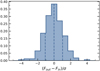 |
Fig. 1. Comparison of injected and recovered fluxes from stacking. The vertical dashed lines correspond to 16th, 50th and 84th percentiles of the distribution (−1.08, −0.02, 1.03). |
We cannot assess the real shape of the LIR distribution but the population variance can tell us how well the average LIR of a given selection is constrained. For instance, if the distribution is bimodal, our bootstrap procedure will measure a high population variance. These uncertainties taking into account both the population variance and the noise are propagated to the other derived quantities.
In conclusion, the average fluxes on stacks are well recovered within the error bars if the sources are not significantly extended or offset. This is the case for the detected targets (Béthermin et al. 2020). Therefore, stacking can be safely used to recover the average continuum fluxes.
3.2. SFRD measurement: Method description
The total SFRD can be defined as (see e.g., Madau & Dickinson 2014):
 (2)
(2)
where SFRDFUV, uncorr is derived from the FUV luminosity density (ρFUV) not corrected for dust attenuation, and SFRDIR is derived from the IR luminosity density (ρIR). The conversion factors are κFUV = 1.5 * 10−10 M⊙ yr and κIR = 10−10 M⊙ yr
 for Chabrier (2003) IMF (Kennicutt 1998).
3.2.1. Measuring IR luminosity density
Since ALPINE is not a volume-limited sample, it is rather difficult to determine the IR luminosity function from the target sample (see Gruppioni et al. 2020, for IR luminosity function measurement based on nontarget galaxies found in ALPINE). We use, therefore, a different approach to obtain the IR luminosity density, which can then be converted to the SFRDIR. The method is based on using some physical property as a proxy of the IR luminosity – LIR and convolving the volume density distribution of this proxy with the mean LIR-proxy relation as:
 (3)
(3)
where x is a proxy (MFUV or M*, see Sect. 3.2.2), ⟨LIR⟩ is the total IR luminosity and ϕ(x) is either the FUV luminosity function (UVLF) or the galaxy stellar mass function (GSMF). The total IR luminosity is derived from the SED templates scaled to the 158 μm flux measured on stacks and then integrated from 8 to 1000 μm. We use average conversion factors ⟨ftemp, z ∼ 4.5⟩ = 0.13 ± 0.02 and ⟨ftemp, z ∼ 5.5⟩ = 0.12 ± 0.03 derived from a set of templates from the literature, which are consistent with the stacked Herschel data (see Appendix A for more detail on the templates and conversion factors). The volume density distribution can be derived from the literature measurements of the proxy density functions (UVLF or GSMF in our case). A summary of the method is presented in Fig. 2.
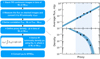 |
Fig. 2. Illustration of the method used to determine the SFRDIR. Left panel: steps performed. Right panel: arbitrary proxy density function (UVLF or GSMF) and a power law relation between the property used as a proxy and the FIR flux. The black squares represent measured values and the solid line the fit with uncertainties represented by a shaded region. The vertical shaded regions show the proxy range, in which the data is available for both the power law relation derived from ALPINE and the proxy density function. |
3.2.2. The choice of proxy
The method described above relies on the assumption that there is a relation between the proxy and the IR luminosity. To first order, this is true for stellar masses (M*, we refer to “stellar mass” as “mass” hereafter) of star-forming galaxies, which sit on the main sequence. Their SFR increases with the mass (Whitaker et al. 2012, 2014; Tasca et al. 2015; Salmon et al. 2015; Santini et al. 2017; Pearson et al. 2018; Khusanova et al. 2020). While it is still unclear what fraction of SFR is hidden by dust, we expect that there is a relation between the masses and the IR dust emission (this is further discussed in Sect. 5 dedicated to the main sequence). Also the FUV-magnitudes are linked to SFR to first order. If we assume that more star-forming galaxies have higher IR luminosities, the FUV-magnitudes should correlate with the LIR. Each proxy, however, has its own sources of uncertainty, which are discussed below. Therefore, we use both of them and compare the results.
The accuracy of the mass is limited, since it is derived from SED fitting and it is, therefore, model-dependent. The caveat in using the mass as a proxy is the fact that the sample of galaxies in ALPINE is selected to have FUV luminosities above 0.6L*. Hence, the galaxies selected at lower masses are not representative of typical galaxies at these masses, since they are biased toward higher UV luminosities at fixed mass. We show in Fig. 3 the median values of the M* − MFUV relation from Salmon et al. (2015) and the fit of this relation. This relation agrees well with the M* and MFUV measurements for ALPINE targets. We find the mass at which the 1σ envelope around the best fit crosses the FUV luminosity selection limit, where σ is the scatter around the fit. As shown in Fig. 3, the mass limit is log Mlim/M⊙ = 9.6 at both redshifts. Below this limit we are likely to miss galaxies with faint FUV magnitudes, biasing SFR toward higher values.
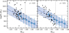 |
Fig. 3. Stellar mass versus FUV magnitude. The black circles are ALPINE targets as measured by Faisst et al. (2020). The open squares are measurements from Salmon et al. (2015). The solid blue line is the fit to the measurements by Salmon et al. (2015) and the shaded areas are 1σ uncertainties. The vertical dotted line shows the FUV luminosity cut used in selecting galaxies. The vertical dotted lines show the mass limits below which the flux measurements are considered to be upper limits. Left panel: z ∼ 4.5 redshift bin and right panel: z ∼ 5.5 bin. |
The FUV magnitudes are not affected by this bias. Since the spectroscopic redshifts are known, they are not model-dependent and can be derived with high accuracy given well-measured photometry (Faisst et al. 2020). We do not correct the derived FUV magnitudes for dust attenuation in order to keep them model-independent. However, the more dust is in the galaxy, the more FUV radiation is absorbed for a given SFR/IMF combination. Therefore, even if majority of faint in FUV galaxies have low dust content, some dust rich galaxies can contaminate FUV faint bins. In that case, the population will be heterogeneous in each bin and the relation may have larger scatter. This will make it more difficult to constrain the relation between FUV magnitude and IR luminosity. We determine the population variance with the bootstrapping procedure described in Sect. 3.1 (see Eq. (1)). The impact of the population variance is then propagated to the uncertainties on the SFRD. However, if the population variance is intrinsically too large, the use of FUV magnitudes as a proxy can be challenging to analyze small samples.
3.2.3. Integration limits
ALPINE probes only a range of masses (9 ≲ log(M*/M⊙) ≲ 11) or FUV-magnitudes (−19 ≲ log(M*/M⊙) ≲ − 23), used as a proxy (this range is schematically shown as shaded region in Fig. 2). In this range, we have measurements of the rest-frame FIR flux directly from the stacks of ALPINE images. The proxy density is known from observations. The SFRDIR measured from integration in this range is, hence, the most robust lower limit of the dust-hidden fraction of SFRD. However, more IR luminosity can be contained in FUV faint or low mass galaxies. While these galaxies are expected to have low dust content, they can still affect the results due to their high density in the Universe. Galaxies with high masses or bright in FUV are rare, but they also contribute to the total SFRD budget. Therefore, we need to extrapolate the observed LIR-proxy relation and the proxy density functions to obtain the estimate of the total SFRDIR.
We determine, first, the lower limit (SFRDIR, min) by integrating the Eq. (3) within the observed in ALPINE mass or FUV-magnitude range. Then, for the extrapolation, we use the integration limits corresponding to 0.03L*1 and 100L*. These are MFUV = −17 and MFUV = −26, respectively. In order to define integration limits for masses, we convert these limits to SFRs. Then we use the relation between SFR and mass from the main sequence fit in Khusanova et al. (2020) to find the corresponding masses: log(M*/M⊙) = 6.0 for the lower limit and log(M*/M⊙) = 12.4 for the upper limit. With these limits, we can make a meaningful comparison between the SFRDFUV, uncorr derived in the literature from UVLFs and the SFRDIR measured here. We note that even after extrapolation, we are missing galaxies with high IR luminosity, because some of them are too faint in the rest-frame FUV to be detected in current photometric surveys (e.g., Caputi et al. 2014; Franco et al. 2018; Williams et al. 2019; Wang et al. 2019b; Gruppioni et al. 2020). Their contribution is discussed in the Sect. 4.3.3.
4. SFRD measurement results
4.1. Proxy number density
First, we need to define the proxy number density: UVLF or GSMF. Their measurements are widely available in the literature (e.g., Bouwens et al. 2015b; Finkelstein et al. 2015; Ono et al. 2018; Pelló et al. 2018; Khusanova et al. 2020; Song et al. 2016; Davidzon et al. 2017; Wright et al. 2018) but are still affected by many uncertainties. In particular, the faint and low mass end slopes are still not well constrained. Another uncertainty is the shape of the UVLF. While most authors assume the Schechter function form, some recent works find that at high redshift the double power law (DPL) is preferable form (Bowler et al. 2015; Ono et al. 2018; Khusanova et al. 2020). We do not favor any particular UVLF or GSMF, but use several of them to show how the uncertainties on their parameters and functional form propagate into our SFRD estimates.
For the UVLF, we use the Bouwens et al. (2015b), Finkelstein et al. (2015), Ono et al. (2018), Pelló et al. (2018) and Khusanova et al. (2020) results. The Bouwens et al. (2015b), Finkelstein et al. (2015) and Pelló et al. (2018) UVLFs are based on large samples with photometric redshifts. The UVLF is represented with a Schechter function. Ono et al. (2018) uses a dropout selection partially confirmed by spectroscopic redshifts and Khusanova et al. (2020) uses the sample with spectroscopic redshifts. These studies probe the bright end of the UVLF and find a DPL form of UVLF.
We use Song et al. (2016), Davidzon et al. (2017) and Wright et al. (2018) measurements of GSMFs. Song et al. (2016) GSMFs are based on samples selected from CANDELS-GOODS field. Davidzon et al. (2017) uses photometric selection of galaxies in COSMOS field, and Wright et al. (2018) uses a joint analysis of GAMA, COSMOS, and 3D-HST data. We note that the physical parameters derived for ALPINE galaxies in COSMOS field were compared with the COSMOS15 catalog and are consistent (see Faisst et al. 2020). Therefore, the uncertainties of mass measurements, which are more affected by the choice of the IMF and star formation history (SFH) in SED fitting compared to FUV magnitudes, should not have impact on our results, when we combine the COSMOS-based GSMF with LIR-mass relation from ALPINE.
4.2. Infrared luminosity as a function of proxy
As discussed in Sect. 3.2.2, we used two proxies in this work: masses and FUV magnitudes derived using the SED fitting as described in detail in Faisst et al. (2020). The bin sizes were chosen to be small enough to reduce the heterogeneity of the underlying population but to include enough galaxies (6-13) in the bin to have robust average flux measurements. As was discussed in Sect. 3.1, even faint fluxes on the stacks give us information on the average flux of the underlying population of galaxies. Therefore, we use 3.5σphot upper limits only when the measured fluxes of the stack have negative values. In such cases, we use conservative upper limits 0+3.5σphot. In all the remaining cases, we use the average flux measured with bootstrapping (the S/N in these cases is > 0.5σphot). When stacking by mass bins, we consider the results as upper limits in bins below log Mlim/M⊙ = 9.6, for the reasons discussed in Sect. 3.2.2 (bias toward higher SFR because of the FUV selection of ALPINE). The upper limits in those cases are the sum of the flux measured on stacks and 3σ.
We converted the average rest-frame 158 μm fluxes to ⟨LIR⟩ and found the ⟨LIR⟩-proxy relation. We show the resulting relations in Fig. 4. The ⟨LIR⟩ is clearly well correlated with both proxies. We fit this relation with a power law using the MCMC method with emcee package in python and checking at each step that the fit does not go above upper limits. The results are shown in Fig. 4. The slope is well constrained, and the normalization lies within the error bars. We use the MCMC chains later when deriving the SFRDIR. This allows us to derive the uncertainty of the SFRDIR measurements, which relies on the precision of our ⟨LIR⟩-proxy relation.
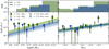 |
Fig. 4. Average infrared luminosity versus proxy (stellar mass as a proxy on the left panel and FUV magnitude on the right). The green squares and blue circles are the average IR luminosities on the stacks at z ∼ 4.5 and z ∼ 5.5, respectively. The black error bars show the population variance (σpop), the colored error bars show the photometric noise (σphot, see Eq. (1), Sect. 3.1). The open squares are the flux measurements on stacks below mass limit Mlim. The stars are the results on stacks excluding the galaxies with signs of possible contamination by a close companion. The green and blue dashed lines are the best fits of the relation and the thin lines of corresponding color are the MCMC chain realizations of the fit. Top panels: S/N on each stack. |
Faisst et al. (2020) identified galaxies with signs of possible contamination of photometry by close companions (based on optical HST and ground-based images). Excluding them lowers the number of galaxies which can be used for stacking, but does not affect the resulting power law relation between the proxy and ⟨LIR⟩. We show the results obtained from the stacks after excluding the galaxies with signs of contamination in Fig. 4. Since this new sample contains less objects, we had to adjust the bins, but the data points agree with the power-law relation found for the full sample.
In Fig. 4, we show the photometric errors and population variance computed as described in Sect. 3 (see Eq. (1)) and S/N in each stack. The population variance at z ∼ 4.5 is ∼0.91 dex on average. At z ∼ 5.5, it is ∼0.47 dex, almost two times lower. As discussed in Sect. 3.2.2, if the underlying population is heterogeneous, the scatter of its FIR properties will be large. This is what we observe at z ∼ 4.5. This makes the LIR − MFUV relation particularly difficult to constrain at z ∼ 4.5.
We note that the two points below Mlim, which were excluded from the fit due to a possible bias (see Sect. 3.2.2), are in a very good agreement with the power law fit to the points above Mlim. Therefore, we trust these two points and use them later, when we derive the main sequence.
Interestingly, we observe a stronger evolution with redshift of the LIR − M* relation than the LIR − MFUV relation. As the redshift decreases, the LIR on average increases for galaxies with the same mass, which means the dust attenuation increases in these galaxies.
4.3. Infrared contribution to SFRD
We present the results of our measurements of SFRDIR in Figs. 5 and 6 for redshifts z ∼ 4.5 and z ∼ 5.5 respectively, and in Table 2. Although the results depend on the choice of the proxy density parameters, in most cases they agree with each other within the error bars. The choice of the proxy plays a role in the constraining power of our method. At redshift z ∼ 4.5, the population variance in FUV bins is larger as we noted before. Hence, although we find a fit to the measured points, these constraints should be interpreted with caution. At z ∼ 5.5, on the contrary, we have weaker constraints when using the mass as a proxy. Due to the bias toward higher FUV magnitudes in low mass bins, we had to exclude them from the fitting of the LIR − M* relation. The remaining points have larger uncertainties at z ∼ 5.5. Hence, the fit of the LIR − M* relation has larger uncertainties, which propagate into uncertainties of the SFRD estimates.
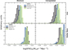 |
Fig. 5. Probability distribution of the SFRDIR at redshift z ∼ 4.5. All distributions are derived with the same relations between the stellar mass (bottom panels) and FUV magnitudes (top panels). The minimum is derived in the observed by ALPINE range of stellar masses and FUV magnitudes and is shown on the left panels. The SFRDs from extrapolated relation are shown on the right panels. Different colors correspond to different GSMFs and UVLFs (Bouwens et al. 2015b; Finkelstein et al. 2015; Ono et al. 2018; Davidzon et al. 2017; Song et al. 2016; Wright et al. 2018). |
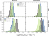 |
Fig. 6. Same as Fig. 5, but at redshift z ∼ 5.5. The UVLFs and GSMF are taken from Bouwens et al. (2015b), Pelló et al. (2018), Khusanova et al. (2020), Davidzon et al. (2017), Song et al. (2016), Wright et al. (2018). |
Infrared SFRD (log SFRDIR M⊙ yr−1 Mpc−3):
The measurements obtained with FUV as well as M* as a proxy agree well with each other within the errors in both redshift bins. The fact that the measurements obtained with different proxies are consistent with each other gives us certainty on robustness of our constraints of the IR contribution to the SFRD. In the next section, we discuss our measurements in the context of the SFRD evolution.
4.3.1. Lower limit of the obscured SFRD
First, we obtained the lower limit on SFRDIR. For that, we integrated the ⟨LIR⟩-proxy relation with the proxy density function in the range where both of them are known from the observations. Hence, this estimate is free from the uncertainties induced by extrapolations. The integration limits are 8.35 ≤ log(M*/M⊙) ≤ 10.5 for masses and −23.3 ≤ MFUV ≤ −20.0 for FUV magnitudes.
As described in Sect. 4.1 and 4.2, each power law function describing LIR-proxy relation is fit with the MCMC (see Eq. (3)). To derive the SFRDIR and its uncertainty, we use the MCMC chains of fit parameters to produce a resulting SFRDIR chain. In this way, we obtain a probability distribution function (PDF) of SFRDIR, which is a normalized distribution of individual SFRDIR measurements at each step. These PDFs are shown in the left panel of Figs. 5 and 6 for both proxies. Depending on the choice of the proxy density function, the PDFs differ but remain consistent within the error bars for each proxy. In Fig. 7, we show the lowest value minus 1σ as our lower limits for the IR contribution to SFRD. These are the most robust lower limits of the SFRDIR as they are obtained with a large and representative sample of galaxies at 4.4 < z < 5.8 and only using the proxy range, where actual observations are available.
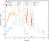 |
Fig. 7. Evolution of the total SFRD (Eq. (2)) with redshift. The red symbols are the total SFRDs, derived in this paper. Small offsets of ±0.08 are applied to their redshift for clarity. The triangles are the lower limits for SFRDIR derived in Sect. 4.3.1. The blue symbols are dust-corrected SFRD derived from the FUV data (Cucciati et al. 2012; Dahlen et al. 2007; Reddy & Steidel 2009; Bouwens et al. 2012, 2015b; Schenker et al. 2013; Pelló et al. 2018; Khusanova et al. 2020), orange symbols are derived from reradiated dust emission from forming stars as measured from the IR (Magnelli et al. 2013; Gruppioni et al. 2013, 2020; Rowan-Robinson et al. 2016; Koprowski et al. 2017; Wang et al. 2019a; Riechers et al. 2020). The magenta points are from other SFR tracers: [CII] luminosity function based on the ALPINE field sample of Loiacono et al. (2021) and number counts of γ-ray bursts (Kistler et al. 2009). The dotted line is the fit of SFRD evolution from Madau & Dickinson (2014). |
Given this lower limit, the IR contribution to the total SFRD is already at least 8–13% at z > 4 as compared to the total SFRD from the Madau & Dickinson (2014) curve. While this is seemingly a small amount, these results are in severe disagreement with the results by Koprowski et al. (2017). They fit the evolution of SFRDIR with redshift by the Gaussian function. The extrapolation of this curve gives log(SFRDIR M⊙ yr−1 Mpc−3) = −3.95 at z ∼ 5.5, which is much lower than the ALPINE lower limit at this redshift log(SFRDIR M⊙ yr−1 Mpc−3) = −2.67. Although, the agreement between ALPINE lower limits and SFRDIR measurements by Koprowski et al. (2017) could be reached by a shallower function at z > 4, we note that we only considered a small range of masses or FUV magnitudes for computing the lower limit of SFRDIR and our sample is UV-selected. Hence, the real values at both redshifts are even higher and in even stronger tension with Koprowski et al. (2017). Due to the fact that the work of Koprowski et al. (2017) is based on the IR luminosity functions, the observations in the high redshift bins barely cover the faint end slope of the IR luminosity function, whose uncertainty could be one of the sources of this discrepancy.
4.3.2. Extrapolated infrared star formation rate density
The total SFRDIR is higher than the lower limit derived above. To derive the total SFRDIR, we assume that the ⟨LIR⟩−proxy relation is the same at all FUV-magnitudes and masses and extrapolate the ⟨LIR⟩−proxy relation as well as the proxy number density function to the integration limits, corresponding to 0.03L* and 100L* or log(M*/M⊙) = 6.0 and log(M*/M⊙) = 12.4 for masses, as mentioned in Sect. 3.2. We obtain the PDFs in the same way as above and show the results on the right panels in Figs. 5 and 6. To place the results in the context of the SFRD evolution, we combine the PDFs obtained with different proxy density functions from the literature. Since the lengths are the same for all chains, combining them does not favor any particular proxy density function. We obtain an average estimate of the SFRD and our uncertainties naturally include the systematics coming from the GSMF and UVLF.
Figure 8 illustrates the evolution with redshift of SFRDIR and the uncorrected for dust estimate from FUV luminosity density – SFRDFUV, uncorr. We observe a gradual decrease in the SFRDIR, which only starts to intersect with the SFRDFUV, uncorr at z > 5. Even at such high redshifts, the SFRDFUV, uncorr does not overcome the SFRDIR. It remains an open question, however, at which redshift the SFRDFUV, uncorr overcomes the SFRDIR, since at z > 4 the SFRDIR is only gradually approaching the SFRDFUV, uncorr. If the evolution is flatter at higher redshifts, then the dust contribution becomes negligible compared to SFRDFUV, uncorr only at very high redshifts. This trend is consistent with the extrapolation of the Maniyar et al. (2018) model of SFRDIR evolution, which is based on CIB anisotropies. Our results agree well with this model at both redshifts. However, if the contribution from ultra-dusty objects, which are missing from the optical and near-infrared (NIR) catalogs is significant, the SFRDIR evolution can be even flatter.
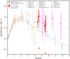 |
Fig. 8. Evolution of SFRDIR and SFRDFUV, uncorr with redshift. The red symbols are the SFRDIR, derived in this paper. Small offsets of ±0.08 are applied to their redshift for clarity. The triangles are the lower limits for SFRDIR derived in Sect. 4.3.1. The blue symbols are SFRDFUV, uncorr derived from the FUV data (Cucciati et al. 2012; Dahlen et al. 2007; Reddy & Steidel 2009; Bouwens et al. 2012, 2015b; Schenker et al. 2013; Pelló et al. 2018; Khusanova et al. 2020), orange symbols are SFRDIR from Magnelli et al. (2013), Gruppioni et al. (2013, 2020), Rowan-Robinson et al. (2016), Koprowski et al. (2017), Wang et al. (2019a) and Riechers et al. (2020). Orange lines are the fits of SFRDIR evolution from Koprowski et al. (2017) and Maniyar et al. (2018). |
Such objects, indeed, exist. For example, an ultra-dusty merging galaxy was discovered at z = 5.185 (Neri et al. 2014), and at even at higher redshift, z = 6.34 (Riechers et al. 2013). However, the individual detections do not allow us to derive their contribution to the total infrared SFRD budget. This can only be done from blind search for galaxies observed in the rest-frame FIR and missed by rest-frame UV-surveys. Recently, Gruppioni et al. (2020) determined the SFRDIR using the nontarget ALPINE sources, which includes galaxies not seen in the rest-frame UV. Our results are in good agreement with the results by Gruppioni et al. (2020) within error bars. Nevertheless, the fiducial value in Gruppioni et al. (2020) is higher than results in this paper. This is not surprising, since by design the nontarget sample does not miss ultra-dusty galaxies. However, given the large uncertainties in both Gruppioni et al. (2020) and in this paper, it is not possible to determine whether this difference is due to the contribution from ultra-dusty galaxies or not. We can only conclude that their contribution is less significant than the uncertainty on the SFRDIR.
4.3.3. Total star formation rate density
We now define the total SFRD at z ∼ 4.5 and z ∼ 5.5 by summing the SFRDUV, uncorr with the SFRDIR from ALPINE. We plot our results in Fig. 7. The results are in agreement with the FUV based estimates corrected for dust attenuation from the literature within the error bars at both redshifts. They are also in agreement with the majority of measurements based on IR luminosity function, including the measurement from nontarget sources from ALPINE (Gruppioni et al. 2020) and the measurements based on Herschel data (Rowan-Robinson et al. 2016; Wang et al. 2019b).
Besides summing the UV and IR contribution, the total SFRD can be estimated using other tracers of SFR. Schaerer et al. (2020) and Béthermin et al. (2020) find that [CII]-SFR relation holds at redshifts z > 4. The [CII] luminosity function was determined using both targeted galaxies in ALPINE (Yan et al. 2020) and serendipitous detections (Loiacono et al. 2021). Both [CII] luminosity functions are consistent with each other and SFRD derived using [CII] luminosity density agrees with our measurements. The total SFRD measured using gamma-ray bursts at z > 4 (Kistler et al. 2009) also agrees with results of this paper. The good agreement between these independent measurements of the total SFRD shows that even using UV-selected sample, we can trace the major part of the total SFRD. Hence, the contribution of ultra-dusty objects is likely small compared to the contribution of faint but numerous galaxies.
Our results obtained by a combination of two proxies (see Table 2) are 0.5 dex and 0.3 dex higher than the fit of SFRD evolution by Madau & Dickinson (2014) or in 1.4σ and 1.2σ tension at z ∼ 4.5 and z ∼ 5.5 respectively. Although, given the uncertainty on the SFRDIR measurement, it is not possible to reach firm conclusions, the evolution of the total SFRD at z > 4 is possibly shallower than the best fit in Madau & Dickinson (2014). This is supported by independent tracers of SFRD discussed above (Kistler et al. 2009; Loiacono et al. 2021) as well as with other IR based estimates (Gruppioni et al. 2020; Rowan-Robinson et al. 2016), which are also in tension with dust corrected estimated based on UV luminosity functions.
In Fig. 9, we show the evolution of the dust obscured fraction of SFRD with redshift. We used all the measurements from the literature together with our measurements shown in Figs. 8 and 7 to calculate the average SFRDIR and SFRDUV, uncorr in each redshift bin and the ratio of SFRDIR to the total SFRD. We find the IR contribution to the total SFRD equal to  and
and  at z ∼ 4.5 and z ∼ 5.5 respectively. Although significant uncertainties remain, our results show that the dust obscured fraction of SFRD is significant even at z > 4. Our results are consistent with semi-analytical model by Cousin et al. (2019), which predict that ∼70% of UV radiation is absorbed by dust at z = 5, and with the best fit model by Zavala et al. (2018), which predicts 35%–85% at z ∼ 4–5.
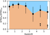 |
Fig. 9. Evolution of the fraction of the dust obscured SFRDIR as a function of redshift. The arrows show the lower limits obtained using the lower limits discussed in Sect. 4.3.1. The points at z < 4 are obtained using a compilation of the literature from Fig. 7. The points at z > 4 are obtained using the UVLF+GSMF combined measurements from Table 2. |
Since we used a sample of galaxies detected in FUV, we did not take into account the contribution from highly obscured and purely IR galaxies, which remains unknown at these redshifts, mainly due to the difficulties in detecting such galaxies. The low number counts of the most massive galaxies makes it difficult to make a statistical census. No sources with z > 5 were found by the deep ALMA observations of the Hubble Ultra-Deep Field (HUDF; Aravena et al. 2016; Dunlop et al. 2017; González-López et al. 2019). Only recently, a few sources with no optical or NIR counterparts were discovered with ALMA at z ∼ 4 and z ∼ 5 (Franco et al. 2018; Williams et al. 2019) and even z ∼ 6.9 (Strandet et al. 2017; Marrone et al. 2018). The largest sample up to date is assembled by Wang et al. (2019b). It contains 39 H-band dropouts at z > 3 observed with ALMA. Given their results, such galaxies could have an additional contribution of ∼11% to the total SFRD at z > 4. Since their sample is restricted to massive H-band dropouts, this is only a lower limit. The lower mass H-band dropouts could contribute to it significantly. Indeed, given the most recent results by Riechers et al. (2020), the dust obscured SFRD is log(SFRDIR M⊙ yr−1 Mpc−3) = −2.02 or 22% of the total SFRD (based on the space density of two sources detected by CO (J = 2→1) and not detected in the rest-frame UV and optical).
Another uncertainty comes from the fact that the conversion from the 158 μm flux to LIR in this work is based only on one point in the infrared SED. Therefore, our measurement of the total IR luminosity are dependent on the choice of the dust SED template. The infrared SED in high redshift galaxies is uncertain due to poorly constrained dust temperatures (Pavesi et al. 2016; Bouwens et al. 2016; Faisst et al. 2017, 2020). We tested a number of templates against the stacking of Herschel data and only used the ones, which are compatible with the Herschel stacks at redshift range of ALPINE (see appendix). The best fit of modified black body to these stacks gives the dust temperature Tdust = 41 ± 1 K at z ∼ 4.5 and Tdust = 43 ± 5 K at z ∼ 5.5 consistent with most recent measurements by Faisst et al. (2020; Tdust = 38 ± 8 at z ∼ 5.5). Although some uncertainties on the dust temperature and the rest-frame FIR part of the SED remain, we incorporate them into the uncertainty of our SFRD measurement by using an average conversion factor between the templates compatible with the stacks of Herschel data and taking into account the uncertainty of the conversion factor. Nevertheless, more observations are needed to better constrain the dust temperatures and SED of galaxies at z > 4.
5. Star-forming main sequence and sSFR evolution
The main sequence is the relation between the mass and SFR of star-forming galaxies. In Sect. 4.2, we derived the ⟨LIR⟩−M* relation. Here we use this relation to derive the main sequence. In each mass bin, we derive average SFR as ⟨SFR⟩=κFUV⟨L1600⟩+κIR⟨LIR⟩. The average ⟨L1600⟩ is computed from FUV absolute magnitudes, determined with the SED fitting, and the average ⟨LIR⟩ from stacks. As discussed in Sect. 3.2.2, we consider the results from the stacks as upper limits at masses below the completeness limits.
We derived the main sequence in the two redshifts bins: 4.4 < z < 4.7 and 5.1 < z < 5.8. We show the results in Fig. 10. The main sequence is well-defined and is in very good agreement with previous results from the literature (Santini et al. 2017; Tasca et al. 2015; Heinis et al. 2013; Khusanova et al. 2020). We fit the relation between SFR and mass with a power law. We find a slope α = 0.99 ± 0.08 at z ∼ 4.5. We find an excellent agreement with the Schreiber et al. (2015) parametrization of the main sequence evolution at z ∼ 4.5 based on Herschel data, even if we measure the SFRs at lower masses compared to Schreiber et al. (2015).
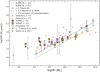 |
Fig. 10. Main sequence of star-forming galaxies at z ∼ 4.5 and z ∼ 5.5. The filled squares are the measurements of average SFR from stacks; the open symbols are results from the literature; the magenta and orange lines are the fits of the main sequence at z ∼ 4.5 and z ∼ 5.5 respectively; the cyan and green lines are the fits of the main sequence from the literature. The colored stars are the individual galaxies in ALPINE with FIR continuum detections at > 3σ. |
At z ∼ 5.5, we obtain a shallower slope α = 0.66 ± 0.21. The difference with the slope at z ∼ 4.5 is only 1.5σ, providing no evidence for an evolution of the slope between the two redshift bins. We note that at z ∼ 5.5, we could only provide FIR flux upper limits at lower masses due to the selection effects (see Sect. 3.2.2). Therefore, we only used three points to fit our data and the fit is subject to larger uncertainties. The slope of the main sequence found with Herschel data (Pearson et al. 2018) at the same redshift but at larger masses is steeper than found with ALPINE data, but still consistent with our data on stacks within the error bars.
In Fig. 10, we also plot the individual measurements for galaxies with continuum detections. As expected, most of them are above the main sequence since they represent the brightest galaxies with high SFRs. This confirms that it is necessary to use stacking to obtain unbiased measurements of the average SFR as a function of M* and fit the main sequence.
We measured the sSFR in the mass range 9.6 < log(M*/M⊙) < 9.8 as in Santini et al. (2017). The average sSFR is logsSFR(Gyr−1) = − 8.4 ± 0.18 and logsSFR(Gyr−1) = − 8.45 ± 0.16 at z ∼ 4.5 and z ∼ 5.5, respectively. We present a comparison with results from the literature in Fig. 11. We find good agreement within the error bars with the results from Khusanova et al. (2020) at z > 5 and with Herschel data at z ∼ 4 (Béthermin et al. 2015; Schreiber et al. 2015), although we note that the studies based on Herschel data probe only the high mass end (log(M*/M⊙) > 10.0) at z ∼ 4. The results are clearly against a steep increase in sSFR at z > 4 and even indicate a possible decrease in sSFR at high redshift. More observations at higher redshifts are necessary to explore this trend.
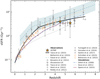 |
Fig. 11. SSFR evolution with redshift. Results of various observations and numerical simulations are shown (Dekel et al. 2009; Davé et al. 2011; Sparre et al. 2015). Gray symbols are based on FUV data (Bouwens et al. 2012; Khusanova et al. 2020; Tasca et al. 2015; Stark et al. 2013; Reddy et al. 2012; Fumagalli et al. 2014; González et al. 2014; Santini et al. 2017). Orange symbols are based on the rest-frame FIR data (Schreiber et al. 2015; Béthermin et al. 2015). The orange filled stars show this paper’s results. The solid line shows the fit to results by Tasca et al. (2015), the shaded area and the dashed line show the results coming from the observations of EW(Hα) in COSMOS (Faisst et al. 2016). |
If the growth of galaxies is regulated mainly by gas accretion through cold streams, the sSFR evolves as ∼(1 + z)2.25 (Dekel et al. 2009; Davé et al. 2011; Sparre et al. 2015). This is not the case at high redshifts. Therefore, another mechanism may play a role in the growth of galaxies, such as major and minor mergers (see e.g., Faisst et al. 2016). Another possible explanation could be the suppression of star formation by stronger stellar feedback at high redshifts and reduced star formation efficiency (see e.g., Weinmann et al. 2011). Future studies will place constraints on the role of different mechanisms regulating star formation and the growth of galaxies at high redshifts.
6. Conclusions
In this paper, we explored the SFRD, sSFR and main sequence evolution at z > 4 with ALPINE. Using the stacking technique, we constrained the average properties of galaxies even with low number of individual detections.
We provide the robust lower limits for infrared SFRD at z ∼ 4.5 and 5.5, which indicate that the dust plays an important role at high redshift and that dust build-up happens quite rapidly during and just after epoch of reionization. Based on extrapolated the density functions, we determine the total dust-hidden IR contribution to SFRD using either masses or FUV magnitudes as a proxy of IR luminosity. The results obtained using different proxies (see Table 2) agree with each other within the error bars. The results are  and
and  . They correspond to
  and
and  fractions of the star formation hidden by dust at z ∼ 4.5 and z ∼ 5.5 respectively. While at z < 4 the SFRDIR component dominates over the SFRDFUV, uncorr, at z > 4 their contributions are comparable. The SFRDIR approaches and possibly crosses the SFRDFUV, uncorr at z > 5 but this is yet to be confirmed with future observations.
Although our method by design does not include the contribution from ultra-dusty galaxies, our results agree with a number of independent measurements of the total SFRD at this redshift (based on IR luminosity function, [CII] luminosity function and gamma-ray bursts). Hence, we conclude that the major part of the SFRD can be traced by UV-selected galaxies.
The evolution of the total SFRD at redshifts higher than the peak of SFRD at z ∼ 2.5 may be shallower than previously measured. Further observations leading to reduced uncertainties are needed to confirm this conclusion.
We also provide robust measurements of SFRs of galaxies at z > 4 and use them to determine the main sequence at z ∼ 4.5 and z ∼ 5.5. We find that the observed main sequence is in good agreement with the previous results based on the rest-frame UV and optical data, as well as the IR data for the most massive galaxies. The main sequence has a slope α = 0.99 ± 0.08 at z ∼ 4.5 and α = 0.66 ± 0.21 at z ∼ 5.5, and no signs of turn-over at high masses. No significant evolution is observed from z ∼ 4.5 to z ∼ 5.5.
We use the SFR and mass measurements to determine the average sSFR of galaxies at z > 4. The results support a shallower or nonexistent sSFR evolution at high redshifts than predicted from models of cold gas accretion, or no evolution. Other mechanisms should play an important role in governing the growth of galaxies.
This is a commonly used value in the literature (e.g., Bouwens et al. 2015b; Madau & Dickinson 2014; Khusanova et al. 2020).
Acknowledgments
This paper is dedicated to the memory of Olivier Le Fèvre, PI of the ALPINE survey. This paper is based on data obtained with the ALMA Observatory, under Large Program 2017.1.00428.L. The Joint ALMA Observatory is operated by ESO, AUI/NRAO and NAOJ. ALMA is a partnership of ESO (representing its member states), NSF (USA) and NINS (Japan), together with NRC (Canada), MOST and ASIAA (Taiwan), and KASI (Republic of Korea), in cooperation with the Republic of Chile. This paper is based on data products from observations made with ESO Telescopes at the La Silla Paranal Observatory under ESO programme ID 179.A-2005 and on data products produced by TERAPIX and the Cambridge Astronomy Survey Unit on behalf of the UltraVISTA consortium. This work is based on data products made available at the CESAM data center, Laboratoire d’Astrophysique de Marseille, France. YK acknowledges the support by funding from the European Research Council Advanced Grant ERC–2010–AdG–268107–EARLY. AC, CG, FL, FP and MT acknowledge the support from grant PRIN MIUR 2017 - 20173ML3WW_001. GL acknowledges support from the European Research Council (ERC) under the European Union’s Horizon 2020 research and innovation programme (project CONCERTO, grant agreement No 788212) and from the Excellence Initiative of Aix-Marseille University-A*Midex, a French “Investissements d’Avenir” programme. D.R. acknowledges support from the National Science Foundation under grant numbers AST-1614213 and AST-1910107. D.R. also acknowledges support from the Alexander von Humboldt Foundation through a Humboldt Research Fellowship for Experienced Researchers. G.C.J. acknowledges ERC Advanced Grant 695671 “QUENCH” and support by the Science and Technology Facilities Council (STFC). S.T. acknowledges support from the ERC Consolidator Grant funding scheme (project ConTExt, grant number No. 648179). The Cosmic Dawn Center is funded by the Danish National Research Foundation under grant No. 140. R.A. acknowledges support from FONDECYT Regular Grant 1202007. This program is supported by the national program Cosmology and Galaxies from the CNRS in France.
References
- Álvarez-Márquez, J., Burgarella, D., Heinis, S., et al. 2016, A&A, 587, A122 [NASA ADS] [CrossRef] [EDP Sciences] [Google Scholar]
- Álvarez-Márquez, J., Burgarella, D., Buat, V., Ilbert, O., & Pérez-González, P. G. 2019, A&A, 630, A153 [NASA ADS] [CrossRef] [EDP Sciences] [Google Scholar]
- Aravena, M., Decarli, R., Walter, F., et al. 2016, ApJ, 833, 68 [NASA ADS] [CrossRef] [Google Scholar]
- Arnouts, S., Cristiani, S., Moscardini, L., et al. 1999, MNRAS, 310, 540 [NASA ADS] [CrossRef] [Google Scholar]
- Béthermin, M., Daddi, E., Magdis, G., et al. 2012, ApJ, 757, L23 [NASA ADS] [CrossRef] [Google Scholar]
- Béthermin, M., Daddi, E., Magdis, G., et al. 2015, A&A, 573, A113 [NASA ADS] [CrossRef] [EDP Sciences] [Google Scholar]
- Béthermin, M., Wu, H.-Y., Lagache, G., et al. 2017, A&A, 607, A89 [NASA ADS] [CrossRef] [EDP Sciences] [Google Scholar]
- Béthermin, M., Fudamoto, Y., Ginolfi, M., et al. 2020, A&A, 643, A2 [CrossRef] [EDP Sciences] [Google Scholar]
- Bolzonella, M., Miralles, J. M., & Pelló, R. 2000, A&A, 363, 476 [NASA ADS] [Google Scholar]
- Bouwens, R. J., Illingworth, G. D., Oesch, P. A., et al. 2012, ApJ, 754, 83 [NASA ADS] [CrossRef] [Google Scholar]
- Bouwens, R. J., Illingworth, G. D., Oesch, P. A., et al. 2015a, ApJ, 811, 140 [NASA ADS] [CrossRef] [Google Scholar]
- Bouwens, R. J., Illingworth, G. D., Oesch, P. A., et al. 2015b, ApJ, 803, 34 [Google Scholar]
- Bouwens, R. J., Aravena, M., Decarli, R., et al. 2016, ApJ, 833, 72 [NASA ADS] [CrossRef] [Google Scholar]
- Bowler, R. A. A., Dunlop, J. S., McLure, R. J., et al. 2015, MNRAS, 452, 1817 [NASA ADS] [CrossRef] [Google Scholar]
- Bowler, R. A. A., Bourne, N., Dunlop, J. S., McLure, R. J., & McLeod, D. J. 2018, MNRAS, 481, 1631 [NASA ADS] [CrossRef] [Google Scholar]
- Bruzual, G., & Charlot, S. 2003, MNRAS, 344, 1000 [NASA ADS] [CrossRef] [Google Scholar]
- Burgarella, D., Buat, V., Gruppioni, C., et al. 2013, A&A, 554, A70 [NASA ADS] [CrossRef] [EDP Sciences] [Google Scholar]
- Calura, F., Pozzi, F., Cresci, G., et al. 2017, MNRAS, 465, 54 [NASA ADS] [CrossRef] [Google Scholar]
- Capak, P. L., Carilli, C., Jones, G., et al. 2015, Nature, 522, 455 [NASA ADS] [CrossRef] [Google Scholar]
- Caputi, K. I., Michałowski, M. J., Krips, M., et al. 2014, ApJ, 788, 126 [NASA ADS] [CrossRef] [Google Scholar]
- Casey, C. M., Zavala, J. A., Spilker, J., et al. 2018, ApJ, 862, 77 [NASA ADS] [CrossRef] [Google Scholar]
- Chabrier, G. 2003, PASP, 115, 763 [Google Scholar]
- Cousin, M., Buat, V., Lagache, G., & Bethermin, M. 2019, A&A, 627, A132 [NASA ADS] [CrossRef] [EDP Sciences] [Google Scholar]
- Cucciati, O., Tresse, L., Ilbert, O., et al. 2012, A&A, 539, A31 [NASA ADS] [CrossRef] [EDP Sciences] [Google Scholar]
- Daddi, E., Dickinson, M., Morrison, G., et al. 2007, ApJ, 670, 156 [Google Scholar]
- Dahlen, T., Mobasher, B., Dickinson, M., et al. 2007, ApJ, 654, 172 [NASA ADS] [CrossRef] [Google Scholar]
- Davé, R., Oppenheimer, B. D., & Finlator, K. 2011, MNRAS, 415, 11 [NASA ADS] [CrossRef] [Google Scholar]
- Davidzon, I., Ilbert, O., Laigle, C., et al. 2017, A&A, 605, A70 [NASA ADS] [CrossRef] [EDP Sciences] [Google Scholar]
- Dayal, P., & Ferrara, A. 2018, Phys. Rep., 780, 1 [NASA ADS] [CrossRef] [Google Scholar]
- de Barros, S., Schaerer, D., & Stark, D. P. 2014, A&A, 563, A81 [NASA ADS] [CrossRef] [EDP Sciences] [Google Scholar]
- Dekel, A., Birnboim, Y., Engel, G., et al. 2009, Nature, 457, 451 [Google Scholar]
- De Rossi, M. E., Rieke, G. H., Shivaei, I., Bromm, V., & Lyu, J. 2018, ApJ, 869, 4 [Google Scholar]
- Dunlop, J. S., McLure, R. J., Biggs, A. D., et al. 2017, MNRAS, 466, 861 [Google Scholar]
- Faber, S. M., Phillips, A. C., Kibrick, R. I., et al. 2003, in The DEIMOS spectrograph for the Keck II Telescope: Integration and Testing, eds. M. Iye, & A. F. M. Moorwood, SPIE Conf. Ser., 4841, 1657 [Google Scholar]
- Faisst, A. L., Capak, P., Hsieh, B. C., et al. 2016, ApJ, 821, 122 [Google Scholar]
- Faisst, A. L., Capak, P. L., Yan, L., et al. 2017, ApJ, 847, 21 [NASA ADS] [CrossRef] [Google Scholar]
- Faisst, A. L., Schaerer, D., Lemaux, B. C., et al. 2020, ApJS, 247, 61 [NASA ADS] [CrossRef] [Google Scholar]
- Finkelstein, S. L., Ryan, Jr., R. E., Papovich, C., et al. 2015, ApJ, 810, 71 [NASA ADS] [CrossRef] [Google Scholar]
- Franco, M., Elbaz, D., Béthermin, M., et al. 2018, A&A, 620, A152 [NASA ADS] [CrossRef] [EDP Sciences] [Google Scholar]
- Fudamoto, Y., Oesch, P. A., Schinnerer, E., et al. 2017, MNRAS, 472, 483 [NASA ADS] [CrossRef] [Google Scholar]
- Fudamoto, Y., Oesch, P. A., Faisst, A., et al. 2020, A&A, 643, A4 [CrossRef] [EDP Sciences] [Google Scholar]
- Fujimoto, S., Silverman, J. D., Bethermin, M., et al. 2020, ApJ, 900, 1 [CrossRef] [Google Scholar]
- Fumagalli, M., Labbé, I., Patel, S. G., et al. 2014, ApJ, 796, 35 [NASA ADS] [CrossRef] [Google Scholar]
- Giacconi, R., Zirm, A., Wang, J., et al. 2002, ApJS, 139, 369 [NASA ADS] [CrossRef] [Google Scholar]
- González, V., Bouwens, R., Illingworth, G., et al. 2014, ApJ, 781, 34 [NASA ADS] [CrossRef] [Google Scholar]
- González-López, J., Decarli, R., Pavesi, R., et al. 2019, ApJ, 882, 139 [CrossRef] [Google Scholar]
- Grogin, N. A., Kocevski, D. D., Faber, S. M., et al. 2011, ApJS, 197, 35 [NASA ADS] [CrossRef] [Google Scholar]
- Gruppioni, C., & Pozzi, F. 2019, MNRAS, 483, 1993 [NASA ADS] [CrossRef] [Google Scholar]
- Gruppioni, C., Pozzi, F., Rodighiero, G., et al. 2013, MNRAS, 432, 23 [NASA ADS] [CrossRef] [Google Scholar]
- Gruppioni, C., Béthermin, M., Loiacono, F., et al. 2020, A&A, 643, A8 [CrossRef] [EDP Sciences] [Google Scholar]
- Hasinger, G., Capak, P., Salvato, M., et al. 2018, ApJ, 858, 77 [Google Scholar]
- Heinis, S., Buat, V., Béthermin, M., et al. 2013, MNRAS, 429, 1113 [Google Scholar]
- Ilbert, O., Arnouts, S., McCracken, H. J., et al. 2006, A&A, 457, 841 [NASA ADS] [CrossRef] [EDP Sciences] [Google Scholar]
- Kennicutt, R. C., Jr 1998, ApJ, 498, 541 [Google Scholar]
- Khusanova, Y., Le Fèvre, O., Cassata, P., et al. 2020, A&A, 634, A97 [CrossRef] [EDP Sciences] [Google Scholar]
- Kistler, M. D., Yüksel, H., Beacom, J. F., Hopkins, A. M., & Wyithe, J. S. B. 2009, ApJ, 705, L104 [NASA ADS] [CrossRef] [Google Scholar]
- Koekemoer, A. M., Faber, S. M., Ferguson, H. C., et al. 2011, ApJS, 197, 36 [NASA ADS] [CrossRef] [Google Scholar]
- Koprowski, M. P., Dunlop, J. S., Michałowski, M. J., et al. 2017, MNRAS, 471, 4155 [NASA ADS] [CrossRef] [Google Scholar]
- Laigle, C., McCracken, H. J., Ilbert, O., et al. 2016, ApJS, 224, 24 [NASA ADS] [CrossRef] [Google Scholar]
- Laporte, N., Ellis, R. S., Boone, F., et al. 2017, ApJ, 837, L21 [NASA ADS] [CrossRef] [Google Scholar]
- Le Fèvre, O., Tasca, L. A. M., Cassata, P., et al. 2015, A&A, 576, A79 [NASA ADS] [CrossRef] [EDP Sciences] [Google Scholar]
- Le Fèvre, O., Béthermin, M., Faisst, A., et al. 2020, A&A, 643, A1 [CrossRef] [EDP Sciences] [Google Scholar]
- Loiacono, F., Decarli, R., Gruppioni, C., et al. 2021, A&A, 646, A76 [EDP Sciences] [Google Scholar]
- Madau, P., & Dickinson, M. 2014, ARA&A, 52, 415 [NASA ADS] [CrossRef] [Google Scholar]
- Magdis, G. E., Daddi, E., Béthermin, M., et al. 2012, ApJ, 760, 6 [NASA ADS] [CrossRef] [Google Scholar]
- Magnelli, B., Elbaz, D., Chary, R. R., et al. 2011, A&A, 528, A35 [NASA ADS] [CrossRef] [EDP Sciences] [Google Scholar]
- Magnelli, B., Popesso, P., Berta, S., et al. 2013, A&A, 553, A132 [NASA ADS] [CrossRef] [EDP Sciences] [Google Scholar]
- Maniyar, A. S., Béthermin, M., & Lagache, G. 2018, A&A, 614, A39 [NASA ADS] [CrossRef] [EDP Sciences] [Google Scholar]
- Marrone, D. P., Spilker, J. S., Hayward, C. C., et al. 2018, Nature, 553, 51 [NASA ADS] [CrossRef] [Google Scholar]
- McMullin, J. P., Waters, B., Schiebel, D., Young, W., & Golap, K. 2007, in Astronomical Data Analysis Software and Systems XVI, eds. R. A. Shaw, F. Hill, & D. J. Bell, ASP Conf. Ser., 376, 127 [Google Scholar]
- Meurer, G. R., Heckman, T. M., & Calzetti, D. 1999, ApJ, 521, 64 [NASA ADS] [CrossRef] [Google Scholar]
- Neri, R., Downes, D., Cox, P., & Walter, F. 2014, A&A, 562, A35 [NASA ADS] [CrossRef] [EDP Sciences] [Google Scholar]
- Nguyen, H. T., Schulz, B., Levenson, L., et al. 2010, A&A, 518, L5 [NASA ADS] [CrossRef] [EDP Sciences] [Google Scholar]
- Noeske, K. G., Weiner, B. J., Faber, S. M., et al. 2007, ApJ, 660, L43 [Google Scholar]
- Ono, Y., Ouchi, M., Harikane, Y., et al. 2018, PASJ, 70, S10 [NASA ADS] [CrossRef] [Google Scholar]
- Pavesi, R., Riechers, D. A., Capak, P. L., et al. 2016, ApJ, 832, 151 [NASA ADS] [CrossRef] [Google Scholar]
- Pearson, W. J., Wang, L., Hurley, P. D., et al. 2018, A&A, 615, A146 [NASA ADS] [CrossRef] [EDP Sciences] [Google Scholar]
- Pelló, R., Hudelot, P., Laporte, N., et al. 2018, A&A, 620, A51 [CrossRef] [EDP Sciences] [Google Scholar]
- Planck Collaboration XXX. 2014, A&A, 571, A30 [NASA ADS] [CrossRef] [EDP Sciences] [Google Scholar]
- Reddy, N. A., & Steidel, C. C. 2009, ApJ, 692, 778 [NASA ADS] [CrossRef] [Google Scholar]
- Reddy, N. A., Pettini, M., Steidel, C. C., et al. 2012, ApJ, 754, 25 [NASA ADS] [CrossRef] [Google Scholar]
- Riechers, D. A., Bradford, C. M., Clements, D. L., et al. 2013, Nature, 496, 329 [Google Scholar]
- Riechers, D. A., Hodge, J. A., Pavesi, R., et al. 2020, ApJ, 895, 81 [Google Scholar]
- Robertson, B. E., Ellis, R. S., Furlanetto, S. R., & Dunlop, J. S. 2015, ApJ, 802, L19 [Google Scholar]
- Rowan-Robinson, M., Oliver, S., Wang, L., et al. 2016, MNRAS, 461, 1100 [NASA ADS] [CrossRef] [Google Scholar]
- Salmon, B., Papovich, C., Finkelstein, S. L., et al. 2015, ApJ, 799, 183 [NASA ADS] [CrossRef] [Google Scholar]
- Sanders, D. B., Mazzarella, J. M., Kim, D. C., Surace, J. A., & Soifer, B. T. 2003, AJ, 126, 1607 [Google Scholar]
- Santini, P., Fontana, A., Castellano, M., et al. 2017, ApJ, 847, 76 [NASA ADS] [CrossRef] [Google Scholar]
- Schaerer, D., Ginolfi, M., Bethermin, M., et al. 2020, A&A, 643, A3 [CrossRef] [EDP Sciences] [Google Scholar]
- Schenker, M. A., Robertson, B. E., Ellis, R. S., et al. 2013, ApJ, 768, 196 [NASA ADS] [CrossRef] [Google Scholar]
- Schreiber, C., Pannella, M., Elbaz, D., et al. 2015, A&A, 575, A74 [NASA ADS] [CrossRef] [EDP Sciences] [Google Scholar]
- Schreiber, C., Elbaz, D., Pannella, M., et al. 2018, A&A, 609, A30 [NASA ADS] [CrossRef] [EDP Sciences] [Google Scholar]
- Scoville, N., Aussel, H., Brusa, M., et al. 2007, ApJS, 172, 1 [NASA ADS] [CrossRef] [Google Scholar]
- Skelton, R. E., Whitaker, K. E., Momcheva, I. G., et al. 2014, ApJS, 214, 24 [Google Scholar]
- Song, M., Finkelstein, S. L., Ashby, M. L. N., et al. 2016, ApJ, 825, 5 [NASA ADS] [CrossRef] [Google Scholar]
- Sparre, M., Hayward, C. C., Springel, V., et al. 2015, MNRAS, 447, 3548 [Google Scholar]
- Speagle, J. S., Steinhardt, C. L., Capak, P. L., & Silverman, J. D. 2014, ApJS, 214, 15 [NASA ADS] [CrossRef] [Google Scholar]
- Stark, D. P., Schenker, M. A., Ellis, R., et al. 2013, ApJ, 763, 129 [NASA ADS] [CrossRef] [Google Scholar]
- Strandet, M. L., Weiss, A., De Breuck, C., et al. 2017, ApJ, 842, L15 [Google Scholar]
- Takeuchi, T. T., Yoshikawa, K., & Ishii, T. T. 2003, ApJ, 587, L89 [NASA ADS] [CrossRef] [Google Scholar]
- Tamura, Y., Mawatari, K., Hashimoto, T., et al. 2019, ApJ, 874, 27 [NASA ADS] [CrossRef] [Google Scholar]
- Tasca, L. A. M., Le Fèvre, O., Hathi, N. P., et al. 2015, A&A, 581, A54 [NASA ADS] [CrossRef] [EDP Sciences] [Google Scholar]
- Tasca, L. A. M., Le Fèvre, O., Ribeiro, B., et al. 2017, A&A, 600, A110 [NASA ADS] [CrossRef] [EDP Sciences] [Google Scholar]
- Tomczak, A. R., Quadri, R. F., Tran, K.-V. H., et al. 2016, ApJ, 817, 118 [NASA ADS] [CrossRef] [Google Scholar]
- Wang, L., Pearson, W. J., Cowley, W., et al. 2019a, A&A, 624, A98 [CrossRef] [EDP Sciences] [Google Scholar]
- Wang, T., Schreiber, C., Elbaz, D., et al. 2019b, Nature, 572, 211 [Google Scholar]
- Weinmann, S. M., Neistein, E., & Dekel, A. 2011, MNRAS, 417, 2737 [NASA ADS] [CrossRef] [Google Scholar]
- Whitaker, K. E., van Dokkum, P. G., Brammer, G., & Franx, M. 2012, ApJ, 754, L29 [NASA ADS] [CrossRef] [Google Scholar]
- Whitaker, K. E., Franx, M., Leja, J., et al. 2014, ApJ, 795, 104 [NASA ADS] [CrossRef] [MathSciNet] [Google Scholar]
- Williams, C. C., Labbe, I., Spilker, J., et al. 2019, ApJ, 884, 154 [CrossRef] [Google Scholar]
- Wright, A. H., Driver, S. P., & Robotham, A. S. G. 2018, MNRAS, 480, 3491 [NASA ADS] [CrossRef] [Google Scholar]
- Yan, L., Sajina, A., Loiacono, F., et al. 2020, ApJ, 905, 147 [Google Scholar]
- Zavala, J. A., Casey, C. M., da Cunha, E., et al. 2018, ApJ, 869, 71 [Google Scholar]
Appendix A: Conversion of FIR flux to IR luminosity
To convert the rest-frame 158 μm flux to IR luminosity, we scaled our flux measurement to the dust SED template and then integrated it from 8 to 1000 μm. Since we used stacks of galaxies, which are not at the same redshift, we used the mean redshift of galaxies in stacks for that conversion. Since we only obtain a measurement of one point in SED, our conversion to IR luminosity depends on dust SED templates.
There are numerous dust SED templates available in the literature (e.g., Magdis et al. 2012; Béthermin et al. 2017; Álvarez-Márquez et al. 2016; Casey et al. 2018; Schreiber et al. 2018; De Rossi et al. 2018; Álvarez-Márquez et al. 2019). Some of them were already discussed and tested by Béthermin et al. (2020). Béthermin et al. (2020) made stacks of Herschel data for galaxies at z > 4 selected via photometric redshifts. They then compared the SED templates to these stacks. The fit with the modified black body model corresponds to the average dust temperature Td = 41 ± 1 K at z ∼ 4.5 and Td = 43 ± 5 K at z ∼ 5.5 for galaxies with SFR > 10 M⊙ yr−1. The SFR limit is defined by completeness of the sample. It is not possible to test whether the dust temperature is lower for fainter galaxies, due to this limitation. However, the uncertainty on the choice of the template naturally includes the uncertainty on the dust temperature. When we convert the IR luminosity in each bin of MFUV or M* to SFR, we assume that we do not know the exact dust temperature typical for this MFUV or M* and that the uncertainty on the conversion factor includes the uncertainty on the dust temperature.
We defined the conversion factor ftemp for each template and the χ2 from comparison to Herschel stacks at both redshifts (see Table A.1). The conversion factor is defined as ftemp = νLν = 158μm/LIR. We discarded the templates with reduced χ2 > 1.5 in at least one of the redshift bins (see Fig. A.3). We defined the mean conversion factors from the remaining templates ⟨ftemp, z ∼ 4.5⟩ = 0.13 ± 0.02 and ⟨ftemp, z ∼ 5.5⟩ = 0.12 ± 0.03 for redshift bins 4 < z < 5 and 5 < z < 6 respectively. These are the values we used to convert the monochromatic flux to the IR luminosity and propagate their uncertainties into our SFRD measurements.
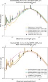 |
Fig. A.1. Comparison of the chosen dust SED templates with the stacks of Herschel data at 4 < z < 5. The black symbols are stacked Herschel data and the solid lines are templates from the literature. |
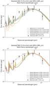 |
Fig. A.2. Comparison of the chosen dust SED templates with the stacks of Herschel data at 5 < z < 6. The black symbols are stacked Herschel data and the solid lines are templates from the literature. |
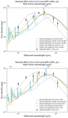 |
Fig. A.3. Comparison of the discarded dust SED templates with the stacks of Herschel data at. The black symbols are stacked Herschel data and the dashed lines are templates from the literature. |
Dust SED templates, conversion factors ftemp, and SFRDIR corresponding to templates from the literature.
We note that although the De Rossi et al. (2018) template passes our χ2 criteria, it goes above the upper limits in redshift bin 4 < z < 5, but is perfectly consistent at 5 < z < 6. Therefore, we used this template only for 5 < z < 6 redshift bin.
All Tables
Dust SED templates, conversion factors ftemp, and SFRDIR corresponding to templates from the literature.
All Figures
|
Fig. 1. Comparison of injected and recovered fluxes from stacking. The vertical dashed lines correspond to 16th, 50th and 84th percentiles of the distribution (−1.08, −0.02, 1.03). |
| In the text | |
|
Fig. 2. Illustration of the method used to determine the SFRDIR. Left panel: steps performed. Right panel: arbitrary proxy density function (UVLF or GSMF) and a power law relation between the property used as a proxy and the FIR flux. The black squares represent measured values and the solid line the fit with uncertainties represented by a shaded region. The vertical shaded regions show the proxy range, in which the data is available for both the power law relation derived from ALPINE and the proxy density function. |
| In the text | |
|
Fig. 3. Stellar mass versus FUV magnitude. The black circles are ALPINE targets as measured by Faisst et al. (2020). The open squares are measurements from Salmon et al. (2015). The solid blue line is the fit to the measurements by Salmon et al. (2015) and the shaded areas are 1σ uncertainties. The vertical dotted line shows the FUV luminosity cut used in selecting galaxies. The vertical dotted lines show the mass limits below which the flux measurements are considered to be upper limits. Left panel: z ∼ 4.5 redshift bin and right panel: z ∼ 5.5 bin. |
| In the text | |
|
Fig. 4. Average infrared luminosity versus proxy (stellar mass as a proxy on the left panel and FUV magnitude on the right). The green squares and blue circles are the average IR luminosities on the stacks at z ∼ 4.5 and z ∼ 5.5, respectively. The black error bars show the population variance (σpop), the colored error bars show the photometric noise (σphot, see Eq. (1), Sect. 3.1). The open squares are the flux measurements on stacks below mass limit Mlim. The stars are the results on stacks excluding the galaxies with signs of possible contamination by a close companion. The green and blue dashed lines are the best fits of the relation and the thin lines of corresponding color are the MCMC chain realizations of the fit. Top panels: S/N on each stack. |
| In the text | |
|
Fig. 5. Probability distribution of the SFRDIR at redshift z ∼ 4.5. All distributions are derived with the same relations between the stellar mass (bottom panels) and FUV magnitudes (top panels). The minimum is derived in the observed by ALPINE range of stellar masses and FUV magnitudes and is shown on the left panels. The SFRDs from extrapolated relation are shown on the right panels. Different colors correspond to different GSMFs and UVLFs (Bouwens et al. 2015b; Finkelstein et al. 2015; Ono et al. 2018; Davidzon et al. 2017; Song et al. 2016; Wright et al. 2018). |
| In the text | |
|
Fig. 6. Same as Fig. 5, but at redshift z ∼ 5.5. The UVLFs and GSMF are taken from Bouwens et al. (2015b), Pelló et al. (2018), Khusanova et al. (2020), Davidzon et al. (2017), Song et al. (2016), Wright et al. (2018). |
| In the text | |
|
Fig. 7. Evolution of the total SFRD (Eq. (2)) with redshift. The red symbols are the total SFRDs, derived in this paper. Small offsets of ±0.08 are applied to their redshift for clarity. The triangles are the lower limits for SFRDIR derived in Sect. 4.3.1. The blue symbols are dust-corrected SFRD derived from the FUV data (Cucciati et al. 2012; Dahlen et al. 2007; Reddy & Steidel 2009; Bouwens et al. 2012, 2015b; Schenker et al. 2013; Pelló et al. 2018; Khusanova et al. 2020), orange symbols are derived from reradiated dust emission from forming stars as measured from the IR (Magnelli et al. 2013; Gruppioni et al. 2013, 2020; Rowan-Robinson et al. 2016; Koprowski et al. 2017; Wang et al. 2019a; Riechers et al. 2020). The magenta points are from other SFR tracers: [CII] luminosity function based on the ALPINE field sample of Loiacono et al. (2021) and number counts of γ-ray bursts (Kistler et al. 2009). The dotted line is the fit of SFRD evolution from Madau & Dickinson (2014). |
| In the text | |
|
Fig. 8. Evolution of SFRDIR and SFRDFUV, uncorr with redshift. The red symbols are the SFRDIR, derived in this paper. Small offsets of ±0.08 are applied to their redshift for clarity. The triangles are the lower limits for SFRDIR derived in Sect. 4.3.1. The blue symbols are SFRDFUV, uncorr derived from the FUV data (Cucciati et al. 2012; Dahlen et al. 2007; Reddy & Steidel 2009; Bouwens et al. 2012, 2015b; Schenker et al. 2013; Pelló et al. 2018; Khusanova et al. 2020), orange symbols are SFRDIR from Magnelli et al. (2013), Gruppioni et al. (2013, 2020), Rowan-Robinson et al. (2016), Koprowski et al. (2017), Wang et al. (2019a) and Riechers et al. (2020). Orange lines are the fits of SFRDIR evolution from Koprowski et al. (2017) and Maniyar et al. (2018). |
| In the text | |
|
Fig. 9. Evolution of the fraction of the dust obscured SFRDIR as a function of redshift. The arrows show the lower limits obtained using the lower limits discussed in Sect. 4.3.1. The points at z < 4 are obtained using a compilation of the literature from Fig. 7. The points at z > 4 are obtained using the UVLF+GSMF combined measurements from Table 2. |
| In the text | |
|
Fig. 10. Main sequence of star-forming galaxies at z ∼ 4.5 and z ∼ 5.5. The filled squares are the measurements of average SFR from stacks; the open symbols are results from the literature; the magenta and orange lines are the fits of the main sequence at z ∼ 4.5 and z ∼ 5.5 respectively; the cyan and green lines are the fits of the main sequence from the literature. The colored stars are the individual galaxies in ALPINE with FIR continuum detections at > 3σ. |
| In the text | |
|
Fig. 11. SSFR evolution with redshift. Results of various observations and numerical simulations are shown (Dekel et al. 2009; Davé et al. 2011; Sparre et al. 2015). Gray symbols are based on FUV data (Bouwens et al. 2012; Khusanova et al. 2020; Tasca et al. 2015; Stark et al. 2013; Reddy et al. 2012; Fumagalli et al. 2014; González et al. 2014; Santini et al. 2017). Orange symbols are based on the rest-frame FIR data (Schreiber et al. 2015; Béthermin et al. 2015). The orange filled stars show this paper’s results. The solid line shows the fit to results by Tasca et al. (2015), the shaded area and the dashed line show the results coming from the observations of EW(Hα) in COSMOS (Faisst et al. 2016). |
| In the text | |
|
Fig. A.1. Comparison of the chosen dust SED templates with the stacks of Herschel data at 4 < z < 5. The black symbols are stacked Herschel data and the solid lines are templates from the literature. |
| In the text | |
|
Fig. A.2. Comparison of the chosen dust SED templates with the stacks of Herschel data at 5 < z < 6. The black symbols are stacked Herschel data and the solid lines are templates from the literature. |
| In the text | |
|
Fig. A.3. Comparison of the discarded dust SED templates with the stacks of Herschel data at. The black symbols are stacked Herschel data and the dashed lines are templates from the literature. |
| In the text | |
Current usage metrics show cumulative count of Article Views (full-text article views including HTML views, PDF and ePub downloads, according to the available data) and Abstracts Views on Vision4Press platform.
Data correspond to usage on the plateform after 2015. The current usage metrics is available 48-96 hours after online publication and is updated daily on week days.
Initial download of the metrics may take a while.