| Issue |
A&A
Volume 648, April 2021
|
|
|---|---|---|
| Article Number | A49 | |
| Number of page(s) | 34 | |
| Section | Planets and planetary systems | |
| DOI | https://doi.org/10.1051/0004-6361/202040125 | |
| Published online | 09 April 2021 | |
Molecular composition of comet 46P/Wirtanen from millimetre-wave spectroscopy★,★★
1
LESIA, Observatoire de Paris, PSL Research University, CNRS, Sorbonne Université, Université de Paris,
5 place Jules Janssen,
92195
Meudon,
France
e-mail: nicolas.biver@obspm.fr
2
IRAM, 300 rue de la Piscine,
38406
Saint Martin d’Hères,
France
3
Jet Propulsion Laboratory, California Institute of Technology,
4800 Oak Grove Drive,
Pasadena,
CA
91109,
USA
4
Solar System Exploration Division,
Astrochemistry Laboratory Code 691, NASA-GSFC,
Greenbelt,
MD 20771,
USA
5
Department of Physics, Catholic University of America,
Washington,
DC 20064,
USA
6
Department of Physics, American University,
Washington,
DC,
USA
7
Johns Hopkins University Applied Physics Laboratory,
11100 Johns Hopkins Rd.,
Laurel,
MD 20723,
USA
8
Solar System Exploration Division,
Planetary System Laboratory Code 693, NASA-GSFC,
Greenbelt,
MD 20771,
USA
Received:
14
December
2020
Accepted:
10
February
2021
We present the results of a molecular survey of comet 46P/Wirtanen undertaken with the IRAM 30-m and NOEMA radio telescopes in December 2018. Observations at IRAM 30-m during the 12–18 December period comprise a 2 mm spectral survey covering 25 GHz and a 1 mm survey covering 62 GHz. The gas outflow velocity and kinetic temperature have been accurately constrained by the observations. We derive abundances of 11 molecules, some being identified remotely for the first time in a Jupiter-family comet, including complex organic molecules such as formamide, ethylene glycol, acetaldehyde, or ethanol. Sensitive upper limits on the abundances of 24 other molecules are obtained. The comet is found to be relatively rich in methanol (3.4% relative to water), but relatively depleted in CO, CS, HNC, HNCO, and HCOOH.
Key words: comets: general / comets: individual: 46P/Wirtanen / radio lines: planetary systems / submillimeter: planetary systems
The radio spectra are only available at the CDS via anonymous ftp to cdsarc.u-strasbg.fr (130.79.128.5) or via http://cdsarc.u-strasbg.fr/viz-bin/cat/J/A+A/648/A49
© N. Biver et al. 2021
 Open Access article, published by EDP Sciences, under the terms of the Creative Commons Attribution License (https://creativecommons.org/licenses/by/4.0), which permits unrestricted use, distribution, and reproduction in any medium, provided the original work is properly cited.
1 Introduction
Comets are the most pristine remnants of the formation of the Solar System 4.6 billion years ago. They sample some of the oldest and most primitive material in the Solar System, including ices, and are thus our best window to the volatile composition of the solar proto-planetary disk. Comets may also have played a role in the delivery of water and organic material to the early Earth (see Hartogh et al. 2011, and references therein). The latest simulations of the early Solar System’s evolution (Brasser & Morbidelli 2013; O’Brien et al. 2014) suggest a more complex scenario. On the one hand, ice-rich bodies formed beyond Jupiter may have been implanted in the outer asteroid belt and participated in the supply of water to the Earth, or, on the other hand, current comets coming from either the Oort Cloud or the scattered disk of the Kuiper belt may have formed in the same trans-Neptunian region, sampling the same diversity of formation conditions. Understanding the diversity in composition and isotopic ratios of comet material is thus essential in order to assess such scenarios (Altwegg & Bockelée-Morvan 2003; Bockelée-Morvan et al. 2015).
Comet 46P/Wirtanen is a Jupiter-family comet (JFC) orbiting the Sun in 5.4 yr on a low inclination (11.7°) orbit. It reached perihelion on 12.9 Dec 2018 UT at 1.055 au from the Sun. It made its closest ever approach to the Earth on 16 December at only 0.078 au. It remained within 0.1 au from the Earth for 3 weeks, and this provided one of the best opportunities for ground-based investigation of a Jupiter-family comet. Such an orbit makes it well suited for spacecraft exploration, and 46P was the initial target of the ESA Rosetta mission, until it was replaced by comet 67P/Churyumov-Gerasimenko.
We observed comet 46P with the Institut de RadioAstronomie Millimétrique (IRAM) 30-m telescope between 11.8 and 18.1 Dec 2018 UT, on 21.0, 25.2 and 25.8 Dec UT with the NOrthern Extended Millimeter Array (NOEMA) and with the Nançay radio telescope. In this paper, we report the detection of a dozen of molecules and significant upper limits for nearly two dozen additional ones, obtained in single-dish mode. Sect. 2 presents the observations and Sect. 3 presents the spectra of the detected molecules. The information extracted from the observations to analyse the data and compute production rates is provided in Sect. 4. In Sect. 5, we discuss the uncertainties related to the molecular lifetimes and present the retrieved production rates and abundances or upper limits, which are discussed and compared to other comets in Sect. 6.
2 Observations of comet 46P/Wirtanen
Comet 46P/Wirtanen was observed around the time of its closest approach to the Sun and the Earth with several radio facilities (Nançay, IRAM, NOEMA, the Atacama Large Millimeter/ submillimeter Array (ALMA) and the Stratospheric Observatory for Infrared Astronomy (SOFIA)). We focus here on single-dish measurements obtained with the IRAM and NOEMA millimetre radio telescopes. The OH radical was observed with the Nançay radio telescope between 1 September 2018 and 28 February 2019, and observations covering the period of interest are presented in Sect. 4.3. ALMA data will be presented in a future paper (Biver et al., in prep.), and SOFIA results are reported in Lis et al. (2019).
Log of millimetre observations.
2.1 Observations with the IRAM 30-m
Comet 46P/Wirtanen was the target of the observing proposal 112-18 scheduled at the IRAM 30-m telescope between 11 and 18 December 2018. Weather conditions were very good to average, with precipitable water vapour (pwv) in the 0.4–8 mm range (Table 1). The worst (cloudy) conditions were at the end of the 12 Dec. run (pwv up to 8 mm on 13.1 Dec. UT) followed by a day without observations. Around 17.0 Dec. UT, very low opacity (~ 0.5 mm pwv) enabled observations around 183 GHz. Observations were obtained in wobbler switching mode with the secondary (wobbling) mirror alternating pointing between the ON and OFF positions separated by 180′′ every 2 s.
Comet 46P was tracked using the latest JPL#181/111 orbital elements, and following orbit solutions, to compute a position in real time with IRAM New Control System (NCS) software. Unfortunately, the proximity of the comet to the Earth (0.08 au) challenged the accuracy of the NCS software and resulted in an ephemeris error of the order of 24′′ in RA and 10′′ in declination, changing by a few arc-seconds from day to day. These initial offsets were estimated from a map of HCN(3–2) on the first day and used for the following days. The exact ephemeris error was computed afterwards from the comparison of the output of the NCS ephemeris and the JPL#181/16 ephemeris solution. The pointing was regularly checked on bright pointing sources (rms < 1′′). Uranus pointing data were also used to check the beam efficiency of the antenna, and the beam size, which follows the formula θ ~ 2460∕ν[GHz] in ′′. Coarse maps obtained on HCN (e.g. Fig. 1), CH3OH, and H2S show an average residual offset between the maximum brightness and the target position of (− 1′′, −1′′) that was used to compute the final average radial offsets given in Table A.1.
We used the EMIR (Carter et al. 2012) 2 and 1 mm band receivers in 2SB mode connected to the FTS and VESPA high-resolution spectrometers (see Table 1).
2.2 Observations conducted with NOEMA
Comet 46P/Wirtanen was also observed with the NOEMA interferometer on 21.0, 25.2, and 25.8 Dec. UT, as part of the proposal W18AB, at 3, 1, and 2 mm wavelengths. Here, we only report the ON–OFF position switching data obtained during part of these observationsfor the zero-spacing information needed to analyse interferometric data. The versatile Polyfix correlator was used to target some dedicated molecular lines in addition to the continuum, and here we analyse the spectra of the lines detected in this autocorrelation mode. The frequency coverage and total integration time (adding up the 8–10 antennas) is provided in Table 1.
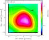 |
Fig. 1 Map of HCN(3-2) line-integrated intensity in comet 46P/Wirtanen on 17.82 Dec. 2018. Offsets are relative to JPL#181/16 position and corrected for estimated pointing errors. The direction of the Sun is indicated by the arrow in the upper right. Contours are drawn every 0.225 Kkm s−1. |
3 Spectra and line intensities
A sample of IRAM spectra at 1 and 2 mm is shown in Figs. 2–3. These are averages over the six nights of observations, sampling most of the detected species in the two wavelength domains. For some species, the spectra are the weighted averages of several lines to increase the signal-to-noise ratio (S/N), with a weight inferred from to the noise of individual spectra. Spectra are aligned on the velocity scale to provide information on the line shape. However, the computation of production rate is not based on the average line intensity but on the weighted average of the production rates derived from each individual line (the weight is larger for the lines expected to be the strongest). Full spectra are shown in Figs. B.1 and C.1. Examples of CH3 OH lines used to derive the gas temperature are also shown in Figs. 4 and 5. Only spectra obtained at pointing offset <3′′ are shown.
Line intensities are given in Tables 2 and A.1, including values obtained at the offset position (radial averages). Table 2 focuses on species for which several individual lines, eventually grouped by series probing levels of similar energy, were averaged. We also provide, for other molecules, the average intensity or upper limits for non-detections. Where individual lines are not detected, we selected the strongest transitions that are expected to have a similar intensity for the averages (within a factor of 2–3).
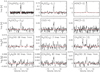 |
Fig. 2 Molecular lines observed in comet 46P/Wirtanen between 11.9 and 18.1 Dec. 2018. For some complex organics, we averaged several lines between 210 and 272 GHz (1 mm wavelength band). The vertical scale is the main beam brightness temperatureand the horizontal scale is the Doppler velocity in the comet rest frame. |
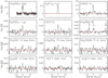 |
Fig. 3 Molecular lines observed in comet 46P/Wirtanen between 11.9 and 18.1 Dec 2018 in the 2 mm band, except for HC3 N and OCS, for which we show the weighted average of five lines expected in the 1 mm band. For some complex organics, we averaged several lines between 147 and 170 GHz (2 mm wavelength). The vertical scale is the main beam brightness temperatureand the horizontal scale is the Doppler velocity in the comet rest frame. |
4 Data analysis
4.1 Expansion velocity and outgassing pattern
We used the line profiles with the highest S/N and those of CH3 OH obtained with the high spectral resolution (40 kHz) VESPA spectrometer (e.g. Figs. 2 and 3). As lines are often double-peaked or asymmetric, we fitted two Gaussians, one to each of the blueshifted (v < 0) and redshifted (v > 0) peaks. The velocity of the channel at half the maximum intensity (VHM) of these fits provides a good estimate of the expansion velocity, towards the observer for the negative-velocity (blueshifted) side and for the gas moving in the opposite direction for the positive-velocity (redshifted) side. We found the following for the VHM:
-
V HM(HCN(3-2)) = − 0.87 ± 0.01 and + 0.48 ± 0.01 km s−1;
-
V HM(H2S(110−101)) = − 0.86 ± 0.02 and +0.47 ± 0.02 km s−1;
-
V HM(CH3OH(six lines 165–266 GHz)) = − 0.83 ± 0.01 and +0.42 ± 0.02 km s−1.
On average, thissuggests an expansion velocity of 0.85 km s−1 on the observer or day side and 0.45 km s−1 on the anti-observer or night side. For HCN, for example, if we model an hemispheric day side outgassing at 0.85 km s−1 and outgassing at 0.45 km s−1 separately in the other hemisphere, to retrieve the observed Doppler shift (− 0.17 km s−1) we need a production rate ratio Qday∕Qnight = 2.3. The corresponding total production rate (Qday + Qnight) is only 2 ± 2% higher than the value found when assuming isotropic outgassing at a velocity of 0.65 km s−1. Since modelling an asymmetric outgassing pattern does not significantly change the retrieved total outgassing rates, to compute the production rates we assumed isotropic outgassing at the mean velocity, that is, 0.65 km s−1.
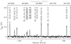 |
Fig. 4 Series of methanol lines around 242 GHz observed in comet 46P/Wirtanen between 12.0 and 17.9 Dec. 2018. The vertical scale is the main beam brightness temperature, and the horizontal scale is the Doppler velocity in the comet rest frame and frequency in the comet frame on the upper scale. |
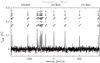 |
Fig. 5 Series of methanol lines around 252 GHz observed in comet 46P/Wirtanen between 11.8 and 17.8 Dec. 2018. The vertical scale is the main beam brightness temperature, and the horizontal scale is the Doppler velocity in the comet rest frame and frequency in the comet frame on the upper scale. |
4.2 Gas temperature
Many series of lines (especially of methanol but also CH3 CN) were detected at several times during the observations. Examples of these data as well as rotational diagrams are shown in Figs. 2–5 and Figs. 6–8, respectively. Inferred rotational temperatures Trot are given in Table 3. For each of these measurements, we retrieve constraints on the gas temperature, Tgas , needed to obtain such rotational temperatures. For some series of transitions, such as the CH3 OH lines at 165 or 252 GHz, Tgas is close and proportional to Trot. For CH3 CN, our code (e.g. Biver et al. 1999, 2006) predicts T = Trot, but for species like H2S there is a large difference due to rapid radiative decay of the levels’ population in the inner coma. The evolution of Trot with nucleocentric distance (400–1500 km) does not show any trend (Fig. 9). A decrease of Trot (CH3OH 242 GHz) and a smaller one for Trot (CH3OH 252 GHz) is expected and compatible with observations. In Fig. 10, we also plotted the retrieved Tgas temperatures for the daily measurements from Table 3. The decrease of the gas temperature with radial distance from the nucleus would likely explain the systematically higher Tgas deduced from the 252 GHz lines. There might also be a longer week-long trend, but the adopted Tgas= 60 K value is within ~ 2 −σ of all values in Table 3. A ± 10 K variation of the gas temperature will not impact the production rates by more than ± 5–10% (using several lines to retrieve the production rate of a molecule decreases the impact).
We also performed the rotation diagram analysis independently for the blueshifted and red-shifted components of the lines. We derive the corresponding Earth (~day) side and opposite (~ night) rotational temperature for the average of the CH3OH lines at 165 or 252 GHz. There is no day/night asymmetry based on the 165 GHz lines (beam ≈ 900 km), but the 252 GHz lines that probe the gas closer (<600 km) to the nucleus do show a higher night-gas temperature (Table 3), an effect observed in situ in the coma of comet 67P (Biver & Bockelée-Morvan 2019) that can be explained as a less efficient adiabatic cooling on the night side where the outgassing rate is lower.
Infrared observations (Bonev et al. 2020; Khan et al. 2020) that probed the coma closer to the nucleus (within 50 km) found higher gas temperatures (80–90 K) decreasing slightly with projected distance to the nucleus (100–200 km, Bonev et al. 2020)down to values closer to ours (Figs. 9 and 10). This is often the case when comparing ground-based radio and infrared measurements, indicative of some degree of adiabatic cooling between the distances probed by the two techniques.
4.3 Reference water production rate
We used the water production rates derived from the observation of the H O line with the SOFIA airborne observatory – assuming 16 O/18O = 500 (Lis et al. 2019). These observations were obtained with a somewhat larger beam (50′′ ; although smaller than the Nançay or SWAN fields of view) but cover the same period (14–20 December 2018) and were analysed with the same numerical codes. The average value of
  molec s−1 was used for the computation of excitation conditions (collisions) and relative abundances. Water production rates measured from infrared observations at the same time (Bonev et al. 2020) yield about the same value. The measurements of Combi et al. (2020) of Lyman-α emission with the SOHO/SWAN experiment do not cover the period of closest approach to the Earth, but derived
  molec s−1 on 10.9 Dec 2018.
We also tried to detect directly the H2 O(313−220) line at 183.3 GHz (Fig. B.1) during a period of very good weather at IRAM, but we could not integrate long enough and the weather proved too marginal for this observation. In addition the calibration uncertainty is likely large at this frequency (± 50% probably): on the one hand the HCN(2-1) line in the same band and a methanol line yield a correct production rate, but on the other hand the water maser line observed in Orion spectra acquired for calibration purposes is somewhat stronger than expected. We obtain a 3 − σ upper limit  molec s−1, which is a factor ~6 times higher than the other measured values. This has been derived using the same approach as for all other molecules as detailed in the next section. Line opacity is taken into account both for excitation (as detailed in e.g. Biver et al. 2007) and radiative transfer.
Line intensities from IRAM observations: multi-line averages.
4.4 Production rates of OH from Nançay observations
The OH 18-cm lines were observed in 46P with the Nançay radio telescope from 12 to 20 December, thanks to a small positive inversion of the OH maser. The OH inversion peaked on 16 December when the heliocentric radial velocity was 1.0 km s−1, at 0.040 according to Despois et al. (1981) or at 0.099 based on Schleicher & A’Hearn (1988).
The time-averaged spectrum is shown in Fig. 11. An emission line is definitely detected. The corresponding OH production rate is 1.7 ± 0.4 × 1028 molec s−1 using our nominal model with quenching (see Crovisier et al. 2002) and the inversion of Despois et al. For the inversion of Schleicher & A’Hearn, the production rate is lowered to 0.7 ± 0.2 × 1028 molec s−1. These values, although imprecise due to the uncertainty on the OH excitation, are in line with the other measurements of the water production rate.
The OH line is observed to be unusually narrow with a full width at half maximum (FWHM) of 1.1 ± 0.2 km s−1. This is comparable to the line widths observed for parent molecules (Sect. 4.1) and may be due to the thermalisation of the OH radical in the near-nucleus region. This may also be due to the Greenstein effect, which is the differential Swings effect within the coma (Greenstein 1958). For the geometry of the observation and the OH inversion as a function of the heliocentric radial velocity, the expected OH inversion significantly drops for OH radicals at, for example, ± 1 km s−1 radial velocity.
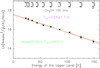 |
Fig. 6 Rotational diagram of the 13–17 Dec average of the methanol lines around 166 GHz in comet 46P/Wirtanen. The neperian logarithm of a quantity proportional to the line intensity is plotted against the energy of the upper level of each transition. Fit is shown by solid red line and errors are displayed by red dashed lines. The black dots are the measurements and green circles the predicted values for a model with a gas temperature of 60 K. |
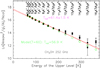 |
Fig. 7 Same as for Fig. 6, but for the 252 GHz lines of methanol observed between 11.8 and 17.8 Dec UT. |
Rotational temperatures and inferred gas kinetic temperatures.
5 Production rates and abundances
We determine the production rate or an upper limit for 35 molecules. We assumed that all species follow a parent or daughter Haser density distribution with a destruction scale length, as discussed in the next section and listed in Table 4. CS and SO are assumed to come from the photo-dissociation of CS2 and SO2, respectively.H2CO, as specified in Table 6, is assumed to come from a distributed source with a scale length of 5000 km (Biver et al. 1999), which fits observations obtained at various offsets and with different beam sizes (lines observed at 2 and 1 mm wavelengths). All production rates are provided in Tables 5 and 6.
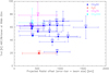 |
Fig. 9 All rotational temperatures as a function of the projected pointing offset and beam size (indicating which region of the coma is probed). Most values are compatible with a constant gas temperature of ≈60 K throughout the coma. This includes some low rotational temperature values such as that derived for H2 S lines, of which the rotational levels are not expected to be thermalised. |
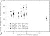 |
Fig. 10 Daily gas temperatures Tgas derived from the methanol rotational lines around 167, 213–230, 242, and 252 GHz as presented in the first part of Table 3. Variations cannot be related to the rotation of the nucleus (when folded on a single 9 h period). Most of the dispersion is due to the different series of methanol lines used: the 252 GHz ones sample a smaller region than the others and keep memory of Tgas at larger cometocentric distances than those at 242 GHz. |
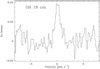 |
Fig. 11 Eighteen-centimetre OH line of comet 46P/Wirtanen observed with the Nançay radio telescope from 12 to 20 December 2018. The 1665 and 1667 MHz lines, both circular polarisations scaled to the 1667 MHz line, have been averaged. |
5.1 Molecular lifetimes
One major source of uncertainty for the abundance of several (complex) molecules is their photo-destruction rate (dissociation and ionisation). For a molecule with a short lifetime, the uncertainty in the retrieved production rate can be as large as the uncertainty in the photo-destruction rate, but thanks to the proximity of comet 46P/Wirtanen to the Earth (0.08 au), the small beam size of IRAM mostly probed ‘young’ molecules: 90% of the signal comes from molecules younger than ≈ 2.5 × 10³ s, which should reduce the impact of the uncertainty in their photolytic lifetime. In addition, the solar activity was close to a deep minimum, which caused the photo-dissociation rates to be close to their minimum values and reduced other effects such as, for example, dissociative impact from ions.
Table 4 summarises the latest information available on the lifetime of these molecules and the values that we adopted. For some well-observed molecules, we applied a solar-activity-dependent correction based on the 10.7-cm solar flux unit (70sfu on average for the period, mostly representative of the “quiet” Sun) as in Crovisier (1989). For several molecules, there is a large range of published values for their photo-destruction rate, or no values at all. For detected molecules, we can also obtain some constraints from their line shape. Since the expansion velocity generally increases with distance from the nucleus (e.g. acceleration due to photolytic heating), molecules with longer lifetimes will likely exhibit broader lines. This was clearly evidenced for comets at small heliocentric distances (Biver et al. 2011). Table 4 and details hereafter provide some loose constraints we can derive for some molecules. Observational data used for this purpose are presented in Appendix D. The H2 S, HCN, and CH3OH molecules have well established photo-dissociation rates, which can be used as references. We note that radiative excitation can also affect the line width, for example if the upper rotational state of the observed transition is depopulated at a faster rate than it is modelled. However, in that case a bias in the lifetime compensates for the weakness of the excitation model. For secondary species such as CS, SO, and H2CO, on the otherhand, any excess energy converted into velocity might affect the line shape, especially outside the collision-dominated region.
HC3N
In Biver et al. (2011), cyanoacetylene clearly showed a narrower line than HCN, CH3OH, and CS because of its shorter lifetime. It was detected with a high resolution and high S/N in the comet Hale-Bopp in April–May 1997 (Bockelée-Morvan et al. 2000), but its line shape did not suggest a much shorter lifetime than HCN or CH3OH, while the mean width of HC3N line is closer to that of H2S in comet C/2014 Q2 (Biver et al. 2015, and Table D.1). Thus, the adopted photo-dissociation rate is in agreement with the range suggested by those observations.
CH3CN
Methyl cyanide has a relatively long lifetime according to Crovisier (1994) and Heays et al. (2017), but most observations, including those of 46P(Figs. 3 and 2, Table D.1), show lines with widths similar to or slightly smaller thanthose of HCN or methanol. This suggests that its photo-destruction rate might be a few times larger than assumed, although this does not affect the retrieved production rate in comet 46P. In addition the rotational and derived kinetic temperature of CH3CN is most often comparable to or higher than the one derived from CH3OH (Fig. 9), again suggesting that the CH3CN lines might probe the inner coma more, which is compatible with a shorter lifetime. Assuming β0 = 2 × 10⁻⁵ s−1 for the observations of comet 46P will not increase the production rate by more than 2%, which is negligible.
Sum of photo-dissociation and photo-ionisation rates of the molecules at rh = 1.0 au.
Daily production rates in comet 46P in December 2018.
NH2CHO
The lifetime of formamide is poorly known, but constraints from observations already discussed in Biver et al. (2014) and from line widths do suggest that its photo-destruction rate from Heays et al. (2017), similarly to the value we adopted, is a good estimate.
CO
The lifetime of carbon monoxide is very long, but the CO line never shows a width larger than the species with a photo-dissociation rate around β0 = 10−5 s−1. Rather than an underestimation of its photo-ionisation or dissociation rate, this might be the result of, for example, a low translational collisional cross-section, which would make CO less sensitive to gas acceleration by photolytic heating, given the small size and dipole moment of the molecule.
CH3CHO
Acetaldehyde has now been detected in six comets, and in all cases the width of the CH3CHO lines is smaller than those of HCN and CH3OH but slightly larger than that of H2S. Huebner & Mukherjee (2015) and Heays et al. (2017) suggested higher photo-destruction rates (β0 = 18 × 10−5 s−1) than the one we have used so far (Crovisier et al. 2004a), but it is compatible with the observations. This might increase the retrieved abundance in comets observed further away from the Earth, but for comet 46P it only increases it by ~ 8%. However, in the case of comet C/2013 R1 (Biver et al. 2014), if the lifetime of CH3CHO is shorter than assumed, this might also significantly increase its abundance as it gets closer to the Sun, and this would need to be explained.
Average production rates in 46P in December 2018.
HCOOH
There are few observations of formic acid with a good S/N (mostly in Hale-Bopp and C/2014 Q2), but they all suggest that HCOOH does not expand much faster than H2 S, so its photo-destruction rate might be closer to β0 = 10 × 10−5 s−1, but it is likely not as large as was suggested by Huebner & Mukherjee (2015). Using this value or the one of Crovisier (1994) does not affect the abundance determination in 46P, but if we use β0 = 90 × 10−5 s−1 instead, as suggested by Huebner & Mukherjee (2015), the limit on the abundance in 46P is 40% higher, and likely to be much higher in other comets.
(CH2OH)2
Ethylene glycol has an unknown lifetime, but since the first identification of this molecule in a comet (Crovisier et al. 2004a), we used β0 = 2 × 10⁻⁵ s−1. There are few high spectral resolution detections with a good S/N. Biver et al. (2014, 2015) and Biver & Bockelée-Morvan (2019) show the average of several lines in a few comets: the line shape is generally narrower than it is for HCN and CH3OH, but the uncertainty is too large for definite conclusions – except in C/2014 Q2, where it seems clearly narrower than for HCN lines. A lifetime a few times shorter than assumed is possible. As for HCOOH, an underestimate of the photo-destruction rate could explain the apparent decrease in abundance at lower heliocentric distances observed in comet C/2013 R1 (Biver et al. 2014). Using β0 = 5 × 10⁻⁵ s−1 for comet 46P will not change the retrieved production rate.
H2CS
Thioformaldehyde was first detected through a single line in the comet Hale-Bopp (Woodney et al. 1999). Since that time, it has only been observed with sufficient spectral resolution and S/N in the comet C/2014 Q2 (Biver et al. 2015), although this is insufficient to accurately measure the line width. The line width seems barely larger than the H2 S one. Therefore, in the absence of any photolysis information, a lifetime comparable to or a bit longer than H2 S looks like a reasonable assumption.
CH3NH2
Methylamine has not yet been detected remotely in comets. We assumed β0 = 2 × 10⁻⁴ s−1 in Biver & Bockelée-Morvan (2019), which is comparable to the value from Heays et al. (2017) but lower than the one referred to in Crovisier (1994).
CH3SH
Methanethiol (or methyl mercaptan) has only been detected in situ in comet 67P with an abundance relative to water of 0.04% (Rubin et al. 2019). In Crovisier et al. (2004a), we assumed a photo-dissociation rate β0 = 10−4 s−1, whereas recent evaluations give values 25× or 3× higher (Huebner & Mukherjee 2015; Heays et al. 2017), with some confidence. With such short lifetimes, the assumed value of β0 (CH3SH) will directly impact the retrieved abundance. We will use β0 = 5 × 10⁻⁴ s−1. With the Huebner & Mukherjee (2015) value, which is 5× higher, the retrieved production rate (upper limit) would be a factor of 2 higher.
For other molecules, either the available photo-destruction rates are compatible with observations, or no information at all is available and we must rely on a priori values β0 =2–10 × 10−4 s−1 as used in some previous studies (e.g. Crovisier et al. 2004a,b) generally based on similar molecules. Figure E.1 can be used to infer the change of column density and inversely the production rate, due to a change in the photo-destruction rate.
5.2 Evolution of production rates
As we observed several molecules regularly (such as HCN, which was mapped daily to check the pointing, or CH3OH, which showslines in every observing setup), we also looked for daily variations of the activity. Table 5 provides the derived production rates for each time interval, corresponding to 1–2 h integration on a specific observing setup. The values are derived from both the on-nucleus pointing and offset positions when the S/Ns are high enough (e.g. HCN). Production rates are given for the four molecules (HCN, CH3OH, CH3CN, and H2 S) that are detected with sufficient S/Ns at different epochs. Production rates as a function of time are shown in Fig. 12. Time variations do not exceed ± 20–30% from the average value. An apparent rotation period of ≈9 h was reported (Handzlik et al. 2019; Moulane et al. 2019; Farnham et al. 2021), and we tried to fold the production rates or line Dopplershift values on periods of 4 to 18 h, but no clear pattern appears for a specific period.
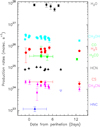 |
Fig. 12 Evolution of production rates in comet 46P/Wirtanen between 12 and 25 December 2019 (perihelionwas on 12.9 Dec.) for the nine main molecules. Downward-pointing empty triangles are 3-σ upper limits. Coloured symbols are in the vertical order of the corresponding molecules’ names on the right. Water production rates have been computed from data in Lis et al. (2019). |
5.3 Upper limits
Table 6 lists a large number of upper limits on the production rate of various molecules of interest. Besides the detection of some complex organic molecules (Biver & Bockelée-Morvan 2019), these observations were also the most sensitive ones ever undertaken in a Jupiter-family comet. In most cases, we only took into account collisions and radiative decay to compute theexcitation. We did not take into account infrared pumping via the rotational bands. The comet was not very active, so the collision region was not large, but due to its proximity to the Earth (0.08 au), the IRAM beam was still probing regions (within 1000 km) unlikely to be affected by infrared pumping. As discussed in Sect. 5.1, we probed molecules younger than about 2500 s so that any radiative (IR-pumping, photo-destruction) process that takes longer (g-factor, β0 < 4 × 10⁻⁴ s−1) would not significantly affect the expected signal and derived production rate. The corresponding upper limits in abundances relative to water are given in Table 7.
5.4 Relative abundances
Table 7 provides the mean abundances relative to water or upper limits derived from this study. Table 7 also lists values derived in other comets from ground-based observations (e.g. Biver & Bockelée-Morvan 2019) and from in situ observations in comet 67P. Abundances in comet 67P must be taken with caution when comparing to those measured in comet 46P/Wirtanen since the technique was often very different. In comet 67P, for some of the main species (e.g. CO, HCN, CH3OH, H2 S) Läuter et al. (2020) or Biver et al. (2019) derived relative bulk abundances from the integration of molecular loss over 2 yr. They also use different techniques: numerous local samplings by mass spectroscopy (with the Rosetta Orbiter Spectrometer for Ion and Neutral Analysis – ROSINA) vs. sub-millimetre mapping of the whole coma of some transitions (with the Microwave Instrument for the Rosetta Orbiter – MIRO), and they show some discrepancies. For species of lower abundances, mass spectroscopy with ROSINA is mostly based on specific observing campaigns at specific times (e.g. before perihelion, Rubin et al. 2019) and may not be representative of the bulk abundance of the species. Most complex organic molecules seem to be depleted in comet 67P, which could be due to this observational bias, or it could be more specific to 67P. Comet 46P has a composition quite comparable to most comets, although some species such as HC3N, HNCO, HNC, CS, and SO2 seem to be relatively under-abundant.
5.5 Isotopic ratios
The proximity to the Earth of comet 46P/Wirtanen offered a rare opportunity to attempt measurements of isotopic ratios in a Jupiter-family comet. However, limited information was obtained due to the relatively low activity level of the comet. The derived upper limit for the deuterium-to-hydrogen ratio (D/H) in water (Table 8) is five times higher than the D/H value of 1.61 ± 0.65 × 10⁻⁴ measured with SOFIA from the detection of the 509 GHz HDO line (Lis et al. 2019). Only H S could be clearly detected (Fig. 13). The 32 S/34S in H2S and the limits obtained in comet 46P for other isotopologues, with comparison to other references, are provided in Table 8. The 32 S/34S in H2S is compatible with the terrestrial value. HC15N shows a marginal 3 − σ signal both in the FTS and VESPA backends leading to 14 N/15N = 77 ± 26. This is significantly lower than the mean value (≈150, Biver et al. 2016)observed in cometary HCN, suggesting that this signal could be spurious.
6 Discussion and conclusion
6.1 Comparison with other observations
Comet 46P/Wirtanen was the target of a worldwide observing campaign in December 20182. It was observed with other millimetre-to-sub-millimetre facilities such as JCMT (Coulson et al. 2020), ALMA (Roth et al. 2020; Biver et al.,in prep.), and the Purple Mountain Observatory (Wang et al. 2020), which yield similar abundances. The short-term variation of the methanol line shifts and intensity, likely related to nucleus rotation, are observed in ALMA data (Roth et al. 2020, 2021).
Other observations (Moulane et al. 2019; Handzlik et al. 2019) suggest an excited rotation state of the nucleus with a primary period around 9 h at the time of the observations. The temporal sampling of our data set does notallow us to investigate time variations related to nucleus rotation. Infrared observations of comet 46P/Wirtanen (Dello Russo et al. 2019; Bonev et al. 2020; Khan et al. 2020) with the IRTF and Keck Telescope were obtained at similar times: they find similar methanol production rates, and that, compared to mean abundances measured among comets, 46P is relatively methanol rich, while it presents typical abundances of C2 H2, C2 H6, and NH3.
Molecular abundances.
Isotopic ratios.
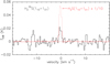 |
Fig. 13 H |


6.2 Comparison with other comets
Table 7 gives the abundances relative to water, or upper limits we derived in comet 46P/Wirtanen and a comparison with values measured in all other comets from millimetre-to-sub-millimetre ground-based observations and values measured in situ in comet 67P. Besides the differences in abundances relative to water between 46P and 67P due to different techniques (Sect. 5.4), the abundances found in comet 46P match most of those measured in other comets. However, some species seem rather depleted: CO (as is often observed in short period comets), HNCO, HCOOH, HNC, CS, and SO2. This is not surprising for HNC, which is produced by a distributed source and therefore rarefied within small fields of view (Cordiner et al. 2014). Assuming that it comes from a distributed source with a parent scale length of 1000 km (Cordiner et al. 2014, 2017), we find a HNC/HCN of 3.3%, 2.7× higher, but still relatively low in comparison to other comets observed at rh = 1 au. HNC was not detected in comet 73P-B (Lis et al. 2008), which was observed at a similarly small geocentric distance: the same interpretation could apply. Although we assumed that CS is produced from the photo-dissociation of CS2 , its abundance is still lower than in other comets, as suggested in Coulson et al. (2020). The presence of another distributed source of CS, which was proposed to explain the variation of its abundance with heliocentric distance (Biver et al. 2011) could explain this low abundance. Likewise, a possible interpretation for the HCOOH depletion in the inner coma of 46P is its production in the coma from the degradation of the ammonium salt NH HCOO−, which was observed in 67P (Altwegg et al. 2020).
6.3 Conclusion
We undertook a sensitive survey at millimetre wavelengths of the Jupiter-family comet 46P/Wirtanen in December 2018 at its most favourable apparition. This allowed us to detect 11 molecules and obtain sensitive upper limits on 24 other molecules. This is the most sensitive millimetre survey of a Jupiter-family comet regarding the number of measured molecular abundances.
Because the observations probed the inner coma (< 1000 km), the inferred abundances are weakly affected by uncertainties in molecular radiative and photolysis lifetimes. The abundances of complex molecules in 46P (e.g. CH3CHO, (CH2OH)2, NH2CHO, C2 H5OH) are similar to values measured in long period comets. However, CH3OH is more abundant. C2 H5OH/CH3OH is lower (3%) than in C/2014 Q2 (5.3%), C/2013 R1 (~ 6.5%), or Hale-Bopp (~8%).
Some molecules are particularly under-abundant in comet 46P, with CO <1.2%, which is often the case in JFCs, HNC, HNCO, and HCOOH. A likely explanation for the depletion of these acids in the inner coma of 46P is a production by distributed sources. There are several lines of evidence, including maps, that HNC is produced by the degradation of grains in cometary atmospheres (Cordiner et al. 2014, 2017). Ammonium salts, including NH +HCOO−, NH
 +OCN−, and NH
 +CN− have been identified in 67P’s dust grains, impacting the ROSINA sensor (Altwegg et al. 2020). Our measurements in 46P are consistent with HCOOH, HNCO, and HNC being produced by the sublimation of ammonium salts. The low CS abundance in 46P (0.03% vs. 0.05–0.20% measured in other comets 1 au from the Sun) suggests a distributed source of CS, other than CS2 , in cometaryatmospheres. The investigation of isotopic ratios only yielded the measurements of the 32 S/34S in H2S, which is consistent with the terrestrial value.
Acknowledgements
This work is based on observations carried out under projects number 112-18 with the IRAM 30-m telescope and project number W18AB with the NOEMA Interferometer. IRAM is supported by the Institut Nationnal des Sciences de l’Univers (INSU) of the French Centre national de la recherche scientifique (CNRS), the Max-Planck-Gesellschaft (MPG, Germany) and the Spanish IGN (Instituto Geográfico Nacional). We gratefully acknowledge the support from the IRAM staff for its support during the observations. The data were reduced and analysed thanks to the use of the GILDAS, class software (http://www.iram.fr/IRAMFR/GILDAS). This research has been supported by the Programme national de planétologie de l’Institut des sciences de l’univers (INSU). The Nançay Radio Observatory is operated by the Paris Observatory, associated with the CNRS and with the University of Orléans. Part of this research was carried out at the Jet Propulsion Laboratory, California Institute of Technology, under a contract with the National Aeronautics and Space Administration. B.P. Bonev and N. Dello Russo acknowledge support of NSF grant AST-2009398 and NASA grant 80NSSC17K0705, respectively.N.X. Roth was supported by the NASA Postdoctoral Program at the NASA Goddard Space Flight Center, administered by Universities Space Research Association under contract with NASA. M.A. Cordiner was supported in part by the National Science Foundation (under Grant No. AST-1614471). S.N. Milam and M.A. Cordiner acknowledgethe Planetary Science Division Internal Scientist Funding Program through the Fundamental Laboratory Research (FLaRe) work package, as well as the NASA Astrobiology Institute through the Goddard Center for Astrobiology (proposal 13-13NAI7-0032). M. DiSanti acknowledges support through NASA Grant 18-SSO18_2-0040.
Appendix A Supplementary line list table
Line intensities from IRAM and NOEMA observations.
Appendix B Full IRAM 30-m spectra of comet 46P/Wirtanen at 2 mm
The following pages present the 147–185 GHz (λ = 2 mm) FTS spectrum of comet 46P/Wirtanen obtained between 13.0 and 17.1 Dec 2018 with the IRAM 30-m telescope. The three wavelength domains covered are plotted by series of ≈ 2 GHz windows with a spectral resolution smoothed to 0.78 MHz. Only spectra obtained within 2′′ of the nucleus were taken into account, and the strongest lines are identified. We note the much higher noise level around the frequency of the atmospheric H2O line at 18 3310 MHz.
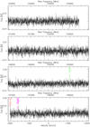 |
Fig. B.1 Vertical scale in main beam brightness temperature adjusted to the lines or noise level. The frequency scale in the rest frame of the comet is indicated on the upper axis. A velocity scale with a reference at the centre of each band is indicated onthe lower axis. |
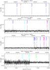 |
Fig. B.1 continued. |
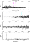 |
Fig. B.1 continued. |
Appendix C Full IRAM 30-m spectra of comet 46P/Wirtanen at 1 mm
The following pages present the 210–272 GHz (λ = 1.3 mm) FTS spectrum of comet 46P/Wirtanen obtained between 11.9 and 18.1 Dec 2018 with the IRAM 30-m telescope. The 62 GHz, ~ 320 000 channel spectrum is plotted in 6 × 4 series of ≈2.6 GHz windows with a spectral resolution smoothed to 0.78 MHz. These spectra were obtained with four receiver tunings each covering 2 × 7.78 GHz. There are some overlaps and gaps in the final 62 GHz-wide frequency coverage. Only spectra obtained within 3′′ from the nucleus were taken into account. The strongest lines (signal >2.5 × ⟨σ⟩) are labelled. Some identifications might be misleading where the local noise is higher than ⟨ σ⟩ and a noise peaks falls on a known molecular line resulting in a spurious detection.
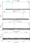 |
Fig. C.1 Vertical scale in main beam brightness temperature adjusted to the lines or noise level. The frequency scale in the rest frame of the comet is indicated on the upper axis. A velocity scale with reference at centre of each band is indicated onthe lower axis. The feature close to 230.5 GHz is due to contamination by galactic CO. |
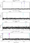 |
Fig. C.1 continued. |
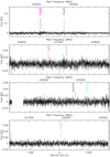 |
Fig. C.1 continued. |
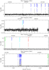 |
Fig. C.1 continued. |
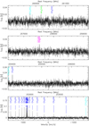 |
Fig. C.1 continued. |
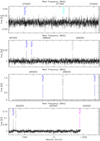 |
Fig. C.1 continued. |
Appendix D Selected molecular line widths in comets
Table D.1 provides the full width at half maximum (FWHM) or velocity at half maximum (VHM) for asymmetric double peak lines, from Gaussian fitting for molecular lines in comets. We took the average of several lines when possible, and observations with similar beam sizes for a given comet, in order to avoid being biased by spatial sampling. When a (small) trend of line widths with beam size is observed, the width has been interpolated to the mean beam size of the dataset. The objective is to correlate the line width with the molecule lifetime (when it is well known) or to constrain the lifetime of the molecule from its line width (when it is poorly known), as described in Sect. 5.1.
Molecular line width in comets in m s−1.
Appendix E Dependence of the production rate on the uncertainty in photo-destruction rate
Figure E.1 is provided here for the mean observing circumstances of the observations of comet 46P with IRAM 30-m telescope. In a first approximation, the line intensity is proportional to the column density Nc , which is itself proportional to the molecular production rate Q. So, for a given observed line intensity, a change of Nc due to a change of the photo-destruction rate β0, has to be compensated by an inverse change of Q:  .
.
From this plot, we can directly determine the change of the derived production rate Q when we change the value β0. For example, if β0 is increased from 2 to 20 × 10−5 s−1, we get  , meaning the retrieved production rate will be increased by only 12%. More generally, if the photo-destruction rate is not known but can be assumed to be less than that of H2S, an error of less than 16% on the retrieved production rate is anticipated from these observations of comet 46P.
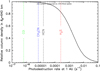 |
Fig. E.1 Evolution of the number of molecules in the IRAM 30-m beam as a function of molecule photo-destruction rate. We plot, more precisely, the average column density (number of molecules divided by the beam area) normalised to its value for infinite lifetime. We used the average beam size (θb = 11′′) for an average pointing offset of 2′′ at a geocentric distance of 0.08 au, which is typical for most observations of comet 46P. A change of molecular photo-destruction rate will result in a change of the column density that can be inferred from this plot. The position of the photo-destruction rate for well-known molecules is indicated. |
References
- A’Hearn, M. F., Millis, R. L., Schleicher, D. G., Osip, D. J., & Birch, P. V. 1995, Icarus, 118, 223 [Google Scholar]
- Altwegg, K., & Bockelée-Morvan, D. 2003, Space Sci. Rev., 106, 139 [Google Scholar]
- Altwegg, K., & the ROSINA Team 2018, Astrochemistry VII – Through the Cosmos from Galaxies to Planets. Proceedings IAU Symposium No. 332, eds. M. Cunningham, T. Millar, & Y. Aikawa [Google Scholar]
- Altwegg, K., Balsiger, H., Bar-Nun, A., et al. 2015, Science, 347, 1261952 [Google Scholar]
- Altwegg, K., Balsiger, H., Hänni, N., et al. 2020, Nat. Astron., 4, 533 [Google Scholar]
- Biver, N., & Bockelée-Morvan, D. 2019, ACS Earth Space Chem., 3, 1550 [Google Scholar]
- Biver, N., Bockelée-Morvan, D., Crovisier, J., et al. 1999, AJ, 118, 1850 [NASA ADS] [CrossRef] [Google Scholar]
- Biver, N., Bockelée-Morvan, D., Crovisier, J., et al. 2002, Earth Moon Planets, 90, 323 [Google Scholar]
- Biver, N., Bockelée-Morvan, D., Crovisier, J., et al. 2006, A&A, 449, 1255 [NASA ADS] [CrossRef] [EDP Sciences] [Google Scholar]
- Biver, N., Bockelée-Morvan, D., Crovisier, J., et al. 2007, Planet. Space Sci., 55, 1058 [Google Scholar]
- Biver, N., Bockelée-Morvan, D., Colom, P., et al. 2011, A&A, 528, A142 [NASA ADS] [CrossRef] [EDP Sciences] [Google Scholar]
- Biver, N., Bockelée-Morvan, D., Debout, V., et al. 2014, A&A, 566, L5 [Google Scholar]
- Biver, N., Bockelée-Morvan, D., Moreno, R., et al. 2015, Sci. Adv., 1, e1500863 [Google Scholar]
- Biver, N., Moreno, R., Bockelée-Morvan, D., et al. 2016, A&A, 589, A78 [NASA ADS] [CrossRef] [EDP Sciences] [Google Scholar]
- Biver, N., Bockelée-Morvan, D., Paubert, G., et al. 2018, A&A, 619, A127 [NASA ADS] [CrossRef] [EDP Sciences] [Google Scholar]
- Biver, N., Bockelée-Morvan, D., Hofstadter, M., et al. 2019, A&A, 630, A19 [NASA ADS] [CrossRef] [EDP Sciences] [Google Scholar]
- Bockelée-Morvan, D., Lis, D. C., Wink, J. E., et al. 2000, A&A, 353, 1101 [Google Scholar]
- Bockelée-Morvan, D., Hartogh, P., Crovisier, J., et al. 2010, A&A, 518, L149 [NASA ADS] [CrossRef] [EDP Sciences] [Google Scholar]
- Bockelée-Morvan, D., Calmonte, U., Charnley, S., et al. 2015, Space Sci. Rev., 197, 47 [Google Scholar]
- Boissier, J., Bockelée-Morvan, D., Biver, N., et al. 2007, A&A, 475, 1131 [NASA ADS] [CrossRef] [EDP Sciences] [Google Scholar]
- Bonev B. P., Dello Russo, N., DiSanti, M. A. et al. 2020, Planet. Sci. J., 2, 45 [Google Scholar]
- Brasser, R., & Morbidelli, A. 2013, Icarus, 225, 40 [NASA ADS] [CrossRef] [Google Scholar]
- Carter, M, Lazareff, B., Maier, D., et al. 2012, A&A, 538, A89 [NASA ADS] [CrossRef] [EDP Sciences] [Google Scholar]
- Combi, M. R., Mäkinen, T., Bertaux, J. L., et al. 2020, Planet. Sci. J., 1, 72 [Google Scholar]
- Cordiner, M. A., Remijan, A. J., Boissier, J., et al. 2014, ApJ, 792, 2 [Google Scholar]
- Cordiner, M. A., Boissier, J., Charnley, S. B., et al. 2017, ApJ, 838, 147 [Google Scholar]
- Cordiner, M. A., Palmer, M. Y., de Val-Borro, M., et al. 2019, ApJ, 870, L26 [Google Scholar]
- Coulson, I. M., Liu, F.-C., Cordiner, M. A., et al. 2020, AJ 160, 182 [Google Scholar]
- Crovisier, J. 1989, A&A, 213, 459 [NASA ADS] [Google Scholar]
- Crovisier, J. 1994, J. Geophys. Res., 99 E2, 3777 [Google Scholar]
- Crovisier, J., Colom, P., Gérard, E., Bockelée-Morvan, D., & Bourgois, G. 2002, A&A, 393, 1053 [NASA ADS] [CrossRef] [EDP Sciences] [Google Scholar]
- Crovisier, J., Bockelée-Morvan, D., Colom, P., et al. 2004a, A&A, 418, 1141 [NASA ADS] [CrossRef] [EDP Sciences] [Google Scholar]
- Crovisier, J., Bockelée-Morvan, D., Biver, N., et al. 2004b, A&A, 418, L35 [NASA ADS] [CrossRef] [EDP Sciences] [Google Scholar]
- Dello Russo, N., McKay, A. J., Saki, M., et al. 2019, EPSC-DPS2019 abstract #742 [Google Scholar]
- Despois, D., Gerard, E., Crovisier, J., & Kazes, I. 1981, A&A, 99, 320 [Google Scholar]
- Farnham, T. L., Knight, M. M., Schleicher, D. G., et al. 2021, Planet. Sci. J., 2, 7 [Google Scholar]
- Greenstein, J. L. 1958, ApJ, 128, 106 [Google Scholar]
- Hadraoui, K., Cottin, H., Ivanovski, S. L., et al. 2019, A&A, 630, A32 [CrossRef] [EDP Sciences] [Google Scholar]
- Handzlik, B., Drahus, M., & Kurowski, S. 2019, EPSC-DPS2019 abstract #1775 [Google Scholar]
- Hartogh, P., Lis, D. C., Bockelée-Morvan, D., et al. 2011, Nature, 478, 218 [Google Scholar]
- Heays, A. N., Bosman, A. D., & van Dishoeck, E. F. 2017, A&A, 602, A105 [NASA ADS] [CrossRef] [EDP Sciences] [Google Scholar]
- Huebner, W. F., & Mukherjee, J. 2015, Planet. Space Sci., 106, 11 [Google Scholar]
- Huebner, W. F., Keady, J. J., & Lyon, S. P. 1992, Ap&SS, 195, 1 [NASA ADS] [CrossRef] [Google Scholar]
- Irvine, W. M., Senay, M., Lovell, A. J., et al. 2000, Icarus, 143, 412 [Google Scholar]
- Khan, Y., Gibb, E. L., Bonev, B. P., et al. 2020, Planet. Sci. J., 1, 20 [Google Scholar]
- Läuter, M., Kramer, T, Rubin, M., & Altwegg, K. 2020, MNRAS, 498, 3995 [Google Scholar]
- Lis, D. C., Bockelée-Morvan, D., Boissier, J., et al. 2008, ApJ, 675, L931 [Google Scholar]
- Lis, D. C., Bockelée-Morvan, D., Güsten, R., et al. 2019, A&A, 625, L5 [NASA ADS] [CrossRef] [EDP Sciences] [Google Scholar]
- Moulane, Y., Jehin, E., José Pozuelos, F., et al. EPSC-DPS2019 abstract #1036 [Google Scholar]
- Müller, H. S. P., Schlöder, F., Stutzki J., & Winnewisser, G. 2005, J. Mol. Struct., 742, 215 [Google Scholar]
- O’Brien, D. P., Walsh, K. J., Morbidelli, A., Raymond, S. N., & Mandell, A. M. 2014, Icarus, 239, 74 [Google Scholar]
- Pickett, H. M., Poynter, R. L., Cohen, E. A., et al. 1998, J. Quant. Spec. Radiat. Transf., 60, 883 [Google Scholar]
- Roth, N. X., Milam S. N., Cordiner M. A., et al. 2020, BAAS, 52-6, DPS abstract #108.03 [Google Scholar]
- Roth, N. X., Milam S. N., Cordiner M. A., et al. 2021, Planet. Sci. J., 2, 55 [Google Scholar]
- Rubin, M., Altwegg, K., Balsiger, H., et al. 2019, MNRAS, 489, 594 [CrossRef] [Google Scholar]
- Schleicher, D. G., & A’Hearn, M. F., 1988, ApJ, 331, 1058 [Google Scholar]
- Wang, Z., Zhang, S.-B., Tseng, W.-L., et al. 2020, AJ, 159, 240 [Google Scholar]
- Woodney, L. M., A’Hearn, M. F., McMullin, J., & Samarasinha, N. 1999, Earth Moon Planets, 78 , 69 [Google Scholar]
All Tables
Sum of photo-dissociation and photo-ionisation rates of the molecules at rh = 1.0 au.
All Figures
|
Fig. 1 Map of HCN(3-2) line-integrated intensity in comet 46P/Wirtanen on 17.82 Dec. 2018. Offsets are relative to JPL#181/16 position and corrected for estimated pointing errors. The direction of the Sun is indicated by the arrow in the upper right. Contours are drawn every 0.225 Kkm s−1. |
| In the text | |
|
Fig. 2 Molecular lines observed in comet 46P/Wirtanen between 11.9 and 18.1 Dec. 2018. For some complex organics, we averaged several lines between 210 and 272 GHz (1 mm wavelength band). The vertical scale is the main beam brightness temperatureand the horizontal scale is the Doppler velocity in the comet rest frame. |
| In the text | |
|
Fig. 3 Molecular lines observed in comet 46P/Wirtanen between 11.9 and 18.1 Dec 2018 in the 2 mm band, except for HC3 N and OCS, for which we show the weighted average of five lines expected in the 1 mm band. For some complex organics, we averaged several lines between 147 and 170 GHz (2 mm wavelength). The vertical scale is the main beam brightness temperatureand the horizontal scale is the Doppler velocity in the comet rest frame. |
| In the text | |
|
Fig. 4 Series of methanol lines around 242 GHz observed in comet 46P/Wirtanen between 12.0 and 17.9 Dec. 2018. The vertical scale is the main beam brightness temperature, and the horizontal scale is the Doppler velocity in the comet rest frame and frequency in the comet frame on the upper scale. |
| In the text | |
|
Fig. 5 Series of methanol lines around 252 GHz observed in comet 46P/Wirtanen between 11.8 and 17.8 Dec. 2018. The vertical scale is the main beam brightness temperature, and the horizontal scale is the Doppler velocity in the comet rest frame and frequency in the comet frame on the upper scale. |
| In the text | |
|
Fig. 6 Rotational diagram of the 13–17 Dec average of the methanol lines around 166 GHz in comet 46P/Wirtanen. The neperian logarithm of a quantity proportional to the line intensity is plotted against the energy of the upper level of each transition. Fit is shown by solid red line and errors are displayed by red dashed lines. The black dots are the measurements and green circles the predicted values for a model with a gas temperature of 60 K. |
| In the text | |
|
Fig. 7 Same as for Fig. 6, but for the 252 GHz lines of methanol observed between 11.8 and 17.8 Dec UT. |
| In the text | |
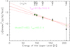 |
Fig. 8 Same as for Fig. 6, but for the 257 GHz lines of CH3CN observed between 12.0 and 17.9 Dec UT. |
| In the text | |
|
Fig. 9 All rotational temperatures as a function of the projected pointing offset and beam size (indicating which region of the coma is probed). Most values are compatible with a constant gas temperature of ≈60 K throughout the coma. This includes some low rotational temperature values such as that derived for H2 S lines, of which the rotational levels are not expected to be thermalised. |
| In the text | |
|
Fig. 10 Daily gas temperatures Tgas derived from the methanol rotational lines around 167, 213–230, 242, and 252 GHz as presented in the first part of Table 3. Variations cannot be related to the rotation of the nucleus (when folded on a single 9 h period). Most of the dispersion is due to the different series of methanol lines used: the 252 GHz ones sample a smaller region than the others and keep memory of Tgas at larger cometocentric distances than those at 242 GHz. |
| In the text | |
|
Fig. 11 Eighteen-centimetre OH line of comet 46P/Wirtanen observed with the Nançay radio telescope from 12 to 20 December 2018. The 1665 and 1667 MHz lines, both circular polarisations scaled to the 1667 MHz line, have been averaged. |
| In the text | |
|
Fig. 12 Evolution of production rates in comet 46P/Wirtanen between 12 and 25 December 2019 (perihelionwas on 12.9 Dec.) for the nine main molecules. Downward-pointing empty triangles are 3-σ upper limits. Coloured symbols are in the vertical order of the corresponding molecules’ names on the right. Water production rates have been computed from data in Lis et al. (2019). |
| In the text | |
|
Fig. 13 H |
| In the text | |
|
Fig. B.1 Vertical scale in main beam brightness temperature adjusted to the lines or noise level. The frequency scale in the rest frame of the comet is indicated on the upper axis. A velocity scale with a reference at the centre of each band is indicated onthe lower axis. |
| In the text | |
|
Fig. B.1 continued. |
| In the text | |
|
Fig. B.1 continued. |
| In the text | |
|
Fig. C.1 Vertical scale in main beam brightness temperature adjusted to the lines or noise level. The frequency scale in the rest frame of the comet is indicated on the upper axis. A velocity scale with reference at centre of each band is indicated onthe lower axis. The feature close to 230.5 GHz is due to contamination by galactic CO. |
| In the text | |
|
Fig. C.1 continued. |
| In the text | |
|
Fig. C.1 continued. |
| In the text | |
|
Fig. C.1 continued. |
| In the text | |
|
Fig. C.1 continued. |
| In the text | |
|
Fig. C.1 continued. |
| In the text | |
|
Fig. E.1 Evolution of the number of molecules in the IRAM 30-m beam as a function of molecule photo-destruction rate. We plot, more precisely, the average column density (number of molecules divided by the beam area) normalised to its value for infinite lifetime. We used the average beam size (θb = 11′′) for an average pointing offset of 2′′ at a geocentric distance of 0.08 au, which is typical for most observations of comet 46P. A change of molecular photo-destruction rate will result in a change of the column density that can be inferred from this plot. The position of the photo-destruction rate for well-known molecules is indicated. |
| In the text | |
Current usage metrics show cumulative count of Article Views (full-text article views including HTML views, PDF and ePub downloads, according to the available data) and Abstracts Views on Vision4Press platform.
Data correspond to usage on the plateform after 2015. The current usage metrics is available 48-96 hours after online publication and is updated daily on week days.
Initial download of the metrics may take a while.