| Issue |
A&A
Volume 690, October 2024
|
|
|---|---|---|
| Article Number | A271 | |
| Number of page(s) | 29 | |
| Section | Planets and planetary systems | |
| DOI | https://doi.org/10.1051/0004-6361/202450921 | |
| Published online | 11 October 2024 | |
Chemical composition of comets C/2021 A1 (Leonard) and C/2022 E3 (ZTF) from radio spectroscopy and the abundance of HCOOH and HNCO in comets★,★★
1
LESIA, Observatoire de Paris, PSL Research University, CNRS, Sorbonne Université, Université Paris-Cité,
5 place Jules Janssen,
92195
Meudon,
France
2
Astronomical Observatory, Jagiellonian University,
ul. Orla 171,
30-244,
Kraków,
Poland
3
Stockholm Observatory, Stockholm University, SCFAB-AlbaNova,
10691
Stockholm,
Sweden
4
IRAM,
300 rue de la Piscine,
38406
Saint Martin d’Hères,
France
5
Physikalish-Meteorologisches Observatorium Davos und Weltstrahlungszentrum (PMOD/WRC)
Dorfstrasse 33,
7260
Davos Dorf,
Switzerland
6
Jet Propulsion Laboratory, California Institute of Technology,
4800 Oak Grove Drive,
Pasadena,
CA
91109,
USA
7
Solar System Exploration Division,
Astrochemistry Laboratory Code 691, NASA-GSFC,
Greenbelt,
MD
20771,
USA
8
Department of Physics, Catholic University of America,
Washington,
DC
20064,
USA
9
Department of Physics, American University,
Washington,
DC,
USA
10
Johns Hopkins University Applied Physics Laboratory,
11100 Johns Hopkins Rd.,
Laurel,
MD
20723,
USA
11
Institute for Astronomy, University of Edinburgh, Royal Observatory,
Edinburgh
EH9 3HJ,
UK
12
Koyama Astronomical Observatory, Kyoto Sangyo University, Motoyama, Kamitamo, Kita,
Kyoto
603-8555,
Japan
★★★ Corresponding author; nicolas.biver@obspm.fr
Received:
30
May
2024
Accepted:
26
July
2024
We present the results of a molecular survey of long period comets C/2021 A1 (Leonard) and C/2022 E3 (ZTF). Comet C/2021 A1 was observed with the Institut de radioastronomie millimétrique (IRAM) 30-m radio telescope in November-December 2021 before perihelion (heliocentric distance 1.22 to 0.76 au) when it was closest to the Earth (≈0.24 au). We observed C/2022 E3 in January-February 2023 with the Odin 1-m space telescope and IRAM 30-m, shortly after its perihelion at 1.11 au from the Sun, and when it was closest to the Earth (≈0.30 au). Snapshots were obtained during 12–16 November 2021 period for comet C/2021 A1. Spectral surveys were undertaken over the 8–13 December 2021 period for comet C/2021 A1 (8 GHz bandwidth at 3 mm, 16 GHz at 2 mm, and 61 GHz in the 1 mm window) and over the 3–7 February 2023 period for comet C/2022 E3 (25 GHz at 2 mm and 61 GHz at 1 mm). We report detections of 14 molecular species (HCN, HNC, CH3CN, HNCO, NH2CHO, CH3OH, H2CO, HCOOH, CH3CHO, H2S, CS, OCS, C2H5OH and aGg’-(CH2OH)2) in both comets. In addition, HC3N, and CH2OHCHO were marginally detected in C/2021 A1, and CO and H2O (with Odin) were detected in C/2022 E3. The spatial distribution of several species (HCN, HNC, CS, H2CO, HNCO, HCOOH, NH2CHO, and CH3CHO) is investigated. Significant upper limits on the abundances of other molecules and isotopic ratios are also presented. The activity of comet C/2021 A1 did not vary significantly between 13 November and 13 December 2021, when observations stopped, just before it started to exhibit major outbursts seen in the visible and from observations of the OH radical. Short-term variability in the outgassing of comet C/2022 E3 of the order of ±20% is present and possibly linked to its 8h rotation period. Both comets exhibit rather low abundances relative to water for volatile species such as CO (<2%) and H2S (0.15%). Methanol is also rather depleted in comet C/2021 A1 (0.9%). Following their revised photo-destruction rates, HNCO and HCOOH abundances in comets observed at millimetre wavelengths have been reevaluated. Both molecules are relatively enriched in these two comets (~0.2% relative to water). Since the combined abundance of these two acids (0.1–1%) is close to that of ammonia in comets, we cannot exclude that these species could be produced by the dissociation of ammonium formate and ammonium cyanate if present in comets.
Key words: molecular data / comets: general / radio lines: planetary systems / submillimeter: planetary systems / comets: individual: C/2021 A1 (Leonard) / comets: individual: C/2022 E3 (ZTF)
Based on observations carried out with the IRAM-30m telescope. IRAM is supported by INSU/CNRS (France), MPG (Germany), and IGN (Spain).
Odin is a Swedish-led satellite project funded jointly by the Swedish National Space Board (SNSB), the Canadian Space Agency (CSA), the National Technology Agency of Finland (Tekes), the Centre National d’Études Spatiales (CNES, France), and the European Space Agency (ESA). The Swedish Space Corporation, today OHB Sweden, is the prime contractor, also responsible for Odin operations.
© The Authors 2024
 Open Access article, published by EDP Sciences, under the terms of the Creative Commons Attribution License (https://creativecommons.org/licenses/by/4.0), which permits unrestricted use, distribution, and reproduction in any medium, provided the original work is properly cited.
This article is published in open access under the Subscribe to Open model. Subscribe to A&A to support open access publication.
1 Introduction
Comets are the most pristine remnants of the formation of the Solar System 4.6 billion years ago. They sample some of the oldest and most primitive material in the Solar System, including ices, and are thus our best window on the volatile composition of the solar proto-planetary disk. Comets may also have played a role in the delivery of water and organic material to the early Earth (see Hartogh et al. 2011, and references therein). The latest simulations of the early Solar System’s evolution (Brasser & Morbidelli 2013; O’Brien et al. 2014) suggest a more complex scenario. On the one hand, ice-rich bodies that formed beyond Jupiter may have been implanted early in the outer asteroid belt and participated in the supply of water to the Earth. On the other hand, current comets are coming from either the Oort Cloud or the scattered disk of the Kuiper belt and may have formed in the same trans-Neptunian region, sampling the same diversity of formation conditions. Understanding the diversity in composition and isotopic ratios of cometary materials is thus essential for assessing such scenarios (Altwegg & Bockelée-Morvan 2003; Bockelée-Morvan et al. 2015).
Comet C/2021 A1 (Leonard) is a long-period dynamically old Oort-Cloud comet (OCC, with an initial semi-major axis of 2000 au and an inclination of 132.7°) that reached perihelion at a heliocentric distance rh=0.615 au on 3.3 January 2022 UT. It came as close as 0.234 au to the Earth on 12.6 December 2021. It was anticipated to become a bright comet visible to the naked eye, but it under-performed until 14 December when it was in solar conjunction. Then monitoring of the outgassing rate via observations of the OH radical (Crovisier et al. 2021) and visual magnitudes showed strong outbursts of activity, repeating on a ~5 day period from 15 December to 7 January 20221. Then, it developed spectacular ion and dust tails while being mostly observable from the southern hemisphere. Later on, the comet faded rapidly, and images taken in April–May 2022 suggest that it was disintegrating during this outbursting phase. The derived pre-disintegration nucleus radius was 0.6 ± 0.2 km (Jewitt et al. 2023). We observed comet C/2021 A1 with the Institut de radioastronomie millimétrique (IRAM) 30-m telescope briefly between 12.0 and 16.4 November, and extensively between 8.4 and 13.4 December 2021 UT, before it reached declinations that are too low for the northern observatories.
Comet C/2022 E3 (ZTF) is also a long-period dynamically old OCC (with an initial semi-major axis of 1400 au and an inclination of 109.2°). It reached perihelion at rh = 1.112 au on 12.8 January 2023 UT. It was closest to the Earth on 1.8 February 2023 at 0.284 au, and reached naked eye visibility (total magnitude of 4.8). It attracted public attention and was the target of a worldwide campaign because it was discovered 11 months ahead of its peak brightness, expected to happen at the end of January 2023 when the comet was circumpolar for the northern hemisphere and visible to the naked eye all night2. The comet was further advertised in NASA news releases at the end of 20213. We observed comet C/2022 E3 with the Odin space telescope from 19.3 to 20.3 January 2023 (Biver et al. 2023b) and with the IRAM-30m radio telescope between 3.7 and 7.1 February. Due to its high activity and a favourable apparition, this comet was the focus of an international observing campaign, from the radio – OH observed with the Nançay Radio Telescope (NRT) and the Green Bank Telescope – to the infrared (ground-based observations with IRTF and Keck-NIRSPEC and from space with the James Webb Space Telescope on 28 February and 4 March, Milam et al. 2023).
In this paper, we report clear detections of HCN, HNC, CH3CN, HNCO, NH2CHO, CH3OH, H2CO, HCOOH, H2S, and CS in both comets, the more marginal detections of CO, HC3N, CH3CHO, OCS, (CH2OH)2, CH2OHCHO, and C2H5OH, obtained by averaging several lines, as well as significant upper limits on the abundances of SO, SO2, H2CS, CH2CO, PH3, and other species.
In addition, following the revised photo-destruction rates of several molecules by Hrodmarsson & van Dishoeck (2023), especially of HNCO and HCOOH for which the lifetime has been reduced by nearly one order of magnitude in comparison to previously published or assumed destruction rates (Heays et al. 2017; Huebner & Mukherjee 2015; Biver et al. 2021a), we have reevaluated their abundances in all comets in which they were observed or searched for.
In Sect. 2, we present the observations and spectra of the detected molecules. The information extracted from the observations to analyse the data and compute production rates is provided in Sec. 3. In Sec. 4, we present the retrieved production rates and abundances or upper limits, which are discussed and compared to other comets. The new analysis of HNCO and HCOOH observations are detailed in Sec. 5 followed by the conclusions in Sec. 6.
2 Observations
2.1 Observations of comet C/2021 A1 with the IRAM-30m
Comet C/2021 A1 (Leonard)4 was the focus of a worldwide campaign as it was expected to become very bright at its closest approach to Earth (total visual magnitude m1 ~ 4). It was less active than anticipated until 14 December, when it started to undergo a series of recurrent outbursts bringing it to a maximum brightness of around m1 = 3 between 15 and 25 December 2021.
It was the target of the observing proposal 100-21 scheduled at the IRAM 30-m telescope between 8 and 13 December 2021. Weather conditions were marginal during the first four days (half of the day too icy, windy, or foggy to observe, with precipitable water vapour (pwv) in the 3 to 7 mm range otherwise). On the first day (observations were taking place during daytime), when observations resumed after an ice storm, the leftover ice or the impact of de-icing on the antenna reduced the beam efficiency by a factor of 3 (at 1 mm wavelength) to 1.5 (at 2 mm). The last two days offered good weather conditions with pwv = 1–3 mm (Table A.1). A few other snapshots (less than 0.5 h of observations) were obtained between 12 and 16 November during observing run 001-21 when comet 67P/Churyumov-Gerasimenko was too high in elevation for tracking (Biver et al. 2023a).
Observations were obtained in wobbler switching mode with the secondary (wobbling) mirror alternating pointing between the ON and OFF positions separated by 180″ every 2 seconds. The wobbler was not working on 14–16 November 2021 and we had to use to the position switching mode (PSW). The reference OFF positions in PSW mode were at 300″ from the source, alternating ON and OFF every 15 seconds. We used the EMIR (Eight MIxer Receiver, Carter et al. 2012) 3 mm, 2 mm, and 1 mm band receivers in 2SB mode connected to the FTS (Fast Fourier Transform Spectrometer) and the VESPA (VErsatile SPectrometer Array) high-resolution spectrometer (Table A.1). The FTS offers an instantaneous bandwidth of 16 GHz in two polarisations with 200 kHz spectral resolution. The VESPA autocorrelator was optimised to provide 4–6 windows of 20–40 kHz spectral resolution on lines of interest in the centre of the Intermediate Frequency windows (6.25 ± 0.25 GHz).
Comet C/2021 A1 was tracked with the IRAM-30m control software (NCS) using the latest JPL Horizons5 orbital elements available:#15 in November, #17 on 8 December, and #18 on 9–13 December 2021. Offsets (up to 7″) were added during the observation to take into account the difference between the position computed by the NCS and the very latest (1–3 days old) astrometric measurements. This was a critical point as for such a new comet relatively close to Earth, positions errors can easily reach the beam size (10″ at 240 GHz). The comet position was also checked in real time using coarse (5–9 points) mapping of HCN J=3–2 (Fig. 1). Ephemeris offsets were computed afterwards using the JPL#19 orbit solution (yielding values in agreement with the astrometry that was used). Final pointing offsets for each observation were computed after taking into account reconstruction of pointing errors and finally from intensity maps of HCN, that generally yielded residual offsets of less than 1.2″.
Representative spectra of comet C/2021 A1 (Leonard) are provided in Figs. 2 and 3 and Figs. A.1–A.3. They show individual lines or averages of several lines for the complex organics from the observations centred on the nucleus. Detailed line intensities are provided in Tables online and for some molecules with useful spatial information in Table B.5 of Sec. 4.3. Spectra showing the full spectral coverage with the wide band FTS are available online.
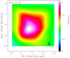 |
Fig. 1 Coarse map of the HCN(3–2) line integrated intensity in comet C/2021 A1 on 13.4 December 2021. The beam size is 9.3″. Solar phase angle was 158.6°. The direction of the Sun (PA=193.1°) is indicated at the lower right. |
2.2 Observations of comet C/2022 E3 (ZTF) with Odin
Comet C/2022 E3 (ZTF) was favourably placed (solar elongation between 60° and 120°) for Odin during one of its yearly astronomy science operations. 15 orbits (~24h) were dedicated to observe the H2O(110 − 101) line at 556.9 GHz in this comet. Odin (Frisk et al. 2003) is a small satellite in a polar orbit (period 95 min) equipped with a 1.1 m sub-millimetre radiometer. Odin houses four sub-mm receivers covering the 486–504 GHz and 541–581 GHz range with 3 backends: one acousto-optical-spectrometer (AOS) with 1 GHz band width and 1.2 MHz spectral resolution and two autocorrelators (AC1 and AC2), covering 120 MHz with 140 kHz resolution in their highest resolution mode. Two of the receivers, 555B2 and 549A1, were supposed to observe the 556.9 GHz line, but the 549A1 receiver did not lock, and we only obtained data from the 555B2 receiver connected to the AOS and AC2. We aimed at alternating between pointing on the comet position and coarse 3 × 3 points maps spaced by 60 or 120″. The beam size was 127″. Odin achieved successful tracking of the comet on most of 14 of the 15 orbits scheduled from 19.3 to 20.3 January 2023 UTC (Table A.2). Part of the data from the 13th and 14th orbits was lost also due to memory overload. Reconstruction of the attitude of Odin did not always converge with good accuracy due to the lack of reference stars in the star-trackers field of view, but most of the pointings were within 15″ (≈12% of the beam width) of the comet position. Figure 4 shows the result from the combination of all the maps.
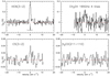 |
Fig. 2 Millimetre lines observed with IRAM-30m in comet C/2021 A1 during 12–16 November 2021 (average intensity). The CH3OH line is the sum of the J=1 to 4 J1 − J0 E lines at 165050.175, 165061.130, 165099.240, and 165190.475 MHz observed with the high resolution backend VESPA. The vertical axis is main beam brightness temperature in K and the horizontal axis is Doppler velocity in the rest frame of the comet with respect to the main line. |
2.3 Observations of comet C/2022 E3 (ZTF) with the IRAM-30m
Comet C/2022 E3 (ZTF) was the target of the observing proposal 097-22 scheduled at the IRAM 30-m telescope between 3 and 8 February 2023. Weather conditions were very good to good during the first four days (but too windy followed by a technical issue with the antenna temperature control during 2/3 of the first night). The last night (February 7/8) was lost due to bad weather (snow + wind). Pointing and focus stability was not very good at the beginning of the nights. Very low opacity on 5.0 February (0.2–1 mm pwv) enabled a short observation at 177–185 GHz, but the weather conditions degraded and the observing time was too limited to get a useful result on the H2O line at 183.3 GHz. Table A.2 provides a log of the observations.
Wobbler switching mode with the secondary (wobbling) mirror alternating pointing between the ON and OFF positions separated by 120″ every 2 seconds could only be used on the last night as it had again issues as in November 2021. We had to rely on position switching mode (PSW) with reference OFF positions at 240″, alternating ON and OFF every 15 seconds. Even using symmetric mode (ON OFF OFF ON sequence), alternating the reference position in +RA and -RA, leaves some residual at the position of the strong ozone atmospheric lines, where the spectra are noisier with poorer baselines, especially around 231.13, 237.17, 242.34, 249.80, 249.97, and 267.28 GHz, As for comet C/2021 A1, we used the EMIR receivers and the FTS and VESPA spectrometers (Sec. 2.1).
Comet C/2022 E3 was tracked with the IRAM-30m control software (NCS) using the latest JPL Horizons orbital elements available at the beginning of the observations, JPL#41, adding up offsets (~5″ in declination) from the latest astrometric measurements available and confirmed by coarse mapping of the strongest lines in the setup. Final offset in the reduced data take into account a more recent (JPL#45) orbit solution and reconstructed pointing corrections of the antenna to cope with potential approximations during real time observations (Fig. 5).
Representative spectra of comet C/2022 E3 (ZTF) are provided in Fig. 6 and Figs. A.4–A.6. They show individual lines or averages of several lines for the complex organics from the observations centred on the nucleus. Detailed line intensities are provided online, and for some molecules with useful spatial information in Table B.6 of Section 4.3. Spectra showing the full spectral coverage with the FTS are provided online.
Figs. A.3 and A.6 show the average of 3 to 97 lines, weighted according to the noise in each spectrum. We have selected the strongest lines with expected similar S/N (within a factor around four) which are not blended with other lines. This is only for the purpose of highlighting detection and line shapes.
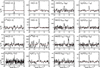 |
Fig. 3 Individual lines observed with IRAM-30m in comet C/2021 A1 during 8–13 December 2021 (weighted averages). The vertical axis is main beam brightness temperature in K and the horizontal axis is Doppler velocity in the rest frame of the comet with respect to the line. The position and relative intensity of the hyperfine components of the HCN(3–2) line have been drawn below the line. |
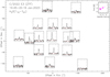 |
Fig. 4 Map of the average spectra of the H2O(110−101) line obtained with Odin between 19.45 and 20.16 January 2023 in comet C/2022 E3 (ZTF), as a function of the pointing offset (in arcsec). A baseline in red is plotted on each spectrum. Solar phase angle was 61.6°, and the direction of the Sun (PA=120.2°) is indicated at the upper right with scales for individual AC2 spectra. |
2.4 Observations with the Nançay Radio Telescope
The NRT performances and the observing procedure used for comets were described in Crovisier et al. (2002). The integration time is usually about one hour per day. However, from 12 September to 14 December 2021, it was limited to 30 min due to work on the focal track. The beam size at 18-cm wavelength is 3.5 × 18′.
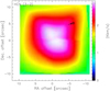 |
Fig. 5 Coarse (3×3 points) map of the HCN(3–2) line integrated intensity on 4.67 February 2023 in comet C/2022 E3. Solar phase angle was 45.5°. The direction of the Sun (PA=287°) is indicated at the upper right. |
2.4.1 Comet C/2021 A1 (Leonard)
C/2021 A1 (Leonard) was observed at the NRT from 1 October 2021 to 14 February 2022 almost every day or every other day6.
A succession of outbursts was observed, beginning on 13 December just at the end of the IRAM observations (Crovisier et al. 2021; Jehin et al. 2021). The OH production rate, which was 2.5 ± 0.1 × 1028 molecules s−1 on average for 8–12 December, rose to 6.3 ± 0.3 × 1028 molecules s−1 on 13.5, up to 22.1 ± 0.2 × 1028 molecules s−1 on 15.5 December.
Representative spectra for selected dates are shown in Fig. 7. The evolution of the retrieved OH production rate is plotted in Fig. 8.
2.4.2 Comet C/2022 E3 (ZTF)
C/2022 E3 (ZTF) was observed at the NRT from 17 October to 23 December 20227 The retrieved OH production rate rose from 3.3 to 8.1 × 1028 molecules s−1. Then the observations were interrupted due to a technical failure on 24 December 2022. They were resumed from 17 to 24 February 2023 in a degraded mode, resulting in an upper limit Q(OH) ≤ 6 × 1028 molecules s−1.
3 Data analysis
3.1 Expansion velocity and outgassing pattern
The lines profiles (Figs. 2–3) of comet C/2021 A1 do not show systematic asymmetry, excepted for small shifts with respect to the rest velocity in the comet frame. In November the mean Doppler shift of the line is slightly negative (δv = −0.03 ± 0.03 km s−1 for HCN(3–2)) and positive for most lines in December (δv(HCN(3–2))= +0.18 ± 0.01 km s−1). The two-Gaussian fit (Biver et al. 2021a) used to estimate the expansion velocity from the velocity at half maximum intensity VHM, yields VHM = −0.75 ± 0.04 km s−1 and VHM = +0.53 ± 0.03 km s−1 in November (from HCN) and VHM = −0.63 ± 0.01 km s−1 and VHM = +0.97 ± 0.01 km s−1 in December (all lines). Those asymmetries are expected for a preferential outgassing at a higher rate and velocity on the sunward hemisphere, since in November the phase angle was ~51° (the sunlit hemisphere is mostly facing us) and in December it was between 116° and 159° (Table A.1) so that we were mostly facing the night side of the comet. We could have simulated a two-component outgassing pattern with a higher production rate and expansion velocity on the day side, but this would not change significantly the retrieved production rates for the optically thin lines from using an isotropic model with a constant expansion velocity equal to the mean of the day and night sides. Thus, we assumed isotropic outgassing with vexp = 0.60 km s−1 in November and vexp = 0.73 km s−1 in December. The actual expansion velocities needed to fit the observed profiles are 5–10% lower than the VHM (that is −0.58 and 0.88 km s−1 in December) due to thermal broadening. An example of simulated profile with asymmetric outgassing is shown in Fig. 9.
In the case of comet C/2022 E3 (ZTF), the full width at half maximum (FWHM) of the water line at 556.9 GHz is of the order of 1.60 km s−1, but the line is asymmetric and redshifted due to opacity effects (see for example Lecacheux et al. 2003). In addition the uncertainty on the frequency calibration is of the order of 0.05 km s−1, so it is difficult to derive information on the gas velocity asymmetry from these data, but the average expansion velocity should be of the order of 0.8 km s−1. IRAM data obtained two weeks later provide more accurate line profiles but also show evidence of variation with time. On the basis of the lines with the best signal-to-noise ratio (HCN, CH3OH, H2S, CS, H2CO, and CH3CN), the weighted average VHMs are −0.83 ± 0.01 and +0.64 ± 0.01 km s−1, with a mean Doppler shift of the lines of −0.12 ± 0.01 km s−1. Since the phase angle was not too large (45°, Table A.2), we deduce that outgassing was larger on the day-side with a larger expansion velocity. From the VHMs and fits to line profiles (Figs. 10, 11) we estimate that the expansion velocity was of the order of 0.76 km s−1 on the day side and 0.52 km s−1 on the night side, with a production rate two times higher on the day side to get the average measured Doppler shift. Nevertheless, assuming isotropic outgassing with the average vexp = 0.68 km s−1 yields very similar production rates and we assume isotropic outgassing at this velocity to compute and compare the production rates. Model fits with constant velocities in Figs. 9, 10, and 11 are underestimating the signal around zero velocity. Better fits to the line shapes are obtained when simulating radial acceleration of the expansion velocity, using the parameter xacc = 4 from the formula in Biver et al. (2011, 2022) and vexp,0 = 0.9 × vexp. This illustrate a possible way to improve the fit, with a slightly lower (≈3–10%) production rate for most molecules. But there are other possible explanations, like variation of the gas temperature and different azimutal gas distribution. We keep the simpler model with constant velocity and isotropic outgassing for the computation of production rates and abundances of the numerous molecules observed.
3.2 Gas temperature
Several species such as methanol are detected through multiple transitions coming from different rotational upper energy levels Eu. In the case of local thermal equilibrium (LTE) we expect the relative population levels (pu) to follow the Boltzmann law (pu ∝ exp(-Eu/kT)). When we plot the logarithm of the populations pu versus the upper energy levels Eu (the socalled rotational diagram) the mean slope of the linear fit of the data is 1/Trot, where Trot is the rotational temperature, equal to the gas kinetic temperature T in LTE. Due to radiative decay and infrared pumping, deviations from LTE can be observed in some series of lines, especially the CH3OH lines at 242 GHz, for which Trot < T. In such a case the full non-LTE modelling of the evolution of the population of the rotational level throughout the cometary atmosphere is required to estimate the value of T resulting in the measured Trot within the radio telescope beam. We provide in Figs. C.1–C.13 the rotational diagrams for species for which we observed several transitions with sufficient signal-to-noise ratio (S/N>3) and in Table 1 the measured Trot and inferred T.
The average gas kinetic temperature T for comet C/2021 A1 inferred from CH3OH and CH3CN rotational temperatures (Table 1) is T = 25 ± 5 K in November and T = 61 ± 3 K in December. In December the temperature inferred from HNCO lines (Figs. C.4) suggests a lower value of T, but we have not taken into account the effect of infrared pumping that could modify the value expected for Trot(HNCO) for a given T. The spatial distribution of HNCO is also not well constrained: if it comes from a distributed source then the observed rotational temperature will be compatible with a higher value of T. We have adopted T = 30 K in November and T = 60 K in December.
In the case of comet C/2022 E3 (ZTF), due to higher signal-to-noise ratios, we have numerous measurements of rotational temperatures (rotational diagrams in Figs. C.5–C.13). Inferred gas temperatures T are provided in Table 1. From methanol data, the weighted average and dispersion is T = 58 ± 4 K, from CH3CN we get T = 68 ± 9 K, and T = 53 ± 16 K from the four other species in Table 1. We adopt the average T = 60 K to derive production rates of comet C/2022 E3 for all species. All measurements, given their uncertainties, are within 10 K of this value (Table 1) but due to likely different collision rates for the different molecules, small deviations are not surprising. Also for NH2CHO, HCOOH, HNCO, and CH3CHO we have not taken into account infrared pumping that could introduce more differences between Trot and T. We have also investigated possible day versus night differences of the coma temperature. The positive parts of the 166 GHz methanol lines only suggest marginally higher temperature on the night side than on the day-side (blueshifted parts of the lines, Table 1).
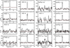 |
Fig. 6 Individual lines observed with IRAM-30m in comet C/2022 E3 during 3–6 February 2023 (average intensity, excluding offset positions). The vertical axis is main beam brightness temperature in K. The horizontal axis is the Doppler velocity in the rest frame of the comet with respect to the line. A galactic contamination of CO has been blanked out. The position and relative intensity of the hyperfine components of the HCN(3–2), HCN(2–1), and H13CN(3–2) lines have been drawn below the lines. |
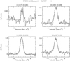 |
Fig. 7 Selected averages of the OH lines observed at the NRT in comet C/2021 A1 (Leonard) in November-December 2021 (averages of the 1667 and 1665 MHz lines scaled to 1667 MHz). |
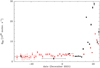 |
Fig. 8 Time evolution of comet C/2021 A1 (Leonard), single days, and averages of selected periods in November-December 2021. The OH production rates from the NRT are plotted in black. The daily water production rates inferred from SOHO/SWAN observations of the wide H Lyman-α coma, which tends to smooth out short term variations, are plotted in red. (Combi et al. 2023a). |
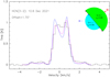 |
Fig. 9 Average spectrum of the HCN(3–2) line observed from 8.5 to 13.4 December in comet C/2021 A1, with simulated profiles. The model in blue assumes a production rate of 2.1 × 1025 molecules s−1 at 0.88 km s−1 on the sunward hemisphere and 1.1 × 1025 molecules s−1 at 0.58 km s−1 on the opposite hemisphere mostly facing the observer. The mean phase angle is ~140°, and the tilt of 40°(or 140°) with respect to the comet-observer line of sight is taken into account in this 3D simulation, as depicted in the upper right. The model in purple uses variable velocities in both hemispheres (see text), with production rates of 2.3 × 1025 molecules s−1 and 0.9 × 1025 molecules s−1, respectively. The vertical axis is main beam brightness temperature in K. The horizontal axis is the Doppler velocity in the rest frame of the comet. |
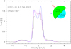 |
Fig. 10 Average FTS spectrum of the HCN(3–2) line observed from 3.7 to 6.7 February in comet C/2022 E3 with simulated profiles. The model in blue assumes a production rate of 3.0 × 1025 molecules s−1 at 0.76 km s−1 on the sunward hemisphere and 1.5 × 1025 molecules s−1 at 0.52 km s−1 on the other hemisphere, as depicted in the upper right. The model in purple uses variable velocities in both hemispheres (see text), with production rates of 3.0 × 1025 molecules s−1 and 1.0 × 1025 molecules s−1, respectively. The mean phase angle is ~45°. The vertical axis is main beam brightness temperature in K, and the horizontal axis is Doppler velocity in the rest frame of the comet. |
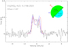 |
Fig. 11 Average spectrum of the CH3OH line at 266.838 GHz observed from 3.7 to 6.7 February 2023 in comet C/2022 E3 at the same time as HCN(3–2). The model in blue assumes a production rate of 5.6 × 1026 molecules s−1 at 0.76 km s−1 on the sunward hemisphere and 2.8 × 1026 molecules s−1 at 0.52 km s−1 on the other hemisphere, as depicted in the upper right, while the red profile comes from symmetric outgassing at 0.68 km s−1 and same total production rate (8.4 × 1026 molecules s−1). The model in purple uses the same variable velocities in both hemispheres as in Fig. 10, with production rates of 6.4 × 1025 molecules s−1and 2.0 × 1025 molecules s−1, in sunward and other hemispheres, respectively. The mean phase angle is ~45°. The vertical axis is main beam brightness temperature in K, and the horizontal axis is Doppler velocity in the rest frame of the comet. |
Rotational temperatures and inferred gas kinetic temperatures.
4 Production rates and abundances
Production rates are computed using our excitation and radiative transfer codes, and parameters as in previous papers (Biver et al. 2021a). We assumed isotropic outgassing and a constant velocity and temperature (Sects. 3.1 and 3.2). We provide both daily production rates when the molecules are detected with a sufficiently high signal-to-noise (Tables B.1 and B.2) and averages over the 13–16 November and 8–13 December 2021 periods for comet C/2021 A1 (Leonard) and 3–7 February 2023 for comet C/2022 E3 (ZTF) (Tables B.3 and B.4). For the molecules for which we observed several lines ‘i’, either detected individually with a S/N >5 or not, the final production rate is the weighted average of all production rates Qi. They are computed on each considered line (even when Qi is negative) and averaged with weighting according to 1/σ(Qi)2 were σ(Qi) is the uncertainty in production rate deduced from the line ‘i’.
4.1 Reference water production rate
Water production rates are inferred from the monitoring of OH lines at 18-cm with the NRT (Sec. 2.4) and H2O observations at 557 GHz with Odin (Sec. 2.2). Water productions rates for these comets were also obtained from SOHO/SWAN (Combi et al. 2023a,b). For the period of observations with the IRAM-30m radio telescope, and to compute relative abundances, we estimate ![$\[Q_{\mathrm{H}_2 \mathrm{O}}=2,3\]$](/articles/aa/full_html/2024/10/aa50921-24/aa50921-24-eq1.png) , and 4×1028 molecules s−1 for the 12, 13–16 November, and 8–13 December 2021, respectively, for comet C/2021 A1 (Leonard). For comet C/2022 E3 (ZTF), extrapolation from Odin production rates in Table 2, following
, and 4×1028 molecules s−1 for the 12, 13–16 November, and 8–13 December 2021, respectively, for comet C/2021 A1 (Leonard). For comet C/2022 E3 (ZTF), extrapolation from Odin production rates in Table 2, following ![$\[1 / r_h^2\]$](/articles/aa/full_html/2024/10/aa50921-24/aa50921-24-eq2.png) , yields
, yields ![$\[Q_{\mathrm{H}_2 \mathrm{O}}=5 \times 10^{28}\]$](/articles/aa/full_html/2024/10/aa50921-24/aa50921-24-eq3.png) molecules s−1 for the 3–7 February period. These values also follow the longer term trend of brightness evolution. We use these values to determine collisional rates and abundances relative to water.
molecules s−1 for the 3–7 February period. These values also follow the longer term trend of brightness evolution. We use these values to determine collisional rates and abundances relative to water.
4.2 Temporal variations in the production rates
Evidence for short-term variability in the outgassing is present both in Odin and IRAM data for comet C/2022 E3 (ZTF), but not for comet C/2021 A1. Visual inspection of the production rates folded on a single period seems to indicate a periodic pattern of about 0.35 days in ![$\[Q_{\mathrm{H}_2 \mathrm{O}}\]$](/articles/aa/full_html/2024/10/aa50921-24/aa50921-24-eq4.png) and 0.38 days in
and 0.38 days in ![$\[Q_{\mathrm{CH}_3 \mathrm{OH}}\]$](/articles/aa/full_html/2024/10/aa50921-24/aa50921-24-eq5.png) while optical observations have reported a periodic pattern in the CN structures of 0.363 ± 0.004 days (Knight et al. 2023) and 0.354 ± 0.004 days (Manzini et al. 2023). We fitted (Figs. 12 and 13) a sine-wave variation (for simplicity – a more complex profile would require more parameters) to our water and methanol production rates and found similar periods. Table 2 provides the fitted parameters and their uncertainty based on χ2 minimisation for a simple sinusoidal pattern. The relative amplitudes are 18% for methanol and 5% for H2O. H2O being observed with a beam about ten times larger (the Odin beam radius of 33000 km covers molecules emitted over a full period of 0.38 days), and having optically thick lines, it is expected to display shallower variations. The amplitude of the variations for production rate of methanol are more likely to represent the full extent of variations of outgassing of the nucleus and are similar to the variations (±20%) observed for HCN. This has to be taken into account when deriving precise ratios (e.g. isotopic ratios in Sec. 4.6), but for general abundances averaged over the four days the impact is small, especially as on the 4, 5, and 6 February evenings (Table A.2) the observations covered more than a full period of ~0.36 days.
while optical observations have reported a periodic pattern in the CN structures of 0.363 ± 0.004 days (Knight et al. 2023) and 0.354 ± 0.004 days (Manzini et al. 2023). We fitted (Figs. 12 and 13) a sine-wave variation (for simplicity – a more complex profile would require more parameters) to our water and methanol production rates and found similar periods. Table 2 provides the fitted parameters and their uncertainty based on χ2 minimisation for a simple sinusoidal pattern. The relative amplitudes are 18% for methanol and 5% for H2O. H2O being observed with a beam about ten times larger (the Odin beam radius of 33000 km covers molecules emitted over a full period of 0.38 days), and having optically thick lines, it is expected to display shallower variations. The amplitude of the variations for production rate of methanol are more likely to represent the full extent of variations of outgassing of the nucleus and are similar to the variations (±20%) observed for HCN. This has to be taken into account when deriving precise ratios (e.g. isotopic ratios in Sec. 4.6), but for general abundances averaged over the four days the impact is small, especially as on the 4, 5, and 6 February evenings (Table A.2) the observations covered more than a full period of ~0.36 days.
For other species day-to-day variations of the production rates are provided in Tables B.1 and B.2, and plotted in Figs. 14 and 15, together with some estimates of the Afρ quantity8 in order to have a rough idea of the relative evolution of the dust production rate.
4.3 Molecules coming from a distributed source
The coarse mapping done during the observations provides some information on the spatial extent of the emission for some molecules, within 14″ from the nucleus (2400 km at the distance of comet C/2021 A1 in December 2021) to ~20″ (4500 km) for comet C/2022 E3 (ZTF). Tables B.5 and B.6 provide information on the spatial extent of the emission of some molecules (average line intensities as a function of pointing offset) and constraints on the scale length and production from a distributed source. We adjusted a Haser daughter species density profile to the data and provide the result of the χ2 minimisation with 1σ uncertainty on the scale length (Lp) and production rate (Qp). Values for other fixed scale lengths (Qp and corresponding χ2) are provided. These results have to be taken with caution since: (i) the excitation of the rotational levels is not perfectly known due to variable temperature in the coma, unknown collisional cross-sections, and other poorly estimated processes that can mimic extended emission, (ii) the comet was variable in activity (it underwent a huge outburst on 14 December just after the last observation), (iii) the observations are mostly probing the 1600–5000 km spatial scales (beam size – extent of the mapping), so that information on very different scale lengths is not well constrained.
HCN: it has been shown to be mostly released from nucleus ices (Cordiner et al. 2014), but the IR observations (Dello Russo et al. 2016; Lippi et al. 2021) that probe the inner part of the coma also generally find higher production rates of HCN than the radio ones (Biver et al. 2024). The observations of both comets (data were treated day by day to limit time variability effects) suggest that a fraction of HCN is produced in the coma. The best fit to the 12.5 and 13.4 December observations of comet C/2021 A1 yield a parent scale length of the order of 350 km with Qp(HCN) larger by 15 to 35% than with Lp = 0. HCN(3–2) data from comet C/2022 E3 (ZTF) yield a scale length of 600 ± 500 km while HCN(2–1) suggest Lp(HCN) < 780 km, implying also Qp(HCN) larger by ≈20% (Tables B.5 and B.6). In both comets the retrieved parent scale length is smaller than the beam size, so the extended production of HCN needs to be further investigated at higher spatial resolution. The retrieved production rate would only be increased by ≈20%, but other issues show that the excitation of HCN is not fully understood. We also cannot exclude that an excitation process, for example a larger gas temperature or electron collision rate that would decrease the J=3 rotational level population close to the nucleus, is responsible for this apparent distributed production. Also the imperfect modelling of the line shape (underestimation of the J(3–2) F = 2–2 and F = 3–3 hyperfine satellite lines and a signal strength around zero velocity in Figs. 9, 10 being too high), suggest that there are other issues. A much larger opacity could provide a better fit to the line shape, although requiring unrealistic production rate and line intensity.
HNC: the mean of offset observations of HNC(3–2) on the whole period does not yield a significant detection (signal-to-noise is below 2) but Lp = 0 ± 700 km from χ2 minimisation is the best fit to comet C/2021 A1 data. In comet C/2022 E3 we find Lp > 2800 km at 1-σ, also poorly constrained with signal below 3-σ at offsets larger than 5″. Interferometric observations of HNC (Cordiner et al. 2017; Roth et al. 2021) suggest a parent scale length of the order of ~2000 km at 1 au (scaled as ![$\[r_h^{-2}\]$](/articles/aa/full_html/2024/10/aa50921-24/aa50921-24-eq9.png) ), somewhat compatible with our data. Therefore, we provide in the tables Qp(HNC) for nuclear source Lp = 0 and Lp(HNC) = 1000 km and 2000 km for comets C/2021 A1 and C/2022 E3, respectively.
), somewhat compatible with our data. Therefore, we provide in the tables Qp(HNC) for nuclear source Lp = 0 and Lp(HNC) = 1000 km and 2000 km for comets C/2021 A1 and C/2022 E3, respectively.
CS: in comet Leonard we obtained data at offset positions on three different dates: 10.5, 12.5, and 13.6 December. The only two points obtained on the first date do not yield significant constraints (Lp(CS) > 800 km at 1σ) and are not listed in Table B.5. The larger dataset of J=5–4 line observations of 12.48 December (Table B.5) yields a reliable value (reduced ![$\[\chi_\nu^2=0.94\]$](/articles/aa/full_html/2024/10/aa50921-24/aa50921-24-eq10.png) ): Lp(CS) =
): Lp(CS) = ![$\[500_{-390}^{+580}\]$](/articles/aa/full_html/2024/10/aa50921-24/aa50921-24-eq11.png) . We tried to combine the J=5–4 and J=3–2 observations of 13.6 December but they yield a large value for Lp(CS) > 2700 km (mostly driven by the CS(5–4) data that yield Lp(CS) > 2400 km at 1σ). This implies a too large value Qp(CS) = 12.6 × 1025 molecules s−1 for the nominal fitted value of Lp(CS) = 7000 km. Since CS(3–2) and CS(5–4) were not observed simultaneously, the constraint may not be reliable. CS(3–2) data taken alone suggests Lp(CS) ~ 1400 km, with Qp(CS) = 5.2 × 1025 molecules s−1 although compatible with any value of Lp at 1σ.
. We tried to combine the J=5–4 and J=3–2 observations of 13.6 December but they yield a large value for Lp(CS) > 2700 km (mostly driven by the CS(5–4) data that yield Lp(CS) > 2400 km at 1σ). This implies a too large value Qp(CS) = 12.6 × 1025 molecules s−1 for the nominal fitted value of Lp(CS) = 7000 km. Since CS(3–2) and CS(5–4) were not observed simultaneously, the constraint may not be reliable. CS(3–2) data taken alone suggests Lp(CS) ~ 1400 km, with Qp(CS) = 5.2 × 1025 molecules s−1 although compatible with any value of Lp at 1σ.
In comet C/2022 E3, taken separately, CS(3–2) and CS(5–4) maps yield parent scale lengths of Lp(CS) = ![$\[1400_{-930}^{+2000}\]$](/articles/aa/full_html/2024/10/aa50921-24/aa50921-24-eq12.png) and
and ![$\[700_{-620}^{+1450} \mathrm{km}\]$](/articles/aa/full_html/2024/10/aa50921-24/aa50921-24-eq13.png) , or Lp(CS) =
, or Lp(CS) = ![$\[1900_{-570}^{+900}\]$](/articles/aa/full_html/2024/10/aa50921-24/aa50921-24-eq14.png) combining all data (larger since constrained by a unique value for Qp(CS), Table B.6).
combining all data (larger since constrained by a unique value for Qp(CS), Table B.6).
Around these heliocentric distances (0.8 and 1.2 au), the CS2 photo-dissociation scale lengths are expected to be ~260 and 560 km. The average of all measurements obtained, yield Lp(CS) >800 and 1300–2200 km, respectively. Most other observations also suggest a parent scale length for CS that is about 3–5 times the CS2 dissociation scale length (Biver et al. 2022; Roth et al. 2021). Hence, we use Lp(CS)=1000 and 2000 km for C/2021 A1 and C/2022 E3, respectively. This is equivalent to assuming that CS comes from a parent molecule X-CS with a photo-dissociation rate at 1 au β0(X − CS) ~ 4.5 × 10⁻⁴ s−1, which is comparable to the revised photo-destruction rate of H2CS (β0(H2CS) = 4.9 × 10⁻⁴ s−1, Hrodmarsson & van Dishoeck 2023). However upper limits on the H2CS abundance are much lower than for CS parent. We note that assuming that CS comes directly from the nucleus reduces the production rate by only ~14% when comparing to the case of production by dissociation of CS2 with its known lifetime.
H2CO: combining the two ![$\[J_{K_a K_c}=3_{1 K_c}\]$](/articles/aa/full_html/2024/10/aa50921-24/aa50921-24-eq15.png) lines at 211.211 and 225.698 GHz observed on 12.6 December provides some constraints on the spatial distribution of H2CO in the coma of comet C/2021 A1. The retrieved parent scale length is
lines at 211.211 and 225.698 GHz observed on 12.6 December provides some constraints on the spatial distribution of H2CO in the coma of comet C/2021 A1. The retrieved parent scale length is ![$\[1500_{-970}^{+3700}\]$](/articles/aa/full_html/2024/10/aa50921-24/aa50921-24-eq16.png) (Table B.5) within the range of values (0.2–1.6× the photo-destruction scale length Ld of H2CO, which is 2200 km around 12 December), found from previous observations (Biver et al. 2022, 1999; Roth et al. 2021; Cordiner et al. 2014). The +1σ uncertainty is large and the upper limit not very precise (χ2 does not increase as steeply as for the lower limit). In addition, if there is some nucleus contribution, we can mostly say that the H2CO coming from a distributed source must have a parent scale length larger than 1400 km. We use Lp(H2CO) = 1500 and 2800 km (0.68 × Ld(H2CO)) to retrieve the (parent) production rate of H2CO in December and November, respectively.
(Table B.5) within the range of values (0.2–1.6× the photo-destruction scale length Ld of H2CO, which is 2200 km around 12 December), found from previous observations (Biver et al. 2022, 1999; Roth et al. 2021; Cordiner et al. 2014). The +1σ uncertainty is large and the upper limit not very precise (χ2 does not increase as steeply as for the lower limit). In addition, if there is some nucleus contribution, we can mostly say that the H2CO coming from a distributed source must have a parent scale length larger than 1400 km. We use Lp(H2CO) = 1500 and 2800 km (0.68 × Ld(H2CO)) to retrieve the (parent) production rate of H2CO in December and November, respectively.
For comet C/2022 E3 (Table B.6), we made observations at offset positions up to 20″ on 5.00 February and 28″ on 5.95 February (4400–6500 km with a 2400 km beam) that provide more stringent constraints on the spatial distribution of H2CO. For the assumed Haser daughter distribution profile, we found Lp(H2CO) = 1000 ± 430 and 1700 ± 1100 km, respectively. The observations of 6.94 February as well as those obtained for other lines (211 − 110 line at 150.498 GHz) provide looser constraints that fully encompass those values. Fig. 16 shows the combination of all H2CO observations at 211 and 226 GHz in comet C/2022 E3 versus expected evolution of line intensity as a function of pointing offset for various parent scale lengths – the retrieved Lp(H2CO) is 1700 ± 500 km which corresponds to 0.36 ± 0.11 × Ld(H2CO) at 1.18 au from the sun, with vexp = 0.68 km s−1.
NH2CHO and CH3CHO: we have also studied the spatial distribution of these two species (only NH2CHO in C/2021 A1): results are not conclusive and may be affected by excitation effects (especially for the high Ka transitions of formamide). Slightly distributed production (with Lp ~ 1500 km) could be favoured for comet C/2022 E3, but a nuclear source is not clearly excluded (within the 2 − σ uncertainty) as for formaldehyde.
In addition, if a significant production of the molecules comes from the sublimation of icy grains in the coma, all species could also show some distributed production. But the least distributed species like HCN, could put an upper limit on the spatial extent of the distributed production. The production of CS and H2CO remains clearly more distributed and they are thus daughter products.
Time periods found to fit comet C/2022 E3 (ZTF) production rates.
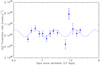 |
Fig. 12 Water production rates (in molecules s−1) of comet C/2022 E3 (ZTF) between 19.3 and 20.3 January 2023 derived from observations with Odin (central pointings). A best fit sinusoidal variation is plotted in blue. |
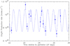 |
Fig. 13 Methanol production rates (in molecules s−1) of comet C/2022 E3 (ZTF) between 3.7 and 7.1 February 2023 derived from observations with IRAM 30m. An average 5% calibration uncertainty has been added to the formal uncertainty due to system temperature noise. A best fit sinusoidal variation is plotted in blue. |
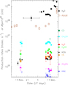 |
Fig. 14 Production rates of comet C/2021 A1 (Leonard) in November and December 2021. Water production rates are 1.1 × QOH from Sec. 2.4. Afρ were measured from images of the comet by N. Biver, not corrected for the phase angle. |
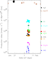 |
Fig. 15 Production rates of comet C/2022 E3 (ZTF) in January and February 2023. Water production rates are from Odin observations (Sec. 2.2, Fig. 12). We note that Afρ(0°) were measured from images of the comet by N. Biver and have been corrected for the phase angle. |
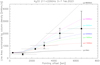 |
Fig. 16 Spatial distribution of formaldehyde in comet C/2022 E3 (ZTF). This plot shows for the average of all observations of the twin 211 GHz and 226 GHz lines observed together in comet C/2022 E3 (ZTF) from 3 to 7 February 2023: (i) in black squares (with error-bars) the observed line integrated intensity, (ii) in solid and dotted lines the expected intensity for parent scale length of 0 or 1000–8000 km. For better visibility a normalisation has been applied: at each offset the line intensity is multiplied by the column density at the first offset divided by the one expected at the considered offset point, for a parent distribution. Production rate of the models are adjusted to get the same integrated intensity at the first point. Deviation from a flat line for Lp = 0 (black continuous line) is due to excitation effects. Vertical axis is normalised integrated intensity in mK km/s and horizontal axis is pointing offset converted into km at the distance of the comet. |
4.4 Relative abundances
Abundances relative to water, assuming ![$\[Q_{\mathrm{H}_2 \mathrm{O}}=2{-}3 \times 10^{28}\]$](/articles/aa/full_html/2024/10/aa50921-24/aa50921-24-eq17.png) molecules s−1 in November and
molecules s−1 in November and ![$\[Q_{\mathrm{H}_2 \mathrm{O}}=4 \times 10^{28}\]$](/articles/aa/full_html/2024/10/aa50921-24/aa50921-24-eq18.png) molecules s−1 in December 2021 for comet C/2021 A1 and
molecules s−1 in December 2021 for comet C/2021 A1 and ![$\[Q_{\mathrm{H}_2 \mathrm{O}}=5 \times 10^{28}\]$](/articles/aa/full_html/2024/10/aa50921-24/aa50921-24-eq19.png) molecules s−1 in early February 2023 for comet C/2022 E3 are provided in Table 3. Abundances have also been measured for several molecules in comet C/2021 A1 in the infrared by Faggi et al. (2023), but during the outbursting period of the comet in December-January. While these authors found very similar abundances for HCN, OCS, H2CO, and compatible with our upper limit on CO, they did not detect CH3OH. Their inferred CH3OH/H2O is very low, down to one order of magnitude lower than our abundance (based on the secure detection of over 42 lines). Either the comet had exhausted its methanol content during the outburst phase at the end of December, or the infrared observations missed part of the methanol emission, following a trend also seen in millimetre investigations (Biver et al. 2011) which show an apparent decrease in methanol abundance as comets get closer to the Sun. The methanol observations of Faggi et al. (2023) were obtained at 0.62 au from the Sun, where the sampled gas coma gets warmer (assumed to be 120 K) and the fraction of methanol in an excited torsional state may also depopulate the ground vibrational levels.
molecules s−1 in early February 2023 for comet C/2022 E3 are provided in Table 3. Abundances have also been measured for several molecules in comet C/2021 A1 in the infrared by Faggi et al. (2023), but during the outbursting period of the comet in December-January. While these authors found very similar abundances for HCN, OCS, H2CO, and compatible with our upper limit on CO, they did not detect CH3OH. Their inferred CH3OH/H2O is very low, down to one order of magnitude lower than our abundance (based on the secure detection of over 42 lines). Either the comet had exhausted its methanol content during the outburst phase at the end of December, or the infrared observations missed part of the methanol emission, following a trend also seen in millimetre investigations (Biver et al. 2011) which show an apparent decrease in methanol abundance as comets get closer to the Sun. The methanol observations of Faggi et al. (2023) were obtained at 0.62 au from the Sun, where the sampled gas coma gets warmer (assumed to be 120 K) and the fraction of methanol in an excited torsional state may also depopulate the ground vibrational levels.
4.5 Upper limits
The surveys cover part of the 2 mm wavelength range and most of the 1 mm (210–272 GHz) as shown in spectra online. Most of the known organic molecules have many transitions in these wavelength ranges. We have not noticed clearly unidentified lines (above the 5 − σ level). We checked the sensitivity of the observations for the following molecules: CH3SH, CH3OCH3, CH3COCH3, c-C2H4O, c-C3H2, CH3NH2, C2H3CN, CH3Cl, and propanal. Averaging the lines expected to be the strongest did not yield any significant signal. 3 − σ upper limits on abundances and production rates are provided in Tables 3, B.3, and B.4, and for the species not listed the upper limits on abundances are not expected to be better than in previous comets such as 46P/Wirtanen (Biver et al. 2021a).
4.6 Isotopic ratios
Isotopic ratios of H, C, N, and S and upper limits on their abundances in some molecules are provided in Table 4. Regarding HCN isotopologues, none are clearly detected but upper limits or marginal signal at the 2–3-σ level are compatible with values observed in other comets (Biver et al. 2024). Note that for 15N/14N, the Earth value of 272 corresponds already to an enrichment compared to the estimated solar value of 450 (Marty et al. 2011), showing that fractionation was important already for Earth nitrogen but even more for the material that was incorporated into cometary ices 4.5 billion years ago.
The 32S/34S could be measured in CS in both comets, but in comet C/2022 E3 it seems lower than the Earth value while compatible with terrestrial value for H2S: this comet seems enriched in C34S, at the 3-σ level. However the PSW observing mode used for comet C/2022 E3 is more prone to produce ripples that affect the signal of marginal lines. We also provide upper limits on abundances of deuterated species. None yields a D/H below the Earth VSMOW (Vienna Standard Mean Ocean Water) value, but since some enrichment has been observed in the interstellar medium and in some molecules ejected by comet 67P/Churyumov-Gerasimenko observed by the ROSINA mass spectrometer on board the Rosetta spacecraft (Drozdovskaya et al. 2021; Müller et al. 2022), we provide those upper limits.
5 The abundance of HNCO and HCOOH in comets
The molecules HNCO and HCOOH were first detected in comets C/1996 B2 (Hyakutake) and C/1995 O1 (Hale-Bopp) in 1996–1997 (Lis et al. 1997; Bockelée-Morvan et al. 2000). They have been detected in several comets since (Biver et al. 2023a) but there were large uncertainties on their destruction rates and lifetimes and a simple excitation model was used to derive their abundances. Hrodmarsson & van Dishoeck (2023) have recently published photo-dissociation and photo-ionisation rates for HNCO and HCOOH that significantly differ from those assumed in the past (Biver et al. 2021a, and references therein). The new values (β0(HNCO) = 38 × 10−5 s−1, β0(HCOOH) = 54 × 10−5 s−1, in the solar radiation field at 1 au) are 5 to 10 times higher than previously assumed, with a stated 2-σ uncertainty of the order of 20–30% (Hrodmarsson & van Dishoeck 2023). We have decided to revisit all millimetre observations of comets reporting a detection of at least one of these molecules and recomputed production rates and abundances relative to water assuming values of:
β0(HNCO) = 3.5 × 10⁻⁴ s−1;
β0(HCOOH) = 5.0 × 10⁻⁴ s−1.
The contribution of Solar Lyman-α to their photo-dissociation is minor and their photo-dissociation cross-section extends well into the 130–200 nm range where the solar flux is less affected by solar activity (Huebner et al. 1992). Therefore, we do not expect a large variation with solar activity. An overview of the observations analysed in this work, partly published in previous papers is given in Table A.3.
Table 5 provides the abundances relative to water of HNCO and HCOOH in these comets. In these calculations infrared pumping via the rotational bands is not taken into account, but with those reduced lifetimes, the photo-dissociation of the molecules takes place in a region where collisional excitation dominates (within ~2000 km from the nucleus) and the photo-dissociation process is as efficient as vibrational excitation (g-factors comparable to β). So the new reduced lifetimes (compared to previous calculations) should also reduce the uncertainties from the neglected infrared pumping.
HNCO is relatively well detected in the two comets via its Ka = 0 lines at 2 mm and 1 mm wavelengths, and marginal signals at an offset of 10″ (Tables B.5, B.6) suggest that it may be produced by a distributed source with a scale length Lp(HNCO) larger than 2000 km. Indeed, assuming a parent scale length of 5000 km also provides a better agreement between the observed rotational temperature and the predicted one for T = 60 K (Table 1).
HCOOH: In Tables B.5 and B.6 we have selected the lower energy lines that are expected to be the strongest, that is those with Ka = 0 to 2. For comet C/2021 A1, since at the offset position the weighted average intensity is similar to the one at the central position, we do not find a solution for a reasonably small parent scale length, but data are compatible within 1σ with Lp(HCOOH) = 2000 km, and Lp(HCOOH) = 0 km cannot be fully excluded. Similarly, for comet C/2022 E3, we derive Lp(HCOOH) = 0–5200 km in the ±1σ interval, so that distributed source as well as nuclear source are not excluded. Hence, if HCOOH is produced by the sublimation and dissociation of ammonium formate, then this must take place within a few thousands of kilometers from the nucleus at 0.78–1.18 au from the Sun.
The revised measured abundances in comets (increased by a factor 1.2 to 5) of these two molecules are plotted in Fig. 17 as a function of heliocentric distance at which they were detected. This plots suggest that their abundance relative to water increases for comets observed closer to the Sun. This needs to be confirmed, but can suggest that the molecules could be at least in part produced by the degradation of parents in the coma such as ammonium salts. Their combined abundance relative to water in comets (~0.1–1%) is comparable to that of NH3(0.2–5%, Biver et al. 2024), the other decomposition product of ammonium salts. Interestingly, a similar trend with heliocentric distance has been observed for the abundance of ammonia (see, e.g. Dello Russo et al. 2016).
Molecular abundances.
Isotopic ratios.
Revised abundances of HNCO and HCOOH in comets.
6 Conclusions
We have undertaken a comprehensive and sensitive spectroscopic survey at 2 mm and 1 mm of two long period comets, C/2021 A1 (Leonard) and C/2022 E3 (ZTF) when they were relatively close to the Earth (0.2–0.3 au). We collected in addition some useful spatial information from coarse mapping, to probe the spatial distribution of selected molecules. The main results can be summarised as follows:
Both comets exhibited relatively stable (within ±20%) production rates during the observational periods, although C/2021 A1 underwent a series of disintegration outbursts just after our IRAM-30m observing run;
We determined the abundance relative to water or a significant upper limit for 26 molecules. Comets C/2021 A1 and C/2022 E3 share similar compositions: they are depleted in hypervolatiles (low CO and H2S abundances relative to water) and have a relatively low methanol abundance relative to water (0.9 and 1.8% respectively) compared to the mean of other comets;
Constraints on the presence of distributed sources have been obtained. A slightly distributed source (scale length smaller than 1/3 beam) for HCN fits better the data than direct release from the nucleus. The parent source of formaldehyde was found to have a scale length Lp(H2CO) = 0.68 and 0.36 ± 0.11 times the photo-dissociation length of formaldehyde (Ld(H2CO)) in C/2021 A1 and C/2022 E3 respectively. We measured Lp(CS) ≈ 4 × Ld(CS2), suggesting that the dissociation rate of the parent producing CS is β0 = 4.5 × 10⁻⁴ s−1 at 1 au from the Sun. This is comparable to the photo-dissociation rate of H2CS, but the H2CS upper limit is more than 3 times lower than the CS abundance;
Both comets are relatively depleted in sulphur-bearing species compared to other comets, with H2S/H2O in the low range (0.15–0.18%) and the sum of sulphur-bearing molecule abundances below ~0.5%. SO and SO2 are not detected with abundances below the lowest measured in a comet and OCS is detected in both comets but with a low abundance, too;
We obtained only shallow constraints on isotopic ratios: 12C/13C, 14N/15N, and 32S/34S are compatible with values observed in other comets (90, 150, and 23, respectively), although the C32S/C34S seems marginally twice lower than the terrestrial value in comet C/2022 E3;
HNCO and HCOOH are well detected in both comets. Because of recently published lifetimes for these molecules that are significantly shorter than previous estimates, we have revised their inferred abundances in all comets for which detections of these species have been reported. The values found in C/2021 A1 (0.07% and 0.19%) and C/2022 E3 (0.04% and 0.19%) are close to their median abundances relative to water in other comets, 0.05% and 0.25%, respectively. Their total abundance is also about half the median abundance of NH3 in comets. We cannot exclude that these species are produced in the coma by a distributed source, and their abundance in the comae seems to increase at lower heliocentric distances. This favours the hypothesis that HNCO, HCOOH, and consequently an important fraction of NH3 could come from the decomposition of ammonium salts.
These observations have provided complementary and new insights regarding the source of several cometary molecules that are unlikely present as such in cometary ices. Further investigations at higher spatial resolution (e.g. interferometric investigations undertaken on those comets under reduction or on future comets), will be very useful to pin down the production processes and the scale lengths of these molecules (CS, H2CO, HNCO, HCOOH).
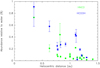 |
Fig. 17 Abundances relative to water of HNCO (green) and HCOOH (blue) in comets as a function of the heliocentric distance. Even though there is dispersion between comets, the trend appears to be that these species are more abundant in the coma close to the Sun. |
Data availability
The radio spectra are available at the CDS via anonymous ftp to cdsarc.cds.unistra.fr (130.79.128.5) or via https://cdsarc.cds.unistra.fr/viz-bin/cat/J/A+A/690/A271. The tables of line intensities are available at https://doi.org/10.5281/zenodo.13332037. The spectra of comets are available at https://doi.org/10.5281/zenodo.13341404.
Acknowledgements
This work is based on observations carried out under projects number 001-21, 100-21, and 097-22 with the IRAM 30-m telescope. IRAM is supported by the Institut Nationnal des Sciences de l’Univers (INSU) of the French Centre national de la recherche scientifique (CNRS), the Max-Planck-Gesellschaft (MPG, Germany) and the Spanish IGN (Instituto Geográfico Nacional). We gratefully acknowledge the support from the IRAM staff for its support during the observations. The data were reduced and analysed thanks to the use of the GILDAS, class software (https://www.iram.fr/IRAMFR/GILDAS). This research has been supported by the Programme national de planétologie de l’Institut des sciences de l’univers (INSU). The Nançay radio telescope (NRT) is part of the Observatoire radioastronomique de Nançay, operated by the Paris Observatory, associated with the French Centre national de la recherche scientifique (CNRS) and with the University of Orléans. Part of this research was carried out at the Jet Propulsion Laboratory, California Institute of Technology, under a contract with the National Aeronautics and Space Administration (80NM0018D0004). D.C.L. acknowledges financial support from the National Aeronautics and Space Administration (NASA) Astrophysics Data Analysis Program (ADAP). M.N. Drozdovskaya acknowledges the Holcim Foundation Stipend. B.P. Bonev and N. Dello Russo acknowledge support of NSF grant AST-2009398 and NASA grant 80NSSC17K0705, respectively. N.X. Roth was supported by the NASA Postdoctoral Program at the NASA Goddard Space Flight Center, administered by Universities Space Research Association under contract with NASA. M.A. Cordiner was supported in part by the National Science Foundation (under Grant No. AST-1614471). S.N. Milam and M.A. Cordiner acknowledge the Planetary Science Division Internal Scientist Funding Program through the Fundamental Laboratory Research (FLaRe) work package, as well as the NASA Astrobiology Institute through the Goddard Center for Astrobiology (proposal 13-13NAI7-0032).
Appendix A Additonal material
Log of observations of comet C/2021 A1 (Leonard) in 2021.
Log of observations of comet C/2022 E3 (ZTF) in 2023.
Observations of HNCO and HCOOH in comets.
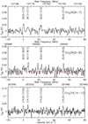 |
Fig. A.1 CH3CN series of four lines observed with IRAM-30m in comet C/2021 A1 on 8–13 December 2021 (average intensity). The vertical axis is main beam brightness temperature in K, horizontal axis is Doppler velocity in the rest frame of the comet with respect to the (J, 0) − (J − 1, 0) line, with frequencies in the rest frame of the comet given on the upper axis. |
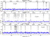 |
Fig. A.2 CH3OH series of lines around 166, 242, and 252 GHz observed with IRAM-30m in comet C/2021 A1 on 8–13 December 2021 (average intensity). The vertical axis is main beam brightness temperature in K, horizontal axis is Doppler velocity in the rest frame of the comet with respect to the main line, with frequencies in the rest frame of the comet given on the upper axis. |
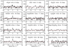 |
Fig. A.3 Spectra of molecules obtained by averaging several lines observed with IRAM-30m in comet C/2021 A1 between 8 and 13 December 2021. The vertical axis is main beam brightness temperature in K. The horizontal axis is the Doppler velocity in the rest frame of the comet. The number of lines averaged is provided for each molecule, either in the 2 mm band (147–153 and 163–171 GHz) or 1 mm band (209–272 GHz). |
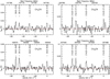 |
Fig. A.4 CH3CN series of lines at 147, 165, 220, and 257 GHz observed with IRAM-30m in comet C/2022 E3 on 3–6 February 2023 (average intensity). The vertical axis is main beam brightness temperature in K. The horizontal axis is the Doppler velocity in the rest frame of the comet with respect to the main line, with frequencies in the rest frame of the comet given on the upper axis. |
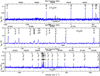 |
Fig. A.5 CH3OH series of lines around 165, 242, and 252 GHz observed with IRAM-30m in comet C/2022 E3 on 3–6 February 2023 (average intensity). The vertical axis is main beam brightness temperature in K. The horizontal axis is the Doppler velocity in the rest frame of the comet with respect to the main line, with frequencies in the rest frame of the comet given on the upper axis. |
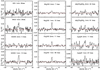 |
Fig. A.6 Spectra of molecules obtained by averaging several lines observed with IRAM-30m in comet C/2022 E3 between 3 and 6 February 2023. The vertical axis is main beam brightness temperature in K. The horizontal axis is the Doppler velocity in the rest frame of the comet. The number of lines averaged is provided for each molecule, either in the 2 mm band (147–155, 163–171, and 176–184 GHz) or 1 mm band (209–272 GHz). |
Appendix B Tables of production rates
Daily production rates in C/2021 A1 in November-December 2021.
Daily production rates in C/2022 E3 in February 2023.
Production rates in C/2021 A1 in November-December 2021 (weekly average).
Production rates in C/2022 E3 (ZTF) in February 2023.
Production from a distributed source based on offset pointings on comet C/2021 A1 (Leonard).
Production from a distributed source based on offset pointings on comet C/2022 E3 (ZTF).
Appendix C Rotational diagrams
The logarithm of a quantity proportional to the line intensity (line area divided by column density) is plotted against the energy of the upper level for each observed rotational transition. The upper levels of the transition are given at the top. The inverse of the slope of a fitted line provides the rotational temperature (given in pink) of the group of lines.
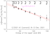 |
Fig. C.1 Rotational diagram of the CH3OH lines around 166 GHz observed between 8.6 and 13.7 December 2021 in comet C/2021 A1 (Leonard). |
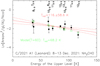 |
Fig. C.2 Rotational diagram of all the NH2CHO lines observed between 8.6 and 13.7 December 2021 in comet C/2021 A1 (Leonard). Lines with same J number and Ka = 0 to 2 or 3 to 4 are averaged together. Scales as in Fig. C.1). The values in green are those expected from modelling with T = 60 K. |
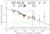 |
Fig. C.3 Rotational diagram of the CH3CN lines at 147, 165, 220, 239, and 257 GHz observed between 8.4 and 13.7 December 2021 in comet C/2021 A1 (Leonard). Scales as in Fig. C.1). The values in green are those expected from modelling with T = 60 K. |
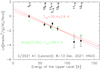 |
Fig. C.4 Rotational diagram of the HNCO lines at 1 mm and 2 mm observed between 8.4 and 13.7 December 2021 in comet C/2021 A1 (Leonard). Scales as in Fig. C.1. |
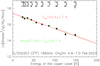 |
Fig. C.5 Rotational diagram of the CH3OH lines around 166 GHz observed between 4.9 and 7.0 February 2023 in comet C/2022 E3 (ZTF). The values in green are those expected from modelling with T = 60 K. |
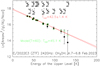 |
Fig. C.6 Rotational diagram of the CH3OH lines at 242 GHz observed between 4.7 and 6.8 February 2023 in comet C/2022 E3 (ZTF). Scales as in Fig. C.5. |
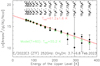 |
Fig. C.7 Rotational diagram of the CH3OH lines around 252 GHz observed between 3.7 and 6.7 February 2023 in comet C/2022 E3 (ZTF). Scales as in Fig. C.5. |
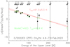 |
Fig. C.8 Rotational diagram of the CH3CN lines at 147 and 165 GHz observed between 4.9 and 7.0 February 2023 in comet C/2022 E3 (ZTF). Scales as in Fig. C.5. |
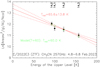 |
Fig. C.9 Rotational diagram of the CH3CN lines at 257 GHz observed between 3.7 and 6.7 February 2023 in comet C/2022 E3 (ZTF). Scales as in Fig. C.5. |
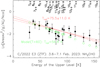 |
Fig. C.10 Rotational diagram of all the NH2CHO lines observed between 3.6 and 7.1 February 2023 in comet C/2022 E3 (ZTF) at 1 mm and 2 mm. Some lines with the same J and Ka levels (and/or similar energy levels and Einstein A coefficients) have been grouped together (Kc given as 0 in the third quantum number of the line). Scales as in Fig. C.5. |
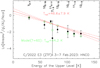 |
Fig. C.11 Rotational diagram of all the HNCO lines observed between 3.6 and 7.1 February 2023 in comet C/2022 E3 (ZTF). The lines with the same J for Ka = 1 levels have been grouped together. Scales as in Fig. C.5. |
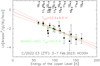 |
Fig. C.12 Rotational diagram of all the HCOOH lines observed between 3.6 and 7.1 February 2023 in comet C/2022 E3 (ZTF). Scales and grouping of lines as in Fig. C.10. |
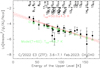 |
Fig. C.13 Rotational diagram of all the CH3CHO lines observed between 3.6 and 7.1 February 2023 in comet C/2022 E3 (ZTF). Scales and grouping of lines as in Fig. C.10. |
References
- A’Hearn, M. F., Millis, R. L., Schleicher, D. G., Osip, D.J., & Birch, P. V. 1995, Icarus, 118, 223 [CrossRef] [Google Scholar]
- Altwegg, K., & Bockelée-Morvan, D. 2003, Space Sci. Rev., 106, 139 [Google Scholar]
- Altwegg, K., Balsiger, H., Hänni, N., et al. 2020, Nat. Astron., 4, 533 [NASA ADS] [CrossRef] [Google Scholar]
- Biver, N., & Bockelée-Morvan, D. 2019, ACS Earth Space Chem., 3, 1550 [Google Scholar]
- Biver, N., Bockelée-Morvan, D., Crovisier, J., et al. 1999, AJ, 118, 1850 [NASA ADS] [CrossRef] [Google Scholar]
- Biver, N., Bockelée-Morvan, D., Crovisier, J., et al. 2002, Earth Moon Planets, 90, 323 [Google Scholar]
- Biver N., Bockelée-Morvan D., Colom P., et al. 2011, A&A, 528, A142 [NASA ADS] [CrossRef] [EDP Sciences] [Google Scholar]
- Biver, N., Moreno, R., Bockelée-Morvan, D., et al. 2016, A&A, 589, A78 [NASA ADS] [CrossRef] [EDP Sciences] [Google Scholar]
- Biver, N., Bockelée-Morvan, D., Hofstadter, M., et al. 2019, A&A, 630, A19 [NASA ADS] [CrossRef] [EDP Sciences] [Google Scholar]
- Biver, N., Bockelée-Morvan, D., Boissier, J., et al. 2021a, A&A, 648, A49 [EDP Sciences] [Google Scholar]
- Biver, N., Bockelée-Morvan, D., Lis, D. C., et al. 2021b, A&A, 651, A25 [NASA ADS] [CrossRef] [EDP Sciences] [Google Scholar]
- Biver, N., Bockelée-Morvan, D., Boissier, J., et al. 2022, A&A, 668, A171 [NASA ADS] [CrossRef] [EDP Sciences] [Google Scholar]
- Biver, N., Bockelée-Morvan, D., Crovisier, J., et al. 2023a, A&A, 670, A170 [NASA ADS] [CrossRef] [EDP Sciences] [Google Scholar]
- Biver, N., Bockelée-Morvan, D., Crovisier, J., et al. 2023b, CBET, 5216 [Google Scholar]
- Biver N., Dello Russo N., Opitom C., Rubin, M. 2024, arXiv e-prints [arXiv:2207.04800] [Google Scholar]
- Bockelée-Morvan, D., Lis, D. C., Wink, J. E., et al. 2000, A&A, 353, 1101 [Google Scholar]
- Bockelée-Morvan, D., Calmonte, U., Charnley, S., et al. 2015, Space Sci. Rev., 197, 47 [Google Scholar]
- Bockelée-Morvan, D., & Biver, N. 2017, Phil. Trans. R. Soc. A, 375, 20160252 [Google Scholar]
- Brasser, R., & Morbidelli, A. 2013, Icarus, 225, 40 [Google Scholar]
- Carter, M., Lazareff, R., Maier, D., et al. 2012, A&A, 538, A89 [NASA ADS] [CrossRef] [EDP Sciences] [Google Scholar]
- Combi, M., Mäkinen, T., Bertaux, J.-L., Quemerais, E., & Ferron, S. 2023a, Icarus, 398, 115543 [NASA ADS] [CrossRef] [Google Scholar]
- Combi, M., Mäkinen, T., Bertaux, J.-L., Quemerais, E., & Ferron, S. 2023b, DPS-EPSC, 322.04 (on-line poster) [Google Scholar]
- Cordiner, M. A., Remijan, A. J., Boissier, J., et al. 2014, ApJ, 792, L2 [NASA ADS] [CrossRef] [Google Scholar]
- Cordiner, M. A., Boissier, J., Charnley, S. B., et al. 2017, ApJ, 838, 147 [Google Scholar]
- Cordiner, M. A., Palmer, M. Y., de Val-Borro, M., et al. 2019, ApJ, 870, L26 [Google Scholar]
- Crovisier, J., Colom, P., Gérard, E., Bockelée-Morvan, D., & Bourgois, G. 2002, A&A, 393, 1053 [NASA ADS] [CrossRef] [EDP Sciences] [Google Scholar]
- Crovisier, J., Biver, N., & Bockelée-Morvan, D. 2021, CBET, 5087 [Google Scholar]
- Dello Russo, N., Kawakita, H., Vervack, R. J., & Weaver, H. A. 2016, Icarus, 278, 301 [NASA ADS] [CrossRef] [Google Scholar]
- Drozdovskaya, M. N., Schroeder, I I. R. H. G., Rubin, M., et al. 2021, MNRAS, 500, 4901 [Google Scholar]
- Faggi, S., Lippi, M., Mumma, M. J., & Villanueva, G. L. 2023, Planetary Science Journal, 4, 8 [CrossRef] [Google Scholar]
- Frisk, U., Hagström, M., Ala-Laurinaho, J., et al. 2003, A&A, 402, L27 [NASA ADS] [CrossRef] [EDP Sciences] [Google Scholar]
- Hartogh, P., Lis, D. C., Bockelée-Morvan, D., et al. 2011, Nature, 478, 218 [Google Scholar]
- Heays, A. N., Bosman, A. D., & van Dishoeck, E. F. 2017, A&A, 602, A105 [NASA ADS] [CrossRef] [EDP Sciences] [Google Scholar]
- Hrodmarsson, H. R., & van Dishoeck, E. F. 2023, A&A, 675, A25 [NASA ADS] [CrossRef] [EDP Sciences] [Google Scholar]
- Huebner, W. F., & Mukherjee, J. 2015, Planet. Space Sci., 106, 11 [Google Scholar]
- Huebner, W. F., Keady, J. J., & Lyon, S. P. 1992, Ap&SS, 195, 1 [NASA ADS] [CrossRef] [Google Scholar]
- Jehin, E., Moulane, Y., & Manfroid, J. 2021, CBET, 5087 [Google Scholar]
- Jewitt, D., Kim, Y., Mattiazzo, M., et al. 2023, AJ, 165, 122 [NASA ADS] [CrossRef] [Google Scholar]
- Knight, M. M., Holt, C. E., Villa, K. M., Skiff, B. A., & Schleicher, D. G. 2023, ATel, 15879 [Google Scholar]
- Lecacheux, A., Biver, N., Crovisier, J., et al. 2003, A&A, 402, L55 [NASA ADS] [CrossRef] [EDP Sciences] [Google Scholar]
- Lippi, M., Villanueva, G. L., Mumma, M. J., & Faggi, S. 2021, AJ, 162, 74 [NASA ADS] [CrossRef] [Google Scholar]
- Lis, D. C., Keene, J., Young, K., et al. 1997, Icarus, 130, 355 [NASA ADS] [CrossRef] [Google Scholar]
- Manzini, F., Oldani, V., Ochner, P., Bedin, L. R., & Reguitti, A. 2023, ATel, 15909 [Google Scholar]
- Marty, B., Chaussidon, M., Wiens, R. C., Jurewicz, A. J. G., & Burnett, D. S. 2011, Science, 332, 1533 [NASA ADS] [CrossRef] [Google Scholar]
- Milam, S. N., Roth, N. X., Villanueva, G. L., et al. 2023, ACM 2023, LPI Contrib. No. 2851 [Google Scholar]
- Müller, H. S. P., Schlöder, F., Stutzki, J., & Winnewisser, G. 2005, J. Mol. Struct., 742, 215 [Google Scholar]
- Müller, D. R., Altwegg, K., Berthelier, J. J., et al. 2022, A&A, 662, A69 [NASA ADS] [CrossRef] [EDP Sciences] [Google Scholar]
- O’Brien, D. P., Walsh, K. J., Morbidelli, A., Raymond, S. N., & Mandell, A. M. 2014, Icarus, 239, 74 [Google Scholar]
- Pickett, H. M., Poynter, R. L., Cohen, E. A., et al. 1998, J. Quant. Spec. Radiat. Transf., 60, 883 [Google Scholar]
- Roth, N. X., Milam, S. N., Cordiner, M. A., et al. 2021, ApJ, 921, 14 [NASA ADS] [CrossRef] [Google Scholar]
- Šimečková, M., Jacquemart, D., Rothman, L. S., Gamache, R. R., & Goldman, A. 2006, J. Quant. Spec. Radiat. Transf., 98, 130 [CrossRef] [Google Scholar]
All Tables
Production from a distributed source based on offset pointings on comet C/2021 A1 (Leonard).
Production from a distributed source based on offset pointings on comet C/2022 E3 (ZTF).
All Figures
|
Fig. 1 Coarse map of the HCN(3–2) line integrated intensity in comet C/2021 A1 on 13.4 December 2021. The beam size is 9.3″. Solar phase angle was 158.6°. The direction of the Sun (PA=193.1°) is indicated at the lower right. |
| In the text | |
|
Fig. 2 Millimetre lines observed with IRAM-30m in comet C/2021 A1 during 12–16 November 2021 (average intensity). The CH3OH line is the sum of the J=1 to 4 J1 − J0 E lines at 165050.175, 165061.130, 165099.240, and 165190.475 MHz observed with the high resolution backend VESPA. The vertical axis is main beam brightness temperature in K and the horizontal axis is Doppler velocity in the rest frame of the comet with respect to the main line. |
| In the text | |
|
Fig. 3 Individual lines observed with IRAM-30m in comet C/2021 A1 during 8–13 December 2021 (weighted averages). The vertical axis is main beam brightness temperature in K and the horizontal axis is Doppler velocity in the rest frame of the comet with respect to the line. The position and relative intensity of the hyperfine components of the HCN(3–2) line have been drawn below the line. |
| In the text | |
|
Fig. 4 Map of the average spectra of the H2O(110−101) line obtained with Odin between 19.45 and 20.16 January 2023 in comet C/2022 E3 (ZTF), as a function of the pointing offset (in arcsec). A baseline in red is plotted on each spectrum. Solar phase angle was 61.6°, and the direction of the Sun (PA=120.2°) is indicated at the upper right with scales for individual AC2 spectra. |
| In the text | |
|
Fig. 5 Coarse (3×3 points) map of the HCN(3–2) line integrated intensity on 4.67 February 2023 in comet C/2022 E3. Solar phase angle was 45.5°. The direction of the Sun (PA=287°) is indicated at the upper right. |
| In the text | |
|
Fig. 6 Individual lines observed with IRAM-30m in comet C/2022 E3 during 3–6 February 2023 (average intensity, excluding offset positions). The vertical axis is main beam brightness temperature in K. The horizontal axis is the Doppler velocity in the rest frame of the comet with respect to the line. A galactic contamination of CO has been blanked out. The position and relative intensity of the hyperfine components of the HCN(3–2), HCN(2–1), and H13CN(3–2) lines have been drawn below the lines. |
| In the text | |
|
Fig. 7 Selected averages of the OH lines observed at the NRT in comet C/2021 A1 (Leonard) in November-December 2021 (averages of the 1667 and 1665 MHz lines scaled to 1667 MHz). |
| In the text | |
|
Fig. 8 Time evolution of comet C/2021 A1 (Leonard), single days, and averages of selected periods in November-December 2021. The OH production rates from the NRT are plotted in black. The daily water production rates inferred from SOHO/SWAN observations of the wide H Lyman-α coma, which tends to smooth out short term variations, are plotted in red. (Combi et al. 2023a). |
| In the text | |
|
Fig. 9 Average spectrum of the HCN(3–2) line observed from 8.5 to 13.4 December in comet C/2021 A1, with simulated profiles. The model in blue assumes a production rate of 2.1 × 1025 molecules s−1 at 0.88 km s−1 on the sunward hemisphere and 1.1 × 1025 molecules s−1 at 0.58 km s−1 on the opposite hemisphere mostly facing the observer. The mean phase angle is ~140°, and the tilt of 40°(or 140°) with respect to the comet-observer line of sight is taken into account in this 3D simulation, as depicted in the upper right. The model in purple uses variable velocities in both hemispheres (see text), with production rates of 2.3 × 1025 molecules s−1 and 0.9 × 1025 molecules s−1, respectively. The vertical axis is main beam brightness temperature in K. The horizontal axis is the Doppler velocity in the rest frame of the comet. |
| In the text | |
|
Fig. 10 Average FTS spectrum of the HCN(3–2) line observed from 3.7 to 6.7 February in comet C/2022 E3 with simulated profiles. The model in blue assumes a production rate of 3.0 × 1025 molecules s−1 at 0.76 km s−1 on the sunward hemisphere and 1.5 × 1025 molecules s−1 at 0.52 km s−1 on the other hemisphere, as depicted in the upper right. The model in purple uses variable velocities in both hemispheres (see text), with production rates of 3.0 × 1025 molecules s−1 and 1.0 × 1025 molecules s−1, respectively. The mean phase angle is ~45°. The vertical axis is main beam brightness temperature in K, and the horizontal axis is Doppler velocity in the rest frame of the comet. |
| In the text | |
|
Fig. 11 Average spectrum of the CH3OH line at 266.838 GHz observed from 3.7 to 6.7 February 2023 in comet C/2022 E3 at the same time as HCN(3–2). The model in blue assumes a production rate of 5.6 × 1026 molecules s−1 at 0.76 km s−1 on the sunward hemisphere and 2.8 × 1026 molecules s−1 at 0.52 km s−1 on the other hemisphere, as depicted in the upper right, while the red profile comes from symmetric outgassing at 0.68 km s−1 and same total production rate (8.4 × 1026 molecules s−1). The model in purple uses the same variable velocities in both hemispheres as in Fig. 10, with production rates of 6.4 × 1025 molecules s−1and 2.0 × 1025 molecules s−1, in sunward and other hemispheres, respectively. The mean phase angle is ~45°. The vertical axis is main beam brightness temperature in K, and the horizontal axis is Doppler velocity in the rest frame of the comet. |
| In the text | |
|
Fig. 12 Water production rates (in molecules s−1) of comet C/2022 E3 (ZTF) between 19.3 and 20.3 January 2023 derived from observations with Odin (central pointings). A best fit sinusoidal variation is plotted in blue. |
| In the text | |
|
Fig. 13 Methanol production rates (in molecules s−1) of comet C/2022 E3 (ZTF) between 3.7 and 7.1 February 2023 derived from observations with IRAM 30m. An average 5% calibration uncertainty has been added to the formal uncertainty due to system temperature noise. A best fit sinusoidal variation is plotted in blue. |
| In the text | |
|
Fig. 14 Production rates of comet C/2021 A1 (Leonard) in November and December 2021. Water production rates are 1.1 × QOH from Sec. 2.4. Afρ were measured from images of the comet by N. Biver, not corrected for the phase angle. |
| In the text | |
|
Fig. 15 Production rates of comet C/2022 E3 (ZTF) in January and February 2023. Water production rates are from Odin observations (Sec. 2.2, Fig. 12). We note that Afρ(0°) were measured from images of the comet by N. Biver and have been corrected for the phase angle. |
| In the text | |
|
Fig. 16 Spatial distribution of formaldehyde in comet C/2022 E3 (ZTF). This plot shows for the average of all observations of the twin 211 GHz and 226 GHz lines observed together in comet C/2022 E3 (ZTF) from 3 to 7 February 2023: (i) in black squares (with error-bars) the observed line integrated intensity, (ii) in solid and dotted lines the expected intensity for parent scale length of 0 or 1000–8000 km. For better visibility a normalisation has been applied: at each offset the line intensity is multiplied by the column density at the first offset divided by the one expected at the considered offset point, for a parent distribution. Production rate of the models are adjusted to get the same integrated intensity at the first point. Deviation from a flat line for Lp = 0 (black continuous line) is due to excitation effects. Vertical axis is normalised integrated intensity in mK km/s and horizontal axis is pointing offset converted into km at the distance of the comet. |
| In the text | |
|
Fig. 17 Abundances relative to water of HNCO (green) and HCOOH (blue) in comets as a function of the heliocentric distance. Even though there is dispersion between comets, the trend appears to be that these species are more abundant in the coma close to the Sun. |
| In the text | |
|
Fig. A.1 CH3CN series of four lines observed with IRAM-30m in comet C/2021 A1 on 8–13 December 2021 (average intensity). The vertical axis is main beam brightness temperature in K, horizontal axis is Doppler velocity in the rest frame of the comet with respect to the (J, 0) − (J − 1, 0) line, with frequencies in the rest frame of the comet given on the upper axis. |
| In the text | |
|
Fig. A.2 CH3OH series of lines around 166, 242, and 252 GHz observed with IRAM-30m in comet C/2021 A1 on 8–13 December 2021 (average intensity). The vertical axis is main beam brightness temperature in K, horizontal axis is Doppler velocity in the rest frame of the comet with respect to the main line, with frequencies in the rest frame of the comet given on the upper axis. |
| In the text | |
|
Fig. A.3 Spectra of molecules obtained by averaging several lines observed with IRAM-30m in comet C/2021 A1 between 8 and 13 December 2021. The vertical axis is main beam brightness temperature in K. The horizontal axis is the Doppler velocity in the rest frame of the comet. The number of lines averaged is provided for each molecule, either in the 2 mm band (147–153 and 163–171 GHz) or 1 mm band (209–272 GHz). |
| In the text | |
|
Fig. A.4 CH3CN series of lines at 147, 165, 220, and 257 GHz observed with IRAM-30m in comet C/2022 E3 on 3–6 February 2023 (average intensity). The vertical axis is main beam brightness temperature in K. The horizontal axis is the Doppler velocity in the rest frame of the comet with respect to the main line, with frequencies in the rest frame of the comet given on the upper axis. |
| In the text | |
|
Fig. A.5 CH3OH series of lines around 165, 242, and 252 GHz observed with IRAM-30m in comet C/2022 E3 on 3–6 February 2023 (average intensity). The vertical axis is main beam brightness temperature in K. The horizontal axis is the Doppler velocity in the rest frame of the comet with respect to the main line, with frequencies in the rest frame of the comet given on the upper axis. |
| In the text | |
|
Fig. A.6 Spectra of molecules obtained by averaging several lines observed with IRAM-30m in comet C/2022 E3 between 3 and 6 February 2023. The vertical axis is main beam brightness temperature in K. The horizontal axis is the Doppler velocity in the rest frame of the comet. The number of lines averaged is provided for each molecule, either in the 2 mm band (147–155, 163–171, and 176–184 GHz) or 1 mm band (209–272 GHz). |
| In the text | |
|
Fig. C.1 Rotational diagram of the CH3OH lines around 166 GHz observed between 8.6 and 13.7 December 2021 in comet C/2021 A1 (Leonard). |
| In the text | |
|
Fig. C.2 Rotational diagram of all the NH2CHO lines observed between 8.6 and 13.7 December 2021 in comet C/2021 A1 (Leonard). Lines with same J number and Ka = 0 to 2 or 3 to 4 are averaged together. Scales as in Fig. C.1). The values in green are those expected from modelling with T = 60 K. |
| In the text | |
|
Fig. C.3 Rotational diagram of the CH3CN lines at 147, 165, 220, 239, and 257 GHz observed between 8.4 and 13.7 December 2021 in comet C/2021 A1 (Leonard). Scales as in Fig. C.1). The values in green are those expected from modelling with T = 60 K. |
| In the text | |
|
Fig. C.4 Rotational diagram of the HNCO lines at 1 mm and 2 mm observed between 8.4 and 13.7 December 2021 in comet C/2021 A1 (Leonard). Scales as in Fig. C.1. |
| In the text | |
|
Fig. C.5 Rotational diagram of the CH3OH lines around 166 GHz observed between 4.9 and 7.0 February 2023 in comet C/2022 E3 (ZTF). The values in green are those expected from modelling with T = 60 K. |
| In the text | |
|
Fig. C.6 Rotational diagram of the CH3OH lines at 242 GHz observed between 4.7 and 6.8 February 2023 in comet C/2022 E3 (ZTF). Scales as in Fig. C.5. |
| In the text | |
|
Fig. C.7 Rotational diagram of the CH3OH lines around 252 GHz observed between 3.7 and 6.7 February 2023 in comet C/2022 E3 (ZTF). Scales as in Fig. C.5. |
| In the text | |
|
Fig. C.8 Rotational diagram of the CH3CN lines at 147 and 165 GHz observed between 4.9 and 7.0 February 2023 in comet C/2022 E3 (ZTF). Scales as in Fig. C.5. |
| In the text | |
|
Fig. C.9 Rotational diagram of the CH3CN lines at 257 GHz observed between 3.7 and 6.7 February 2023 in comet C/2022 E3 (ZTF). Scales as in Fig. C.5. |
| In the text | |
|
Fig. C.10 Rotational diagram of all the NH2CHO lines observed between 3.6 and 7.1 February 2023 in comet C/2022 E3 (ZTF) at 1 mm and 2 mm. Some lines with the same J and Ka levels (and/or similar energy levels and Einstein A coefficients) have been grouped together (Kc given as 0 in the third quantum number of the line). Scales as in Fig. C.5. |
| In the text | |
|
Fig. C.11 Rotational diagram of all the HNCO lines observed between 3.6 and 7.1 February 2023 in comet C/2022 E3 (ZTF). The lines with the same J for Ka = 1 levels have been grouped together. Scales as in Fig. C.5. |
| In the text | |
|
Fig. C.12 Rotational diagram of all the HCOOH lines observed between 3.6 and 7.1 February 2023 in comet C/2022 E3 (ZTF). Scales and grouping of lines as in Fig. C.10. |
| In the text | |
|
Fig. C.13 Rotational diagram of all the CH3CHO lines observed between 3.6 and 7.1 February 2023 in comet C/2022 E3 (ZTF). Scales and grouping of lines as in Fig. C.10. |
| In the text | |
Current usage metrics show cumulative count of Article Views (full-text article views including HTML views, PDF and ePub downloads, according to the available data) and Abstracts Views on Vision4Press platform.
Data correspond to usage on the plateform after 2015. The current usage metrics is available 48-96 hours after online publication and is updated daily on week days.
Initial download of the metrics may take a while.