| Issue |
A&A
Volume 668, December 2022
|
|
|---|---|---|
| Article Number | A171 | |
| Number of page(s) | 18 | |
| Section | Planets and planetary systems | |
| DOI | https://doi.org/10.1051/0004-6361/202244970 | |
| Published online | 20 December 2022 | |
Observations of comet C/2020 F3 (NEOWISE) with IRAM telescopes★,★★
1
LESIA, Observatoire de Paris, PSL Research University, CNRS, Sorbonne Université, Université Paris-Cité,
5 place Jules Janssen,
92195
Meudon, France
e-mail: nicolas.biver@obspm.fr
2
IRAM,
300 rue de la Piscine,
38406
Saint-Martin-d’Hères, France
3
Univ. Paris-Est Créteil, Université Paris-Cité, LISA, CNRS,
94010
Créteil, France
4
Solar System Exploration Division,
Astrochemistry Laboratory Code 691, NASA-GSFC,
Greenbelt, MD
20771, USA
5
Department of Physics, Catholic University of America,
Washington, DC
20064, USA
Received:
13
September
2022
Accepted:
4
November
2022
We present the results of millimetre-wave spectroscopic and continuum observations of the comet C/2020 F3 (NEOWISE) undertaken with the Institut de RadioAstronomie Millimétrique (IRAM) 30-m and the NOrthern Extended Millimeter Array (NOEMA) telescopes on 22, 25–27 July, and 7 August 2020. Production rates of HCN, HNC, CH3OH CS, H2CO, CH3CN, H2S, and CO were determined with upper limits on six other species. The comet shows abundances within the range observed for other comets. The CO abundance is low (3.2% relative to water), while H2S is relatively abundant (1.1% relative to water). The H2CO abundance shows a steep variation with heliocentric distance, possibly related to a distributed production from the dust or macro-molecular source. The CH3OH and H2S production rates show a slower decrease post-perihelion than water. There was no detection of the nucleus point source contribution based on the interferometric map of the continuum (implying a size of r < 4.7 km), but this yielded an estimate of the dust production rate, leading to a relatively low dust-to-gas ratio of 0.7 ± 0.3 on 22.4 July 2020.
Key words: comets: general / comets: individual: C/2020 F3 / radio lines: planetary systems / radio continuum: planetary systems / submillimeter: planetary systems
The radio spectra are available only at the CDS via anonymous ftp to cdsarc.cds.unistra.fr (130.79.128.5) or via https://cdsarc.cds.unistra.fr/viz-bin/cat/J/A+A/668/A171
© N. Biver et al. 2022
 Open Access article, published by EDP Sciences, under the terms of the Creative Commons Attribution License (https://creativecommons.org/licenses/by/4.0), which permits unrestricted use, distribution, and reproduction in any medium, provided the original work is properly cited.
This article is published in open access under the Subscribe-to-Open model. Subscribe to A&A to support open access publication.
1 Introduction
Comets are the most pristine remnants left over from the formation of the Solar System 4.6 billion yr ago. They contain samples of some of the oldest and most primitive material in the Solar System, including ices, rendering them our best window into the volatile composition of the proto-solar disk. Comets may have also played a role in the delivery of water and organic material to the early Earth (see Hartogh et al. 2011, and references therein). The latest simulations of early Solar System evolution (Brasser & Morbidelli 2013; O’Brien et al. 2014) suggest a more complex scenario. On the one hand, ice-rich bodies that formed beyond Jupiter may have been implanted in the outer asteroid belt and then participated in the supply of water to Earth; on the other hand, current comets coming from either the Oort Cloud or the scattered disk of the Kuiper belt may have formed in the same trans-Neptunian region, sampling the same diversity of formation conditions. Understanding the diversity in the chemical and isotopic composition of cometary material is thus essential in order to assess the validity of such scenarios (Altwegg & Bockelée-Morvan 2003; Bockelée-Morvan et al. 2015).
Comet C/2020 F3 (NEOWISE) is a long-period (incoming P ~ 4550 yr) Oort cloud comet on a retrograde orbit (inclination = 128o)1, which came close to the Sun (perihelion at 0.29 au) on 3.7 July 2020 UT. It was discovered on 27.8 March 2020 by the Near-Earth Object Wide-field Infrared Survey Explorer (NEOWISE) at rh = 2.1 au from the Sun (Masiero 2020). It attracted public attention in July 2020 as the brightest naked eye comet since 2007, with a visual magnitude m1 = 1.0 at perihelion and tails extending beyond 14° in the night sky mid-July 2020 (Figs. 1, 2)2. Owing to these parameters, this comet has been qualified as a “great comet” by some researchers. Its outgassing rate at perihelion resembles that of comet C/1995 O1 (Hale-Bopp) in 1997 (~1031molec. s−1, Combi et al. 2021; Colom et al. 1997). We observed comet C/2020 F3 with the Institut de RadioAstronomie Millimétrique (IRAM) 30-m telescope on 2527 July 2020 and with the NOrthern Extended Millimeter Array (NOEMA interferometer) on 22 July and 7 August, during director discretionary times. Section 2 presents the observations and spectra of detected molecules. The spectroscopic data are analysed in Sect. 3. In Sect. 4, we present the retrieved abundances relative to water and their evolution. In Sect. 5, we give our results and interpretation of the 2 mm interferometric continuum map. The results are discussed and compared to other comets in Sect. 6.
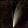 |
Fig. 1 Image of comet C/2020 F3 (NEOWISE) on 13.1 July 2020 UT, 8.6° field of view (celestial north to the top); 8 min exposure with 135 mm F/D = 2.5 telephoto lens from Indre-et-Loire (France). ©N. Biver. |
2 Observations of comet C/2020 F3 (NEOWISE)
2.1 IRAM30-m observations
In the frame of the IRAM director discretionary time proposal D01-20, 18 h of observing time with the IRAM 30-m radio telescope were allocated on 25–27 July 2020, between 15h and 21h local time (UT+2) to observe the exceptional comet C/2020 F3 (NEOWISE). Short additional observations were obtained pre-perihelion on 23.7 May 2020, under poor weather conditions at 3 and 2 mm wavelengths. As a typical summer weather pattern, afternoon cloudiness affected all the observations and the first 4–5 h were unstable and displayed relatively high atmospheric opacity (10–20 mm of precipitable water vapour – pwv). This affected the pointing and focusing accuracy of the telescope and resulted in a loss of beam efficiency. In July, the comet was also close to zenith during part of the observing runs, which had the advantage of limiting the impact of low atmospheric transmission. The last 1–2 h of each observing run in July generally yielded the best data quality and detections. The comet was tracked using orbital elements JPL#53 in May and JPL#14 in July and pointing errors were later estimated using JPL#15 orbital elements and the mapping of strong lines undertaken during the observations (see for example Fig. 3).
The IRAM 30-m observations used the EMIR (Carter et al. 2012), side band separation (2SB), dual polarisation, 3 mm, 2 mm, and 1 mm bands receiver, connected to the wide-band Fourier transform spectrometer (FTS, 4 × 8GHz, 195 kHz sampling) and VESPA high resolution autocorrelator (40–512 MHz bandwidth, 20–1250 kHz sampling). In order to cancel the sky emission, a wobbler switching mode at a frequency of 0.5 Hz was used, with reference sky positions at ±180″ in azimuth.
Table 1 summarises the setups used, integration time (including mapping), and amount of precipitable water vapour. Sample spectra are shown in Figs. 4–8 and the line-integrated intensity are provided in Tables 2–4. HCN, CH3OH, H2CO, CS, and H2S were clearly detected through at least two lines (Figs. 4-8), while the HNC and CH3CN (Fig. 5) lines are weaker. CO (Fig. 4) is only marginally detected. In Table 4, we provide the line intensity (or 3-σ upper limit) for molecules that were not detected and for which we averaged several lines. Although the comet activity was high, poor weather conditions did not help with regard to potential detections of more complex molecules that are sometimes observed in comets with lower activity levels (Biver et al. 2021).
2.2 Observations with NOEMA in single-dish mode
In parallel, the IRAM director also awarded discretionary time (proposal D20AC) for two tracks with the NOEMA interferometer, carried out on 22.3 July (2 mm band) and 7.8 August (1 mm band) under marginal summer weather as well. The interferometer was in its 10D compact configuration with ten antennas. The interferometric observations were interlaced with 2 min ON-OFF position-switch integrations every 25 min. The first run took place on 22 July from 5h30 to 11h UT tuned to 144.756 GHz in the lower sideband (LSB) and 160.244 GHz in the upper sideband (USB), both for the continuum (two ±2 × 3.872 GHz windows with a 2 MHz sampling per polarisation) and for line emissions in 25 windows of 62.5–312 MHz width with high spectral resolution (62.5 kHz), using the Poly-fix correlator. Beam efficiencies in single dish mode (ON–OFF or position-switched observations) of 0.78 (145 GHz) and 0.76 (160 GHz), estimated from planet observations, were used to convert the data in Tmb scale.
The second run on 7 August (16h20–20h20 UT) also suffered from poor weather conditions (pwv decreased from 10 to 4 mm at the end) and, also due to reduced cometary activity, yielded only marginal results. The receiver was tuned to 213.25 GHz (LSB) and 228.75 GHz (USB), and was connected to 20 windows with high spectral resolution (62.5 kHz) for the lines and two 7.774 GHz wide bands at 2 MHz spectral sampling for the continuum. Beam efficiencies values for the ON–OFF observations of 0.62 and 0.60, for 213 and 229 GHz respectively, were used. The continuum signal was marginally detected.
The two setups used are summarised in the last lines of Table 1 and sample spectra are shown in Figs. 9–12. The ON–OFF line-integrated intensity are provided in Table 5.
2.3 Observations with NOEMA in interferometric mode
While the interferometric data of 7 August 2020 could not be used due to bad atmospheric conditions, several lines were detected on 22 July 2020. The CS J(3–2) line near 147.0 GHz was detected with a signal to noise ratio of ~15 in line-integrated intensity. Seven CH3OH(J0 − J−1E) lines (J = 2, 3, 4, 5, 6, 7, 8) between 156.5 and 157.3 GHz were also detected with a lower signal to noise ratio (between 4.8 and 8.8). The measured fluxes integrated in the synthesised or primary beam are reported in Table 6, together with other line parameters (frequency, synthesised beam size, spectral integration range).
The line-integrated interferometric maps of the detected lines are presented in Fig. 13. The spectra extracted from the data cube at the position of the brightness peak on the line-integrated maps are presented in Fig. 14. Given the low signal-to-noise ratio of the spectra of the methanol lines, we present the average spectrum of the seven detected lines. The analysis of the continuum data is presented in Sect. 5. The offsets between the peak of the continuum and the CS and CH3OH were estimated to (∆α, ∆δ) = (−0.01, +0.08) ± 0.4″ and (0.00, +0.30) ± 0.34″, from the weighted average of the seven methanol lines, respectively. Thus, no significant offset between gas and the larger (mm size) dust is seen, suggesting their emission both peak at the nucleus position. The offsets (either tailward for the gas or sunward for the dust) observed by Faggi et al. (2021) on 9–20 July are not seen here. Faggi et al. (2021) observations may have been sensitive to smaller dust seen in the IR that was ejected with a larger velocity and in the sun-ward direction as was seen in the visible continuum images in early July.
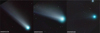 |
Fig. 2 Telescopic optical images of comet C/2020 F3 (NEOWISE) on 21.9, 26.9 July, and 6.9 August 2020 UT, close in time to the IRAM observations. North is to the top and the field-of-views (fov) are 40 × 40′. Corresponding estimates of Afρ (red band) were 10 000, 4300, and 1600 cm, respectively. The 20–40 s exposure at the focus of a 407 mm diameter telescope (F = 1750 mm) from Eure-et-Loire (France). ©N. Biver. |
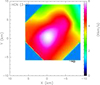 |
Fig. 3 Coarse map of the HCN(3–2) line-integrated intensity in the coma of comet C/2020 F3 (NEOWISE) on 27.7 July 2020 with the IRAM 30-m telescope. The intensity distribution is best matched assuming a distributed source with a scale length of 830 ± 360 km, but this corresponds to 1.6″, on the order of typical pointing instability especially in the afternoon. |
3 Data analysis
Several lines of HCN, CS, H2S, and CH3OH were detected with a signal-to-noise ratio (S/N) sufficient to derive precise information on the gas expansion velocity, outgassing pattern, and the temperature of the atmosphere of the comet.
3.1 Expansion velocity
The mean expansion velocity was determined from the shapes of the lines with highest S/N (Figs. 4–11). The mean values of the velocity in km s−1 at half the peak intensity on these lines (VHM, Biver et al. 2021) are (−1.07 ± 0.08;+1.16 ± 0.07), (−1.00 ± 0.02;+1.05 ± 0.03), and (−1.06 ± 0.18;+0.68 ± 0.04) for the 22, 26 July, and 7 August respectively. We adopted expansion velocities of 1.1, 1.0, and 0.85 km s−1, for these dates. The H2S lines (on 25–27 July, Fig. 4) suggest a lower velocity (−0.82 km s−1) than for all other molecules which is likely due to its shorter lifetime (τ(H2S) = 2000 s at rh = 0.71 au), combined with gas acceleration in the coma. Gas acceleration is also likely responsible for the increase in line width of the CS (J = 3–2) and CH3 OH lines between the line profiles seen in interferometric mode (6.3″ beam, Fig. 14) and single-dish (ON–OFF; 33″ beam, Fig. 9–11) mode. The inferred expansion velocity (means of the two VHM) are 0.91 km s−1 (CS (J = 3–2)) and 0.87 km s−1 (methanol average) from interferometric spectra and 1.20 ± 0.12 km s−1 (CS) and 1.37 ± 0.18 km s−1 (CH3OH) from the ON–OFF spectra. The S/N being too low on individual CH3OH spectra to estimate the line width with accuracy, we added the seven detected lines. To simulate acceleration in the coma as a function of the radial distance r (in km), we define vexp,var(r) as:
 (1)
(1)
which we use to fit the variation of observed line-widths, following Biver et al. (2011), with v0 = 0.6 km s−1 and xacc = 8.0.
We note that changing the expansion velocity from 1.0 to 0.85 km s−1 for H2S does not change the retrieved production rate, since most of the molecules are inside the beam and then  does not depend on the expansion velocity. For the other species, using velocity law (Eq. (1)), or the value that fits the observed line-width, does not significantly change the retrieved production rate either. The line shapes do not show significant asymmetry, which is not surprising since the phase angle was close to 90o – and a day versus night asymmetry in outgassing should be mostly seen in the plane of the sky, but it is not evident in the visible images at that time (Fig. 2).
3.2 Gas temperature
Rotational temperatures were measured for several series of methanol lines. Based on IRAM 30-m spectra, the measured values are: 73 ± 14, 64 ± 15, 69 ± 18, and 84 ± 9 K, respectively, for the 145–147, 165–169, 242, and 250–254 GHz series of methanol lines. The lines around 252 GHz are the best suited to probe the inner coma gas temperature (Tgas), while the rotational temperature of the lines around 145 and 242 GHz are expected to be lower than Tgas. As shown in Fig. 15, a model using Tgas = 90 K provides a good fit to the observed rotational temperatures. The modelled rotational temperatures are Trot(model, 145 GHz) = 62 K, Trot (model, 166 GHz) = 88 K, Trot(model, 242 GHz) = 73 K, and Trot(model, 252 GHz) = 81 K. For the May data, we used Tgas = 60 K, assuming a ~1/rh-dependence of the temperature (Biver et al. 2002).
NOEMA ON–OFF methanol data (also sampling a region that is twice larger due to a larger beam) of 22.4 July suggest a temperature of Tgas ~ 95 K (Fig. 16). If we exclude the J =15 and 16 lines below the 3-σ level, we have the retrieved Trot = 87 ± 19 K, while the lines at 145 GHz require a high value as well for Tgas: Trot (observed, 145 GHz) = 104 ± 17 K. The value of Tgas for the 7.8 August is not very well constrained: using the three detected methanol lines, we get  K. This suggests Tgas = 31–58 K, implying a very steep decrease with heliocentric distance (as
  ). We adopted a value of Tgas = 50 K for the 7.8 August observations.
The interferometric fluxes measured on the maps of seven methanol lines (J0–J−1E, with J = 2, 3, 4, 5, 6, 7, 8) were used to derive a rotational temperature in the inner coma. We find a value of Trot = 71 ± 11 K, which is marginally lower than the value at larger scales in the coma derived from ON–OFF data (87 ± 19 K). In order to simulate the observed increase of gas temperature in the coma we modelled Tgas with an increase from 50 to 125 K in the r = 100–100 000 km range following:
 (2)
(2)
The results of the comparison between observed versus simulated Trot values are provided in Table 7. The change of production rates derived from single dish data using Eq. (2) instead of T = 95 K is negligible for CS(3–2) and implies a reduction of less than 8% for CH3OH lines at 157 GHz.
Log of observations with IRAM telescopes.
3.3 Reference water production rate
The water production rate of comet C/2020 F3 was estimated from observations of the Lyman-α Hydrogen emission with the Solar Wind ANistropies (SWAN) instrument on the SOHO spacecraft from 51 days before to 66 days after perihelion (Combi et al. 2021). Unfortunately, there is a gap in the data at the time of IRAM observations, but the water production rate followed regularly the  molec. s−1 law during that period, implying
  molec. s−1 at the time of the July IRAM observations. For 23.7 May, the SWAN data gives
  molec. s−1. For 22.4 July and 7.8 August, the rounded values are:
  and 1 × 1029 molec. s−1, respectively.
The OH lines at 18 cm were detected on 24.7 July with the Green Bank Telescope (GBT) and on 24.6, 26.6, and 27.6 July with the Nançay radio telescope. The combination of GBT and Nançay data enabled a precise determination of the quenching of the OH maser and production rate, yielding a water production rate around 4.5 × 1029 molec. s−1 (Drozdovskaya et al., in prep.) on 24.7 July and around 4 × 1029 molec. s−1 for the 26–27 July period, value that we have adopted here. Table 8 summarises the parameters used to analyse the data and compute molecular abundances.
4 Production rates and abundances
4.1 Spatial distribution of CS from interferometric maps
There are several ways to study the distribution of molecules in the coma from radio interferometric data as obtained with ALMA or NOEMA. We may directly study the visibility distribution as a function of baseline length (as done for HCN, HNC, and H2CO in comets C/2012 F6 (Lemmon) and C/2012 S1 (ISON), Cordiner et al. 2014) or compare the ON–OFF and interferometric fluxes (as done for CS, SO, and CO in comet C/1995 O1 (Hale-Bopp), Boissier et al. 2007; Bockelée-Morvan et al. 2009). In the present case, the individual visibilities have too low S/N values and cannot be used. We thus study the single-dish (ON–OFF) to interferometric-flux ratio (R = FSD/FInt), which depends on the molecule distribution in the coma, as shaped by its release and dissociation processes between scales on the order of the Synthesized beam (~6″ or 3000 km) and of the antenna primary beam (that is 32.7″ or 16400 km). A distributed source in the coma will result in a higher ratio (R = FSD/FInt) than the value that would be expected for a pure nuclear production.
The study of the distribution of methanol commonly regarded as a pure parent species (direct release from the nucleus) is relatively straightforward, since it has a well known photo-dissociation rate. This is not the case for the CS radical which is produced by an unknown distributed source (recent measurement suggest that CS2 cannot be the only source of CS, Roth et al. 2021) and for which the photo-dissociation rate is also poorly known (Boissier et al. 2007; Biver et al. 2011).
We modelled the CS (J = 3−2) and CH3OH (J0−J−1 E, J = 2, 3, 4, 5, 6, 7, 8) ON–OFF and interferometric fluxes assuming different conditions in the coma: constant (95 K) or variable temperature (Eq. (2)) and constant (1.1 km s−1) or variable outflow velocity (Eq. (1)).
We report in Table 7 the CH3OH and CS ON–OFF to interferometric flux ratios ( and RCS) computed using the standard values for their radial extension: CH3OH released from the nucleus and the photo-dissociation rate of β0(CH3OH) = 1.31 × 10⁻⁵ s−1 (at 1au) as well as CS created by the photo-dissociation of CS2 (β0(CS2) = 1.7 × 10⁻³ s−1) and dissociated at a rate of β0(CS) = 2.5 × 10⁻⁵ s−1. These photo-dissociation rates can be converted into scale lengths in the coma of comet NEO-WISE at the time NOEMA observations. For the models with a constant velocity, we get: L(CS) = 16 642 km, L(CS2) = 245 km, and L(CH3OH) = 32 000 km. With models that include acceleration (Eq. (1)), we get: L(CS) = 18 300 km, L(CS2) = 125 km, and L(CH3OH) = 38 500 km. We note that the fact that the absolute flux scale calibration is performed in an independent way in interferometric and ON–OFF modes adds a 10% additional uncertainty on the flux ratio, taken into account in the error-bars σ(Robs). In Figs. 17 and 18, we plot
  for CS and CH3OH and various model parameter as a function of CS dissociation scale length (Fig. 17) or parent scale lengths (Fig. 18).
All ratios are lower than the observed values, suggesting that the gas distribution is more extended than expected. We note that the (T = 95 K, v = 1.1 km s–1) model is in 1-σ agreement with the observations but this temperature and velocity do not reproduce other observed characteristics (larger line widths and higher Trot in larger single-dish beams with respect to interferometric beams). This more extended distribution can be generated in two ways: (i) a slower dissociation (that is lower β and larger scale length in the coma) or (ii) a more distributed production (non-nuclear origin for CH3OH, larger scale length for the parent of CS).
The former is unlikely for CH3OH, since its photo-dissociation rate is well known and has been thoroughly used in the analysis of previous millimetre observations of comets without any indication that it might be incorrect. As mentioned above this is not the case for CS so we computed the ON–OFF-to-interferometric flux ratios (RCS) obtained assuming different values for β(CS). The results are presented in Fig. 17. In the models assuming constant outflow velocity, the observed and simulated flux ratios can be reconciled with CS scale length at least twice larger than the commonly used value. Assuming a variable temperature we have to go for extreme L(CS) values suggesting that the extended distribution we observe is due, rather, to a more extended production. The lower panel of Fig. 17 shows no solution assuming that the parent scale length of CS is that of the photo-dissociation of CS2.
To investigate the impact of a more distributed source on the distribution of CH3OH and CS, we computed ON–OFF to interferometric flux ratios using the standard β(CH3OH) and β(CS) and assuming different production scale lengths (LP) for both species. The results are presented in Fig. 18. Depending on the model, the production scale lengths which leads to the best fit results are in the range 200–2100 km for CH3OH and 700–3000 km for CS. Outgassing from icy grains could be responsible for a distributed source of most molecules in the first 1000–2000 km around the nucleus. We note that this is on the same order of magnitude as found for HCN from IRAM 30-m maps (LP = 470–1190 km, Fig. 3).
However Lp(CS) is always larger than Lp(CH3OH), with a difference on the order of 500 km (constant vexp) to 900 km (vexp, var), which is significantly larger than the ~200 km photo-dissociation scale length of CS2. This demonstrates again that CS2 cannot be the unique parent species for CS. With a lifetime τP = 450–1000 s at 0.615 au the unknown parent of CS would have a photo-dissociation rate β0,P in the range 4–48 × 10−4 s−1 at 1 au corresponding to a lifetime on the order of τP,0 = 2000 s at 1 au.
This is consistent with the results of Roth et al. (2021), deduced from ALMA compact array observations of comet C/2015 ER61 (PanSTARRS), and confirms that CS2 cannot be the only parent species for CS. We also use a parent lifetime of τP,0 = 3000 s, that is, about five times the CS2 lifetime to derive CS production rate from a still unknown other parent source. This values includes both the likely grain source and unknown parent contribution to the distribution of CS.
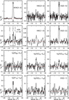 |
Fig. 4 Average spectra of HCN, HNC, CS, H2S H2CO, and CO detected in the coma of comet C/2020 F3 (NEOWISE) on 25–27 July 2020 with the IRAM 30-m telescope. The vertical scale is the main beam brightness temperature and the horizontal scale is the Doppler velocity in the comet rest frame, with respect to the strongest line. |
 |
Fig. 5 Spectrum of a series of CH3CN lines around 147 GHz on 25–27 July 2020 in the comet C/2020 F3 (NEOWISE) with IRAM 30-m. The vertical scale is the main beam brightness temperature and the horizontal scale is the Doppler velocity in the comet rest frame with respect to the (8,0)–(7,0) line. The frequency scale is also provided on the upper axis. |
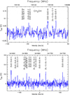 |
Fig. 6 Spectrum of a series of methanol lines around 145 GHz on 26–27 July and 242 GHz on 25.77 July 2020 in the comet C/2020 F3 (NEOWISE) with IRAM 30-m. The vertical scale is the main beam brightness temperature and the horizontal scale is the Doppler velocity in the comet rest frame with respect to the strongest line. The frequency scale is also provided on the upper axis. |
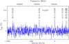 |
Fig. 7 Spectrum of a series of methanol lines around 165 GHz on 26.77 July 2020 in the comet C/2020 F3 (NEOWISE) with IRAM 30-m. The vertical scale is the main beam brightness temperature and the horizontal scale is the Doppler velocity in the comet rest frame with respect to the strongest line. The frequency scale is also provided on the upper axis. |
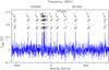 |
Fig. 8 Spectrum of a series of methanol lines around 252 GHz on 27.8 July 2020 in the comet C/2020 F3 (NEOWISE) with IRAM 30-m. The vertical scale is the main beam brightness temperature and the horizontal scale is the Doppler velocity in the comet rest frame with respect to the strongest line. The frequency scale is also provided on the upper axis. |
Line intensities from IRAM 30-m observations.
Line intensities from IRAM 30-m observations: 2–3 day averages.
Average line intensities from IRAM observations: searching for other species.
4.2 Production rates
Production rates were determined assuming a Haser density profile, with molecular lifetimes as provided in Biver et al. (2021). Collisional excitation with neutrals at Tgas and electrons and radiative processes (infrared or pumping via vibrational bands for HCN, HNC, CH3CN, H2CO, CH3OH, and CO) were taken into account. Daily and average production rates or upper limits are provided in Table 9. For non-detected species for which we could use several lines, we provide the 3-σ upper limit based on the weighted average of production rates derived from each individual line.
We used the constant velocity and temperature (no variation with distance to the nucleus) given in Table 8 to compute production rates of Table 9. If we use the expansion velocity and temperature profiles that varies with r for NOEMA data, this will decrease the CS and CH3OH production rates by ~7%. However, when taking into account also the production from a distributed source (Lp ~ 1500 km), then production rates are 12% higher, which is also the increase in HCN production rate based on IRAM 30-m map data with the best fit parent scale length of ~1000 km.
When taking into account the possible release of most molecules from a distributed source (e.g. icy grains) with the best temperature and velocity profile, all production rates and abundances relative to water (reference  is not sensitive to those scales) would generally be increased by about 10%. Nevertheless, the abundances relative to each other molecule observed at millimetre wavelengths would not be significantly affected. Since most observations were obtained under marginal observing conditions (the distributed source length LP = 1000–1500 km corresponding to 2–3″, which is a typical value for pointing rms), we prefer to remain cautious about the presence of a distributed source for all molecules.
For H2CO, we also computed the production rate assuming a parent scale length LP = 4200–8000 km, following the law LP ~ 2 × L(H2CO), where L(H2CO) is the formaldehyde photo-destruction scale length  . This is the maximum value suggested by Biver et al. (1999), which provides the best fit to the evolution of line intensity with offset position from the 25–27 July period. The reduced Chi-squares (modelled vs observed line intensities as a function of QP and LP(H2CO)) are
  , 1.5, and 1.1 for LP = 0, 1.5× and 2× L(H2CO), respectively.
The detection of the HNC lines (Fig. 4) with a small J3–2 to J1–0 intensity ratio of 6.9 ± 2.2 (compared to 17.6 for HCN lines) is consistent with the production of HNC in the coma. Assuming a parent scale length of Lp = 2000 km reduces the difference between QHNC based on the J=3–2 and the J = 1–0 lines, because the 1–0 line is observed with beam three times wider. An HNC distributed source with a parent scale length on the order of 1000-3000 km has been suggested by Cordiner et al. (2014, 2017) and Roth et al. (2021).
 |
Fig. 9 High resolution (62.5 kHz) spectra of CS, SO, H2CO, and CH3OH lines on 22.4 July 2020 in the coma of comet C/2020 F3 (NEOWISE) with the 10 NOEMA antennas in single dish mode. Scales are as in Fig. 4. |
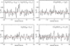 |
Fig. 10 Spectra of H2CO (sum of two lines), H2S, and CH3OH lines on 7.8 August 2020 in the coma of comet C/2020 F3 (NEOWISE) with the 10 NOEMA antennas in single dish mode. Spectral resolution has been degraded to 250 kHz due to limited signal-to-noise. Scales are as in Fig. 4. |
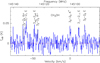 |
Fig. 11 Spectrum of a series of methanol lines around 145 GHz on 22.4 July 2020 in the comet C/2020 F3 (NEOWISE) with the 10 NOEMA antennas in single dish mode. The vertical scale is the main beam brightness temperature and the horizontal scale is the Doppler velocity in the comet rest frame with respect to the strongest line. The frequency scale is also provided on the upper axis. |
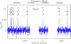 |
Fig. 12 Spectrum of a series of methanol lines around 157 GHz on 22.4 July 2020 in the comet C/2020 F3 (NEOWISE) with the ten NOEMA antennas in single dish mode. Scales are as in Fig. 11. |
4.3 Relative abundances
Abundances or 3-σ upper limits on the abundances relative to water, and lower limits on isotopic ratio, are provided in Table 10. Values measured in other comets are also provided for comparison: all abundances are within the range of values measured in comets.
Formally, HC3N is not detected, but the average of each of the NOEMA and IRAM observations in July yield a 2–3 σ signal suggesting an abundance relative to water on the order of 0.01%, consistent with values measured in other comets. The 3-σ upper limits given for five molecules (HNCO, NH2CHO, HCOOH, CH3CHO, and SO2) show that these molecules are not enriched in comet C/2020 F3 in comparison to other comets. Limits on isotopic ratios are provided for completeness, but are not significant.
The detection of an SO line (Fig. 9) on 22.4 July with NOEMA yields an abundance relative to water which is higher than observed in other comets and then the upper-limit derived from the IRAM 30-m observations. The line is present in both the low and high resolution spectrometer, although with a limited S/N. To explain the difference with the non-detection at IRAM 30-m 4 days later, SO needs to be produced by a more extended source than assumed (Lp ≫ 10 000 km) in order to be detected in the NOEMA 30″ beam but not in the IRAM 30-m 10″ beam, and exhibiting a strong dependence on the heliocentric distance. Another explanation could be related to the excitation of SO rotational levels: the NOEMA line is sampling a lower energy level (Eup = 29 K) than the transitions observed with IRAM 30-m (Eup = 44–57 K): any process leading to a much lower rotational temperature than modelled could partly explain the discrepancy. The simultaneous search for SO2 was attempted through several lines, but yielded upper limits in production that are not useful as they are twice higher than for SO.
The pre-perihelion observations in May are too marginal to be used in the study of heliocentric variation. However, the NOEMA single dish results provide useful complementary data to the IRAM 30-m observations for the evolution of the production rates with heliocentric distance (post-perihelion) which is plotted in Fig. 19. The fits to the heliocentric variations of production rates during the three weeks post-perihelion period are  , and
, and  , in units of 1026 molec. s−1.
Line intensities from observations with NOEMA in ON–OFF mode (10 antennas).
Line characteristics from observations with NOEMA in interferometric mode.
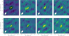 |
Fig. 13 Interferometric maps of the CS J = 3-2 and for each methanol J0 − J−1 E line (J = 2, 3, 4, 5, 6, 7, 8) as observed with NOEMA on 22 July 2020. The synthesised beam is shown on the bottom left corner. The maps were recentered on the brightness peak position (as found by fitting a point source to the visibility distribution). Contour intervals are 1 × σ, σ being the map rms (0.028 Jy km s−1 for CS J(3–2), and 0.036, 0.032, 0.038, 0.040, 0.032, 0.038, and 0.036 Jy km s−1 for the methanol J0 − J−1E lines, with J = 2, 3, 4, 5, 6, 7, and 8, respectively. |
 |
Fig. 14 Spectra extracted at the brightness peak position of the interferometric maps. The CS (J = 3–2) line is presented in the left panel while the sum of seven methanol lines (J0 – J−1E, J = 2, 3, 4, 5, 6, 7, 8) is displayed in the right panel. The vertical scale is the flux in Jy per beam and the horizontal scale is the Doppler velocity in the comet rest frame. |
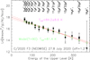 |
Fig. 15 Rotational diagram of the methanol lines around 252 GHz observed on 27.8 July 2020 (Fig. 8). The derived rotational temperature (84 ± 9 K) is close to the expected value for a gas temperature of 90 K in the coma of comet C/2020 F3 (NEOWISE; model in green). |
5 Analysis of the continuum radiation
The interferometric maps of the continuum radiation measured at 144.8 GHz (LSB) and 160.2 GHz (USB) frequencies on 22 July 2020 are presented in Fig. 20. The detected emission is due to the thermal emission of dust particles in the coma. Indeed, the decrease of the visibilities with increasing baseline length B1 (Fig. 20) is characteristics of the brightness distribution expected for a steady-state dust coma with a local density ∝ 1/r2, where r is the cometocentric distance. Here, we recall that foran unresolved source, visibilities display a constant value independent of B1. We also show in Fig. 20 (central plots) the total flux measured within circular apertures as a function of the aperture radius, ρ. The nearly linear trend for ρ <8″ is a clear evidence for dust-coma emission. The plateau observed for ρ >8″ is due to large-scale spatial filtering set by the shortest baseline lengths and is in agreement with the estimated largest recoverable scale of ~10″.
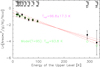 |
Fig. 16 Rotational diagram of the methanol lines around 157 GHz observed on 22.4 July 2020 (Fig. 12). The derived rotational temperature (97 ± 17 K) is close to the expected value for a gas temperature of 95 K in the coma of comet C/2020 F3 (NEOWISE; model in green). |
5.1 Upper limit on nucleus size
A strict conservative upper limit on the nucleus flux density can be obtained by selecting the data recorded by the longest baselines (i.e. sensitive to the smaller scales). Using baseline lengths Bl > 22kλ and applying a point-source fit to the visibilities, the inferred flux densities are 0.7 ± 0.4 mJy and 1.7 ± 0.2 mJy, at LSB and USB frequencies, respectively; thus, this gives us an average of 1.2 ± 0.2 mJy for the median frequency of 152.5 GHz.
We also performed a two-parameter fit to the measured visibilities using a linear combination of a dust-coma visibility profile and a constant (point-source) profile. The inferred point-source fluxes are 0.5 ± 0.8 mJy (LSB) and 0.4 ± 0.3 mJy (USB), showing that there is no hint of nucleus detection in the data. The most stringent upper limit is for USB data, i.e., 0.9 mJy (3-σ) at 160.244 GHz, which we used to determine an upper limit on the nucleus size.
Our size determination is based on the Near-Earth Asteroid Thermal Model (NEATM, Harris 1998). We assumed a beaming factor n = 0.7 and a bolometric emissivity of 0.8, consistent with the analysis of 8P/Tuttle interferometric data made by Boissier et al. (2011). The derived 3-σ upper limit for the nucleus radius of C/2020 F3 (NEOWISE) is r < 4.72 km. This upper limit is about twice the value (≈2.5 km) derived by Bauer et al. (2020) from the WISE infrared data. With r = 2.5 km we would have expected a 0.25 mJy signal from the nucleus, below our point-source sensitivity after removing the dust contribution.
5.2 Dust mass loss rate
The dust mass loss rate was computed using the dust thermal model of Bockelée-Morvan et al. (2017). This model computes the wavelength-dependent absorption coefficient Qabs and temperature of dust particles as a function of grain size using the Mie theory combined with an effective medium theory in order to consider mixtures of different materials. Effective medium theories (EMT) allow us to calculate an effective refractive index for a medium made of a matrix with inclusions of another material. The Maxwell–Garnett mixing rule is used in this model, and is also applied to consider the porosity of the grains, set to be 50% at maximum (Bockelée-Morvan et al. 2017). The thermal spectrum is computed by summing the contributions of the individual dust particles which are within the field of view. The size distribution of the dust particles is described by a power-law n(a) ∝ a−β, where β is the size index and the particle radius takes values from amin to amax. The dust density is taken equal to ρdust = 800 kg m−3, which corresponds to the mean value of comet 67P dust particles (Fulle et al. 2018). The local density of the dust particles in the coma is described by the Haser model and follows a 1/(r2 vdust(a)) variation. vdust(a) is the expansion velocity of particles of size a, and is assumed to vary ∝ a−0.5 as expected for gas drag. The total dust production rate, summing all sizes with their respective mass contribution, is given by Qdust.
The literal expression of the flux density is:
 (3)
(3)
with the total dust production rate given by:
 (4)
(4)
In Eq. (3), Bv(Tdust(a)) is the black-body radiation at the temperature, Tdust(a). The integrals are over the field of view (fov of radius ρFOV and volume integral on the line of sight (z = −∞ to +∞) within θ < 2π, as well as the projected radius ρ < ρFOV) and size range.
We consider that the dust particles are made of amorphous carbon with inclusions of amorphous olivine with a Fe:Mg composition of 50:50 (see Bockelée-Morvan et al. 2017, for the references for optical constants). The mass ratio between carbon and olivine is 1. The maximum liftable size from the surface of C/2020 F3’s nucleus on 22 July 2020 is estimated to be amax = 0.7 m, based on a H2O production rate of 6 × 1029 s−1, and assuming a nucleus density of 500 kg m−3 and a nucleus radius of 2.5 km (V. Zakharov, priv. comm., see Zakharov et al. 2018, 2021). The minimum particle size is set to amin = 0.5 µm, but model results are not sensitive to this parameter, since the thermal emission in the millimetre domain is more efficient for large particles. The terminal velocity of the dust particles is determined following Crifo & Rodionov (1997), using the nucleus and dust gas parameters described above, and a gas expansion velocity of 1.1 km s−1: the value inferred for 10-µm particles is 260 ms−1.
We present in Table 11 the dust production rate inferred for size distribution indexes β of 2.5, 3.0, and 3.5. These values are in the range of 6–18 × 103 kg s−1. We used the total flux densities measured on the interferometric maps within an aperture radius ρ = 5″. The production rates determined for the USB and LSB data are consistent within the uncertainties. The USB and LSB frequencies are too close to derive a spectral index that could constrain the size index. As a matter of fact, the derived spectral index (defined as Fν ∝ να) is α = 1.2 ± 1.6. Spectral indexes derived from the model outputs range from 2.0 and 2.12.
The derived dust production rate is not so sensitive to the assumed dust composition, since large particles (with size parameter x = 2πα/λ ≫ 1, and Qabs ~ 1) are the most efficient emitters in the mm domain. On the other hand, this strongly relies on the assumed dust size distribution index (Table 11), maximum particle size, amax, and dust particles volumetric density. For example, increasing the maximum particle size by a factor 2 (i.e., amax = 1.4 m), the inferred Qdust values are 30–40% higher.
The derived dust-to-gas ratio  in mass for C/2020 F3 on 22 July is between 0.37 to 0.94. This range overlaps with the range of values (0.7–2.4) determined for 67P/Churyumov-Gerasimenko from the total water loss rate and the total mass loss of the nucleus over the whole Rosetta mission (Pätzold et al. 2019; Choukroun et al. 2020).
In previous studies of the dust thermal radio continuum from comets, the velocity of the dust particles contributing to the emission is assumed to not vary with particle size. The dust mass within the field of view is directly derived from the measured flux density using assumptions or calculations of the so-called dust opacity (e.g. Jewitt & Luu 1990; Altenhoff et al. 1999; Boissier et al. 2012). The dust opacities at 145 GHz derived from our thermal model for amax = 0.7m are 4.5 × 10⁻³, 1.2 × 10⁻², and 7.3 × 10⁻² kg m−2, for β = 2.5, 3, and 3.5, respectively.
Observed and simulated rotational temperatures of CH3OH and integrated fluxes ratios with NOEMA.
Adopted model parameters.
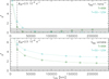 |
Fig. 17 Relative deviation between simulated and observed ON–OFF-to-interferometric flux ratio, |

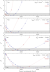 |
Fig. 18 Relative deviation between observed and simulated ON–OFF-to-interferometric flux ratio (R), |

Production rates.
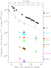 |
Fig. 19 Production rates of comet C/2020 F3 (NEOWISE) post-perihelion (13 July to 14 August 2020). The H2O data points are from Combi et al. (2021) and (Drozdovskaya et al., in prep.). The Afρ values have been estimated from digital (red layer) images, as in Fig. 2, and corrected for the phase angle (Schleicher 2007; Markus 2007). |
6 Discussion and conclusion
We determined production rates and molecular abundances for comet C/2020 F3 (NEOWISE) with a good level of accuracy despite adverse observing conditions. Eight molecules, namely, HCN, HNC, CH3CN, H2S, CS, CH3OH, H2CO, and CO, were detected and good upper limits on the abundances of six other species have been determined. All abundances are within the range of values observed in other comets.
The heliocentric variation of the CH3OH, CS, and CH3CN production rate is not as steep as that of water. The marginal detection of a single line at 0.97 AU of H2S, needs to be taken with caution to draw any definitive conclusion on the evolution of the H2S production rate over time. Nevertheless, these species are more volatile than water which could explain a shallower decrease of their production when the comet receded from the sun. On the other hand, the H2CO production rate, or its parent production rate varies steeply with heliocentric distance (Fig. 19). Such a trend is seen for larger distances from the Sun in the case of comet Hale-Bopp (Biver et al. 2002). Fray et al. (2006) interpreted this trend as H2CO coming from the thermal degradation of a parent such as a polymer like POM in the dust grains. This production process of H2CO is then dependent on dust production and temperature which varies steeply with heliocentric distance. Since the dust production in comet C/2020 F3 also varied steeply with heliocentric distance ( , Fig. 19), a similar explanation could be invoked.
CO was marginally detected and we inferred a relatively low abundance (3.2%) for this comet. This low abundance could explain the steep variation of the visual activity of the comet with heliocentric distance and lack of strong activity beyond ~1.6 au from the Sun4 that is responsible for its late discovery.
A lack of abundant hyper-volatiles like CO in this comet could explain the absence of sustained activity beyond some distance from the Sun. A similar behaviour was observed for the short period comet 67P (Biver et al. 2019; Läuter et al. 2020) which is similarly CO-poor.
Faggi et al. (2021) observed comet C/2020 F3 (NEOWISE) in the infrared at similar epochs. Between 20 July and 08 August 2020 they found similar production rates and abundances for CH3OH and CO. The trend of having CH3OH/H2O decreasing towards shorter heliocentric distance is also observed in the IR. The comparison for H2CO is not straightforward as we assume and generally find that most of H2 CO is coming from a large distributed source (Lp = 4200–8000 km) that infrared small aperture spectroscopy would not see. Nevertheless, when assuming that H2CO would come solely from the nucleus, we find an abundance relative to water (0.3%) similar to that measured in the IR. The HCN abundance relative to water measured in the IR (Faggi et al. 2021) is twice higher than inferred from the radio. Such a trend has been observed in many other comets and still needs to be resolved.
The interferometric continuum maps obtained on 22.4 July, yielded an upper limit on the nucleus diameter of 9.4 km, which is twice the value inferred by Bauer et al. (2020) from the infrared NEOWISE data. The dust production rate derived from the dust continuum emission, leads to a mass dust-to-gas ratio  between 0.4 and 0.9, encompassing the mean values for 67P (0.85 for dust-to-water, 0.64 for dust-to-volatile ratios, Choukroun et al. 2020). The dust-to-gas ratio in comets is often poorly constrained (0.1–10, e.g. Boissier et al. 2014; Choukroun et al. 2020) especially due to uncertainty on the mass distribution index β, maximum dust size, and without constraints on the spectral index from observations on a wide range of wavelengths. The dust-to-gas ratio of C/2020 F3 is relatively low, but it may also have varied over time: the
  was at its lowest (Fig. 19) at the time of NOEMA observations.
In summary, comet NEOWISE exhibited a high level of activity around perihelion with typical molecular abundances, on the high side for H2S, and low side for CO and the dust-to-gas ratio. We found that CS is produced by an unknown parent with a lifetime of ~2000 s at 1 au. Our observations focused on the 3–5 weeks period post-perihelion and suggested that the H2CO abundance decreased with heliocentric distance likely following the dust-to-gas ratio evolution.
Molecular abundances in comet C/2020 F3.
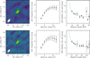 |
Fig. 20 2 mm continuum emission of comet C/2020 F3 (NEOWISE) obtained on 22 July 2020 UT with NOEMA. Top and bottom panels refer to LSB (144.8 GHz) and USB (160.2 GHz) data, respectively. Left: interferometric maps with the synthesised interferometric beam (8.5 × 4.6″ in LSB and 8.0 × 4.1″ in USB) plotted in the bottom left corner. Contour intervals are 2 × σ, σ being the map rms noise (with σ = 0.19 and 0.28 mJy beam−1 in LSB and USB, respectively). Centre: total flux as a function of aperture radius. Right: real part of the visibilities as a function of baseline length expressed in units of kλ where λ is the wavelength (dots with errors); the curve shows the expected visibilities for an isotropic dust coma with a local density ∝ 1/r2, where r is the cometocentric distance. |
Dust continuum and production rates.
Acknowledgements
This work is based on observations carried out under projects number D01-20 and 114-19 with the IRAM 30-m telescope and D20AC with NOEMA. IRAM is supported by the Institut Nationnal des Sciences de l’Univers (INSU) of the French Centre national de la recherche scientifique (CNRS), the Max-Planck-Gesellschaft (MPG, Germany), and the Spanish IGN (Instituto Geográfico Nacional). We gratefully acknowledge the support from the IRAM staff for its support during the observations. The data were reduced and analysed thanks to the use of the GILDAS, class software (http://www.iram.fr/IRAMFR/GILDAS). This research has been supported by the Programme national de planétologie of INSU. N.X.R. acknowledges support by the NASA Postdoctoral Program at the NASA Goddard Space Flight Center, administered by Universities Space Research Association under contract with NASA. Additional support from the NSF grant AST-2009253 for M.A.C., and by the Planetary Science Division Internal Scientist Funding Program through the Fundamental Laboratory Research (FLaRe) work package (M.A.C. & N.X.R.).
References
- Altenhoff, W. J., Bieging, J. H., Butler, B., et al. 1999, A&A, 348, 1020 [NASA ADS] [Google Scholar]
- Altwegg, K., & Bockelée-Morvan, D. 2003, Space Sci. Rev., 106, 139 [Google Scholar]
- Bauer, J. M., Mainzer, A., Gicquel, A., et al. 2020, AAS Meeting, 52, 316.04 [Google Scholar]
- Biver, N., Bockelée-Morvan, D., Crovisier, J., et al. 1999, AJ, 118, 1850 [NASA ADS] [CrossRef] [Google Scholar]
- Biver, N., Bockelée-Morvan, D., Crovisier, J., et al. 2002, Earth Moon Planets, 90, 323 [Google Scholar]
- Biver, N., Bockelée-Morvan, D., Colom, P., et al. 2011, A&A, 528, A142 [NASA ADS] [CrossRef] [EDP Sciences] [Google Scholar]
- Biver, N., Bockelée-Morvan, D., Hofstadter, M., et al. 2019, A&A, 630, A19 [NASA ADS] [CrossRef] [EDP Sciences] [Google Scholar]
- Biver, N., Bockelée-Morvan, D., Boissier, J., et al. 2021, A&A, 648, A49 [EDP Sciences] [Google Scholar]
- Bockelée-Morvan, D., & Biver, N. 2017, Philos. Trans. Roy. Soc. A, 375, 20160252 [CrossRef] [Google Scholar]
- Bockelée-Morvan, D., Henry, F., Biver, N., et al. 2009, A&A, 505, 825 [NASA ADS] [CrossRef] [EDP Sciences] [Google Scholar]
- Bockelée-Morvan, D., Calmonte, U., Charnley, S., et al. 2015, Space Sci. Rev., 197, 47 [Google Scholar]
- Bockelée-Morvan, D., Rinaldi, G., Erard, S., et al. 2017, MNRAS, 469, S443 [CrossRef] [Google Scholar]
- Boissier, J., Bockelé-Morvan, D., Biver, N. 2007, A&A, 475, 1131 [NASA ADS] [CrossRef] [EDP Sciences] [Google Scholar]
- Boissier, J., Groussin, O., Jorda, L., et al. 2011, A&A, 528, A54 [NASA ADS] [CrossRef] [EDP Sciences] [Google Scholar]
- Boissier, J., Bockelée-Morvan, D., Biver, N., et al. 2012, A&A, 542, A73 [NASA ADS] [CrossRef] [EDP Sciences] [Google Scholar]
- Boissier, J., Bockelée-Morvan, D., Biver, N., et al. 2014, Icarus, 228, 197 [NASA ADS] [CrossRef] [Google Scholar]
- Brasser, R., & Morbidelli, A. 2013, Icarus, 225, 40 [Google Scholar]
- Carter, M., Lazareff, B., Maier, D. et al. 2012, A&A, 538, A89 [NASA ADS] [CrossRef] [EDP Sciences] [Google Scholar]
- Choukroun, M., Altwegg, K., Kührt, E., et al. 2020, Space Sci. Rev., 216, 44 [CrossRef] [Google Scholar]
- Colom, P., Gérard, E., Crovisier, J., et al. 1997, Earth Moon Planets, 78, 37 [NASA ADS] [CrossRef] [Google Scholar]
- Combi, M. R., Mäkinen, T. T., Bertaux, J.-L., Quémerais, E. & Ferron, S. 2021, ApJ, 907, L38 [NASA ADS] [CrossRef] [Google Scholar]
- Cordiner, M. A., Remijan, A. J., Boissier, J., et al. 2014, ApJ, 792, 2 [Google Scholar]
- Cordiner, M. A., Boissier, J., Charnley, S. B., et al. 2017, ApJ, 838, 147 [Google Scholar]
- Crifo, J. F., & Rodionov, A. V. 1997, Icarus, 127, 319 [NASA ADS] [CrossRef] [Google Scholar]
- Drahus, M., Guzik, P., Stephens, A. et al. 2020, Astron. Tel. #13945 [Google Scholar]
- Faggi, S., Lippi, M., Camarca, M., et al. 2021, AJ, 162, 178 [NASA ADS] [CrossRef] [Google Scholar]
- Fray, N., Bénilan, Y., Biver, N. et al. 2006, Icarus, 184, 239 [NASA ADS] [CrossRef] [Google Scholar]
- Fulle, M., Bertini, I., Della Corte, V., et al. 2018, MNRAS, 476, 2835 [NASA ADS] [CrossRef] [Google Scholar]
- Harris, A. W. 1998, Icarus, 131, 291 [Google Scholar]
- Hartogh, P., Lis, D. C., Bockelée-Morvan, D., et al. 2011, Nature, 478, 218 [Google Scholar]
- Jewitt, D., & Luu, J. 1990, ApJ, 365, 738 [NASA ADS] [CrossRef] [Google Scholar]
- Läuter, M., Kramer, T., Rubin, M. & Altwegg, K. 2020, MNRAS, 498, 3995 [CrossRef] [Google Scholar]
- Masiero, J. 2020, CBET, 4740 [Google Scholar]
- Markus, J. N. 2007, Int. Comet Q., 29, 39 [NASA ADS] [Google Scholar]
- Müller, H. S. P., Schlöder, F., Stutzki, J., & Winnewisser, G. 2005, J. Mol. Struct., 742, 215 [Google Scholar]
- O’Brien, D.P., Walsh, K.J., Morbidelli, A., Raymond, S.N., & Mandell, A.M. 2014, Icarus, 239, 74 [CrossRef] [Google Scholar]
- Pätzold, M., Andert, T. P., Hahn, M., et al. 2019, MNRAS, 483, 2337 [CrossRef] [Google Scholar]
- Pickett, H. M., Poynter, R. L., Cohen, E. A., et al. 1998, J. Quant. Spec. Radiat. Transf., 60, 883 [Google Scholar]
- Roth, N. X., Milam, S. N., Cordiner, M. A., et al. 2021, ApJ, 921, 14 [NASA ADS] [CrossRef] [Google Scholar]
- Schleicher, D. G. 2007, Icarus, 191, 322 [NASA ADS] [CrossRef] [Google Scholar]
- Zakharov, V. V., Ivanovski, S. L., Crifo, J.-F., et al. 2018, Icarus, 312, 121 [NASA ADS] [CrossRef] [Google Scholar]
- Zakharov, V. V., Rodionov, A. V., Fulle, M., et al. 2021, Icarus, 354, 114091 [NASA ADS] [CrossRef] [Google Scholar]
Nakano Note 4202, http://www.oaa.gr.jp/~oaacs/nk/nk4202.htm
All Tables
Observed and simulated rotational temperatures of CH3OH and integrated fluxes ratios with NOEMA.
All Figures
|
Fig. 1 Image of comet C/2020 F3 (NEOWISE) on 13.1 July 2020 UT, 8.6° field of view (celestial north to the top); 8 min exposure with 135 mm F/D = 2.5 telephoto lens from Indre-et-Loire (France). ©N. Biver. |
| In the text | |
|
Fig. 2 Telescopic optical images of comet C/2020 F3 (NEOWISE) on 21.9, 26.9 July, and 6.9 August 2020 UT, close in time to the IRAM observations. North is to the top and the field-of-views (fov) are 40 × 40′. Corresponding estimates of Afρ (red band) were 10 000, 4300, and 1600 cm, respectively. The 20–40 s exposure at the focus of a 407 mm diameter telescope (F = 1750 mm) from Eure-et-Loire (France). ©N. Biver. |
| In the text | |
|
Fig. 3 Coarse map of the HCN(3–2) line-integrated intensity in the coma of comet C/2020 F3 (NEOWISE) on 27.7 July 2020 with the IRAM 30-m telescope. The intensity distribution is best matched assuming a distributed source with a scale length of 830 ± 360 km, but this corresponds to 1.6″, on the order of typical pointing instability especially in the afternoon. |
| In the text | |
|
Fig. 4 Average spectra of HCN, HNC, CS, H2S H2CO, and CO detected in the coma of comet C/2020 F3 (NEOWISE) on 25–27 July 2020 with the IRAM 30-m telescope. The vertical scale is the main beam brightness temperature and the horizontal scale is the Doppler velocity in the comet rest frame, with respect to the strongest line. |
| In the text | |
|
Fig. 5 Spectrum of a series of CH3CN lines around 147 GHz on 25–27 July 2020 in the comet C/2020 F3 (NEOWISE) with IRAM 30-m. The vertical scale is the main beam brightness temperature and the horizontal scale is the Doppler velocity in the comet rest frame with respect to the (8,0)–(7,0) line. The frequency scale is also provided on the upper axis. |
| In the text | |
|
Fig. 6 Spectrum of a series of methanol lines around 145 GHz on 26–27 July and 242 GHz on 25.77 July 2020 in the comet C/2020 F3 (NEOWISE) with IRAM 30-m. The vertical scale is the main beam brightness temperature and the horizontal scale is the Doppler velocity in the comet rest frame with respect to the strongest line. The frequency scale is also provided on the upper axis. |
| In the text | |
|
Fig. 7 Spectrum of a series of methanol lines around 165 GHz on 26.77 July 2020 in the comet C/2020 F3 (NEOWISE) with IRAM 30-m. The vertical scale is the main beam brightness temperature and the horizontal scale is the Doppler velocity in the comet rest frame with respect to the strongest line. The frequency scale is also provided on the upper axis. |
| In the text | |
|
Fig. 8 Spectrum of a series of methanol lines around 252 GHz on 27.8 July 2020 in the comet C/2020 F3 (NEOWISE) with IRAM 30-m. The vertical scale is the main beam brightness temperature and the horizontal scale is the Doppler velocity in the comet rest frame with respect to the strongest line. The frequency scale is also provided on the upper axis. |
| In the text | |
|
Fig. 9 High resolution (62.5 kHz) spectra of CS, SO, H2CO, and CH3OH lines on 22.4 July 2020 in the coma of comet C/2020 F3 (NEOWISE) with the 10 NOEMA antennas in single dish mode. Scales are as in Fig. 4. |
| In the text | |
|
Fig. 10 Spectra of H2CO (sum of two lines), H2S, and CH3OH lines on 7.8 August 2020 in the coma of comet C/2020 F3 (NEOWISE) with the 10 NOEMA antennas in single dish mode. Spectral resolution has been degraded to 250 kHz due to limited signal-to-noise. Scales are as in Fig. 4. |
| In the text | |
|
Fig. 11 Spectrum of a series of methanol lines around 145 GHz on 22.4 July 2020 in the comet C/2020 F3 (NEOWISE) with the 10 NOEMA antennas in single dish mode. The vertical scale is the main beam brightness temperature and the horizontal scale is the Doppler velocity in the comet rest frame with respect to the strongest line. The frequency scale is also provided on the upper axis. |
| In the text | |
|
Fig. 12 Spectrum of a series of methanol lines around 157 GHz on 22.4 July 2020 in the comet C/2020 F3 (NEOWISE) with the ten NOEMA antennas in single dish mode. Scales are as in Fig. 11. |
| In the text | |
|
Fig. 13 Interferometric maps of the CS J = 3-2 and for each methanol J0 − J−1 E line (J = 2, 3, 4, 5, 6, 7, 8) as observed with NOEMA on 22 July 2020. The synthesised beam is shown on the bottom left corner. The maps were recentered on the brightness peak position (as found by fitting a point source to the visibility distribution). Contour intervals are 1 × σ, σ being the map rms (0.028 Jy km s−1 for CS J(3–2), and 0.036, 0.032, 0.038, 0.040, 0.032, 0.038, and 0.036 Jy km s−1 for the methanol J0 − J−1E lines, with J = 2, 3, 4, 5, 6, 7, and 8, respectively. |
| In the text | |
|
Fig. 14 Spectra extracted at the brightness peak position of the interferometric maps. The CS (J = 3–2) line is presented in the left panel while the sum of seven methanol lines (J0 – J−1E, J = 2, 3, 4, 5, 6, 7, 8) is displayed in the right panel. The vertical scale is the flux in Jy per beam and the horizontal scale is the Doppler velocity in the comet rest frame. |
| In the text | |
|
Fig. 15 Rotational diagram of the methanol lines around 252 GHz observed on 27.8 July 2020 (Fig. 8). The derived rotational temperature (84 ± 9 K) is close to the expected value for a gas temperature of 90 K in the coma of comet C/2020 F3 (NEOWISE; model in green). |
| In the text | |
|
Fig. 16 Rotational diagram of the methanol lines around 157 GHz observed on 22.4 July 2020 (Fig. 12). The derived rotational temperature (97 ± 17 K) is close to the expected value for a gas temperature of 95 K in the coma of comet C/2020 F3 (NEOWISE; model in green). |
| In the text | |
|
Fig. 17 Relative deviation between simulated and observed ON–OFF-to-interferometric flux ratio, |
| In the text | |
|
Fig. 18 Relative deviation between observed and simulated ON–OFF-to-interferometric flux ratio (R), |
| In the text | |
|
Fig. 19 Production rates of comet C/2020 F3 (NEOWISE) post-perihelion (13 July to 14 August 2020). The H2O data points are from Combi et al. (2021) and (Drozdovskaya et al., in prep.). The Afρ values have been estimated from digital (red layer) images, as in Fig. 2, and corrected for the phase angle (Schleicher 2007; Markus 2007). |
| In the text | |
|
Fig. 20 2 mm continuum emission of comet C/2020 F3 (NEOWISE) obtained on 22 July 2020 UT with NOEMA. Top and bottom panels refer to LSB (144.8 GHz) and USB (160.2 GHz) data, respectively. Left: interferometric maps with the synthesised interferometric beam (8.5 × 4.6″ in LSB and 8.0 × 4.1″ in USB) plotted in the bottom left corner. Contour intervals are 2 × σ, σ being the map rms noise (with σ = 0.19 and 0.28 mJy beam−1 in LSB and USB, respectively). Centre: total flux as a function of aperture radius. Right: real part of the visibilities as a function of baseline length expressed in units of kλ where λ is the wavelength (dots with errors); the curve shows the expected visibilities for an isotropic dust coma with a local density ∝ 1/r2, where r is the cometocentric distance. |
| In the text | |
Current usage metrics show cumulative count of Article Views (full-text article views including HTML views, PDF and ePub downloads, according to the available data) and Abstracts Views on Vision4Press platform.
Data correspond to usage on the plateform after 2015. The current usage metrics is available 48-96 hours after online publication and is updated daily on week days.
Initial download of the metrics may take a while.